RIS-Assisted Sensing: A Nested Tensor Decomposition-Based Approach

Abstract

We study a monostatic multiple-input multiple-output sensing scenario assisted by a reconfigurable intelligent surface using tensor signal modeling. We propose a method that exploits the intrinsic multidimensional structure of the received echo signal, allowing us to recast the target sensing problem as a nested tensor-based decomposition problem to jointly estimate the delay, Doppler, and angular information of the target. We derive a two-stage approach based on the alternating least squares algorithm followed by the estimation of the signal parameters via rotational invariance techniques to extract the target parameters. Simulation results show that the proposed tensor-based algorithm yields accurate estimates of the sensing parameters with low complexity.

I Introduction

Reconfigurable intelligent surfaces (RISs) have grown rapidly as a transformative technology and one of the most promising advancements for the next generation of wireless communication systems. RISs are important for mitigating coverage holes in wireless networks and overcoming blockages, especially for higher frequency bands [1]. RISs also have the potential to improve sensing/tracking tasks performed by the base station (BS) that do not fall under the conventional communications-only umbrella of the BS. Therefore, RISs have the potential to be an integral component in supporting integrated sensing and communications (ISAC) technology [2].

In [3], the authors considered an RIS to improve target detection in multiple-input multiple-output (MIMO) radar systems by properly adjusting the RIS phase shifts and the radar waveform. The authors in [4] deal with how to deploy an RIS to improve the spatial diversity of a radar system by creating an additional virtual line-of-sight (LOS) path between the radar and the desired target. The authors in [5] investigate an RIS-assisted non-line-of-sight (NLOS) sensing scenario and propose both an active and passive beamforming design that minimizes the Cramér–Rao lower bound. The work in [6] proposes a scenario with a target-mounted RIS that aims to enhance the sensing performance for the desired targets while preventing the detection of the target by eavesdroppers. Finally, [7] proposes a parameter estimation method for an RIS-assisted monostatic scenario in which a generalized likelihood ratio test is designed. The approach involves a four-dimensional search over the delay-Doppler-azimuth-elevation parameters that uses a repetitive RIS phase-shift profile to decompose the four-dimensional search into separate delay-Doppler and azimuth-elevation search problems.

Our previous work in [8] addresses the problem of parameter estimation for a single-input single-output (SISO) sensing system by exploiting the intrinsic multidimensional structure of the received echo signal at the BS. In this paper, we generalize the idea to the MIMO case. To cope with this more challenging scenario, we propose a nested tensor decomposition based sensing (NTBS) algorithm for RIS-assisted monostatic sensing [9]. Our algorithm estimates the desired parameters by exploiting the inherent geometrical structure of the problem and recasting the received echo signal as a fourth-order nested tensor model. The NTBS method is a two-stage algorithm based on alternating least squares (ALS), which initially solves the parameter estimation problem iteratively and, in the final step, employs the well-known estimation of the signal parameters via rotational invariance techniques (ESPRIT) algorithm [10, 11] to extract the delay, Doppler, and angle estimates. Our simulation results show the impact of the system parameters on estimation performance, as well as computational complexity.

Notation: Scalars, vectors, matrices, and tensors are respectively represented as $a,\boldsymbol{a},\boldsymbol{A}$, and $\boldsymbol{\mathcal{A}}$. Also, $\boldsymbol{A}^{*}$, $\boldsymbol{A}^{\text{T}}$, $\boldsymbol{A}^{\text{H}}$, and $\boldsymbol{A}^{\dagger}$ respectively stand for the conjugate, transpose, Hermitian transpose, and pseudoinverse of a matrix $\boldsymbol{A}$. The $j$th column of $\boldsymbol{A}\in\mathbb{C}^{I\times J}$ is denoted by $\boldsymbol{a}_{j}\in\mathbb{C}^{I\times 1}$. The operator D$(\cdot)$ converts a vector into a diagonal matrix, $\text{D}_{j}(\boldsymbol{B})$ forms a diagonal matrix $R\times R$ out of the $j$th row of $\boldsymbol{B}\in\mathbb{C}^{J\times R}$. The matrix $\boldsymbol{I}_{N}$ denotes an identity matrix of size $N\times N$. The $n$th mode product between a tensor and a matrix is given by $\boldsymbol{\mathcal{A}}\times_{n}\boldsymbol{B}=\boldsymbol{B}\left[\boldsymbol{\mathcal{A}}\right]_{(n)}$. The symbols $\otimes$, $\diamond$, and $\odot$ indicate the Kronecker, Khatri-Rao, and Hadamard products, respectively. Element-wise division is indicated by $\oslash$.

II System Model

Figure 1: RIS-assisted MIMO Monostatic Sensing

Figure 2: Time-domain protocol of the proposed RIS design.

Consider a downlink monostatic RIS scenario, as shown in Figure 1. The BS has multiple antennas and is assisted by an RIS with $N=N_{y}N_{z}$ passive reflecting elements. The direct LOS between the BS and the target is blocked. The target reflection is only accessible via a virtual LOS path via the RIS. Furthermore, the BS transmits an orthogonal frequency division multiplexing (OFDM) waveform towards the target and listens to the echo backscattered from the desired target via the RIS. The BS is equipped with an $L$-element uniformly-spaced antenna array and transmits an OFDM pulse with $Q$ subcarriers and $M$ symbols, structured as shown in Figure 2. The complex pilot on the $q$th subcarrier for the $m$th symbol is denoted as $\boldsymbol{x}_{q,m}\in\mathbb{C}^{L\times 1}$. The OFDM echo signal received via the RIS-assisted path is given by

$$\hskip-4.26773pt\boldsymbol{y}_{q,m,k}\hskip-2.84544pt= \alpha\underbrace{\boldsymbol{a}(\eta)\boldsymbol{b}^{\text{T}}(\boldsymbol{\phi})\text{D}(\boldsymbol{w}_{k})\boldsymbol{p}(\boldsymbol{\theta})}_{\text{Target-\acs{RIS}-\acs{BS} path}}\underbrace{\boldsymbol{p}^{\text{T}}(\boldsymbol{\theta})\text{D}(\boldsymbol{w}_{k})\boldsymbol{b}(\boldsymbol{\phi})\boldsymbol{a}^{\text{T}}(\eta)}_{\text{\acs{BS}-\acs{RIS}-Target path}}$$ (1)

$$\times\boldsymbol{x}_{q,m}\left[\boldsymbol{c}(\tau)\right]_{q}\left[\boldsymbol{d}(\nu)\right]_{m}+\boldsymbol{z}_{q,m}\in\mathbb{C}^{L\times 1},$$

in the frequency domain, where $\boldsymbol{a}(\eta)\in\mathbb{C}^{L\times 1}$ is the steering vector response of the uniform linear array at the BS where $\eta=\pi\text{cos}(\kappa)$ is the spatial frequency and $\kappa$ the azimuth angle of departure (AoD) from the BS to the RIS. Assuming half wavelength element spacing, the transmit steering vector of the BS is given by

$$\boldsymbol{a}(\eta)=\left[1,e^{-j\eta},\dots,e^{-j(L-1)\eta}\right]^{T}\in\mathbb{C}^{L\times 1}.$$ (2)

The steering vector at the RIS corresponding to the BS-RIS channel is represented by $\boldsymbol{b}(\boldsymbol{\phi})\in\mathbb{C}^{N\times 1}$ where $\boldsymbol{\phi}=\left[\mu_{\text{A}},\psi_{\text{A}}\right]^{T}$ and $\mu_{\text{A}},\psi_{\text{A}}$ are the horizontal and vertical spatial frequencies. Assuming the RIS lies in the $y$-$z$ plane, the horizontal and vertical spatial frequencies can be defined as $\mu_{\text{A}}=\pi\sin\theta_{\text{A}}\sin\phi_{\text{A}}$ and $\psi_{\text{A}}=\pi\cos\theta_{\text{A}}$, where $\theta_{\text{A}}$ is the elevation angle of arrival (EoA) and $\phi_{\text{A}}$ the azimuth angle of arrival (AoA) of the transmitted OFDM pulse towards the RIS from the BS [12]. The steering vector $\boldsymbol{b}(\boldsymbol{\phi})$ can be expressed as the Kronecker product between the horizontal and vertical components. Assuming half-wavelength element spacing, we have

$$\boldsymbol{b}(\boldsymbol{\phi})=\boldsymbol{b}(\mu_{\text{A}},\psi_{\text{A}})=\boldsymbol{b}_{y}(\mu_{\text{A}})\otimes\boldsymbol{b}_{z}(\psi_{\text{A}})\in\mathbb{C}^{N\times 1},$$ (3)

where

$$\boldsymbol{b}_{y}(\mu_{\text{A}})=\left[1,e^{-j\mu_{\text{A}}},\dots,e^{-j(N_{y}-1)\mu_{\text{A}}}\right]^{T}\in\mathbb{C}^{N_{y}\times 1},$$ (4)

and

$$\boldsymbol{b}_{z}(\psi_{\text{A}})=\left[1,e^{-j\psi_{\text{A}}},\dots,e^{-j(N_{z}-1)\psi_{\text{A}}}\right]^{T}\in\mathbb{C}^{N_{z}\times 1}.$$ (5)

Similarly, $\boldsymbol{p}(\boldsymbol{\theta})\in\mathbb{C}^{N\times 1}$ is the steering vector corresponding to the channel between the target and the RIS and can also be represented as the Kronecker product between the horizontal and vertical components as

$$\boldsymbol{p}(\boldsymbol{\theta})=\boldsymbol{p}(\mu_{\text{D}},\psi_{\text{D}})=\boldsymbol{p}_{y}(\mu_{\text{D}})\otimes\boldsymbol{p}_{z}(\psi_{\text{D}})\in\mathbb{C}^{N\times 1},$$ (6)

where $\boldsymbol{\theta}=\left[\mu_{\text{D}},\psi_{\text{D}}\right]^{T}$ contains horizontal and vertical spatial frequencies of departure given as $\mu_{\text{D}}=\pi\sin\theta_{\text{D}}\sin\phi_{\text{D}}$, and $\psi_{\text{D}}=\pi\cos\theta_{\text{D}}$, with $\phi_{\text{D}}$ and $\theta_{\text{D}}$ representing the AoD and elevation angle of departure (EoD), respectively. The horizontal and vertical steering vectors of departure can be represented as $\boldsymbol{p}_{y}(\mu_{\text{D}})=\left[1,e^{-j\mu_{\text{D}}},\dots,e^{-j(N_{y}-1)\mu_{\text{D}}}\right]^{T}\in\mathbb{C}^{N_{y}\times 1}$ and $\boldsymbol{p}_{z}(\psi_{\text{D}})=\left[1,e^{-j\psi_{\text{D}}},\dots,e^{-j(N_{z}-1)\psi_{\text{D}}}\right]^{T}\in\mathbb{C}^{N_{z}\times 1}$.

The RIS phase-shift vector $\boldsymbol{w}_{k}\in\mathbb{C}^{N\times 1}$ for the $k$th transmission block is defined as $\boldsymbol{w}_{k}=\left[e^{j\zeta_{1,k}},\cdots,e^{j\zeta_{N,k}}\right]^{\text{T}}\in\mathbb{C}^{N\times 1}$, where $\zeta_{n,k}$ is the phase-shift of the $n$th RIS element in the $k$th block. The frequency-domain steering vector due to the time delay $\tau$ is $\boldsymbol{c}(\tau)=\left[1,\cdots,e^{-j2\pi(Q-1)\Delta f\tau}\right]^{\text{T}}\in\mathbb{C}^{Q\times 1}$, whose $q$th element $\left[\boldsymbol{c}(\tau)\right]_{q}$ is linked to the $q$-th OFDM subcarrier. Furthermore, $\boldsymbol{d}(\nu)=\left[1,\cdots,e^{j2\pi(M-1)T_{s}\nu}\right]^{\text{T}}\in\mathbb{C}^{M\times 1}$ is the time-domain steering vector corresponding to the Doppler shift $\nu$, and it is linked to the $m$th OFDM symbol by the $m$th element $\left[\boldsymbol{d}(\nu)\right]_{m}\in\mathbb{C}$. Finally, $\boldsymbol{z}_{q,m}\in\mathbb{C}^{L\times 1}$ is additive white Gaussian noise (AWGN) at the $q$th subcarrier of the $m$th symbol. The overall magnitude of the complex gain, $\alpha\in\mathbb{C}$, can be written as [7]

$$|\alpha|=\sqrt{\frac{P_{t}G^{2}_{1}G^{2}_{2}F^{2}_{1}(\phi_{\text{el}})F^{2}_{2}(\theta_{\text{el}})d^{2}_{x}d^{2}_{y}\lambda^{2}\sigma_{\text{RCS}}}{(4\pi)^{5}d^{4}_{1}d^{4}_{2}}},$$ (7)

where $P_{t}$ denotes the transmit power, $G_{1}$ denotes BS transmit antenna gain, $G_{2}$ is the BS receive antenna gain, $F^{2}_{1}(\phi_{\text{A}})$ is the normalized RIS power radiation pattern at the AoA $\phi_{\text{D}}$, $F^{2}_{2}(\theta_{\text{A}})$ is the normalized RIS power radiation pattern at the AoD $\theta_{\text{D}}$, $d_{x}$ and $d_{y}$ denote the RIS spacing along the horizontal and vertical domains, respectively, $\lambda$ is the carrier wavelength, $\sigma_{\text{RCS}}$ is the target radar cross section, and $d_{1}$ and $d_{2}$ denote the BS-RIS and RIS-target distances, respectively.

Writing Equation (1) in compact form leads to

$$\begin{split}\boldsymbol{y}_{q,m,k}=\alpha\boldsymbol{H}\text{D}(\boldsymbol{w}_{k})\boldsymbol{p}(\boldsymbol{\theta})\boldsymbol{p}^{\text{T}}(\boldsymbol{\theta})\text{D}(\boldsymbol{w}_{k})\boldsymbol{H}^{\text{T}}\boldsymbol{x}_{q,m}\\ \times\left[\boldsymbol{c}(\tau)\right]_{q}\left[\boldsymbol{d}(\nu)\right]_{m}+\boldsymbol{z}_{q,m}\in\mathbb{C}^{L\times 1},\end{split}$$ (8)

where $\boldsymbol{H}=\boldsymbol{a}(\eta)\boldsymbol{b}^{\text{T}}(\boldsymbol{\phi})\in\mathbb{C}^{L\times N}$ is the compact form of the BS-RIS channel. By stacking columnwise the data from all the $Q$ subcarriers and $M$ OFDM symbols, we obtain the following noiseless signal

$$\boldsymbol{Y}_{k} \hskip-2.13387pt=\hskip-2.84544pt\boldsymbol{H}\text{D}(\boldsymbol{w}_{k})\boldsymbol{p}(\boldsymbol{\theta})\boldsymbol{p}^{\text{T}}(\boldsymbol{\theta})\text{D}(\boldsymbol{w}_{k})\boldsymbol{H}^{\text{T}}\boldsymbol{X}\text{D}\left(\boldsymbol{c}(\tau)\hskip-2.13387pt\otimes\hskip-2.13387pt\boldsymbol{d}(\nu)\right),$$ (9)

where $\boldsymbol{X}=\left[\boldsymbol{x}_{1,1},\cdots,\boldsymbol{x}_{Q,1},\boldsymbol{x}_{1,2},\cdots,\boldsymbol{x}_{Q,M}\right]\in\mathbb{C}^{L\times MQ}$. Defining $\boldsymbol{P}(\theta)=\boldsymbol{p}(\theta)\boldsymbol{p}^{\text{T}}(\theta)\in\mathbb{C}^{N\times N}$ and applying the properties $\text{vec}(\boldsymbol{A}\boldsymbol{B}\boldsymbol{C})=(\boldsymbol{C}^{\text{T}}\otimes\boldsymbol{A})\text{vec}(\boldsymbol{B})$ and $\text{vec}(\boldsymbol{A}\text{D}(\boldsymbol{b})\boldsymbol{C})=(\boldsymbol{C}^{\text{T}}\diamond\boldsymbol{A})\boldsymbol{b}$ leads to

$$\begin{split}\boldsymbol{y}_{k}&\hskip-1.42271pt=\hskip-1.42271pt\left[\left(\boldsymbol{H}^{\text{T}}\boldsymbol{X}\text{D}\left[\boldsymbol{c}(\tau)\otimes\boldsymbol{d}(\nu)\right]\right)^{\text{T}}\hskip-4.26773pt\otimes\hskip-1.42271pt\boldsymbol{H}\right]\hskip-2.84544pt\text{D}(\boldsymbol{w}_{k}\hskip-2.84544pt\otimes\hskip-1.42271pt\boldsymbol{w}_{k})\text{vec}(\boldsymbol{P}(\boldsymbol{\theta})),\end{split}$$

$$\begin{split}&\hskip-1.42271pt=\hskip-1.42271pt\left\{\left(\text{vec}(\boldsymbol{P}(\theta))\right)^{\text{T}}\diamond\left[\left(\boldsymbol{H}^{\text{T}}\boldsymbol{X}\text{D}\left[\boldsymbol{c}(\tau)\otimes\boldsymbol{d}(\nu)\right]\right)^{\text{T}}\otimes\boldsymbol{H}\right]\right\}\\ &\left(\boldsymbol{w}_{k}\otimes\boldsymbol{w}_{k}\right)\in\mathbb{C}^{LMQ\times 1},\end{split}$$

where $\boldsymbol{y}_{k}=\text{vec}(\boldsymbol{Y}_{k})$. Using the property $\boldsymbol{a}^{\text{T}}\diamond\boldsymbol{B}=\boldsymbol{B}\text{D}(\boldsymbol{a})$ yields

$$\begin{split}\boldsymbol{y}_{k}&=\left[\left(\boldsymbol{H}^{\text{T}}\boldsymbol{X}\text{D}\left[\boldsymbol{c}(\tau)\otimes\boldsymbol{d}(\nu)\right]\right)^{\text{T}}\otimes\boldsymbol{H}\right]\text{D}\left[(\text{vec}(\boldsymbol{P}(\theta)))\right]\\ &\left(\boldsymbol{w}_{k}\otimes\boldsymbol{w}_{k}\right).\end{split}$$

Collecting the data from all $K$ symbol periods, we obtain

$$\boldsymbol{Y} =\left[\boldsymbol{y}_{1},\cdots,\boldsymbol{y}_{K}\right]\in\mathbb{C}^{LMQ\times K},$$

$$\begin{split}&=\left[\left(\boldsymbol{H}^{\text{T}}\boldsymbol{X}\text{D}\left[\boldsymbol{c}(\tau)\hskip-1.42271pt\otimes\hskip-1.42271pt\boldsymbol{d}(\nu)\right]\right)^{\text{T}}\hskip-1.42271pt\otimes\hskip-1.42271pt\boldsymbol{H}\right]\hskip-1.42271pt\text{D}\left[(\text{vec}(\boldsymbol{P}(\theta)))\right]\\ &\left(\boldsymbol{W}\hskip-1.42271pt\diamond\hskip-1.42271pt\boldsymbol{W}\right).\end{split}$$ (10)

III Nested Tensor-Based Sensing

Note that Equation (10) corresponds to the 3-mode unfolding of a tensor $\boldsymbol{\mathcal{Y}}\in\mathbb{C}^{L\times MQ\times K}$, which follows a Tucker-3 decomposition [13, 14] represented as

$$\boldsymbol{\mathcal{Y}} =\boldsymbol{\mathcal{P}}\hskip-1.42271pt\times_{1}\hskip-1.42271pt\boldsymbol{H}\hskip-1.42271pt\times_{2}\hskip-1.42271pt\boldsymbol{F}(\tau,\nu)\hskip-1.42271pt\times_{3}\hskip-1.42271pt\left(\boldsymbol{W}\hskip-1.42271pt\diamond\hskip-1.42271pt\boldsymbol{W}\right)^{\text{T}},$$ (11)

where $\boldsymbol{F}(\tau,\nu)=\left(\boldsymbol{H}^{\text{T}}\boldsymbol{X}\text{D}\left[\boldsymbol{c}(\tau)\otimes\boldsymbol{d}(\nu)\right]\right)^{\text{T}}\in\mathbb{C}^{MQ\times N}$ and its matrix unfoldings are written as:

$$\left[\boldsymbol{\mathcal{Y}}\right]_{(1)} =\boldsymbol{H}\left[\boldsymbol{\mathcal{P}}\right]_{(1)}\left[\left(\boldsymbol{W}\diamond\boldsymbol{W}\right)^{\text{T}}\otimes\boldsymbol{F}(\tau,\nu)\right]^{\text{T}}\in\mathbb{C}^{L\times MQK},$$

$$\left[\boldsymbol{\mathcal{Y}}\right]_{(2)} =\boldsymbol{F}(\tau,\nu)\left[\boldsymbol{\mathcal{P}}\right]_{(2)}\left[\left(\boldsymbol{W}\diamond\boldsymbol{W}\right)^{\text{T}}\otimes\boldsymbol{H}\right]^{\text{T}}\in\mathbb{C}^{MQ\times LK},$$

$$\left[\boldsymbol{\mathcal{Y}}\right]_{(3)} =\left(\boldsymbol{W}\diamond\boldsymbol{W}\right)^{\text{T}}\left[\boldsymbol{\mathcal{P}}\right]_{(3)}\left[\boldsymbol{F}(\tau,\nu)\otimes\boldsymbol{H}\right]^{\text{T}}\in\mathbb{C}^{K\times LMQ}.$$

Applying property $\text{vec}(\boldsymbol{A}\text{D}(\boldsymbol{b})\boldsymbol{C})=(\boldsymbol{C}^{\text{T}}\diamond\boldsymbol{A})\boldsymbol{b}$ in Equation (11), we can write the received echo signal as

$$\text{vec}(\left[\boldsymbol{\mathcal{Y}}\right]_{(3)}) =\left[\left[\boldsymbol{F}(\tau,\nu)\otimes\boldsymbol{H}\right]\diamond\left(\boldsymbol{W}\diamond\boldsymbol{W}\right)^{\text{T}}\right]\text{vec}(\left[\boldsymbol{\mathcal{P}}\right]_{(3)}).$$

III-A ALS-Based Estimation

In this section, we develop the proposed NTBS parameter estimation algorithm. Our algorithm comprises two stages, each based on the ALS estimation scheme [13, 15, 16]. In the first stage, we estimate the tensor constructed from the received echo signal matrix in (11). We can exploit the intrinsic multidimensionality of $\boldsymbol{F}(\nu,\tau)$, which contains the Doppler and delay information from the target. In the second stage, we build a $3$rd order Tucker model to estimate the Doppler and delay steering vectors. After the second stage, we employ the ESPRIT algorithm to estimate the target parameters. The proposed method is summarized in Algorithm 1.

First Stage: Since the RIS phase-shift matrix $\boldsymbol{W}$ is known at the BS, the tensor in Equation (11) can be estimated by defining the following tensor fitting problem

$$\hskip-8.5359pt\left\{\hat{\boldsymbol{H}},\hat{\boldsymbol{F}}(\tau,\nu),\hat{\boldsymbol{\mathcal{P}}}\right\}\hskip-2.84544pt=\hskip-5.69046pt\underset{\boldsymbol{H},\boldsymbol{F}(\tau,\nu),\boldsymbol{\mathcal{P}}}{\text{arg min}}\hskip-2.13387pt\left|\hskip-1.42271pt\left|\begin{aligned} \boldsymbol{\mathcal{Y}}-\boldsymbol{\mathcal{P}}\times_{1}\boldsymbol{H}\times_{2}&\\ \boldsymbol{F}(\tau,\nu)\times_{3}\left(\boldsymbol{W}\diamond\boldsymbol{W}\right)^{\text{T}}&\end{aligned}\right|\hskip-1.42271pt\right|^{2}_{\text{F}},\hskip-2.84544pt$$ (12)

which is solved by means of the ALS algorithm and yields estimates of $\boldsymbol{H}$ and $\boldsymbol{F}(\tau,\nu)$ up to scaling ambiguities. The solution estimates the target signatures in an alternating way by iteratively solving the following optimizations:

$$\hskip-5.69046pt\hat{\boldsymbol{H}}\hskip-2.84544pt=\hskip-2.84544pt\underset{\boldsymbol{H}}{\text{arg min}}\left|\left|\begin{aligned} \left[\boldsymbol{\mathcal{Y}}\right]_{(1)}-&\\ \boldsymbol{H}\left[\boldsymbol{\mathcal{P}}\right]_{(1)}\left[\left(\boldsymbol{W}\diamond\boldsymbol{W}\right)^{\text{T}}\otimes\boldsymbol{F}(\tau,\nu)\right]^{\text{T}}&\end{aligned}\right|\right|^{2}_{\text{F}},$$ (13)

$$\hskip-8.5359pt\hat{\boldsymbol{F}}(\tau,\nu)\hskip-2.84544pt=\hskip-2.84544pt\underset{\boldsymbol{F}(\tau,\nu)}{\text{arg min}}\hskip-2.13387pt\left|\hskip-1.42271pt\left|\begin{aligned} \left[\boldsymbol{\mathcal{Y}}\right]_{(2)}-&\\ \boldsymbol{F}(\tau,\nu)\left[\boldsymbol{\mathcal{P}}\right]_{(2)}\left[\left(\boldsymbol{W}\diamond\boldsymbol{W}\right)^{\text{T}}\otimes\boldsymbol{H}\right]^{\text{T}}&\end{aligned}\right|\hskip-1.42271pt\right|^{2}_{\text{F}},$$ (14)

$$\hskip-5.69046pt\text{vec}(\hat{\left[\boldsymbol{\mathcal{P}}\right]}_{(3)})\hskip-2.84544pt=\hskip-2.84544pt\underset{\text{vec}(\left[\boldsymbol{\mathcal{P}}\right]_{(3)})}{\text{arg min}}\hskip-2.13387pt\left|\hskip-1.42271pt\left|\begin{aligned} \text{vec}(\left[\boldsymbol{\mathcal{Y}}\right]_{(3)})-[[\boldsymbol{F}(\tau,\nu)\otimes&\\ \boldsymbol{H}]\diamond\left(\boldsymbol{W}\diamond\boldsymbol{W}\right)^{\text{T}}]\text{vec}(\left[\boldsymbol{\mathcal{P}}\right]_{(3)})&\end{aligned}\right|\hskip-1.42271pt\right|^{2}_{\text{F}}\hskip-2.13387pt,$$ (15)

whose solutions are respectively given by

$$\hat{\boldsymbol{H}} \hskip-1.42271pt=\hskip-1.42271pt\left[\boldsymbol{\mathcal{Y}}\right]_{(1)}\left[\hskip-1.42271pt\left[\boldsymbol{\mathcal{P}}\right]_{(1)}\hskip-1.42271pt\left[\left(\boldsymbol{W}\hskip-1.42271pt\diamond\hskip-1.42271pt\boldsymbol{W}\right)^{\text{T}}\hskip-1.42271pt\otimes\hskip-1.42271pt\boldsymbol{F}(\tau,\nu)\right]^{\text{T}}\hskip-1.42271pt\right]^{\dagger},$$ (16)

$$\hat{\boldsymbol{F}}(\tau,\nu) =\left[\boldsymbol{\mathcal{Y}}\right]_{(2)}\left[\left[\boldsymbol{\mathcal{P}}\right]_{(2)}\left[\left(\boldsymbol{W}\diamond\boldsymbol{W}\right)^{\text{T}}\otimes\boldsymbol{H}\right]^{\text{T}}\right]^{\dagger},$$ (17)

$$\text{vec}(\hat{\left[\boldsymbol{\mathcal{P}}\right]}_{(3)}) \hskip-2.84544pt=\hskip-2.84544pt\left[\left[\boldsymbol{F}(\tau,\nu)\hskip-1.42271pt\otimes\hskip-1.42271pt\boldsymbol{H}\right]\hskip-1.42271pt\diamond\hskip-1.42271pt\left(\boldsymbol{W}\hskip-1.42271pt\diamond\hskip-1.42271pt\boldsymbol{W}\right)^{\text{T}}\right]^{\dagger}\hskip-2.84544pt\text{vec}(\left[\boldsymbol{\mathcal{Y}}\right]_{(3)}).$$ (18)

In the second stage, we exploit the intrinsic multidimensional structure of $\hat{\boldsymbol{F}}(\tau,\nu)$ by reshaping it as a $3$rd order Tucker tensor, and we estimate the steering vectors corresponding to the target delay and Doppler signatures.

Algorithm 1 NTBS

1:Tensor $\boldsymbol{\mathcal{Y}}$, $\boldsymbol{W}$, $\boldsymbol{X}$, maximum number of iterations $i_{\text{max}}$, and convergence threshold $\delta$. First stage

2:Randomly initialize $\hat{\boldsymbol{H}}$, $\hat{\boldsymbol{F}}(\tau,\nu)$, and $\hat{\boldsymbol{\mathcal{P}}}$ at iteration $i=0$.

3:while $||e(i)-e(i-1)||\geq\delta$ and $i<i_{\text{max}}$ do

4:  Find the least squares (LS) estimate of $\boldsymbol{H}$ as

$$\hat{\boldsymbol{H}} =\left[\boldsymbol{\mathcal{Y}}\right]_{(1)}\left[\hat{\left[\boldsymbol{\mathcal{P}}\right]}_{(1)}\left[\left(\boldsymbol{W}\diamond\boldsymbol{W}\right)^{\text{T}}\otimes\hat{\boldsymbol{F}}(\tau,\nu)\right]^{\text{T}}\right]^{\dagger}$$

5:  Find the LS estimate of $\boldsymbol{F}(\tau,\nu)$ as

$$\hat{\boldsymbol{F}}(\tau,\nu) =\left[\boldsymbol{\mathcal{Y}}\right]_{(2)}\left[\hat{\left[\boldsymbol{\mathcal{P}}\right]}_{(2)}\left[\left(\boldsymbol{W}\diamond\boldsymbol{W}\right)^{\text{T}}\otimes\hat{\boldsymbol{H}}\right]^{\text{T}}\right]^{\dagger}$$

6:  Find the LS estimate of $\boldsymbol{\mathcal{P}}$ as

$$\text{vec}(\hat{\left[\boldsymbol{\mathcal{P}}\right]}_{(3)})\hskip-2.84544pt=\hskip-2.84544pt\left[\left[\hat{\boldsymbol{F}}(\tau,\nu)\hskip-1.42271pt\otimes\hskip-1.42271pt\hat{\boldsymbol{H}}\right]\hskip-1.42271pt\diamond\hskip-1.42271pt\left(\boldsymbol{W}\hskip-1.42271pt\diamond\hskip-1.42271pt\boldsymbol{W}\right)^{\text{T}}\right]^{\dagger}\hskip-2.84544pt\text{vec}(\left[\boldsymbol{\mathcal{Y}}\right]_{(3)})$$

7:  Update $e(i)=||\hat{\mathcal{Y}}-\hat{\mathcal{Y}}(i)||^{2}_{\text{F}}$

8:end while

9:return $\hat{\boldsymbol{H}}$, $\hat{\boldsymbol{F}}(\tau,\nu)$, and $\hat{\boldsymbol{\mathcal{P}}}$.
Second stage

10:Build tensor $\hat{\boldsymbol{\mathcal{F}}}$ from $\hat{\boldsymbol{F}}(\tau,\nu)$.

11:Randomly initialize $\hat{\boldsymbol{d}}(\nu)$, and $\hat{\boldsymbol{c}}(\tau)$ at iteration $i=0$.

12:while $||e(i)-e(i-1)||\geq\delta$ and $i<i_{\text{max}}$ do

13:  Find the LS estimate of $\boldsymbol{d}(\nu)$ as

$$\hat{\boldsymbol{d}}(\nu) \hskip-1.42271pt=\hskip-1.42271pt\left[\left(\left[\boldsymbol{\mathcal{X}}\right]_{(2)}\left(\text{D}(\hat{\boldsymbol{c}}(\tau))\hskip-1.42271pt\otimes\hskip-1.42271pt\hat{\boldsymbol{H}}^{\text{T}}\right)^{\text{T}}\right)^{\text{T}}\hskip-2.84544pt\diamond\hskip-1.42271pt\boldsymbol{I}_{M}\right]^{\dagger}\hskip-4.26773pt\text{vec}(\left[\hat{\boldsymbol{\mathcal{F}}}\right]_{(2)})$$

14:  Find the LS estimate of $\boldsymbol{c}(\tau)$ as

$$\hat{\boldsymbol{c}}(\tau) \hskip-1.42271pt=\hskip-1.42271pt\left[\left(\left[\boldsymbol{\mathcal{X}}\right]_{(3)}\left(\text{D}(\hat{\boldsymbol{d}}(\nu))\hskip-1.42271pt\otimes\hskip-1.42271pt\hat{\boldsymbol{H}}^{\text{T}}\right)^{\text{T}}\right)^{\text{T}}\hskip-2.84544pt\diamond\hskip-1.42271pt\boldsymbol{I}_{Q}\right]^{\dagger}\hskip-4.26773pt\text{vec}(\left[\hat{\boldsymbol{\mathcal{F}}}\right]_{(3)})$$

15:  Find the LS estimate of $\boldsymbol{H}$ as

$$\hat{\boldsymbol{H}} =\left[\left[\hat{\boldsymbol{\mathcal{F}}}\right]_{(1)}\left(\left[\boldsymbol{\mathcal{X}}\right]_{(1)}\left(\text{D}(\hat{\boldsymbol{c}}(\tau))\otimes\text{D}(\hat{\boldsymbol{d}}(\nu))\right)^{\text{T}}\right)^{\dagger}\right]^{\text{T}}$$

16:  Update $e(i)=||\hat{\mathcal{F}}-\hat{\mathcal{F}}(i)||^{2}_{\text{F}}$

17:end while

18:return $\hat{\boldsymbol{d}}(\nu)$, $\hat{\boldsymbol{c}}(\tau)$ and $\hat{\boldsymbol{H}}$.

19:Acquire $\nu$, $\tau$, and $\boldsymbol{\theta}$ by applying $1$D ESPRIT on $\hat{\boldsymbol{d}}(\nu)$ and $\hat{\boldsymbol{c}}(\tau)$, and 2D ESPRIT on $\left[\hat{\boldsymbol{\mathcal{P}}}\right]_{(3)}$, respectively [10, 11].

20:return $\hat{\nu}$, $\hat{\tau}$, and $\hat{\boldsymbol{\theta}}$.

Second Stage: By tensorizing $\hat{\boldsymbol{F}}(\tau,\nu)=\left(\boldsymbol{H}^{\text{T}}\boldsymbol{X}\text{D}\left[\boldsymbol{c}(\tau)\otimes\boldsymbol{d}(\nu)\right]\right)^{\text{T}}=\left[\text{D}(\boldsymbol{c}(\tau))\otimes\text{D}(\boldsymbol{d}(\nu))\right]\boldsymbol{X}^{\text{T}}\boldsymbol{H}$, we obtain a $3$rd order tensor given by

$$\hat{\boldsymbol{\mathcal{F}}} =\boldsymbol{\mathcal{X}}\times_{1}\boldsymbol{H}^{\text{T}}\times_{2}\text{D}(\boldsymbol{d}(\nu))\times_{3}\text{D}(\boldsymbol{c}(\tau))\in\mathbb{C}^{N\times M\times Q},$$ (19)

whose core tensor is represented by $\boldsymbol{\mathcal{X}}\in\mathbb{C}^{L\times M\times Q}$. The following matrix unfoldings can be obtained:

$$\left[\hat{\boldsymbol{\mathcal{F}}}\right]_{(1)} \hskip-4.26773pt=\hskip-1.42271pt\boldsymbol{H}^{\text{T}}\left[\boldsymbol{\mathcal{X}}\right]_{(1)}\left(\text{D}(\boldsymbol{c}(\tau))\otimes\text{D}(\boldsymbol{d}(\nu))\right)^{\text{T}}\hskip-1.42271pt\in\hskip-1.42271pt\mathbb{C}^{N\times MQ},$$ (20)

$$\left[\hat{\boldsymbol{\mathcal{F}}}\right]_{(2)} \hskip-4.26773pt=\hskip-1.42271pt\text{D}(\boldsymbol{d}(\nu))\left[\boldsymbol{\mathcal{X}}\right]_{(2)}\left(\text{D}(\boldsymbol{c}(\tau))\otimes\boldsymbol{H}^{\text{T}}\right)^{\text{T}}\hskip-1.42271pt\in\hskip-1.42271pt\mathbb{C}^{M\times NQ},$$ (21)

$$\left[\hat{\boldsymbol{\mathcal{F}}}\right]_{(3)} \hskip-4.26773pt=\hskip-1.42271pt\text{D}(\boldsymbol{c}(\tau))\left[\boldsymbol{\mathcal{X}}\right]_{(3)}\left(\text{D}(\boldsymbol{d}(\nu))\otimes\boldsymbol{H}^{\text{T}}\right)^{\text{T}}\hskip-1.42271pt\in\hskip-1.42271pt\mathbb{C}^{Q\times NM}.$$ (22)

We now solve the following problem

$$\hskip-8.5359pt\left\{\hat{\boldsymbol{H}},\hat{\boldsymbol{d}}(\nu),\hat{\boldsymbol{c}}(\tau)\right\}\hskip-1.42271pt=\hskip-4.26773pt\underset{\boldsymbol{H},\boldsymbol{d}(\nu),\boldsymbol{c}(\tau)}{\text{arg min}}\left|\left|\begin{aligned} \hat{\boldsymbol{\mathcal{F}}}-\boldsymbol{\mathcal{X}}\times_{1}\boldsymbol{H}^{\text{T}}\times_{2}&\\ \text{D}(\boldsymbol{d}(\nu))\times_{3}\text{D}(\boldsymbol{c}(\tau))&\end{aligned}\right|\right|^{2}_{\text{F}}.$$ (23)

Applying the property $\text{vec}(\boldsymbol{A}\text{D}\left(\boldsymbol{b}\right)\boldsymbol{C})=(\boldsymbol{C}^{\text{T}}\diamond\boldsymbol{A})\boldsymbol{b}$ to Equations (21) and (22), we have

$$\hskip-2.84544pt\text{vec}(\left[\hat{\boldsymbol{\mathcal{F}}}\right]_{(2)}) \hskip-1.42271pt=\hskip-1.42271pt\left[\hskip-1.42271pt\left(\left[\boldsymbol{\mathcal{X}}\right]_{(2)}\left(\text{D}(\boldsymbol{c}(\tau))\hskip-1.42271pt\otimes\hskip-1.42271pt\boldsymbol{H}^{\text{T}}\right)^{\text{T}}\right)^{\text{T}}\hskip-4.26773pt\diamond\hskip-1.42271pt\boldsymbol{I}_{M}\hskip-1.42271pt\right]\boldsymbol{d}(\tau),$$ (24)

$$\hskip-2.84544pt\text{vec}(\left[\hat{\boldsymbol{\mathcal{F}}}\right]_{(3)}) \hskip-1.42271pt=\hskip-1.42271pt\left[\hskip-1.42271pt\left(\left[\boldsymbol{\mathcal{X}}\right]_{(3)}\left(\text{D}(\boldsymbol{d}(\nu))\hskip-1.42271pt\otimes\hskip-1.42271pt\boldsymbol{H}^{\text{T}}\right)^{\text{T}}\right)^{\text{T}}\hskip-4.26773pt\diamond\hskip-1.42271pt\boldsymbol{I}_{Q}\hskip-1.42271pt\right]\boldsymbol{c}(\tau).$$ (25)

Similar to the first stage, minimizing (23) in the LS sense with respect to each factor matrix leads to

$$\hat{\boldsymbol{d}}(\nu)=\underset{\boldsymbol{d}(\nu)}{\text{arg min}}\left|\left|\begin{aligned} \text{vec}(\left[\hat{\boldsymbol{\mathcal{F}}}\right]_{(2)})-[(\left[\boldsymbol{\mathcal{X}}\right]_{(2)}&\\ \left(\text{D}(\boldsymbol{c}(\tau))\otimes\boldsymbol{H}^{\text{T}}\right)^{\text{T}})^{\text{T}}\diamond\boldsymbol{I}_{M}]\boldsymbol{d}(\tau)&\end{aligned}\right|\right|^{2}_{\text{F}},$$ (26)

$$\hat{\boldsymbol{c}}(\tau)=\underset{\boldsymbol{c}(\tau)}{\text{arg min}}\left|\left|\begin{aligned} \text{vec}(\left[\hat{\boldsymbol{\mathcal{F}}}\right]_{(3)})-[(\left[\boldsymbol{\mathcal{X}}\right]_{(3)}&\\ \left(\text{D}(\boldsymbol{d}(\nu))\otimes\boldsymbol{H}^{\text{T}}\right)^{\text{T}})^{\text{T}}\diamond\boldsymbol{I}_{Q}]\boldsymbol{c}(\tau)&\end{aligned}\right|\right|^{2}_{\text{F}},$$ (27)

$$\hat{\boldsymbol{H}}=\underset{\boldsymbol{H}}{\text{arg min}}\left|\left|\begin{aligned} \left[\hat{\boldsymbol{\mathcal{F}}}\right]_{(1)}-&\\ \boldsymbol{H}^{\text{T}}\left[\boldsymbol{\mathcal{X}}\right]_{(1)}\left(\text{D}(\boldsymbol{c}(\tau))\otimes\text{D}(\boldsymbol{d}(\nu))\right)^{\text{T}}&\end{aligned}\right|\right|^{2}_{\text{F}},$$ (28)

whose solutions are given by

$$\hskip-2.84544pt\hat{\boldsymbol{d}}(\nu) \hskip-1.42271pt=\hskip-2.84544pt\left[\hskip-2.84544pt\left(\left[\boldsymbol{\mathcal{X}}\right]_{(2)}\hskip-2.84544pt\left(\text{D}(\boldsymbol{c}(\tau))\hskip-1.42271pt\otimes\hskip-1.42271pt\boldsymbol{H}^{\text{T}}\right)^{\text{T}}\right)^{\text{T}}\hskip-2.84544pt\diamond\boldsymbol{I}_{M}\right]^{\dagger}\hskip-2.84544pt\text{vec}(\left[\hat{\boldsymbol{\mathcal{F}}}\right]_{(2)}),$$ (29)

$$\hskip-2.84544pt\hat{\boldsymbol{c}}(\tau) \hskip-1.42271pt=\hskip-2.84544pt\left[\hskip-2.84544pt\left(\left[\boldsymbol{\mathcal{X}}\right]_{(3)}\hskip-2.84544pt\left(\text{D}(\boldsymbol{d}(\nu))\hskip-1.42271pt\otimes\hskip-1.42271pt\boldsymbol{H}^{\text{T}}\right)^{\text{T}}\right)^{\text{T}}\hskip-2.84544pt\diamond\boldsymbol{I}_{Q}\right]^{\dagger}\hskip-2.84544pt\text{vec}(\left[\hat{\boldsymbol{\mathcal{F}}}\right]_{(3)}),$$ (30)

$$\hat{\boldsymbol{H}} =\left[\left[\hat{\boldsymbol{\mathcal{F}}}\right]_{(1)}\left(\left[\boldsymbol{\mathcal{X}}\right]_{(1)}\left(\text{D}(\boldsymbol{c}(\tau))\otimes\text{D}(\boldsymbol{d}(\nu))\right)^{\text{T}}\right)^{\dagger}\right]^{\text{T}}.$$ (31)

Using the estimates of $\hat{\boldsymbol{d}}(\nu)$, $\hat{\boldsymbol{c}}(\tau)$, and $\left[\hat{\boldsymbol{\mathcal{P}}}\right]_{(3)}$, we respectively extract the target parameters $\hat{\nu}$, $\hat{\tau}$, and $\hat{\boldsymbol{\theta}}$ using a high-resolution estimation algorithm, e.g., ESPRIT [10, 11]. The proposed method is outlined in Algorithm 1. To determine the computational complexity of the proposed approach, note that computing the pseudoinverse of a matrix $\mathbf{A}\in\mathbb{C}^{I\times J}$, with $I>J$, and its rank-$R$ SVD approximation have complexities $\mathcal{O}(IJ^{2})$ and $\mathcal{O}(IJR)$, respectively. The complexity required to complete the $1$st and $2$dn stage is respectively of order $\mathcal{O}(\text{\acs{ALS}}_{\text{iter}1}(N^{2}K[MQ(1+LN^{2})+L]))$ and $\mathcal{O}(\text{\acs{ALS}}_{\text{iter}2}(N[MQ(M^{2}+Q^{2})+L^{2}]))$, where $\text{\acs{ALS}}_{\text{iter}1}$ and $\text{\acs{ALS}}_{\text{iter}2}$ are the number of iterations required in each stage.

III-B Identifiability and Uniqueness

To ensure uniqueness when solving (11) and (19), knowledge of the RIS phase-shift matrix, $\boldsymbol{W}$, and the transmitted symbols, $\boldsymbol{X}$, are assumed to be available at the BS, which is a reasonable assumption. Given knowledge of both $\boldsymbol{W}$ and $\boldsymbol{X}$, the scaling ambiguities associated with the first stage are given by $\hskip-2.84544pt\boldsymbol{H}\hskip-2.84544pt=\hskip-2.84544pt\hat{\boldsymbol{H}}\boldsymbol{\Lambda}_{h},\boldsymbol{F}(\tau,\nu)\hskip-2.84544pt=\hskip-2.84544pt\hat{\boldsymbol{F}}(\tau,\nu)\boldsymbol{\Lambda}_{f},\text{ and }\left[\boldsymbol{\mathcal{P}}\right]_{(3)}\hskip-2.84544pt=\hskip-2.84544pt\boldsymbol{\Lambda}^{-1}_{h}[\hat{\boldsymbol{\mathcal{P}}}]_{(3)}\boldsymbol{\Lambda}^{-1}_{f}$, where $\boldsymbol{\Lambda}_{h}$ and $\boldsymbol{\Lambda}_{f}$ are arbitrary diagonal matrices. The scaling ambiguities associated with the second stage are given by $\boldsymbol{d}(\nu)=\lambda_{\nu}\hat{\boldsymbol{d}}(\nu),\boldsymbol{c}(\tau)=\lambda_{\tau}\hat{\boldsymbol{c}}(\tau),\text{ and }\boldsymbol{H}=\hat{\boldsymbol{H^{\prime}}}\boldsymbol{\Lambda}_{h^{\prime}}$, where $\boldsymbol{\Lambda}_{h}=\text{D}\left(\boldsymbol{H}_{(1,:)}\oslash\hat{\boldsymbol{H}}_{(1,:)}\right)$, $\boldsymbol{\Lambda}_{h^{\prime}}=\text{D}\left(\boldsymbol{H}_{(1,:)}\oslash\hat{\boldsymbol{H^{\prime}}}_{(1,:)}\right)$, $\boldsymbol{\Lambda}_{f}=\text{D}\left(\boldsymbol{F}(\tau,\nu)_{(1,:)}\oslash\hat{\boldsymbol{F}}(\tau,\nu)_{(1,:)}\right)$, $\lambda_{\nu}=[\boldsymbol{d}(\nu)]_{1}\oslash[\hat{\boldsymbol{d}}(\nu)]_{1}$, and $\lambda_{\tau}=[\boldsymbol{c}(\tau)]_{1}\oslash[\hat{\boldsymbol{c}}(\tau)]_{1}$ [17]. To ensure the uniqueness of the estimates in our tensor model, it is required that $K\geq N^{2}$, and $MQ\geq L$ so that the pseudoinverses (16)-(18) and (29)-(31) are unique.

IV Simulation Results

In this section, we evaluate the performance of the proposed NTBS algorithm. We design the RIS phase-shift matrix $\boldsymbol{W}$ as a truncated discrete Fourier transform matrix of size $N$ with $K$ columns. The RIS elevation and azimuth angles of arrival and departure are randomly generated from a uniform distribution between $[0,\pi/2]$. The parameter estimation accuracy is evaluated in terms of the RMSE defined as $\text{ \acl{RMSE} (\acs{RMSE})}(x)=\sqrt{\mathbb{E}\left[\left|x^{(v)}-\hat{x}^{(v)}\right|^{2}/\left|x^{(v)}\right|^{2}\right]}$, where $x^{(v)}$ is one of the target parameters estimated in the $v$th experiment, and $V=5\times 10^{3}$ is the number of independent channel realizations. The signal-to-noise ratio (SNR) is defined as $\text{SNR}=||\boldsymbol{\mathcal{Y}}||^{2}_{\text{F}}\sigma^{2}_{\boldsymbol{\mathcal{Z}}}/||\boldsymbol{\mathcal{Z}}||^{2}_{\text{F}}$ where $\sigma^{2}_{\boldsymbol{\mathcal{Z}}}$ is the noise variance. Table I summarizes the parameters of the simulation scenario.

Figure 4 evaluates the RMSE performance of the proposed NTBS algorithm in terms of as the number of subcarriers $Q$ varies. The simulations show that increasing $Q$ improves the estimation performance for all parameters. Notably, the performance enhancement is more significant for delay estimation, as we achieve a higher resolution of the dimension linked to the delay in our tensor models in Equation (11). Likewise, in Figure 4, we evaluate the performance as a function of the number of blocks, $K$, composing the sensing protocol in Figure 2. We observe behavior similar to Figure 4, where increasing the number of blocks leads to an enhancement in performance mainly due to an increase in the resolution of the tensor model in Equation (11). In Figure 6, we evaluate the impact of the number of RIS reflecting elements on performance. Increasing $N$ leads to a deterioration in the RMSE since adding more parameters to estimate does not improve resolution in the first stage of Equation (11), leading to propagated estimation errors in the second stage.

Figure 6 illustrates the computational complexity of the proposed NTBS algorithm for three different scenarios. The parameters in each scenario are set according to Table I, with only one parameter varying at a time. We see that the computational complexity increases linearly with the number of RIS elements. In contrast, variations in the number of subcarriers and OFDM symbols have a minor impact on complexity. In addition to the RMSE performance results, the complexity curve demonstrates that the proposed algorithm benefits from an increase in $Q$, without a significant rise in the complexity required to solve Algorithm 1.

TABLE I: Simulation parameters.

RIS elements	$N_{x}N_{y}=4\times 4=16$
RIS spacing	$d_{x}=d_{y}=\lambda/2$
AoA generation	$\{\phi_{\text{az}},\phi_{\text{el}}\}\sim\text{U}(0,90^{\circ})$
AoD generation	$\{\theta_{\text{az}},\theta_{\text{el}}\}\sim\text{U}(0,90^{\circ})$
Wavelength	$1.07\times 10^{-2}$ m
Carrier frequency	$28$ GHz
Subcarrier spacing $\Delta f$	$120$ KHz
Symbol duration	$1/\Delta f$
Number of symbols	$64$
Number of subcarriers	$16$
Distance BS - RIS	$10$ m
Distance RIS - target	$5$ m
RCS	$2\text{m}^{2}$

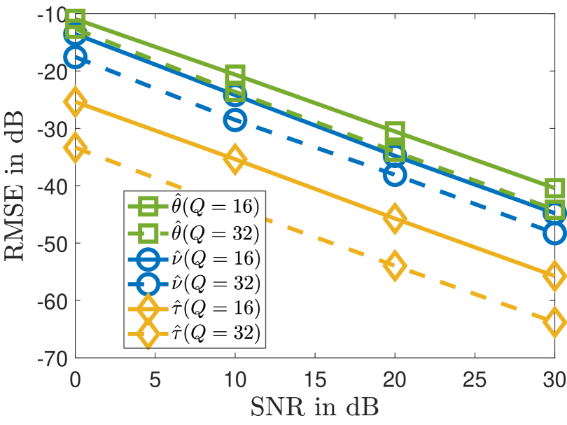
Figure 3: RMSE as a function of the number of subcarriers.

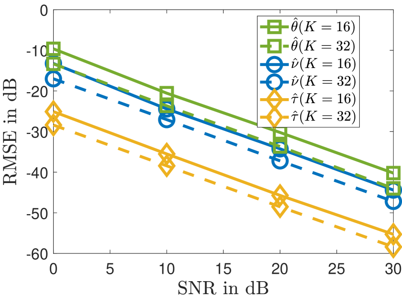
Figure 4: RMSE as a function of the number of blocks.

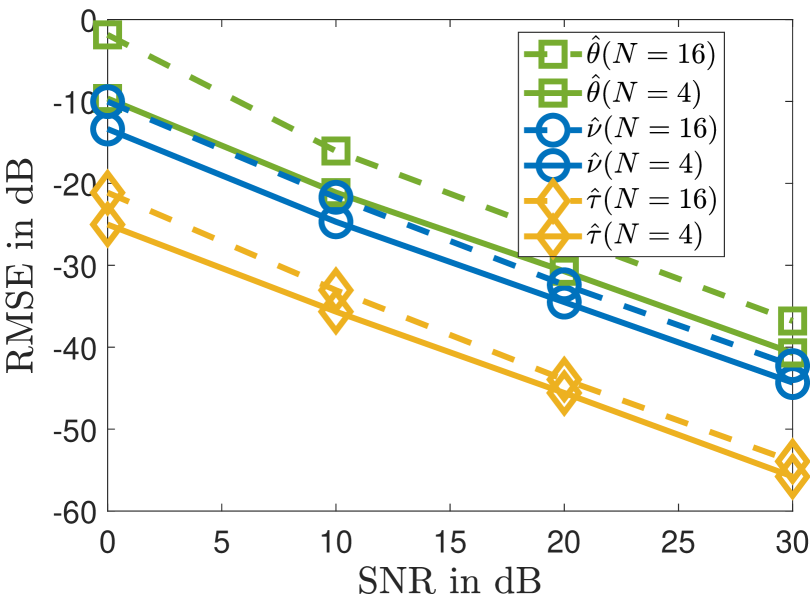
Figure 5: RMSE as a function of the number of RIS elements.

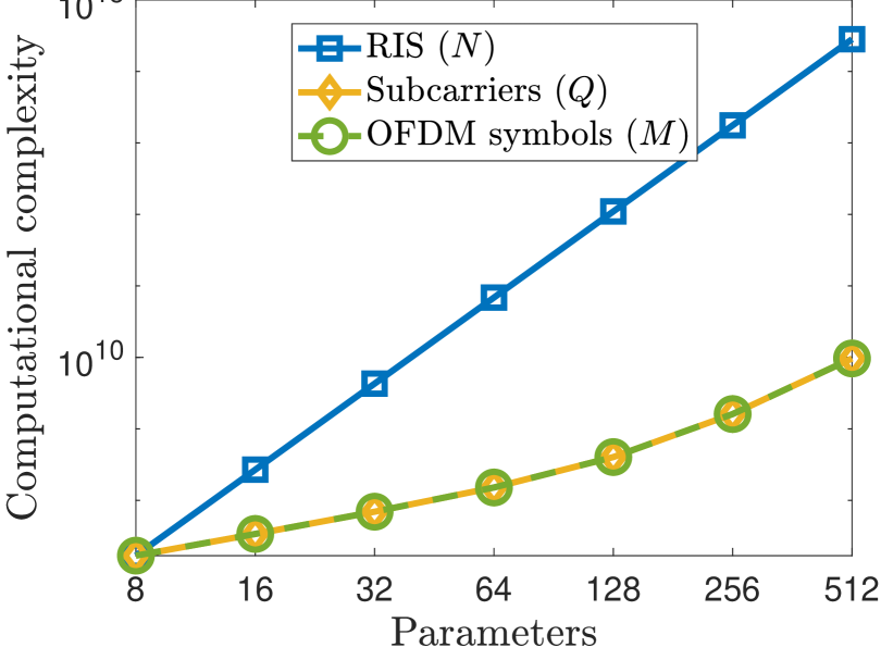
Figure 6: Computational complexity of Algorithm 1.

V Conclusion

We have proposed an NTBS model that fully exploits the intrinsic multidimensional nature of the received echo signal at the BS in a monostatic radar system, where the goal is to estimate the parameters of a single target. Our proposed NTBS algorithm estimates the delay, Doppler, and angle of the target using a two-stage ALS + ESPRIT approach. Our simulation results study the impact of the system parameters on the RMSE performance and complexity. Future work includes an extension of the NTBS algorithm to the multi-target scenario.

References

• [1] Q. Wu, S. Zhang, B. Zheng, C. You, and R. Zhang, “Intelligent reflecting surface-aided wireless communications: A tutorial,” IEEE Transactions on Communications, vol. 69, no. 5, pp. 3313–3351, 2021.
• [2] F. Liu, Y. Cui, C. Masouros, J. Xu, T. X. Han, Y. C. Eldar, and S. Buzzi, “Integrated sensing and communications: Toward dual-functional wireless networks for 6G and beyond,” IEEE Journal on Selected Areas in Communications, vol. 40, no. 6, pp. 1728–1767, 2022.
• [3] H. Zhang, H. Zhang, B. Di, K. Bian, Z. Han, and L. Song, “MetaRadar: Multi-target detection for reconfigurable intelligent surface aided radar systems,” IEEE Trans. Wireless Commun., vol. 21, no. 9, pp. 6994–7010, 2022.
• [4] M. Rihan, E. Grossi, L. Venturino, and S. Buzzi, “Spatial diversity in radar detection via active reconfigurable intelligent surfaces,” IEEE Signal Processing Letters, vol. 29, pp. 1242–1246, 2022.
• [5] X. Song, J. Xu, F. Liu, T. X. Han, and Y. C. Eldar, “Intelligent reflecting surface enabled sensing: Cramér-Rao bound optimization,” IEEE Transactions on Signal Processing, 2023.
• [6] X. Shao and R. Zhang, “Target-mounted intelligent reflecting surface for secure wireless sensing,” IEEE Trans. Wireless Commun., 2024.
• [7] M. Kemal Ercan, M. Furkan Keskin, S. Gezici, and H. Wymeersch, “RIS-aided NLoS monostatic sensing under mobility and angle-doppler coupling,” arXiv e-prints, pp. arXiv–2401, 2024.
• [8] K. B. A. Benício, B. Sokal, A. L. F. de Almeida, Fazal-E-Asim, B. Makki, and G. Fodor, “Low-complexity tensor-based monostatic sensing for IRS-assisted communication systems,” in Proc. 19th International Symposium on Wireless Communication Systems (ISWCS), 2024.
• [9] L. R. Ximenes, G. Favier, and A. L. de Almeida, “Semi-blind receivers for non-regenerative cooperative mimo communications based on nested parafac modeling,” IEEE transactions on signal processing, vol. 63, no. 18, pp. 4985–4998, 2015.
• [10] M. Tschudin, C. Brunner, T. Kurpjuhn, M. Haardt, and J. A. Nossek, “Comparison between unitary ESPRIT and SAGE for 3-D channel sounding,” in Proc. 49th IEEE VTC’99, vol. 2, 1999, pp. 1324–1329.
• [11] R. Feng, Y. Liu, J. Huang, J. Sun, and C.-X. Wang, “Comparison of MUSIC, unitary ESPRIT, and SAGE algorithms for estimating 3D angles in wireless channels,” in Proc. IEEE/CIC International Conference on Communications in China (ICCC), 2017.
• [12] Fazal-E-Asim, F. Antreich, C. C. Cavalcante, A. L. F. de Almeida, and J. A. Nossek, “Two-dimensional channel parameter estimation for millimeter-wave systems using Butler matrices,” IEEE Trans. Wireless Commun., vol. 20, no. 4, pp. 2670–2684, 2021.
• [13] P. Comon, X. Luciani, and A. L. F. de Almeida, “Tensor decompositions, alternating least squares and other tales,” Journal of Chemometrics, vol. 23, no. 7-8, pp. 393–405, 2009.
• [14] G. T. de Araújo, A. L. de Almeida, and R. Boyer, “Channel estimation for intelligent reflecting surface assisted mimo systems: A tensor modeling approach,” IEEE Journal of Selected Topics in Signal Processing, vol. 15, no. 3, pp. 789–802, 2021.
• [15] K. Benício, A. L. de Almeida, B. Sokal, B. Makki, G. Fodor et al., “Tensor-based modeling/estimation of static channels in IRS-assisted MIMO systems,” XLI Brazilian Symposium on Telecommunications and Signal Processing (SBrT), 2023.
• [16] K. B. Benício, A. L. de Almeida, B. Sokal, B. Makki, G. Fodor et al., “Tensor-based channel estimation and data-aided tracking in IRS-assisted MIMO systems,” IEEE Wireless Comms. Letters, 2023.
• [17] B. Sokal, M. Haardt, and A. L. F. de Almeida, “Semi-blind receiver for two-hop MIMO relaying systems via selective Kronecker product modeling,” in Proc. 8th IEEE CAMSAP’19, 2019, pp. 714–718.