How to quantify the coherence of a set of beliefs
Abstract.
Given conflicting probability estimates for a set of events, how can we quantify how much they conflict? How can we find a single probability distribution that best encapsulates the given estimates? One approach is to minimize a loss function such as binary KL-divergence that quantifies the dissimilarity between the given estimates and the candidate probability distribution. Given a set of events, we characterize the facets of the polytope of coherent probability estimates about those events. We explore two applications of these ideas: eliciting the beliefs of large language models, and merging expert forecasts into a single coherent forecast.
1. Introduction
When two or more predictions conflict, what is a principled way to combine them into a single meta-prediction?
This kind of question comes up in several different domains:
- •
-
•
A single individual may hold incoherent beliefs without being aware of the incoherence [5]. However, when someone points out that their beliefs are incoherent they may want to update to the “closest” coherent set of beliefs.
-
•
A market maker that has beliefs about underlying probabilities of events may want to give a coherent set of quotes so as to avoid giving a “Dutch book” that is exploitable via risk-free arbitrage [6].
-
•
The expressed opinions of a large language model can be very sensitive to small changes in the prompt. To investigate whether the model holds an internally coherent belief and extract that belief, one approach is to ensemble many weak predictors derived from the model’s internal state into a single meta-prediction [7].
Given a ground set , a list of events , and a list of credences , the vector is called coherent with respect to if there is a probability measure (on the Boolean algebra generated by ) such that for all .
For example, when predicting the next day’s weather, suppose three of our events are “rainy”, “warm and rainy”, “cold and rainy”. Then we have the coherence condition
If “warm or rainy” is also one of our given events , then we have the additional coherence condition
These two examples of coherence conditions are both the result of probabilities being overdetermined: fixing the probabilities of some events determines the probabilities of others. There is also a second kind of coherence condition that results from probabilities being between by 0 and 1. For example, even if “warm or rainy” is not one of our events, we still have the coherence condition
Given a list of events and credences we would like a systematic way of measuring incoherence: a loss function satisfying , with equality if and only if is coherent. One natural method of constructing such a loss is via some notion of “distance” from the vector to the set of coherent vectors:
| (1) |
We will discuss several choices of “distance” function . We write distance in quotation marks because need not be a metric (e.g. it might not be symmetric in and ).
The forecaster seeking to combine the beliefs of others (or individual seeking to correct their incoherent beliefs) can adopt the minimizer of (1). In Theorem 1 below we give conditions for existence and uniqueness of .
1.1. Plan of the paper
We start Section 2 defining the process of loss function minimization more precisely and giving conditions for when there is a unique minimizer . We proceed by summarizing a result from Predd et al. [8] that can motivate one’s choice of loss function and then by looking at two specific examples of loss functions (binary KL divergence and its transpose). We discuss natural justifications for these loss functions in Theorems 2 and 3.
Section 3 explores a possible application of our method to eliciting beliefs from large language models. We use loss functions to generalize the method suggested in [7] and consider possible modifications that this generalization allows.
Section 4 explores the geometry of , the set of coherent beliefs, which is a convex polytope. It is easy to describe the vertices of this polytope (Lemma 4.1), but somewhat more challenging to describe its facets (Theorem 4).
In Section 5, we consider how predictions should be aggregated in a setting where multiple experts each make internally coherent predictions. We seek a method to aggregate these predictions that leverages the internal coherence of each expert.
Finally, in Section F, we illustrate these methods in the scenario of masked letter prediction and discuss the results.
1.2. Related work
1.3. Preliminaries
We will assume that there are events for and that for each event , we receive some estimate of its probability. These estimates may come from a single expert or multiple experts. We discuss the implications of one expert giving multiple beliefs in Section 5.
Definition.
A credence base is the ordered pair where is a sequence containing the (potentially repeated) events whose probabilities are being estimated and is the vector whose th entry is .
Recalling that every finite Boolean algebra is the power set of a set, let be the Boolean algebra generated by , where is finite as is finite. For example, if then .
Definition.
A credence base is coherent if there exists a probability distribution where for all . We also call coherent with respect to if is coherent.
Definition.
The set of coherent beliefs over events is
2. Loss Functions that Quantify Incoherence
In this section, we examine a class of loss functions that are additive over events. We give conditions that guarantee that for any credence base there is a unique coherent credence base minimizing the loss . Then we state a theorem of Predd et al. [8] showing that in a certain forecasting setting it is never advantageous to submit an incoherent forecast. We proceed by giving natural justifications for two examples of loss functions: binary KL divergence and its transpose.
Recall that a function is lower semi-continuous at if
Also, we say that a function is strictly convex when finite if for all and in its domain, then
and the inequality is strict unless both sides are infinite.
Definition.
A dissimilarity function is a function satisfying
-
(i)
is lower semi-continuous with respect to
-
(ii)
is strictly convex when finite with respect to
-
(iii)
if and only if .
Some examples of dissimilarity functions are:
-
•
-
•
-
•
-
•
Given dissimilarity functions , we define an associated loss function given by
| (2) |
We typically consider all dissimilarity functions to be equal to some common . We denote the corresponding loss function and call it the loss function derived from dissimilarity function . We omit the subscript when it is clear from context.
Then, given a loss function with terms and a credence base with events, we can define the incoherence of to be
| (3) |
We denote the minimizing coherent belief by . The next theorem, which extends [9, Cor. 7] to a more general family of loss functions, gives conditions under which this minimizer is unique.
Theorem 1.
Given a credence base and a loss function of the form in (2), if there exists a coherent such that is finite, then there exists a unique such that
Moreover, if and only if .
Proof.
As the sum of lower semi-continuous and strictly convex when finite functions, is also lower semi-continuous and strictly convex when finite. Choose coherent such that is finite. As the set is compact, these is a sequence that converges to some so that
Then, by lower semi-continuity,
so is a minimizer of in .
As for uniqueness, if for ,
because and must be finite. Therefore, is not a minimizer of .
If , then by property (iii). Therefore, as can only take non-negative values and the minimizer is unique, .
∎
2.1. The coherence theorem of Predd et al.
The number is a way of quantifying the incoherence of the credence base . But which dissimilarity function should we use? One way to motivate the choice of arises from forecasting competitions: A forecaster submits a list of predicted probabilities for events , and these are scored after the outcomes of all events are known. If event occurred, then the forecaster receives penalty for that event; if did not occur, then the forecaster receives penalty for that event. The forecaster aims to minimize the expectation of the random variable
How should be chosen in order to elicit the true beliefs of each forecaster? If a forecaster believes that event will happen with probability , then the scoring rule should incentivize them to submit prediction in order to minimize their expected score. A function with this property is called a proper scoring rule. More formally, a proper scoring rule is a function satisfying [8, 11]:
-
(i)
For each , the quantity
is uniquely minimized at .
-
(ii)
is continuous in . Note that we allow to take the value , but ensures that all values of are finite except possibly and .
Predd et al. [8] prove that for any proper scoring rule , there is a dissimilarity function so that for any incoherent , the prediction using scores better than no matter which events actually happen! Namely, let
| (4) |
be the expected excess penalty for predicting rather than when the true probability of an event is . Note that for loss functions derived from such dissimilarity functions, we have with equality if and only if is coherent, because such functions are uniquely minimized when as is a proper scoring rule.
Theorem 2 ([8]).
Equation (4) still leaves a lot of possible choices of dissimilarity function , since there are many choices of proper scoring rule . Next we examine the case of the widely-used logarithmic scoring rule. The corresponding dissimilarity function turns out to be a variant of the Kulback-Leibler (KL) divergence [12].
2.2. Binary KL divergence
Capotorti, Regoli, and Vattari [9] proposed correcting incoherent probability assessments using the binary KL-divergence
| (5) |
The resulting loss can be interpreted as the total expected excess surprise of all experts, when expert predicts probability for event and the ground truth probability of is .
This loss function can also be motivated by the logarithmic scoring rule
with the goal to minimize total score . By Theorem 2, if is incoherent then the prediction using scores strictly better than the prediction no matter which events actually occur.
2.3. Transposed binary KL divergence
Next we consider the same loss with the roles of and interchanged:
In Table 1 we describe the coherent minimizer determined by and in each of two basic scenarios:
-
(1)
Partition: Fix and let . For all , we ;et . In this scenario all experts give estimates for different events, exactly one of which occurs.
-
(2)
Repetition: Let and for all , let . In this scenario all experts give estimates for the same event.
| Binary KL loss | Transposed binary KL loss | |
|---|---|---|
| Partition | does not depend on | does not depend on |
| Repitition |
The motivation for switching the order of the variables in comes from the following theorem, showing that the minimizer of loss functions determined by is now, in a certain scenario, the maximum likelihood estimation of .
Suppose the th expert independently observes some number of independent trials of event , and submits the estimate where is the number of trials in which occurred. Note that if , then has the binomial distribution .
To represent that each expert has a different amount of information, we can multiply each summand in (2) by some weight .
Theorem 3.
The maximum likelihood estimator given is
Proof.
The probability of receiving the estimations is
Next, if is the maximum likelihood estimation, then
3. Application: Eliciting Latent Beliefs from Language Models
Large language models sometimes express beliefs that they “know” to be false, for example because the prompt includes false statements. Burns et al [7] propose a method to elicit the model’s actual belief about a natural language claim corresponding to an event from its hidden state where is an assertion in natural language that the event holds. This method learns a linear probe minimizing the loss
| (6) |
where and are intended to estimate the model’s credence in the claims and . The idea is that the term is a measure of the incoherence of the linear probe, while the term encourages the linear probe to be decisive. We propose three possible elaborations of this approach, all of which train probes to minimize an expression of the form
where is a measure of incoherence and is a measure of indecisiveness.
3.1. The Case of a Single Event and its Complement
The following proposition shows that the measure of incoherence can be derived from the dissimilarity function .
Lemma 3.1.
When using dissimilarity function , the incoherence function becomes
Proof.
See Lemma D.1 in the appendix. ∎
This approach could be generalized to choosing to be either the functions or discussed previously. The next two lemmas give approximations for when is small
Lemma 3.2.
When using dissimilarity function
the loss function becomes
Proof.
See Lemma D.2 in the appendix. ∎
Lemma 3.3.
When using dissimilarity function
the loss function becomes
Proof.
See Lemma D.3 in the appendix. ∎
The reason that the term might be desirable to have in the denominator is that it increases the loss for the same absolute error when the probabilities are more extreme, which mirrors the intuition behind common scoring functions such as log-loss.
3.2. Multiple Probes and Multiple Events
A natural extension of [7] is to train probes where is trained to elicit the model’s credence from its th layer hidden state using rephrasings and of a natural language assertion about an event and its complement . Then, letting , one could replace the term of (6) with
This could be further generalized to a set of interrelated events each of which has natural language assertions that it holds, using the coherence term
Theorem 7 in Appendix C gives a formula for the gradient of assuming is sufficiently smooth.
Why would multiple probes () help elicit beliefs? We hypothesize that the language model’s beliefs – when they exist – arise from a bundle of internal heuristics that sometimes conflict. Each probe represents one such heuristic. In the case that is close to zero, the model’s internal heuristics are mostly self-consistent (the credences are close to an actual probability distribution) and in this case we might say that the model “has beliefs” about the claims . These beliefs could be certain or uncertain: if all the probes think a coin flip is 50% likely to land heads, then that is a coherent belief. On the other hand, if is large, then it is possible that the model “does not have beliefs” about the claims , or else that the probes simply did not discover the right heuristics.
Why would multiple events () help elicit beliefs? By minimizing applied to more events, we are encouraging not just but also and so on. The philosophy is that to find “beliefs”, one should look for functions of the hidden state that obey the laws of probability. The logical dependencies between events are incorporated in the definition of as a minimum over , as defined in equation (3). We further study the geometry of in Section 4.
3.3. Generalizing the Decisiveness Term
Recall that the term in Equation (6) is present to encourage the linear probe to be decisive. However, in the scenarios above with more than 2 estimates, it is unclear what should replace it. We discuss some options below:
-
•
We want the probes to be decisive so as to maximize information they give about the language model’s internal state. One way to quantify the information content of is by the maximum entropy of a probability distribution that gives . Hence, one could use the decisiveness term
where
-
•
The above notion can be generalized. Recall that is the log-loss scoring rule. Then, we can write entropy as
Recall that in Section 2.1, we discussed how a proper scoring rule can be transformed into a loss function . If using such a loss function, it might make sense to replace the log-loss function above with the proper scoring rule that is based on, making the decisiveness term
for a general proper scoring rule .
-
•
Using the idea that the least decisive distribution is the distribution that maximizes
let be this least decisive set of coherent beliefs and use either or to reward the probe for being more decisive.
-
•
When using or as a measure of dissimilarity, the incoherence term by itself might be enough to incentivize decisiveness due to the increased sensitivity of the sigmoid function to noise when its input is close to . To illustrate this, we revisit the scenario where we use one linear probe to find and from one natural language description of the event and one of its complement. We suppose that that the value of the linear probe has normal distribution and independently where is the probe’s goal credence in event . Regardless of which of or we choose as a dissimilarity function the expected value of the incoherence becomes approximately, using the quadratic approximation given by Lemmas 3.2 and 3.3:
Noting has mean and is the sum of two independent random variables with approximate variances by the -method, this becomes
As this is minimized when is close to or , the incoherence term by itself incentivizes the probe to be decisive.
4. The Polytope of Coherent Beliefs
Here, we explore the shape of the space of coherent beliefs. We first describe it as the convex hull of a finite set of -vectors in Lemma 4.1 and end by describing the inequalities that bound this polytope in Theorem 4.
Given a set of events with beliefs , let be the vector whose th entry is if and otherwise. Then, we can encode the structure of events in a matrix whose th row is the vector . Because contains the same information as , it will be convenient to use the pair to represent the credence base . We also encode a probability distribution on with the vector whose th entry .
Definition.
A vector is a probability vector if .
Lemma 4.1.
[9] A credence base is coherent if and only if is in the convex hull of the columns of .
Proof.
By definition is coherent if and only if there is a probability vector where . If is the th column of , that is true if and only if
For example, if we receive three beliefs: one about the probability of it being warm, one about the probability of it raining, and one of the probability of it being warm and raining, then the matrix becomes
So the polytope of coherent beliefs is the tetrahedron depicted in Figure 1.
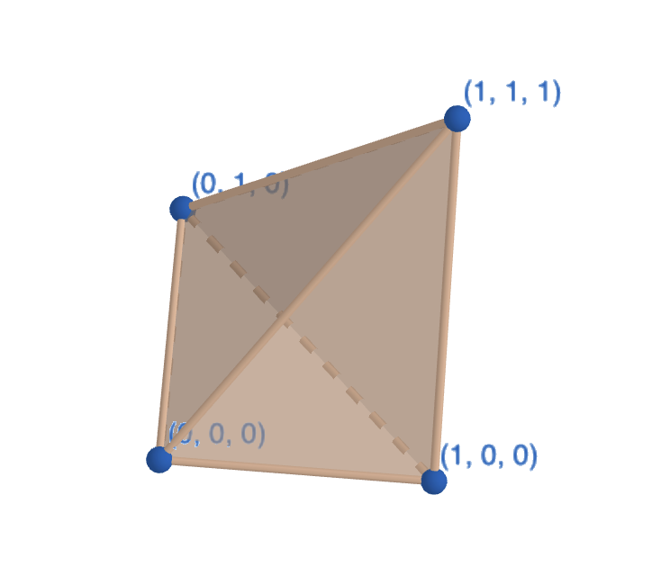
-
•
The facet not containing vertex corresponds to the inequality .
-
•
The facets not containing either or correspond to the inequalities and .
-
•
The facet not containing vertex corresponds to the inequality .
Let be the matrix obtained by appending a final row of s to . Similarly, take to have the same first entries as q and th entry and , the vector whose entries are all s. These represent the fact that . For two vectors , write if for all . Finally, let be and for a matrix , let denote the row span of .
The following is a statement of the Dutch Book Theorem [6].
Lemma 4.2.
The following are equivalent:
-
(i)
is coherent.
-
(ii)
For all , if , then .
Proof.
Suppose . By Farkas’ Lemma [13], as there is no with all entries in non-negative and , it must be that there is a solution to , with the row of s in ensuring that is a probability vector.
For the converse, consider coherent. Then, there exists where for all . But, if , then
as the dot product of two non-negative vectors. ∎
Lemma 4.3.
Suppose that for some non-zero vector where . Then, is incoherent.
Proof.
If , then we have but . By Lemma 4.2, is incoherent.
If , then , so is incoherent.
∎
Lemma 4.4.
Suppose that for some non-zero vector where . For any where , we can remove the th entry of and the th row from to obtain and so that the credence base is coherent if and only if is coherent.
Proof.
Without loss of generality, and . Call this vector . Consider removing the first entry of and the first row of to yield and .
For any where , if is is the vector with the first entry removed, then . Then, also . Therefore, if is coherent, then is coherent.
If were incoherent, then but , so is also incoherent.
∎
Based on Lemmas 4.3 and 4.4, from here on, we will only consider of rank . Then, as the rows of are linearly independent, the function where if is well-defined. By Lemma 4.2, is coherent if and only if for all .
Vectors can be thought of as “bets”, where the payout of the bet in world is equal to
where . We consider the bets to be against a bookmaker with credence base who expects no edge.
For such a bet , the vector represents the payout of atomwise: if atom happens, then the payout of bet will be . Because we assume that has full rank, there is a bijection between bets and atomwise payouts . Note that it does not make sense to talk about atomwise payouts outside of as it is impossible to make bets with such payouts.
For finding the coherence of a credence base, it is somewhat more helpful to think in terms of atomwise payouts rather than bets. For instance, if all entries of an atomwise payout are non-negative, then, if is coherent, the cost of the bet should be non-negative. The Dutch Book Theorem 4.2 tells us that having this condition for all atomwise payouts is equivalent to coherence. Recalling that the set of coherent beliefs is a polytope, each bet whose atomwise payout is non-negative corresponds to an inequality that all elements of the polytope satisfy, and if a belief is outside the polytope, it violates an inequality corresponding to some facet, which is a bet that can be made. The following lemma allows us to just consider a positive spanning set of atomwise payouts that need to be checked to ensure coherence.
Definition.
A positive spanning set of a set is a subset with the property that for any , there exist coefficients for each where only a finite number of are non-zero and
Lemma 4.5.
Let be a positive spanning set of . Then, is coherent if and only if for all .
Proof.
If , for some , then is incoherent by Lemma 4.2.
Suppose that for all . Then, consider any . As is a positive spanning set, we can represent
As is linear,
as the sum of the product of non-negative reals. Therefore, is coherent. ∎
Definition.
The set of extremal vectors of is
Let where we fix an arbitrary ordering of the finite number of entries of . We will show that is a minimal positive spanning set of .
If we think of each positive spanning set as a set of atomwise payouts that the bookmaker has to check is positive to ensure coherence, the following gives some atomwise payouts that the bookmaker definitely has to check.
Lemma 4.6.
Let be a positive spanning set of where . Then,
Proof.
If did not include such a , as is a positive spanning set, then there is a finite set where for some . But as not all , without loss of generality, suppose . Then, , so . As the first non-zero entry of each is , . ∎
Definition.
Let be a subset of . Consider where . A vector is maximally- in if there there is no where .
Lemma 4.7.
For any vector that is maximally- in , if for some vector , then .
Proof.
Suppose that . Let the first non-zero entry of be and the first non-zero entry of be . Then, and . ∎
It turns out that it suffices to just check the maximally-0 elements of , as shown by the following to lemmas.
Lemma 4.8.
A vector is maximally- in if and only if .
Proof.
Suppose that . Then, there exists where . Then, , so by Lemma 4.7, is not maximally-0 in .
Suppose that . If were not maximally- in , then we would have with with . Let be the maximum entry of and be the minimum entry of . Then, , which is impossible as cannot be in the span of by the definition of . Therefore, is maximally- in by contradiction.
Next, it suffices to show that if is maximally- in , then is maximally- in . To see this, suppose not and that there exists some , where . Then, and . But and we have , which contradicts the fact that is maximally- in .
∎
Lemma 4.9.
is a positive spanning set of .
Proof.
For the sake of contradiction, suppose that is not a positive spanning set and consider to be a maximally- vector not its positive span. As is not in the span of any element of , is not maximally- in . Therefore, there exists where . For all non-zero elements of , consider and let . Then, , so as , is in the positive span of . For , let and . Then, and . Therefore, and are both elements of the positive span of , so must also be an element of the positive span of . ∎
Theorem 4.
The hyperplane is a facet of the polytope whose vertices are the columns of if and only if
Proof.
By [14], the hyperplane is a facet of a polytope if and only if for all vertices of , with equality for a maximal subset of vertices. This happens if and only if the vector
with equality for a maximal subset of the entries, which is true if and only if
and is maximally- among vectors in . By Lemma 4.8, this is equivalent to . ∎
Corollary.
There is a one to one correspondence between elements of and facets of the polytope whose vertices are the columns of .
By [14], every non-redundant set of inequalities bounding a polytope has exactly one inequality for every face. This means that if a bookmaker verifies that they are not giving a Dutch book by checking a fixed set of inequalities, it suffices to check the inequalities for all , and every non-redundant set of inequalities they must check consists of rescaled versions of these inequalities.
5. Merging Individually Coherent Experts
In this section we consider a setting in which each of several experts submits a set of internally coherent credences, but the union of all expert credences is possibly incoherent. To aggregate these credences into a single coherent set of beliefs, we could use a loss function of the form (2), but that ignores the additional information that beliefs from the same expert are coherent. Since logical inferences can be made from an expert’s stated credences, the expert can express the same information in multiple ways. As long as the set of possible inferences about an expert’s beliefs is the same, the loss function should be invariant under the specific information the expert shares, a property that the method for separate beliefs previously discussed does not have if naively applied here. We call this property content invariance and discuss it further below.
For example, if a meteorologist says that there is a chance of rain tomorrow and a chance of clouds, it is reasonable to infer that there is a chance of sun and a chance of clouds without rain. In such a situation, the meteorologist might also explicitly say the chance of it being sunny, however, because that statement does not provide new information, the loss function should be invariant under whether or not they say it.
Recall that obtained by appending a row of s to and that is the row span of .
Definition.
Two coherent credence bases and are content equivalent if and the credence base is coherent.
Lemma 5.1.
If and are content equivalent and is a probability vector, then
Proof.
Since , the orthogonal space to the row span of , if , then . By the coherence of , there is some so that and . Then, for any probability vector , as ,
Lemma 5.1 implies that content equivalence is transitive, so is an equivalence relation.
Definition.
Let be a function of a credence base. is content invariant if for content equivalent credence bases and we have .
5.1. Content Invariance
Suppose that is a coherent credence base where the rows of are linearly independent. Let , which the next lemma shows is the set of events whose probabilities are linearly inferable.
Lemma 5.2.
Consider the statements
-
(i)
.
-
(ii)
There is a unique belief so that the credence base is coherent.
(i) implies (ii). Moreover, if there is a probability vector so that where none of the entries of are or , then (ii) implies (i).
Proof.
Suppose (i). The belief makes coherent as is coherent. For uniqueness, suppose we there are two coherent beliefs about some event for . Then as there is some where , there are two probability vectors and where and with . This means that
Suppose not (i) and let be the matrix with the vector appended as the last row. Then, there is a vector . By the assumption that no entries of are or , there is an so that for all , is also a probability vector. Then, for all such , taking makes coherent. As , we have , so each distinct value of yields a distinct . ∎
Lemma 5.3.
Let be the reduced row-echelon form of . Then,
Proof.
Firstly,
Note that all of ’s columns have a leading which is the only entry in its row, so each of ’s entries appear somewhere in . Therefore, if , then . ∎
Corollary.
The maximum size of is .
Because is defined only in terms of the row span , it is content invariant. However, tends to be quite large even for well-tamed events, so a smaller, content invariant set might be desirable.
Let be a minimal positive spanning set of .
Lemma 5.4.
Any maximally- element of must be part of .
Proof.
Suppose that is maximally- in . As is a positive spanning set, we can write
As , there is some where , so and . As is maximally-, which means that as both are -vectors. ∎
Theorem 5.
is the set of maximally- elements of .
Proof.
It suffices to show that the maximally- elements of are a positive spanning set. Suppose that this were not the case. Let be a maximally- vector in , the maximal set positively spanned by . Note that is not maximally- in or it would be a member of . Then, there exists where . Note that , meaning and are both in the positive span of , so is also in the positive span of . ∎
Lemma 5.5.
Let be the implied belief function, taking an event to the unique belief that makes the credence base coherent. The function as well as the sets and are content invariant.
Proof.
Let and be two content equivalent coherent credence bases with set of inferable events and , positive bases and of and , and implied belief functions and . Then, by definition, , so is content invariant. Also, because and are defined solely in terms of and respectively, .
To show that is content invariant, if , then by coherence, there is a probability vector so that and . By Lemma 5.1, we have , meaning that certifies that is coherent, so by uniqueness, .
∎
5.2. Loss Functions with Content Invariance
Suppose that there are experts, the th of which tells us the coherent credence base of their beliefs , with event matrix and belief vector defined previously. Let be the combined credence base of all experts, formed by concatenating and . We will consider loss functions of the form
for some content invariant measure of disagreement . In contrast to Section 2, the sum is over experts rather than over individual events. As before,
is a measure of the incoherence of the set of experts as a group.
For the th expert, let be the set of events for which we can infer a probability from expert ’s stated beliefs, let be this inferred probability, and let be the minimal positive spanning set of , as defined in Section 5.1. Also, write be the entry of corresponding to event .
As is content invariant one approach is to let
| (7) |
where is a content invariant set of events and is a dissimilarity function as in Section 2. As and are both content invariant, they are both choices for .
One possible justification for summing over instead of is that can be much larger than . contains the maximally- elements of , or the elements whose probabilities are smallest. As the dissimilarity functions and punish more for the same error when is smaller (), summing over is summing over the elements of whose relative errors will be greatest while not considering the other terms for ease of computation.
The normalizing coefficient is included in the loss function in order to give each expert equal weight, regardless of how many beliefs they express. If the measures of disagreement were not normalized, then an expert might become twice as influential on the overall loss function by expressing one additional belief because and can grow exponentially with the number of beliefs expressed.
5.3. Removing the Symmetry between an Event and its Complement
Looking at the dissimilarity function , there are two terms: representing the expected surprise from the event occurring and , representing the expected surprise from the event not occurring. However, if we sum the dissimilarity function over a minimal positive basis, then being surprised by the complement of an event happening is redundant; when one event does not happen, we are surprised instead by other events happening. Alternatively, an agent observing the world might only keep track of which events do happen, so cannot be surprised by an event not happening.
This motivates the removal the term representing the surprise of an event not happening from the loss function. However, one needs to be careful in doing this: so far, we have required that loss functions be non-negative and equal to if and only if . For example, by itself is not a dissimilarity function, so the corresponding “loss function” does not have this property in general. The following lemmas motivates two possible content invariant disagreement functions that have this property:
Lemma 5.6.
Let and be coherent credence bases and suppose that for some . Then,
with equality if and only if .
Proof.
Recall from Section 2.1 that for a proper scoring rule , there is an associated dissimilarity function . When using the log-loss scoring rule, this becomes . Can we generalize Lemma 5.6 to apply to half-dissimilarity functions
| (8) |
for a proper scoring rule ? No. The following lemma shows that log-loss is the only differentiable proper scoring rule for which Lemma 5.6 holds.
Lemma 5.7.
Let be a proper scoring rule that is differentiable in for with as defined in equation (8). Suppose that for all coherent credence bases where for some ,
Then for some and ,
Proof.
Note that by continuity, the value of when are determined by its values on the interval . Write
Let be the identity matrix and let where is the derivative of in . For any , consider the coherent belief vector . By the assumption that is minimized among coherent when , Lagrange multipliers yield that
so for all . For , take to be the identity matrix and . The same argument as above shows that . Therefore, for all , we have , so and for some .
As is a proper scoring rule, the quantity is uniquely minimized in when , so , meaning that and for some . Therefore, we have
In order for to be a proper scoring rule, we must have . ∎
Acknowledgements
We thank Kenny Easwaran, Jonathan Gabor, Oliver Hopcroft, David Krueger, Yuval Peres, Suvadip Sana, Luchen Shi, and Ariel Yadin for inspiring discussions.
References
- [1] Francis Galton “Vox Populi” Number: 1949 Publisher: Nature Publishing Group In Nature 75.1949, 1907, pp. 450–451 DOI: 10.1038/075450a0
- [2] Lyle H. Ungar et al. “The Good Judgment Project: A Large Scale Test of Different Methods of Combining Expert Predictions” In AAAI Fall Symposium: Machine Aggregation of Human Judgment, 2012
- [3] Nuño Sempere and Alex Lawsen “Alignment Problems With Current Forecasting Platforms”, 2023 arXiv:2106.11248 [cs.GT]
- [4] Thomas McAndrew, Nutcha Wattanachit, Graham C. Gibson and Nicholas G. Reich “Aggregating predictions from experts: a review of statistical methods, experiments, and applications” In Wiley interdisciplinary reviews. Computational statistics 13.2, 2021, pp. e1514 DOI: 10.1002/wics.1514
- [5] Stefan M. Herzog and Ralph Hertwig “Harnessing the wisdom of the inner crowd” In Trends in Cognitive Sciences 18.10, 2014, pp. 504–506 DOI: 10.1016/j.tics.2014.06.009
- [6] R. Lehman “On Confirmation and Rational Betting” In The Journal of Symbolic Logic 20.3 [Association for Symbolic Logic, Cambridge University Press], 1955, pp. 251–262 URL: http://www.jstor.org/stable/2268221
- [7] Collin Burns, Haotian Ye, Dan Klein and Jacob Steinhardt “Discovering Latent Knowledge in Language Models Without Supervision”, 2022 arXiv:2212.03827 [cs.CL]
- [8] Joel B. Predd et al. “Probabilistic Coherence and Proper Scoring Rules” Conference Name: IEEE Transactions on Information Theory In IEEE Transactions on Information Theory 55.10, 2009, pp. 4786–4792 DOI: 10.1109/TIT.2009.2027573
- [9] A. Capotorti, G. Regoli and F. Vattari “Correction of incoherent conditional probability assessments” In International Journal of Approximate Reasoning 51.6, 2010, pp. 718–727 DOI: 10.1016/j.ijar.2010.02.002
- [10] Matthias Thimm “Inconsistency measures for probabilistic logics” In Artificial Intelligence 197, 2013, pp. 1–24 DOI: 10.1016/j.artint.2013.02.001
- [11] Robert L. Winkler and Allan H. Murphy “‘Good’ Probability Assessors” Publisher: American Meteorological Society In Journal of Applied Meteorology (1962-1982) 7.5, 1968, pp. 751–758 URL: https://www.jstor.org/stable/26174473
- [12] S. Kullback and R.. Leibler “On Information and Sufficiency” Publisher: Institute of Mathematical Statistics In The Annals of Mathematical Statistics 22.1, 1951, pp. 79–86 DOI: 10.1214/aoms/1177729694
- [13] Julius Farkas In Journal für die reine und angewandte Mathematik (Crelles Journal) 1902.124, 1902, pp. 1–27 DOI: doi:10.1515/crll.1902.124.1
- [14] Günter M. Ziegler “Lectures on 0/1-Polytopes” In Polytopes — Combinatorics and Computation Basel: Birkhäuser Basel, 2000, pp. 1–41 DOI: 10.1007/978-3-0348-8438-9˙1
- [15] M. Cover and Joy A. Thomas “Elements of Information Theory” Wiley Interscience, 2005
- [16] Sébastien Bubeck “Convex Optimization: Algorithms and Complexity” In Foundations and Trends in Machine Learning 8.3-4, 2015, pp. 231–357 DOI: 10.1561/2200000050
- [17] Eric Price “Wordlist 10000” URL: https://www.mit.edu/~ecprice/wordlist.10000
Appendix A Numerical Comparison between and
To contrast the two settings in Section 2: One should use the dissimilarity function when submitting multiple forecasts based on their possibility incoherent internal beliefs (and expects these forecasts to be scored with the logarithmic proper scoring rule); its transpose should be used in aggregating independent sources of information, each of which gives information about one event, in order to find the most likely true probability distribution.
Recall that is the vector whose th entry is if and otherwise. Additionally, denotes the th standard basis vector and 1 the vector of all s. For any distribution , we associate a vector with it, whose th entry is , the probability of the th atom in the Boolean algebra.
Table 2 contains some examples of the numerical differences between using and as dissimilarity functions.
| Situation | ||
|---|---|---|
| Exactly one event occurs: | ||
| All estimates are for the same event: | ||
| , | ||
| , | ||
| , | ||
| , | ||
| , | ||
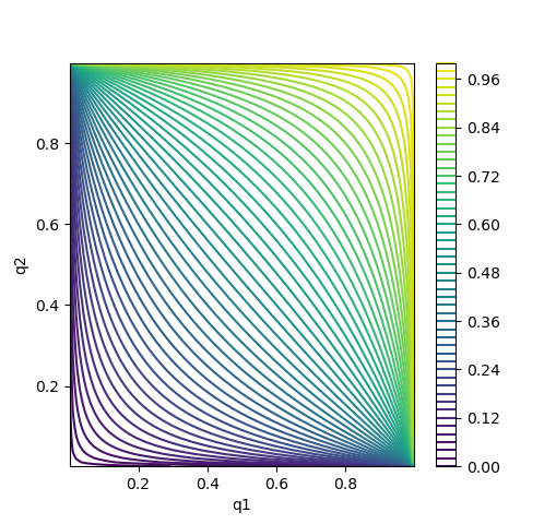
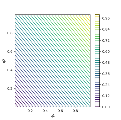
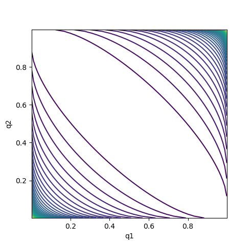
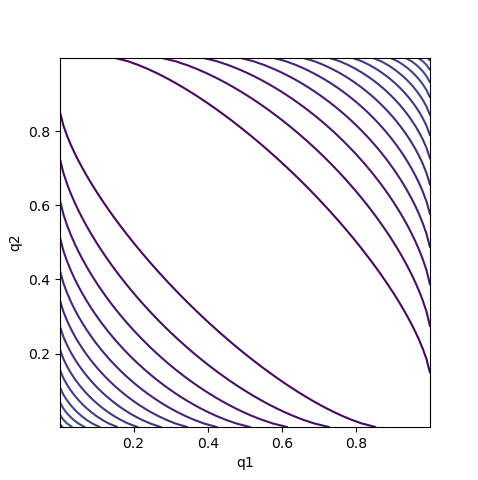
The differences in and also leads the function to behave differently when using the two functions, as illustrated in Figure 3, where and are the events being estimated.
Appendix B Computing and
One way to find and numerically is to define a function that, given a vector and the matrix whose th row is , and the credences , returns . Then, one can use a gradient descent algorithm to minimize under the conditions that the entries of are nonnegative and sum to . This algorithm is illustrated below in psuedocode.
Computing to within an accuracy of takes time [16]. Python code to compute and can be found on https://github.com/scim142/quantifying_coherence.
Appendix C Holder Continuity of and
Let denote the Euclidean norm.
Lemma C.1.
If is (strictly) convex/-times differentiable/Lipschitz in //both, then will also be.
Proof.
(convexity in ) Let . Then, for ,
so is convex. As is the sum of convex functions, is convex. ∎
Lemma C.2.
If is Lipchitz in in some region , then will be Lipchitz on the set with Lipschitz constant equal to that of in .
Proof.
Let and consider the case when . Let and be the Lipschitz constant of . Then,
If , then the above shows that . Therefore, regardless of the relative sizes of and , we have
Lemma C.3.
If is strictly convex and twice differentiable in , then is continuous.
Proof.
Fix any and , greater than the Lipschitz constants of with respect to and respectively in the neighborhood of . Let be a closed region in which is Lipschitz in with Lipschitz constant and Lipshcitz in with Lipschitz constant and be a closed region contained in that contains .
Let be a sequence in with limit . As for all , and is sequentially compact, the sequence has a subsequence with a limit. Let be one of those limit and be a subsequence of where the limit of is . Then, for any , there exists where for all , and . Then, by Lemma C.2,
Using the fact that is Lipschitz in and , by the triangle inequality
As this is true for all , we must have , so by Theorem 1, and is continuous at .
∎
Let be the gradient of with respect to at .
Theorem 6.
If is strictly convex and twice differentiable in , then is Holder-.
Proof.
Fix any and let be the least eigenvalue of the Hessian of with respect to at , let be some open region over which is Lipschitz that contains , and let . Additionally, let be the Lipschitz constant of with respect to on . Then, first of all, by Lemma C.2, for all where ,
Then, by the triangle inequality, as is Lipschitz in
So,
Also, as is twice differentiable in and is continuous at by Lemma C.3,
where and as in Theorem 1. Then, for any , for there exists where for
So
And is Holder- in the open ball of radius at . ∎
Let be the gradient of as is changed at the point .
Theorem 7.
Suppose there is some open region where is Holder- for some , and is twice differentiable at for . Then, is differentiable in with derivative .
Proof.
Let be the Holder- coefficient of and the least eigenvalue of the Hessian of with respect to at . Then, consider
as and are both continuous. Then,
Note that by the minimum property of
So,
and . ∎
Appendix D Proofs of Section 3.1
Lemma D.1.
When using dissimilarity function , the loss function becomes
Proof.
Lagrange multipliers yield . Therefore
Lemma D.2.
When using dissimilarity function
the loss function becomes
Proof.
Lagrange multipliers yield that the closest coherent probability satisfies , giving the loss
Letting and be the odds of derived from the two probes with and the probabilities derived from the probes and Taylor expanding in about yields:
Lemma D.3.
When using dissimilarity function
the loss function becomes
Proof.
Again letting and , Lagrange multipliers show that , which we will denote by for ease of notation. Taking the derivative of in gives
and
Then, Taylor expanding around in gives
Appendix E Comparison of Expert Aggregation Methods
Here, we will look at the following scenario and consider what various methods from Section 5 give us as estimates of the probabilities of various events:
We take and consider two experts. The first expert submits probability estimates for two events
and the second expert submits estimates for three events
Table 3 summarizes the aggregated beliefs using four different methods and two different dissimilarity functions.
| Aggregation Method | with | with | ||
|
Sum over stated beliefs only (not content invariant):
|
||||
|
Sum over all inferable beliefs:
|
||||
|
Sum over the minimal positive basis:
|
||||
|
Sum over the minimal positive basis, asymmetric variant:
|
It should be noted that the first method assigns a probability of to atom , but that it is given non-zero probability by all the content invariant methods. This is because the event is not present in the sum over stated beliefs only, but is present in all the other sums.
Appendix F Extended Example: Masked Letters
We illustrate the methods of Section 5 in the following scenario: given a word with one masked letter, we seek to predict the masked letter by combining two heuristics, which will play the role of experts in Section 5. One heuristic uses the preceding letters to make predictions and the other heuristic uses the succeeding letters to make its predictions.
For example, given the word EM*IL, with the third letter masked, the first expert would use the 3-gram EM* to make its predictions . The second heuristic would use the 3-gram *IL to make the predictions .
If each heuristic is derived from counting 3-gram frequencies in a corpus, then it will be internally coherent, so we use a content invariant loss function as outlined in Section 5. As , the size of the set of events whose probabilities can be inferred, is much too large, one should either sum over the minimal spanning sets or sum over subsets of the minimal spanning sets that add to . We will outline the calculations using dissimilarity function and compare the results with .
F.1. Method 1: Summing over a Positive Basis
Here we consider the loss function determined by
Recall that is the normalizing constant, equal to the number of terms in the summand. Additionally, in this situation, the heuristics’ predictions are exactly the minimal spanning set. So
Then, if all entries in are strictly positive (which they will be for and as long as all entries in and are non-zero), by Lagrange multipliers as , there is some constant where for all
Taking and calculating shows
so
does not depend on . Computing analytically from here is difficult, so some numerical algorithm should be used.
F.2. Method 2: Using an Asymmetric Loss Function
Here we consider the loss function determined by
Here is the set of subsets of whose sum is . In this case, is the singleton set as the heuristic’s predictions are the maximal spanning set and their sum is , so we sum over the same events as previously. However, instead of using the function , we use and ignore the terms related to the surprise of a letter not being chosen. As is the number of terms in the summand, the loss function is
As we are using , so , this becomes
And again using Lagrange multipliers to take the derivative, the quantity
does not depend on . Therefore, for some that does not depend on ,
Using the fact that ,
F.3. Comparison of Methods
Using a list of 10,000 common English words [17], there are 7 letters that appear both after EM and before IL, not necessarily in the same word (A, B, E, M, O, P, S). Applying the methods described above yields Table 4:
| Letter | |||||
|---|---|---|---|---|---|
| with | with | ||||
Firstly, in this setup, when using , it does not matter whether one includes the terms. In either case, the method amounts to setting , which is coherent as the set of coherent beliefs is convex. This will not always be the case, and was so here because of the simplicity of the events included in the sum. Looking at the results of using , there is little difference, although low probabilities () seem to be given more weight when excluding terms. As usual, gives more extreme estimates than with either method.
Here, both methods with either loss function were correct in assigning the letter A the highest probability in EMAIL. However, this is not usually the case. Over all the 5 letter words in [17], both methods using gave the highest probability to the actual letter about of the time and both methods using were correct about of the time. The code to reproduce this experiment can be found at https://github.com/scim142/quantifying_coherence.