Quaternion-based Unscented Kalman Filter for 6-DoF Vision-based Inertial Navigation in GPS-denied Regions

Abstract

This paper investigates the orientation, position, and linear velocity estimation problem of a rigid-body moving in three-dimensional (3D) space with six degrees-of-freedom (6 DoF). The highly nonlinear navigation kinematics are formulated to ensure global representation of the navigation problem. A computationally efficient Quaternion-based Navigation Unscented Kalman Filter (QNUKF) is proposed on $\mathbb{S}^{3}\times\mathbb{R}^{3}\times\mathbb{R}^{3}$ imitating the true nonlinear navigation kinematics and utilize onboard Visual-Inertial Navigation (VIN) units to achieve successful GPS-denied navigation. The proposed QNUKF is designed in discrete form to operate based on the data fusion of photographs garnered by a vision unit (stereo or monocular camera) and information collected by a low-cost inertial measurement unit (IMU). The photographs are processed to extract feature points in 3D space, while the 6-axis IMU supplies angular velocity and accelerometer measurements expressed with respect to the body-frame. Robustness and effectiveness of the proposed QNUKF have been confirmed through experiments on a real-world dataset collected by a drone navigating in 3D and consisting of stereo images and 6-axis IMU measurements. Also, the proposed approach is validated against standard state-of-the-art filtering techniques.

For video of navigation experiment visit: link
For video of navigation experiment comparison visit: link
 

I Introduction

I-A Motivation

Navigation is generally defined as the process of determining the position, orientation, and linear velocity of a rigid-body in space, performed by either an observer or external entities. Navigation, both in its complete and partial forms, plays a crucial role in numerous systems and fields, significantly improving operational performance and efficiency. Its applications range from robotics to smartphones, aerospace, and marines [1, 2], highlighting its vital importance in driving technological and scientific progress. In the smartphone industry, the precise estimation of a pedestrian’s position and heading through their mobile device is essential for improving location-based services and facilitating seamless navigation between outdoor and indoor environments. Advancing accuracy and reliability of the estimation is critical for enriching user experiences in wayfinding applications, as documented in recent studies [3, 4, 5, 6, 7]. In aerospace, the precise estimation of satellite orientation is pivotal for the functional integrity of satellites, particularly for the accurate processing of observational data. This aspect is fundamental to ensuring the reliability and effectiveness of satellite operations [8, 9, 10].

Autonomous and unmanned robots employ navigation techniques to enhance the precision of Global Navigation Satellite System (GNSS)-based localization systems, such as the Global Positioning System (GPS) and GLONASS. These enhancements are critical for ensuring operational functionality in environments where GPS signals are obstructed or unavailable [5, 11]. This capability is particularly vital for Unmanned Aerial Vehicles (UAVs) navigating indoors or within densely constructed urban areas, where direct line-of-sight to satellites is frequently obscured. Navigation methods that do not rely on GNSS hold significant importance in maritime contexts, where GNSS signals can be unreliable or entirely absent, especially in deep waters or in the vicinity of harbors [12]. Such GNSS-independent navigation techniques are crucial for ensuring the safety and efficiency of marine operations, where traditional satellite-based positioning systems may not provide the necessary accuracy or reliability.

I-B Related Work

A naive approach to localizing an agent in a GNSS-denied environment is to apply Dead Reckoning (DR) using a 6-axis Inertial Measurement Unit (IMU) rigidly attached to the vehicle and comprised of an accelerometer (supplying the apparent acceleration measurements) and a gyroscope (supplying angular velocity measurements) [5, 1]. DR is able to produce the vehicle navigation state utilizing gyroscope measurements and integration of acceleration provided that initial navigation state is available [13, 5]. DR is widely utilized for pedestrian position and heading estimation in scenarios where GNSS is unreliable (e.g., indoor environments). Typically, the step count, step length, and heading angle are each determined by an independent sensor, and these measurements are then incorporated into the last known position to estimate the new position. This method serves as a preprocessing step for the DR, and aims to enhance the accuracy of heading estimation. However, a major limitation of DR is the accumulation of errors in the absence of any measurement model, leading to drift over time. In the pedestrian DR domain, multiple solutions have been proposed to mitigate the drift issue, such as collection of distance information from known landmarks, a deep-learning based approach to supply filtered acceleration data [6], Recurrent Neural Network (RNN) with adaptive estimation of noise covariance [14] and others. These approaches are subsequently coupled with a Kalman-type filter to propagate the state estimate. However, these methods, while enhancing the robustness of the filter, fail to correct the state estimate if significant drift occurs.

In scenarios where a robot navigates in a known environment, leveraging measurements from the environment can be a solution to the drift problem encountered by the pure IMU-based navigation algorithms. Ultra-wideband (UWB) has recently gained popularity as an additional sensor in the navigation suite. A robot equipped with a UWB tag gains knowledge of its positions by communicating with fixed UWB anchors with known positions [15, 2, 16, 17, 18]. This is beneficial for structured environments with sufficient fixed reference points (e.g., ship docking [17] and warehouse [15]). However, the need for infrastructure with known fixed anchors limits the generalizability of UWB-based navigation algorithms in unstructured regions [3]. With advances in three-dimensional (3D) point cloud registration and processing technologies, such as the Iterative Closest Point (ICP) [19] and Coherent Point Drift (CPD) [20], the dependency on initial environment knowledge is significantly reduced. Utilizing these algorithms, a robot equipped only with its perspective of 3D points at multiple steps can reconstruct the environment. This reconstructed environment then is treated as known, allowing the feature points obtained from the environment to serve as independent measurements alongside the IMU [1, 21]. Technologies such as Sound Navigation And Ranging (SONAR), Light Detection And Ranging (LIDAR), and visual inputs from mono or stereo cameras exemplify such measurements. SONAR and LIDAR sensors emit mechanical and electromagnetic waves, respectively, and construct 3D point clouds by measuring the distances that each wave travels. SONAR is a popular sensor in marine applications [22], as water propagates mechanical waves (sound waves) significantly better than electromagnetic waves (light waves). LIDAR is commonly used in space application [23] since sound waves cannot propagate through space while light can. However, both LIDAR and SONAR struggle in complex indoor and urban environments due to their inability to capture colour and texture. Therefore, vision-based aided navigation (stereo or monocular camera + IMU) has emerged as a reliable navigation alternative for GPS-denied regions. In particular, modern UAVs are equipped with high-resolution cameras which are more cost-effective and computationally reliable.

I-C Vision-based Navigation and Contributions

Feature coordinates in 3D space can be extracted using a monocular camera (given a sequence of two images with persistent vehicle movement) or a stereo (binocular) camera [5, 24]. While stereo vision-based navigation algorithms, such as those proposed in [25] and [26], generally outperform monocular-based systems, they encounter difficulties in dark environments and in absence of clear features, such as a drone facing a blank wall. Fusing data from IMUs and vision sensors is a widely accepted solution to address navigation challenges, as these modalities complement each other [5, 27, 28, 29]. This integration of vision sensors and IMU is commonly referred to as Visual-Inertial Navigation (VIN) [30]. Kalman-type filters have been extensively used to address the VIN problem due to their low computational requirements and ability to handle non-linear models via linearization. An early significant contribution in this area was made by Mourikis et al. [29], who developed a multi-state Kalman filter-based algorithm for a VIN system that operates based on the error state dynamics. This approach allows the orientation, which has three degrees of freedom, to be represented by a three-dimensional vector. To address the issue of computational complexity and expand the algorithm proposed in [29], the work in [31] explored various methods for fusing IMU and vision data using the Extended Kalman Filter (EKF). Specifically, they examined the integration of these data sources during the EKF prediction and update phases. Although EKF is an efficient algorithm, its major shortcoming is the use of local linearization which disregards the high nonlinearity of the navigation kinematics. Therefore, there is a need for multiple interacting models to tackle EKF shortcomings [32]. Moreover, EKF is designed to account only for white noise attached to the measurements, making it unfit for measurements with colored noise [8].

Contributions

Unscented Kalman Filter (UKF) generally outperforms the EKF [8] since it can accurately capture the nonlinear kinematics while handling white and colored noise [8, 33]. Motivated by the above discussion, the contributions of this work are as follows: (1) Novel geometric Quaternion-based Navigation Unscented Kalman Filter (QNUKF) is proposed on $\mathbb{S}^{3}\times\mathbb{R}^{3}\times\mathbb{R}^{3}$ in discrete form mimicking the true nonlinear navigation kinematics of a rigid-body moving in the 6 DoF; (2) The proposed QNUKF is tailored to supply attitude, position, and linear velocity estimates of a rigid-body equipped with a VIN unit and applicable for GPS-denied navigation; (3) The computational efficiency and robustness of the proposed QNUKF is tested using a real-world dataset collected by a quadrotor flying in the 6 DoF at a low sampling rate and subsequently compared to state-of-the-art industry standard filtering techniques.

I-D Structure

The remainder of the paper is organized as follows: Section II discusses preliminary concepts and mathematical foundations; Section III formulates the nonlinear navigation kinematics problem; Section IV introduces the structure of the novel QNUKF; Section V validates the algorithm’s performance using a real-world dataset; and Section VI provides concluding remarks.

II Preliminaries

TABLE I: Nomenclature

$\left\{\mathcal{B}\right\}$ / $\left\{\mathcal{W}\right\}$	:	Fixed body-frame / fixed world-frame
$\mathbb{SO}\left(3\right)$	:	Special Orthogonal Group of order 3
$\mathbb{S}^{3}$	:	Three-unit-sphere
$\mathbb{Z}$, $\mathbb{Z}^{+}$	:	Integer and positive integer space
$q_{k},\hat{q}_{k}$	:	True and estimated quaternion at step $k$
$p_{k},\hat{p}_{k}$	:	True and estimated position at step $k$
$v_{k},\hat{v}_{k}$	:	True and estimated linear velocity at step $k$
$r_{e,k}$, $p_{e,k}$, $v_{e,k}$	:	Attitude, position, and velocity estimation error
$a_{k},a_{m,k}$	:	True and measured acceleration at step $k$
$\omega_{k},\omega_{m,k}$	:	True and measured angular velocity at step $k$
$n_{\omega,k},n_{a,k}$	:	Angular velocity and acceleration measurements noise
$b_{\omega,k},b_{a,k}$	:	Angular velocity and acceleration measurements bias
$C_{\times}$	:	Covariance matrix of $n_{\times}$.
$f_{b},f_{w}$	:	Feature points coordinates in $\left\{\mathcal{B}\right\}$ and $\left\{\mathcal{W}\right\}$.
$x_{k}$, $x_{k}^{a}$, $u_{k}$	:	The state, augmented state, and input vectors at the $k$th time step
$\hat{z}_{k},z_{k}$	:	Predicted and true measurement
$\{\mathcal{X}_{i|j}\}$, $\{\mathcal{X}_{i|j}^{a}\}$, $\{\mathcal{Z}_{i|j}\}$	:	Sigma points of state, augmented state, and measurements

Notation

In this paper, the set of integers, positive integers, and $m_{1}$-by-$m_{2}$ matrices of real numbers are represented by $\mathbb{Z}$, $\mathbb{Z}^{+}$, and $\mathbb{R}^{m_{1}\times m_{2}}$, respectively. The Euclidean norm of a vector $v\in\mathbb{R}^{m_{v}}$ is defined by $||v||=\sqrt{v^{\top}v}$, where $v^{\top}$ refers to the transpose of $v$. $\mathbf{I}_{m}$ is identity matrix with dimension $m$-by-$m$. The world-frame $\left\{\mathcal{W}\right\}$ refers to a reference-frame fixed to the Earth and $\left\{\mathcal{B}\right\}$ describes the body-frame which is fixed to the vehicle’s body. Table I provides important notation used throughout the paper. The skew-symmetric $[\cdot]_{\times}$ of $v\in\mathbb{R}^{3}$ is defined by:

$$[v]_{\times}=\left[\begin{array}[]{ccc}0&-v_{3}&v_{2}\\ v_{3}&0&-v_{1}\\ -v_{2}&v_{1}&0\end{array}\right]\in\mathfrak{so}(3),\hskip 10.00002ptv=\left[\begin{array}[]{c}v_{1}\\ v_{2}\\ v_{3}\end{array}\right]$$ (1)

The operator ${\rm vex}(\cdot)$ is the inverse mapping skew-symmetric operator to vector ${\rm vex}:\mathfrak{so}(3)\rightarrow\mathbb{R}^{3}$

$${\rm vex}([v]_{\times})=v\in\mathbb{R}^{3}$$ (2)

The anti-symmetric projection operator $\mathcal{P}_{a}(\cdot):\mathbb{R}^{3\times 3}\rightarrow\mathfrak{so}(3)$ is defined as:

$$\mathcal{P}_{a}(M)=\frac{1}{2}(M-M^{\top})\in\mathfrak{so}(3),\hskip 5.0pt\forall M\in\mathbb{R}^{m\times m}$$ (3)

II-A Orientation Representation

$\mathbb{SO}(3)$ denotes the Special Orthogonal Group of order 3 and is defined by:

$$\mathbb{SO}(3):=\left\{\left.R\in\mathbb{R}^{3\times 3}\right|det(R)=+1,RR^{\top}=\mathbf{I}_{3}\right\}$$ (4)

where $R\in\mathbb{SO}(3)$ denotes orientation of a rigid-body. Euler angle parameterization provides an intuitive representation of the rigid-body’s orientation in 3D space, often considered analogous to roll, pitch, and yaw angles around the $x$, $y$, and $z$ axes, respectively. This representation has been adopted in many pose estimation and navigation problems such as [34, 22]. However, this representation is kinematically singular and not globally defined. Thus, Euler angles fail to represent the vehicle orientation in several configurations and are subject to singularities [35]. Angle-axis and Rodrigues vector parameterization are also subject to singularity in multiple configurations [35]. Unit-quaternion provides singularity-free orientation representation, while being intuitive and having only 4 parameters with 1 constraint to satisfy the 3 DoF [35]. A quaternion vector $q$ is defined in the scaler-first format by $q=[q_{w},q_{x},q_{y},q_{z}]^{\top}=[q_{w},q_{v}^{\top}]^{\top}\in\mathbb{S}^{3}$ with $q_{v}\in\mathbb{R}^{3}$, $q_{w}\in\mathbb{R}$, and

$$\mathbb{S}^{3}:=\left\{q\in\left.\mathbb{R}^{4}\right|||q||=1\right\}$$ (5)

Let $\otimes$ denote quaternion product of two quaternion vectors. The quaternion product of two rotations $q_{1}=[q_{w1},q_{v1}]^{\top}$ and $q_{2}=[q_{w2},q_{v2}]^{\top}$ is given by [35]:

$$q_{3} =q_{1}\otimes q_{2}$$

$$=\begin{bmatrix}q_{w1}q_{w2}-q_{v1}^{\top}q_{v2}\\ q_{w1}q_{v2}+q_{w2}q_{v1}+[q_{v1}]_{\times}q_{v2}\end{bmatrix}\in\mathbb{S}^{3}$$ (6)

The inverse quaternion of $q=[q_{w},q_{x},q_{y},q_{z}]^{\top}=[q_{w},q_{v}^{\top}]^{\top}\in\mathbb{S}^{3}$ is represented by

$$q^{-1}=[q_{w},-q_{x},-q_{y},-q_{z}]^{\top}=[q_{w},-q_{v}^{\top}]^{\top}\in\mathbb{S}^{3}$$ (7)

Note that $q_{I}=[1,0,0,0]^{\top}$ refers to the quaternion identity where $q\otimes q^{-1}=q_{I}$. The rotation matrix can be described using quaternion $R_{q}(q)$ such that $R_{q}:\mathbb{S}^{3}\rightarrow\mathbb{SO}(3)$ [35]:

$$R_{q}(q)=(q_{w}^{2}-||q_{v}||^{2})I_{3}+2q_{v}q_{v}^{\top}+2q_{w}[q_{v}]_{\times}\in\mathbb{SO}(3)$$ (8)

Also, quaternion can be extracted given a rotation matrix $R\in\mathbb{SO}(3)$ and the mapping $q_{r}:\mathbb{SO}(3)\rightarrow\mathbb{S}^{3}$ is defined by [35]:

$$q_{r}(R)=\left[\begin{array}[]{c}q_{w}\\ q_{x}\\ q_{y}\\ q_{z}\end{array}\right]=\left[\begin{array}[]{c}\frac{1}{2}\sqrt{1+R_{(1,1)}+R_{(2,2)}+R_{(3,3)}}\\ \frac{1}{4q_{w}}(R_{(3,2)}-R_{(2,3)})\\ \frac{1}{4q_{w}}(R_{(1,3)}-R_{(3,1)})\\ \frac{1}{4q_{w}}(R_{(2,1)}-R_{(1,2)})\end{array}\right]$$ (9)

The rigid-body’s orientation can be extracted using angle-axis parameterization through a unity vector $u=[u_{1},u_{2},u_{3}]\in\mathbb{S}^{2}$ rotating by an angle $\theta\in\mathbb{R}$ [35] where $\mathbb{S}^{2}:=\{\left.u\in\mathbb{R}^{3}\right|||u||=1\}$. The rotation vector $r$ can be defined using the angle-axis parameterization such that $r_{\theta,u}:\mathbb{R}\times\mathbb{S}^{2}\rightarrow\mathbb{R}^{3}$:

$$r=r_{\theta,u}(\theta,u)=\theta u\in\mathbb{R}^{3}$$ (10)

The rotation matrix can be extracted given the rotation vector and the related map is given by $R_{r}:\mathbb{R}^{3}\rightarrow\mathbb{SO}(3)$ [35]

$$R_{r}(r) =\exp([r]_{\times})\in\mathbb{SO}(3)$$

$$=\mathbf{I}_{3}+\sin(\theta)\left[u\right]_{\times}+\left(1-\cos(\theta)\right)\left[u\right]_{\times}^{2}$$ (11)

The unity vector and rotation angle can be obtained from rotation matrix $\theta_{R},u_{R}:\mathbb{SO}(3)\rightarrow\mathbb{R}^{3}\times\mathbb{R}$ [35]:

$$\left\{\begin{aligned} \theta_{R}&=\arccos\left(\frac{{\rm Tr}(R)-1}{2}\right)\in\mathbb{R}\\ u_{R}&=\frac{1}{\sin\theta_{R}}{\rm vex}(\mathcal{P}_{a}(R))\in\mathbb{S}^{2}\end{aligned}\right.$$ (12)

Given the rotation vector $r$ in (10), in view of (11) and (9), one has [35]

$$q_{r}(r) =q_{R}\left(R_{r}(r)\right)\in\mathbb{S}^{3}$$

$$=\left[\cos(\theta/2),\sin(\theta/2)u^{\top}\right]^{\top}\in\mathbb{S}^{3}$$ (13)

Finally, to find the rotation vector $r_{q}(q)$ corresponding to the quaternion $q$, equations (8), (12), and (10) are used as follows:

$$r_{q}(q)=r_{\theta,u}(\theta_{R}(R_{q}(q)),u_{R}(R_{q}(q)))\in\mathbb{R}^{3}$$ (14)

II-B Summation, Deduction Operators, and Weighted Average

Quaternions and rotation vectors cannot be directly added or subtracted in a straightforward manner, whether separately or side-dependent. Let us define the side-dependent summation $\oplus$ and subtraction $\ominus$ operators to enable quaternion and rotation vector summation. In view of (2), (7), (10), and (13), one has:

$$q\oplus r :=q_{r}(r)\otimes q\in\mathbb{S}^{3}$$ (15)

$$q\ominus r :=q_{r}(r)^{-1}\otimes q\in\mathbb{S}^{3}$$ (16)

where $q\in\mathbb{S}^{3}$ denotes quaternion vector and $r\in\mathbb{R}^{3}$ denotes rotation vector. The equations (15) and (16) provide the resultant quaternion after subsequent rotations represented by $q$ combined with $r$, and $q$ combined with the inverse of $r$, respectively. Using (6), (7), and (14), the subtraction operator of $q_{1}\in\mathbb{S}^{3}$ and $q_{2}\in\mathbb{S}^{3}$ maps $\mathbb{S}^{3}\times\mathbb{S}^{3}\rightarrow\mathbb{R}^{3}$ and is defined as follows:

$$q_{1}\ominus q_{2}:=r_{q}(q_{1}\otimes q_{2}^{-1})\in\mathbb{R}^{3}$$ (17)

The expression (17) provides the rotation vector that represents the orientation error between the two quaternions $q_{1}$ and $q_{2}$. Note that the expressions in (15), (16), and (17) do not only resolve the addition and subtraction operations in the $\mathbb{S}^{3}$ and $\mathbb{R}^{3}$ spaces, but also provide physical meaning for these operations, specifically in terms of subsequent orientations. The expression (17) provides the rotation vector that represents the orientation error between the two quaternions $q_{1}$ and $q_{2}$. The algorithms provided in [8, 36] are used to obtain weighted mean ${\rm WM}(Q,W)$ of a set of quaternions $Q=\{q_{i}\in\mathbb{S}^{3}\}$ and scaler weights $W=\{w_{i}\}$. In order to calculate this weighted average, first the $4$-by-$4$ matrix $M$ is found by:

$$M=\sum w_{i}q_{i}q_{i}^{\top}\in\mathbb{R}^{4\times 4}$$

Next, the unit eigenvector corresponding to the eigenvalue with the highest magnitude is regarded as the weighted average. In other words:

$${\rm WM}(Q,W)=\text{EigVector}(M)_{i}\in\mathbb{S}^{3}$$ (18)

where

$$i=\text{argmax}(|\text{EigValue}(M)_{i}|)\in\mathbb{R}$$

with $\text{EigVector}(M)_{i}$ in (18) and $\text{EigValue}(M)_{i}$ being the $i$th eigenvector and eigenvalue of $M$, respectively.

II-C Probability

The probability of a Random Variable (RV) $A$ being equal to $a$, where $a\in\mathbb{R}^{m_{A}}$, is denoted by $\mathbb{P}(A=a)$, or more compactly, $\mathbb{P}(a)$. Consider another RV $B$ with a possible value $b\in\mathbb{R}^{m_{B}}$. The conditional probability of $A=a$ given that $B=b$, denoted by $\mathbb{P}(a|b)$, can be expressed as:

$$\mathbb{P}(a|b)=\frac{\mathbb{P}(a,b)}{\mathbb{P}(b)}$$

An $m$-dimensional RV $V\in\mathbb{R}^{m}$ drawn from a Gaussian distribution with a mean of $\overline{V}\in\mathbb{R}^{m}$ and a covariance matrix of $P_{v}\in\mathbb{R}^{m\times m}$ is represented by the following:

$$V\sim\mathcal{N}(\overline{V},P_{v})$$

The Gaussian probability density function of $V$ is formulated below:

$$\mathbb{P}(V) =\mathcal{N}(V|\overline{V},P_{v})$$

$$=\frac{\exp\left(-\frac{1}{2}(V-\overline{V})^{\top}P_{v}^{-1}(V-\overline{V})\right)}{\sqrt{(2\pi)^{m}\det(P_{v})}}\in\mathbb{R}$$

Let:

$$\begin{pmatrix}A\\ B\end{pmatrix}\sim\mathcal{N}\left(\begin{pmatrix}\overline{A}\\ \overline{B}\end{pmatrix},\begin{pmatrix}P_{A}&P_{A,B}\\ P_{A,B}^{\top}&P_{B}\end{pmatrix}\right)$$ (19)

Then, given (19), the conditional probability function $\mathbb{P}(A|B)$ can be calculated as:

$$\mathbb{P}(A|B) =\mathcal{N}(A,B|\overline{A}+P_{A,B}P_{B}^{-1}(B-\overline{B}),$$

$$\hskip 90.00014ptP_{A}-P_{A,B}P_{B}^{-1}P_{A,B}^{\top})$$ (20)

II-D The Unscented Transform

Consider the square symmetric semi-positive definite matrix $M\in\mathbb{R}^{m_{M}\times m_{M}}$. Using Singular Value Decomposition (SVD), let $U$, $S$, and $V\in\mathbb{R}^{m_{M}\times m_{M}}$ be the matrices of left singular vectors, singular values, and right singular vectors, respectively, such that $M=USV^{\top}$. The matrix square root of $M$, denoted as $\sqrt{M}$, is given by [37]:

$$\sqrt{M}=U\sqrt{S}V^{\top}\in\mathbb{R}^{m_{M}\times m_{M}},$$ (21)

where the square root of a diagonal matrix, such as $S$, is computed by taking the square root of its diagonal elements. The Unscented Transform (UT) is an approach used to estimate the probability distribution of a RV after it undergoes through a nonlinear transformation [38]. The problem addressed by the UT involves determining the resultant distribution of a random variable $D\in\mathbb{R}^{m_{D}}$ after it is connected through a nonlinear function $\operatorname{f_{nl}}(.)$ to another random variable $C\in\mathbb{R}^{m_{C}}$, where the distribution of $C$ is known:

$$D=\operatorname{f_{nl}}(C)$$

Let $C$ be from a Gaussian distribution with a mean of $\overline{C}$ and a covariance matrix of $P_{C}$. The sigma points representing $\mathbb{P}(C)$, denoted as the set $\{\mathcal{C}_{j}\}$ are calculated as:

$$\left\{\begin{aligned} \mathcal{C}_{0}&=\overline{C}\in\mathbb{R}^{m_{C}}\\ \mathcal{C}_{j}&=\overline{C}+\left(\sqrt{(m_{C}+\lambda)P_{C}}\right)_{j}\\ \mathcal{C}_{j+m_{C}}&=\overline{C}-\left(\sqrt{(m_{C}+\lambda)P_{C}}\right)_{j},\hskip 8.5359ptj=\{1,2,\ldots,2m_{C}\}\end{aligned}\right.$$ (22)

where $\lambda\in\mathbb{R}$ is a scaling parameter, and $\left(\sqrt{(m_{C}+\lambda)P_{C}}\right)_{j}$ is the $j$the column of matrix square root of $(m_{C}+\lambda)P_{C}$ (as defined in (21)) of $(m_{C}+\lambda)P_{C}$. Hence, from (22) each sigma point $\mathcal{C}_{j}$ will be propagated through the nonlinear function and sigma points representing $\mathbb{P}(D)$, denoted as the set $\{\mathcal{D}_{j}\}$ are calculated as:

$$\mathcal{D}_{j}=\operatorname{f_{nl}}(\mathcal{C}_{j})\qquad\qquad j=\{0,2,\ldots,2m_{\mathbb{C}}\}$$

Accordingly, the weighted mean and covariance of the set $\{\mathcal{D}_{j}\}$ provide an accurate representation up to the third degree of the real mean and covariance matrix of $\mathcal{D}$. The weights can be found as:

$$\left\{\begin{aligned} w_{0}^{m}&=\frac{\lambda}{\lambda+m_{C}}\in\mathbb{R}\\ w_{0}^{c}&=\frac{\lambda}{\lambda+m_{C}}+1-\alpha^{2}+\beta\in\mathbb{R}\\ w_{j}^{m}&=w_{j}^{c}=\frac{1}{2(m_{C}+\lambda)}\in\mathbb{R},\hskip 8.5359ptj=\{1,2,\ldots,2m_{C}\}\end{aligned}\right.$$ (23)

where $\alpha$ and $\beta$ are scaling parameters in $\mathbb{R}$. Given (23), the estimated mean $\hat{\overline{\mathcal{D}}}$ and covariance $\hat{P}_{\mathcal{D}}$ of the distribution are calculated as follows:

$$\hat{\overline{\mathcal{D}}} =\sum_{j=0}^{2m_{\mathcal{C}}}w_{j}^{m}\mathcal{D}_{j}$$ (24)

$$\hat{P}_{\mathcal{D}} =\sum_{j=0}^{2m_{\mathcal{C}}}w_{j}^{c}[\mathcal{D}_{j}-\hat{\overline{\mathcal{D}}}][\mathcal{D}_{j}-\hat{\overline{\mathcal{D}}}]^{\top}\in\mathbb{R}^{m_{\mathcal{D}}\times m_{\mathcal{D}}}$$ (25)

III Problem Formulation and Measurements

In this section, we will develop a state transition function that describes the relationship between the current state, the previous state, and the input vectors. Additionally, a measurement function is formulated to describe the relationship between the state vector and the measurement vector. These functions are crucial for enhancing filter performance.

III-A Model Kinematics

Consider a rigid-body moving in 3D space, with an angular velocity $\omega\in\mathbb{R}^{3}$ and an acceleration $a\in\mathbb{R}^{3}$, measured and expressed w.r.t $\{\mathcal{B}\}$. Let the position $p\in\mathbb{R}^{3}$ and linear velocity $v\in\mathbb{R}^{3}$ of the vehicle be expressed in $\{\mathcal{W}\}$, while the vehicle’s orientation in terms of quaternion $q\in\mathbb{S}^{3}$ be expressed in $\{\mathcal{B}\}$. The system kinematics in continuous space can then be expressed as [5, 1]:

$$\left\{\begin{aligned} \dot{q}&=\frac{1}{2}\Gamma(\omega)q\in\mathbb{S}^{3}\\ \dot{p}&=v\in\mathbb{R}^{3}\\ \dot{v}&=g+R_{q}(q)a\in\mathbb{R}^{3}\end{aligned}\right.$$ (26)

where

$$\Gamma(\omega)=\left[\begin{array}[]{cc}0&-\omega^{\top}\\ \omega&-[\omega]_{\times}\end{array}\right]\in\mathbb{R}^{4\times 4}$$

The kinematics expression in (26) can be re-arranged in a geometric form in a similar manner to geometric navigation in [21, 1] as follows:

$$\left[\begin{array}[]{c}\dot{q}\\ \dot{p}\\ \dot{v}\\ 0\end{array}\right]=\underbrace{\left[\begin{array}[]{cccc}\frac{1}{2}\Gamma(\omega)q&0&0&0\\ 0&0&I_{3}&0\\ 0&0&0&g+R_{q}(q)a\\ 0&0&0&0\end{array}\right]}_{M^{c}(q,\omega,a)}\left[\begin{array}[]{c}q\\ p\\ v\\ 1\end{array}\right]$$ (27)

As the sensors operate in discrete space, the expression in (27) is discretized for filter derivation and implementation. Let $q_{k}\in\mathbb{S}^{3}$, $p_{k}\in\mathbb{R}^{3}$, $v_{k}\in\mathbb{R}^{3}$, $\omega_{k}\in\mathbb{R}^{3}$, and $a_{k}\in\mathbb{R}^{3}$ represent $q\in\mathbb{S}^{3}$, $p\in\mathbb{R}^{3}$, $v\in\mathbb{R}^{3}$, $\omega\in\mathbb{R}^{3}$, and $a\in\mathbb{R}^{3}$ at the $k$th discrete time step, respectively. The system kinematics can then be discretized with a sample time of $dT$, in a similar manner to the approach described in [21, 1]:

$$\left[\begin{array}[]{c}q_{k}\\ p_{k}\\ v_{k}\\ 1\end{array}\right]=\exp(M_{k-1}^{c}dT)\left[\begin{array}[]{c}q_{k-1}\\ p_{k-1}\\ v_{k-1}\\ 1\end{array}\right]$$ (28)

where $M_{k-1}^{c}=M^{c}(q_{k-1},\omega_{k-1},a_{k-1})$. At the $k$th time step, the measured angular velocity $\omega_{m,k}\in\mathbb{R}^{3}$ and linear acceleration $a_{m,k}\in\mathbb{R}^{3}$ are affected by additive white noise and biases ($b_{\omega,k}\in\mathbb{R}^{3}$ for angular velocity and $b_{a,k}\in\mathbb{R}^{3}$ for linear acceleration), which are modeled as random walks. The relationship between the true and measured values can be expressed as:

$$\left\{\begin{aligned} \omega_{m,k}&=\omega_{k}+b_{\omega,k}+n_{\omega,k}\\ a_{m,k}&=a_{k}+b_{a,k}+n_{a,k}\\ b_{\omega,k}&=b_{\omega,k-1}+n_{b\omega,k-1}\\ b_{a,k}&=b_{a,k-1}+n_{ba,k-1}\end{aligned}\right.$$ (29)

where $n_{\omega,k}\in\mathbb{R}^{3}$, $n_{a,k}\in\mathbb{R}^{3}$, $n_{b\omega,k}\in\mathbb{R}^{3}$, and $n_{ba,k}\in\mathbb{R}^{3}$ are noise vectors from zero mean Gaussian distributions and covariance matrices of $C_{\omega,k}$, $C_{a,k}$, $C_{b\omega,k}$, and $C_{ba,k}$, respectively. From (28) and (29), let us define the following state vector:

$$x_{k}=\begin{bmatrix}q_{k}^{\top}&p_{k}^{\top}&v_{k}^{\top}&b_{\omega,k}^{\top}&b_{a,k}^{\top}\end{bmatrix}^{\top}\in\mathbb{R}^{m_{x}}$$ (30)

with $m_{x}=16$ representing the state dimension. Let the augmented and additive noise vectors with dimensions of $m_{n_{x}}=6$ and $m_{n_{w}}=16$ be defined as:

$$\left\{\begin{aligned} n_{x,k}&=\begin{bmatrix}n_{\omega,k}^{\top}&n_{a,k}^{\top}\end{bmatrix}^{\top}\in\mathbb{R}^{m_{n_{x}}}\\ n_{w,k}&=\begin{bmatrix}0_{10\times 1}^{\top}&n_{b\omega,k}^{\top}&n_{ba,k}^{\top}\end{bmatrix}^{\top}\in\mathbb{R}^{m_{n_{w}}}\end{aligned}\right.$$ (31)

Let the input vector $u_{k}$ at time step $k$ be defined as:

$$u_{k}=\begin{bmatrix}\omega_{m,k}^{\top}&a_{m,k}^{\top}\end{bmatrix}^{\top}\in\mathbb{R}^{m_{u}}$$ (32)

where $m_{u}=6$. From (30) and (31), let us define the augmented state vector as:

$$x_{k}^{a}=\begin{bmatrix}x_{k}^{\top}&n_{x,k}^{\top}\end{bmatrix}^{\top}\in\mathbb{R}^{m_{a}}$$ (33)

with $m_{a}=m_{x}+m_{n_{x}}$. Combining (28), (29), (31), (32), and (33), one can re-express the system kinematics in discrete space as follows:

$$x_{k}=\operatorname{f}(x_{k-1}^{a},u_{k-1})+n_{w,k-1}$$ (34)

where $\operatorname{f}(\cdot):\mathbb{R}^{m_{a}}\times\mathbb{R}^{m_{u}}\rightarrow\mathbb{R}^{m_{x}}$ denotes the state transition matrix.

III-B VIN Measurement Model

Consider $f_{w,i}\in\mathbb{R}^{3}$ to be the coordinates of the $i$th feature point in $\{\mathcal{W}\}$ obtained by using a series of stereo camera observations and $f_{b,i}\in\mathbb{R}^{3}$ be the coordinates of the $i$th feature point in $\{\mathcal{B}\}$ reconstructed using the stereo camera measurement at the $k$th time step. The model describing the relationship between each $f_{w,i}$ and $f_{b,i}$ can be expressed as [5, 24]:

$$f_{b,i}=R_{q}(q_{k})^{\top}(f_{w,i}-p_{k})+n_{f,i} \in\mathbb{R}^{3}$$ (35)

where $n_{f,i}$ refers to white Gaussian noise associated with each measurement for all $i\in\{1,2,\ldots,m_{f}\}$ and $m_{f}\in\mathbb{R}$ denotes the number of feature points detected in each measurement step. Note that the quantity of feature points $m_{f}$ may vary across images obtained at different measurement steps. Let us define the set of feature points in $\{\mathcal{W}\}$ as $f_{w}$, the set of feature points in $\{\mathcal{B}\}$ as $f_{b}$, and the measurement noise vector as $n_{f}$ such that

$$\left\{\begin{aligned} f_{b}&=\begin{bmatrix}f_{b,1}^{\top}&f_{b,2}^{\top}&\cdots&f_{b,m_{f}}^{\top}\end{bmatrix}^{\top}\in\mathbb{R}^{3m_{f}}\\ f_{w}&=\begin{bmatrix}f_{w,1}^{\top}&f_{w,2}^{\top}&\cdots&f_{w,m_{f}}^{\top}\end{bmatrix}^{\top}\in\mathbb{R}^{3m_{f}}\\ n_{f}&=\begin{bmatrix}n_{f,1}^{\top}&n_{f,2}^{\top}&\cdots&n_{f,m_{f}}^{\top}\end{bmatrix}^{\top}\in\mathbb{R}^{3m_{f}}\end{aligned}\right.$$ (36)

Using (36), the term in (35) can be rewritten in form of a measurement function as follows:

$$f_{b,k}=z_{k}=\operatorname{h}(x_{k},f_{w})+n_{f,k}\in\mathbb{R}^{m_{z}}$$ (37)

with

$$n_{f}\sim N(0,C_{f}\in\mathbb{R}^{m_{z}\times m_{z}})$$

Note that $z_{k}$ is the measurement vector at the $k$th time step and $m_{z}=3m_{f}\in\mathbb{Z}^{+}$ is the dimension of the measurement vector. Typically, the camera sensor operates at a lower sampling frequency when compared to the IMU sensor. As a result, there may be a timing discrepancy between the availability of images and the corresponding IMU data. The conceptual illustration of the VIN problem is presented in Fig. 1.

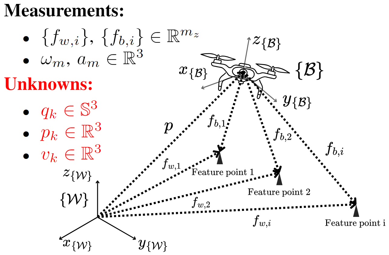
Figure 1: Navigation problem visualization in the 6 DoF.

IV QNUKF-based VIN Design

To develop the QNUKF, we will explore how the Conventional UKF (CUKF) [33] functions within the system. Next, we will modify each step to address the CUKF limitations. Stochastic filters, such as UKF models system parameters as RVs and aim to estimate the expected values of their distributions, which are then used as the estimates of the parameters. Let $X_{k}$ and $Z_{k}$ represent the RVs associated with the real values of $x_{k}$ and $z_{k}$, respectively. In this model, the expected values of the RVs are accounted as the real values. However, it should be noted that directly calculating these expected values is not feasible; instead, they are estimated. Let the estimated expected values of the probabilities $\mathbb{P}(X_{k-1}|Z_{k-1})$ and $\mathbb{P}(X_{k}|Z_{k-1})$ be $\hat{x}_{k-1|k-1}$ and $\hat{x}_{k|k-1}$, respectively, and the expected value of $\mathbb{P}(Z_{k})$ be $\hat{z}_{k|k-1}$.

IV-A Filter Initialization

Step 1. State and Covariance Initialization

At the QNUKF initialization, we establish the initial state estimate $\hat{x}_{0|0}$ and the covariance matrix $P_{0|0}$. While this step is standard in CUKF, managing quaternion-based navigation introduces unique challenges related to quaternion representation and covariance. A critical challenge arises from the fact that the covariance is computed based on differences from the mean. Thereby, straightforward quaternion subtraction is not feasible. To address this limitation, we employ the custom quaternion subtraction introduced in (17) and specifically designed for quaternion operations. Moreover, quaternions inherently possess three degrees of freedom while having four components, requiring adjustments to the covariance matrix to reflect the reduced dimensionality. Let the initial estimated state vector be defined as $\hat{x}_{0|0}=\left[\hat{x}_{0|0,q}^{\top},\hat{x}_{0|0,-}^{\top}\right]^{\top}\in\mathbb{R}^{m_{x}}$ (see (30)), where $\hat{x}_{0|0,q}\in\mathbb{S}^{3}$ and $\hat{x}_{0|0,-}\in\mathbb{R}^{m_{x}-4}$ represent the quaternion and non-quaternion components of $\hat{x}_{0|0}$, respectively, with $m_{x}$ being the number of rows in the state vector. The filter is initialized as:

$$\hat{x}_{0|0} =\left[\hat{x}_{0|0,q}^{\top},\hat{x}_{0|0,-}^{\top}\right]^{\top}\in\mathbb{R}^{m_{x}}$$ (38)

$$P_{0|0} =\text{diag}(P_{\hat{x}_{0|0,q}},P_{0|0,-})\in\mathbb{R}^{(m_{x}-1)\times(m_{x}-1)}$$ (39)

where $P_{0|0,q}\in\mathbb{R}^{3\times 3}$, $P_{0|0,-}\in\mathbb{R}^{(m_{x}-4)\times(m_{x}-4)}$, and $P_{0|0}$ represent the covariance matrices corresponding with the uncertainties of $\hat{x}_{0|0,q}$, $\hat{x}_{0|0,-}$, and $\hat{x}_{0|0}$, respectively.

IV-B Prediction

The prediction step involves estimating the state of the system at the next time step leveraging the system’s kinematics given the initial state (38) and covariance (39). At each $k$ time step, the process begins with augmenting the state vector with non-additive noise terms, a critical step that ensures the filter accounts for the uncertainty which these noise terms introduce. Subsequently, sigma points are generated from the augmented state vector and covariance matrix. These sigma points effectively represent the distribution $\mathbb{P}(X_{k-1}|Z_{k-1})$, capturing the state’s uncertainty at the previous time step given the previous observation, see (22). (20). The next phase involves computing the posterior sigma points by applying the state transition function to each sigma point, thereby representing the distribution $\mathbb{P}(X_{k}|X_{k-1})$ which is equivalent to $\mathbb{P}(X_{k}|Z_{k-1})$. This distribution reflects the predicted state’s uncertainty before the current observation is considered. The predicted state vector is then obtained as the weighted average of these posterior sigma points. This process is described in detail in this subsection.

Step 2. Augmentation

Prior to calculating the sigma points, the state vector and covariance matrix are augmented to incorporate non-additive process noise. This involves adding rows and columns to the state vector and covariance matrix to represent the process noise. The expected value of the noise terms, zero in this case, are augmented to the previous state estimate $\hat{x}_{k-1|k-1}$ to form the augmented state vector $\hat{x}_{k-1|k-1}^{a}$. Similarly, the last estimated state covariance matrix $P_{k-1|k-1}$ and the noise covariance matrix $C_{x,k}$ are augmented together to form the augmented state covariance matrix $P_{k-1|k-1}^{a}$. This is formulated as follows:

$$\hat{x}_{k-1|k-1}^{a} =\left[\hat{x}_{k-1|k-1}^{\top},0_{m_{n_{x}}\times 1}^{\top}\right]^{\top}\in\mathbb{R}^{m_{a}}$$ (40)

$$P_{k-1|k-1}^{a} =\text{diag}(P_{k-1|k-1},C_{x,k})\in\mathbb{R}^{(m_{a}-1)\times(m_{a}-1)}$$ (41)

The covariance matrix $C_{x,k}$ in (41) is defined by:

$$C_{x,k}=\text{diag}(C_{\omega,k},C_{a,k})\in\mathbb{R}^{m_{n_{x}}\times m_{n_{x}}}$$ (42)

Step 3. Sigma Points Calculation

Conventionally, sigma points are computed based on the augmented state estimate and covariance matrix. They serve as a representation for the distribution and uncertainty of $\mathbb{P}(x_{k-1|k-1}|z_{k-1})$. In other words, the greater the uncertainty of the last estimate reflected by a larger last estimated covariance, the more widespread the sigma points will be around the last estimated state. Reformulating (22) according to the CUKF algorithm, the sigma points, crucial for propagating the state through the system dynamics, are computed using the following equation:

$$\left\{\begin{aligned} \mathcal{X}_{k-1|k-1,0}^{a}&=\hat{x}_{k-1|k-1}^{a}\in\mathbb{R}^{m_{a}}\\ \mathcal{X}_{k-1|k-1,j}^{a}&=\hat{x}_{k-1|k-1}^{a}+\left(\sqrt{(m_{a}+\lambda)P_{k-1|k-1}^{a}}\right)_{j}\\ \mathcal{X}_{k-1|k-1,j+m_{a}}^{a}&=\hat{x}_{k-1|k-1}^{a}-\left(\sqrt{(m_{a}+\lambda)P_{k-1|k-1}^{a}}\right)_{j},\\ &\hskip 56.9055ptj=\{1,2,\ldots,2m_{a}\}\end{aligned}\right.$$ (43)

Challenges arise when using the sigma points calculation as described in (43) for quaternion-based navigation problems due to the differing mathematical spaces involved. For the sake of brevity, let us define $\delta\hat{x}_{k-1,j}^{a}:=\left(\sqrt{(m_{a}+\lambda)P_{k-1|k-1}^{a}}\right)_{j}\in\mathbb{R}^{m_{a}-1}$. It is possible to divide $\hat{x}_{k-1|k-1}^{a}$ and $\delta\hat{x}_{k-1,j}^{a}$ into their attitude and non-attitude parts: $\hat{x}_{k-1|k-1,q}\in\mathbb{S}^{3}$, $\delta\hat{x}_{k-1,j,r}^{a}\in\mathbb{R}^{3}$, and $\hat{x}_{k-1|k-1,-}^{a}\in\mathbb{R}^{m_{a}-4}$, $\delta\hat{x}_{k-1,j,-}^{a}\in\mathbb{R}^{m_{a}-4}$, as outlined below:

$$\left\{\begin{aligned} \hat{x}_{k-1|k-1}^{a}&=\left[(\hat{x}_{k-1|k-1,q}^{a})^{\top},(\hat{x}_{k-1|k-1,-}^{a})^{\top}\right]^{\top}\\ \delta\hat{x}_{k-1,j}^{a}&=\left[(\delta\hat{x}_{k-1,j,r}^{a})^{\top},(\delta\hat{x}_{k-1,j,-}^{a})^{\top}\right]^{\top}\end{aligned}\right.$$ (44)

From (44), given that $\delta\hat{x}_{k-1,j,r}^{a}$ is a rotation vector in $\mathbb{R}^{3}$ and $\hat{x}_{k-1|k-1,q}^{a}$ is a quaternion expression in $\mathbb{S}^{3}$, direct addition or subtraction is not feasible. To resolve this limitation, we employ the custom subtraction (16) and addition (15) operators, as previously defined. The operation map $\mathbb{S}^{3}\times\mathbb{R}^{3}\rightarrow\mathbb{S}^{3}$ effectively manages the interaction between quaternions and rotation vectors. Additionally, the quaternion-based navigation problem inherently possesses $m_{a}-1$ degrees of freedom due to the reduced dimensionality of the quaternion. To resolve this limitation, the propose QNUKF modifies $\delta\hat{x}_{k-1,j}^{a}$ as follows:

$$\delta\hat{x}_{k-1,j}^{a}:=\left(\sqrt{(m_{a}-1+\lambda)P_{k-1|k-1}^{a}}\right)_{j}\in\mathbb{R}^{m_{a}-1}$$ (45)

Overall, considering (44) and (45), the QNUKF utilizes the modified version of (43) as follows:

$$\left\{\begin{aligned} \mathcal{X}_{k-1|k-1,0}^{a}&=\hat{x}_{k-1|k-1}^{a}\in\mathbb{R}^{m_{a}}\\ \mathcal{X}_{k-1|k-1,j}^{a}&=\hat{x}_{k-1|k-1}^{a}\oplus\delta\hat{x}_{j}^{a}\\ &:=\begin{bmatrix}\hat{x}_{k-1|k-1,q}^{a}\oplus\delta\hat{x}_{k-1,j,r}^{a}\\ \hat{x}_{k-1|k-1,-}^{a}+\delta\hat{x}_{k-1,j,-}^{a}\end{bmatrix}\in\mathbb{R}^{m_{a}}\\ \mathcal{X}_{k-1|k-1,j+m_{a}}^{a}&=\hat{x}_{k-1|k-1}^{a}\ominus\delta\hat{x}_{j}^{a}\\ &:=\begin{bmatrix}\hat{x}_{k-1|k-1,q}^{a}\ominus\delta\hat{x}_{k-1,j,r}^{a}\\ \hat{x}_{k-1|k-1,-}^{a}-\delta\hat{x}_{k-1,j,-}^{a}\end{bmatrix}\in\mathbb{R}^{m_{a}},\\ &\hskip 42.67912ptj=\{1,2,\ldots,2(m_{a}-1)\}\end{aligned}\right.$$ (46)

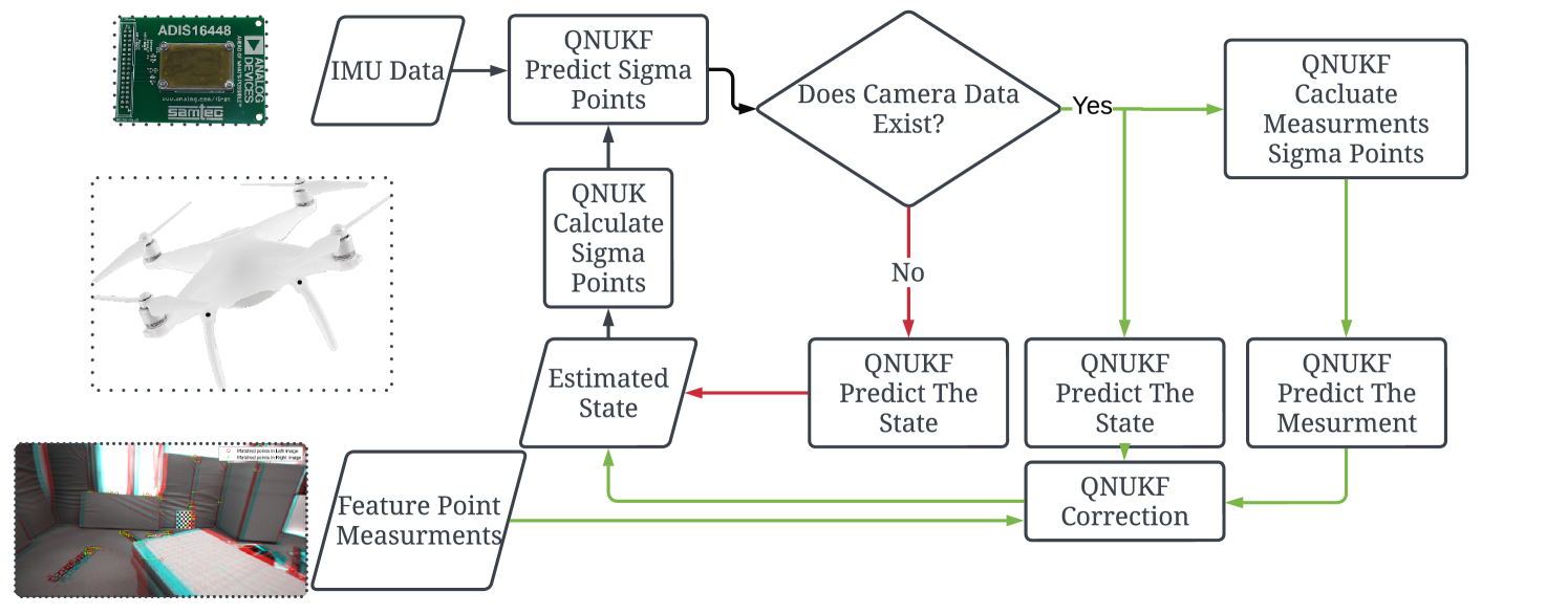
Figure 2: Schematic diagram of the proposed QNUKF. First, the sigma points based on the last estimated state vector and its covariance matrix are calculated. Using these sigma points and IMU measurements, the prediction step is performed. If camera data exists at that sample point, the correction (also known as update) step is performed. The state and covariance estimation at that time step is the result of the correction step if camera data exists, and the prediction step if it does not.

Step 4. Propagate Sigma Points

The sigma points $\{\mathcal{X}_{k-1|k-1,j}^{a}\}$ are propagated through the state transition function, as defined in (34), to calculate the propagated sigma points $\{\mathcal{X}_{k|k-1,j}\}$. These points represent the probability distribution $\mathbb{P}(X_{k}|X_{k-1})$, and are computed as follows:

$$\mathcal{X}_{k|k-1,j}= \operatorname{f}(\mathcal{X}_{k-1|k-1,j}^{a},u_{k-1})\in\mathbb{R}^{m_{x}}$$ (47)

for all $j=\{0,1,2,\ldots,2(m_{a}-1)\}$.

Step 5. Compute Predicted Mean and Covariance

The predicted mean $\hat{x}_{k|k-1}$ and covariance $P_{k|k-1}$ are conventionally computed using the predicted sigma points by reformulating (24) and (25) as:

$$\hat{x}_{k|k-1} =\sum_{j=0}^{2m_{a}}w_{j}^{m}\mathcal{X}_{k|k-1,j}\in\mathbb{R}^{m_{x}}$$ (48)

$$P_{k|k-1} =\sum_{j=0}^{2m_{a}}\left[w_{j}^{c}(\mathcal{X}_{k|k-1,j}-\hat{x}_{k|k-1})(\mathcal{X}_{k|k-1,j}-\hat{x}_{k|k-1})^{\top}\right]$$

$$\qquad+C_{w,k}\in\mathbb{R}^{(m_{x}-1)\times(m_{x}-1)}$$ (49)

where $w_{j}^{m}$ and $w_{j}^{c}\in\mathbb{R}$ represent the weights associated with the sigma points and are found by (23). Additionally, $C_{w,k}\in\mathbb{R}^{m_{x}-1}$ denotes the process noise covariance matrix, which is the covariance matrix of the noise vector $n_{w,k}$ as defined in (31). Note that the reduced dimensionality of $C_{w,k}$, similar to $P_{k|k-1}$ and $P_{0|0}$, is due to the covariance matrices of quaternion random variables being described by $3\times 3$ matrices, reflecting the three degrees of freedom inherent to quaternions. $C_{w,k}$ is defined as

$$C_{w,k}=\begin{bmatrix}0_{9\times 9}&0_{3\times 3}&0_{3\times 3}\\ 0_{9\times 9}&C_{b\omega,k}&0_{3\times 3}\\ 0_{9\times 9}&0_{3\times 3}&C_{ba,k}\end{bmatrix}\in\mathbb{R}^{(m_{x}-1)\times(m_{x}-1)}$$ (50)

To tailor (48), (49), and (23) for the quaternion-based navigation problem, the following modifications are necessary: (1) The QNUKF utilizes $m_{a}-1$ sigma points, therefore, all occurrences of $m_{a}$ in (48), (49), and (23) should be replaced with $m_{a}-1$; (2) The average of quaternion components of the sigma points in (48) should be computed using the quaternion weighted average method described in (18). This is necessary since the typical vector averaging method in (48) cannot be applied directly to quaternions; (3) The subtraction of quaternion components of the sigma point vector by the quaternion components of the estimated mean in (49) should utilize the custom subtraction method defined in (17). This operation maps $\mathbb{S}^{3}\times\mathbb{S}^{3}$ to $\mathbb{R}^{3}$, reflecting the fact that quaternions, which exist in $\mathbb{S}^{3}$ space, cannot be subtracted using conventional vector subtraction techniques.

To facilitate these operations, let us divide $\hat{x}_{k|k-1}$ and $\mathcal{X}_{k|k-1,j}$ to their quaternion ($\hat{x}_{k|k-1,q}\in\mathbb{S}^{3}$, $\mathcal{X}_{k|k-1,j,q}\in\mathbb{S}^{3}$) and non-quaternion ($\hat{x}_{k|k-1,-}\in\mathbb{R}^{n_{x}-4}$, $\mathcal{X}_{k|k-1,j,-}\in\mathbb{R}^{m_{x}-4}$) components. These divisions can be represented as follows:

$$\hat{x}_{k|k-1} =\begin{bmatrix}\hat{x}_{k|k-1,q}^{\top}&\hat{x}_{k|k-1,-}^{\top}\end{bmatrix}^{\top}\mathbb{R}^{m_{x}}$$ (51)

$$\mathcal{X}_{k|k-1,j} =\begin{bmatrix}\mathcal{X}_{k|k-1,q}^{\top}&\mathcal{X}_{k|k-1,-}^{\top}\end{bmatrix}^{\top}\in\mathbb{R}^{m_{x}}$$ (52)

Consequently, equations (48), (49), and (23) can be reformulated to accommodate these quaternion-specific processes, utilizing the divisions formulated in (51) and (52) as follows:

$$\hat{x}_{k|k-1} =\begin{bmatrix}\operatorname{QWA}(\{\mathcal{X}_{k|k-1,j,q}\},\{w_{j}^{m}\})\\ {\displaystyle\sum_{j=0}^{2(m_{a}-1)}w_{j}^{m}\mathcal{X}_{k|k-1,j,-}}\end{bmatrix}\in\mathbb{R}^{m_{x}}$$ (53)

$$P_{k|k-1} =\sum_{j=0}^{2(m_{a}-1)}\left[w_{j}^{c}(\mathcal{X}_{k|k-1,j}\ominus\hat{x}_{k|k-1})(\mathcal{X}_{k|k-1,j}\ominus\hat{x}_{k|k-1})^{\top}\right]$$

$$\qquad+C_{w,k}\in\mathbb{R}^{(m_{x}-1)\times(m_{x}-1)}$$ (54)

and

$$\left\{\begin{aligned} w_{0}^{m}&=\frac{\lambda}{\lambda+(m_{a}-1)}\in\mathbb{R}\\ w_{0}^{c}&=\frac{\lambda}{\lambda+(m_{a}-1)}+1-\alpha^{2}+\beta\in\mathbb{R}\\ w_{j}^{m}&=w_{j}^{c}=\frac{1}{2((m_{a}-1)+\lambda)}\in\mathbb{R}\\ &\hskip 56.9055ptj=\{1,\ldots,2(m_{a}-1)\}\end{aligned}\right.$$ (55)

where

$$\mathcal{X}_{k|k-1,j}\ominus\hat{x}_{k|k-1} =\begin{bmatrix}\mathcal{X}_{k|k-1,j,q}\ominus\hat{x}_{k|k-1,q}\\ \mathcal{X}_{k|k-1,j,-}-\hat{x}_{k|k-1,-}\end{bmatrix}\in\mathbb{R}^{m_{x}-1}$$ (56)

IV-C Update

In the update step, the propagated sigma points are first processed through the measurement function to generate the measurement sigma points, which represent $\mathbb{P}(Z_{k}|X_{k})$. Subsequently, utilizing $\mathbb{P}(X_{k-1}|Z_{k-1})$, $\mathbb{P}(X_{k}|X_{k-1})$, and $\mathbb{P}(Z_{k}|X_{k})$, the conditional probability $\mathbb{P}(X_{k}|Z_{k})$ is estimated. The expected value derived from $\mathbb{P}(X_{k}|Z_{k})$ will serve as the state estimate for the $k$th step.

Step 6. Predict Measurement and Calculate Covariance

In this step, each propagated sigma point $\mathcal{X}_{k|k-1,j}$, as found in (47), is processed through the measurement function defined in (37) to compute the $j$th predicted sigma point $\mathcal{Z}_{k|k-1,j}$. The set $\{\mathcal{Z}_{k|k-1,j}\}$ represent the probability distribution $\mathbb{P}(Z_{k}|X_{k})$. For all $j=\{0,1,\ldots,2(m_{a}-1)\}$, the computation for each sigma point is given by:

$$\mathcal{Z}_{k|k-1,j} =h(\mathcal{X}_{k|k-1,j},f_{w})\in\mathbb{R}^{m_{z}}$$ (57)

The expected value of $\mathbb{P}(Z_{k}|X_{k})$ is the maximum likelihood estimate of the measurement vector. This estimate $\hat{z}_{k|k-1}$ is calculated according to (58). Additionally, the estimated measurement covariance matrix $P_{z_{k},z_{k}}\in\mathbb{R}^{m_{z}\times m_{z}}$ and the state-measurement covariance matrix $P_{x_{k},z_{k}}\in\mathbb{R}^{(m_{x}-1)\times m_{z}}$ are computed using the following equations:

$$\hat{z}_{k|k-1} =\sum_{j=0}^{2(m_{a}-1)}w_{j}^{m}\mathcal{Z}_{k|k-1,j}$$ (58)

$$P_{z_{k},z_{k}} =\sum_{j=0}^{2(m_{a}-1)}w_{j}^{c}[\mathcal{Z}_{k|k-1,j}-\hat{z}_{k|k-1}][\mathcal{Z}_{k|k-1,j}-\hat{z}_{k|k-1}]^{\top}$$

$$\hskip 42.67912pt+C_{f}$$ (59)

$$P_{x_{k},z_{k}} =\sum_{j=0}^{2(m_{a}-1)}w_{j}^{c}[\mathcal{X}_{k|k-1,j}\ominus\hat{x}_{k|k-1}][\mathcal{Z}_{k|k-1,j}-\hat{z}_{k|k-1}]^{\top}$$ (60)

Note that the subtraction operator $\ominus$ in (60) denotes state difference operator and follows (56). Now, the joint distribution of $(X_{k},Z_{k})$ is estimated as follows:

$$\begin{pmatrix}X_{k}\\[5.0pt] Z_{k}\end{pmatrix}\sim\mathcal{N}\left(\begin{pmatrix}\hat{x}_{k|k-1}\\[5.0pt] \hat{z}_{k|k-1}\end{pmatrix},\begin{pmatrix}P_{k|k-1}&P_{x_{k},z_{k}}\\[5.0pt] P_{x_{k},z_{k}}^{\top}&P_{z_{k},z_{k}}\end{pmatrix}\right)$$ (61)

These covariance calculations are necessary to estimate the probability distribution $\mathbb{P}(X_{k}|Z_{k})$ in the next step.

Step 7. Update State Estimate

In view of (61) to (19), let us reformulate (20) to find the mean and covariance estimate of the $\mathbb{P}(X_{k}|Z_{k})$ distribution. It is worth noting that the estimated mean is the estimated state vector at this time step. This is achieved by computing the Kalman gain $K_{k}\in\mathbb{R}^{(m_{x}-1)\times m_{z}}$ given the matrices found in (59) and (60).

$$K_{k}=P_{x_{k},z_{k}}P_{z_{k},z_{k}}^{\top}\in\mathbb{R}^{(m_{x}-1)\times m_{z}}$$ (62)

To find the updated covariance estimate of the state distribution $P_{k|k}$ in the QNUKF, the conventional formula provided in (63) is utilized:

$$P_{k|k}=P_{k|k-1}-K_{k}P_{z_{k},z_{k}}K_{k}^{\top}$$ (63)

However, computing the updated estimated state vector $\hat{x}_{k|k}$ requires careful consideration. Define the correction vector $\delta\hat{x}_{k|k-1}$ as:

$$\delta\hat{x}_{k|k-1}:=K_{k}(z_{k}-\hat{z}_{k|k-1})\in\mathbb{R}^{m_{x}-1}$$ (64)

Recall that $z_{k}$ refers to camera feature measurements in $\{\mathcal{B}\}$. Conventionally, the correction vector calculated in (64), is added to the predicted state vector from (53) to update the state. However, for a quaternion-based navigation problem, the dimensions of $\delta\hat{x}_{k|k-1}$ and $\hat{x}_{k|k-1}$ do not match, with the former being $m_{x}-1$ and the latter $m_{x}$. To address this, let us divide $\delta\hat{x}_{k|k-1}$ into its attitude ($\delta\hat{x}_{k|k-1,r}\in\mathbb{R}^{3}$) and non-attitude ($\delta\hat{x}_{k|k-1,-}\in\mathbb{R}^{m_{\star}-4}$) components:

$$\delta\hat{x}_{k|k-1}=\begin{bmatrix}\delta\hat{x}_{k|k-1,r}^{\top}&\delta\hat{x}_{k|k-1,-}^{\top}\end{bmatrix}^{\top}$$ (65)

From (65) with (51), we observe that the non-quaternion components of $\hat{x}_{k|k-1}$ and $\delta\hat{x}_{k|k-1}$ are dimensionally consistent and can be combined using the conventional addition operator. However, the orientation components of $\hat{x}_{k|k-1}$ and $\delta\hat{x}_{k|k-1}$ do not match dimensionally. The former is represented by a quaternion within the $\mathbb{S}^{3}$ space, while the latter is a rotation vector in the three-dimensional Euclidean space $\mathbb{R}^{3}$. To add the orientation parts of the predicted state and correction vectors, the custom summation operator $\mathbb{S}^{3}\times\mathbb{R}^{3}\rightarrow\mathbb{S}^{3}$ described in (15) should be used as follows

$$\hat{x}_{k|k}=\hat{x}_{k|k-1}\oplus\delta\hat{x}_{k|k-1}$$ (66)

where

$$\hat{x}_{k|k-1}\oplus\delta\hat{x}_{k|k-1}=\begin{bmatrix}\hat{x}_{k|k-1,q}\oplus\delta\hat{x}_{k|k-1,r}\\ \hat{x}_{k|k-1,-}+\delta\hat{x}_{k|k-1,-}\end{bmatrix}$$ (67)

Step 8. Iterate

Go back to Step 2. and iterate from $k\rightarrow k+1$.

The proposed QNUKF algorithm is visually depicted in Fig. 2. The implementation steps of QNUKF algorithm is summarized and outlined in Algorithm 1.

Remark 1.

The time complexities of the vanilla EKF and UKF algorithms are $O(m_{x}^{3})$ and $O(m_{a}^{3})$, respectively [39]. For navigation tasks, these complexities reduce to $O((m_{x}-1)^{3})$ and $O((m_{a}-1)^{3})$, respectively, due to the reduced dimensionality of the quaternion in the state vector. The custom operations proposed in QNUKF, such as the one used in (67), all have complexities less than $O((m_{a}-1))$ and occur only once for each sigma point. Therefore, QNUKF retains the same overall complexity as any UKF, which is $O((m_{a}-1)^{3})$. The difference between $m_{a}$ and $m_{x}$ arises because UKF can capture non-additive noise terms by augmenting them into the state vector, whereas EKF linearizes them into an additive form.

Algorithm 1 Quaternion Navigation Unscented Kalman Filter

Initialization:

1. Set $\hat{x}_{0|0}\in\mathbb{R}^{m_{x}-4}$, see (30), and $P_{0|0}\in\mathbb{R}^{(m_{x}-1)\times(m_{x}-1)}$.

2. Set $k=0$ and select the filter design parameters $\lambda$, $\alpha$, $\beta\in\mathbb{R}$, along with the noise covariance matrices $C_{a,k}$, $C_{\omega,k}$, $C_{ba,k}$, $C_{b\omega,k}\in\mathbb{R}^{3\times 3}$, and the noise variance $c_{f}\in\mathbb{R}$.

3. Calculate $C_{x,k}$, $C_{w,k}$, and $C_{f}$ as expressed in (42), (50), and (68), respectively.

while IMU data exists

1. /* Prediction */

2. $\begin{cases}\hat{x}_{k-1|k-1}^{a}&=\left[\hat{x}_{k-1|k-1}^{\top},0_{6\times 1}^{\top}\right]^{\top}\in\mathbb{R}^{(m_{a}-1)\times 1}\\ P_{k-1|k-1}^{a}&=\begin{bmatrix}P_{k-1|k-1}&0_{(m_{x}-1)\times m_{n_{x}}}\\ 0_{m_{n_{x}}\times(m_{x}-1)}&C_{x,k}\end{bmatrix}\end{cases}$

3. $\mathcal{X}_{k-1|k-1,0}^{a}=\hat{x}_{k-1|k-1}^{a}$

4. for $j=\{1,2\ldots,(m_{a}-1)\}$

5. $\qquad\delta\hat{x}_{k-1,j}^{a}:=\left(\sqrt{(m_{a}-1+\lambda)P_{k-1|k-1}^{a}}\right)_{j}$, see (45)

6. $\qquad\mathcal{X}_{k-1|k-1,j}^{a}=\hat{x}_{k-1|k-1}^{a}\oplus\delta\hat{x}_{j}^{a}$, see (46)

7. $\qquad\mathcal{X}_{k-1|k-1,j+m_{a}}^{a}=\hat{x}_{k-1|k-1}^{a}\ominus\delta\hat{x}_{j}^{a}$, see (46)

8. end for

9. for $j=\{1,2\ldots,(m_{a}-1)\}$

10. $\qquad\qquad\mathcal{X}_{k|k-1,j}=\operatorname{f}(\mathcal{X}_{k-1|k-1,j}^{a},u_{k-1})$

11. end for, see (47)

12. $\hat{x}_{k|k-1}=\begin{bmatrix}\operatorname{QWA}(\{\mathcal{X}_{k|k-1,j,q}\},\{w_{j}^{m}\})\\ {\displaystyle\sum_{j=0}^{2(m_{a}-1)}w_{j}^{m}\mathcal{X}_{k|k-1,j,-}}\end{bmatrix}$, see (53)

13. $P_{k|k-1}=\sum_{j=0}^{2(m_{a}-1)}[w_{j}^{c}(\mathcal{X}_{k|k-1,j}\ominus\hat{x}_{k|k-1})(\mathcal{X}_{k|k-1,j}\ominus\hat{x}_{k|k-1})^{\top}]+C_{w,k}$, see (54)

14. /* Update step */

15. for $j=\{0,1,2\ldots,(m_{a}-1)\}$

16. $\qquad\mathcal{Z}_{k|k-1,j}=h(\mathcal{X}_{k|k-1,j}^{a},f_{w})$

17. end for, see (57)

18. $\hat{z}_{k|k-1}=\sum_{j=0}^{2(m_{a}-1)}w_{j}^{m}\mathcal{Z}_{k|k-1,j}$, see (58)

19. $P_{z_{k},z_{k}}=\sum_{j=0}^{2(m_{a}-1)}w_{j}^{c}[\mathcal{Z}_{k|k-1,j}-\hat{z}_{k|k-1}][\mathcal{Z}_{k|k-1,j}-\hat{z}_{k|k-1}]^{\top}+C_{f}$, see (59)

20. $P_{x_{k},z_{k}}=\sum_{j=0}^{2(m_{a}-1)}w_{j}^{c}[\mathcal{X}_{k|k-1,j}\ominus\hat{x}_{k|k-1}][\mathcal{Z}_{k|k-1,j}-\hat{z}_{k|k-1}]^{\top}$, see (60)

21. $\begin{cases}K_{k}&=P_{x_{k},z_{k}}P_{z_{k},z_{k}}^{\top}\\ \delta\hat{x}_{k|k-1}&=K(z_{k}-\hat{z}_{k|k-1})\\ \hat{x}_{k|k}&=\hat{x}_{k|k-1}\oplus\delta\hat{x}_{k|k-1}\\ P_{k|k}&=P_{k|k-1}-K_{k}P_{z_{k},z_{k}}K_{k}^{\top}\end{cases}$, see (67)

22. $k=k+1$

end while

V Implementation and Results

To evaluate the effectiveness of the proposed QNUKF, the algorithm is tested using the real-world EuRoC dataset of drone flight in 6 DoF [40]. For video of the experiment, visit the following link. This dataset features an Asctec Firefly hex-rotor Micro Aerial Vehicle (MAV) flown in a static indoor environment, from which IMU, stereo images, and ground truth data were collected. The stereo images are two simultaneous monochrome images obtained via an Aptina MT9V034 global shutter sensor with a 20 Hertz frequency. Linear acceleration and angular velocity of the MAV were measured by an ADIS16448 sensor with a 200 Hertz frequency. Note that the data sampling frequency of the camera and IMU are different. Consequently, the measurement data does not necessarily exist at each IMU data sample point. To incorporate this, the system only performs the update step when image data is retrieved, and sets $\hat{x}_{k|k}$ equal to the predicted estimated state vector $\hat{x}_{k|k-1}$ when image data is unavailable.

V-A The Proposed QNUKF Output Performance

The feature point count $m_{f}$ is not constant at each measurement step, to compensate for this, we set the measurement noise covariance to:

$$C_{f}=c_{f}^{2}I_{m_{f}}$$ (68)

where $m_{f}$ is based on the number of feature points at each measurement step and $c_{f}$ is a scaler tuned beforehand. To ensure the covariance matrices remain symmetric and avoid numerical issues, for any $P\in\mathbb{R}^{m_{P}\times m_{P}}$, the $\operatorname{Symmetrize}$ function is defined as $\operatorname{Symmetrize}:\mathbb{R}^{m_{P}\times m_{P}}\rightarrow\mathbb{R}^{m_{P}\times m_{P}}$:

$$\operatorname{Symmetrize}(P):=\frac{P+P^{\top}}{2}\in\mathbb{R}^{m_{P}\times m_{P}}.$$ (69)

This function is applied to all single-variable covariance matrices after they are calculated according to the QNUKF. The filter parameters are configured as follows: $\lambda=3-(m_{a}-1)$, $\alpha=10^{-4}$, and $\beta=2$. The IMU bias noise covariances are determined by the standard deviations (std) of the bias white noise terms, set to $0.01\%$ of their average values to account for the slow random walk relative to the IMU sampling rate. These values are configured as: $C_{ba,k}=10^{-8}\text{diag}(0.0022^{2},0.0208^{2},0.0758^{2})$ $(m/s^{2})^{2}$ and $C_{b\omega,k}=10^{-8}\text{diag}(0.0147^{2},0.1051^{2},0.0930^{2})$ $(rad/s)^{2}$. The std of the additive white noise terms are set to $1\%$ of the measured vectors (i.e., linear acceleration and angular velocity) such that the covariance matrices are $C_{\omega,k}=10^{-4}\text{diag}(0.1356^{2},0.0386^{2},0.0242^{2})$ $(m/s^{2})^{2}$ and $C_{a,k}=10^{-4}\text{diag}(9.2501^{2},0.0293^{2},-3.3677^{2})$ $(rad/s)^{2}$. The measurement noise std is calculated using the measurement vectors from the V1_01_hard dataset [40], recorded in the same room as the validation V1_02_medium dataset [40], but with different drone paths and complexity speeds. Its value is found as $c_{f}=0.099538$ m. For each set of stereo images obtained, feature points are identified using the Kanade-Lucas-Tomasi (KLT) algorithm [41]. An example of the feature match results from this operation is depicted in Fig. 3.

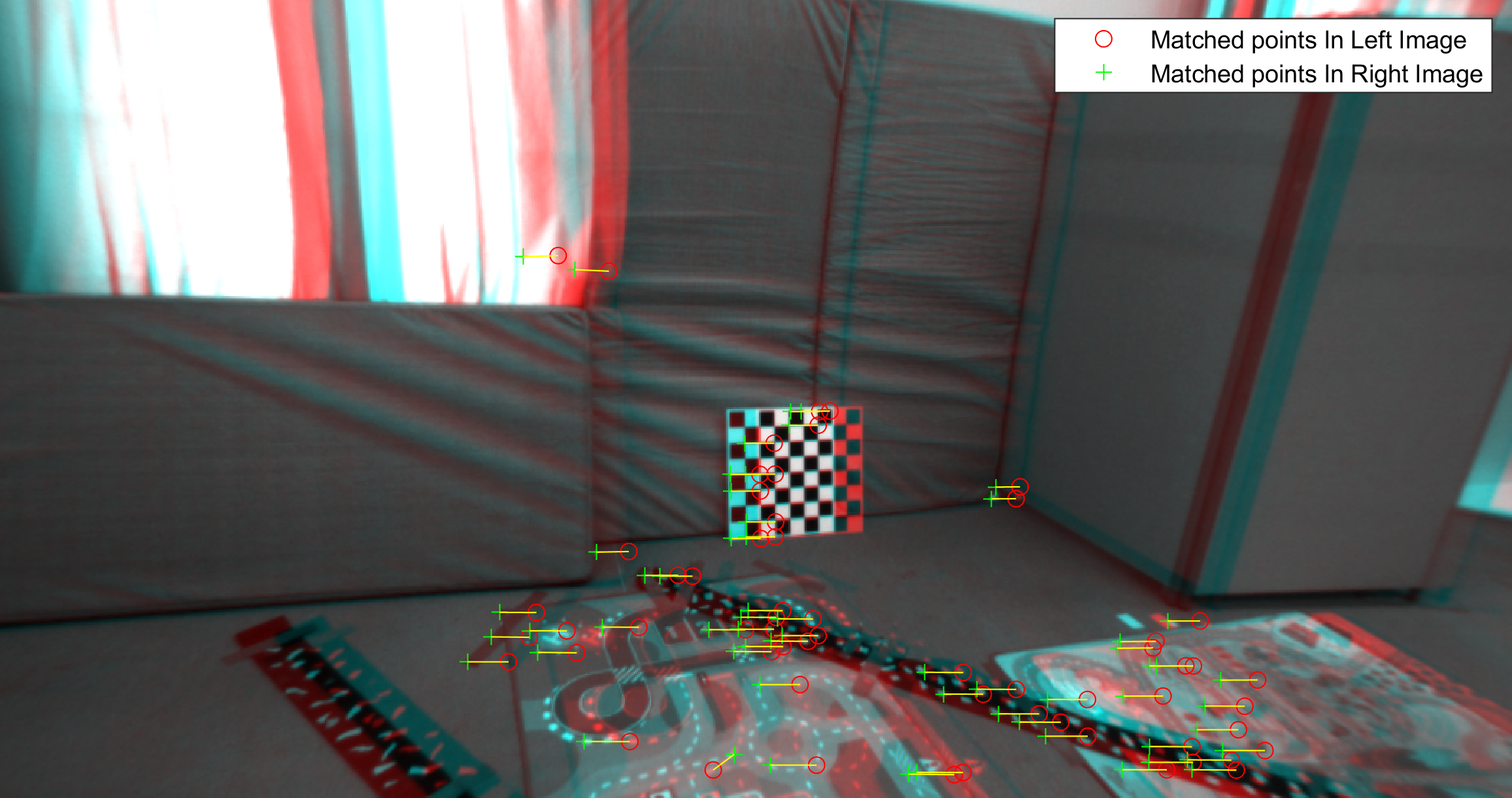
Figure 3: Matched feature points from the left and right views of the EuRoC dataset [40].

Using triangulation [42], the 2D matched points are projected to the 3D space, representing the feature points in $\{\mathcal{W}\}$. Using the $\mathbb{S}^{3}\times\mathbb{S}^{3}\rightarrow\mathbb{R}^{3}$ subtraction operator defined in (17), let us define the orientation estimation error $r_{e,k}$ as:

$$r_{e,k}:=q_{k}\ominus\hat{q}_{k}$$ (70)

where $r_{e,k}=\begin{bmatrix}r_{e1,k}&r_{e2,k}&r_{e3,k}\end{bmatrix}^{\top}\in\mathbb{R}^{3}$, with each component $r_{ei,k}\in\mathbb{R}$ representing a dimension of the error vector. Similarly, let us define the position and linear velocity estimation errors at the $k$th time step, represented by $p_{e,k}$ and $v_{e,k}$, respectively, as:

$$p_{e,k} :=p_{k}-\hat{p}_{k}$$ (71)

$$v_{e,k} :=v_{k}-\hat{v}_{k}$$ (72)

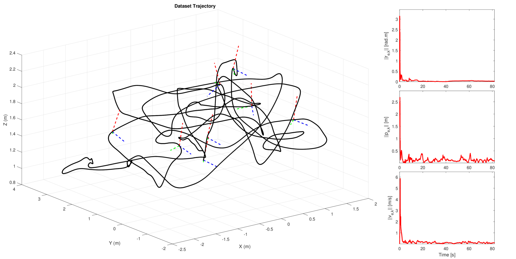
Figure 4: Validation results of the proposed QNUKF using the EuRoC V1_02_medium dataset [40]. On the left, the navigation trajectory of the drone moving in 3D space is shown with a solid black line, and the drone orientation with respect to $x$, $y$, and $z$ axes is represented by red, green, and blue dashed lines, respectively. On the right, the magnitudes of the orientation error vector $||r_{e,k}||$, position error vector $||p_{e,k}||$, and linear velocity error vector $||v_{e,k}||$ are plotted over time in solid red lines.

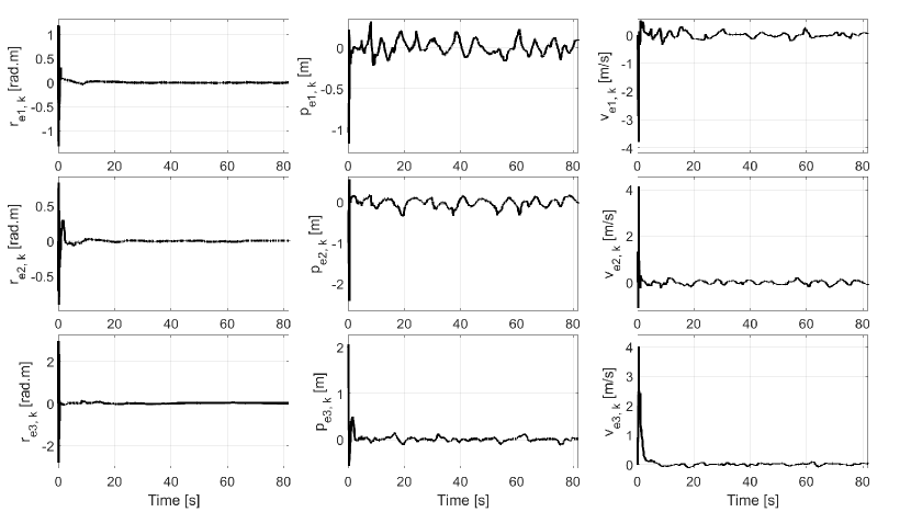
Figure 5: Estimation errors in rotation vector (left), position (middle), and linear velocity (right) components, from top to bottom of the proposed QNUKF.

where $p_{e,k}=\begin{bmatrix}p_{e1,k}&p_{e2,k}&p_{e3,k}\end{bmatrix}^{\top}\in\mathbb{R}^{3}$ and $v_{e,k}=\begin{bmatrix}v_{e1,k}&v_{e2,k}&v_{e3,k}\end{bmatrix}^{\top}\in\mathbb{R}^{3}$. The robustness and effectiveness of the proposed QNUKF have been confirmed through experimental results on the EuRoC V1_02_medium dataset [40] as depicted in Fig. 4 and with the initial estimates for the state vector and covariance matrix being detailed as follows: $\hat{x}_{0:0}=[$$0.1619$, $0.7900$, $-0.2053$, $0.5545$, $0.6153$, $2.0967$, $0.7711$, $0$, $0$, $0$, $-0.0022$, $0.0208$, $0.0758$, $-0.0147$, $0.1051$, $0.0930$$]^{\top}$ and $P_{0|0}=\text{diag}(80I_{3},10I_{3},70I_{3},10I_{6})$. On the left side of Fig. 4, the trajectory and orientation of the drone during the experiment are depicted. On the right side, the magnitudes of the orientation, position, and linear velocity error vectors are plotted over time. The results demonstrate that all errors converge to near-zero values and recover from initial large errors rapidly, indicating excellent performance. To examine the filter’s performance in detail, each component of the estimation error is plotted against time. These plots are displayed in Fig. 5, showing excellent performance in tracking each component of orientation, position, and linear velocity.

V-B Comparison with State-of-the-art Literature

For video of the comparison, visit the following link. To evaluate the efficacy of the proposed filter, we compared its performance with the vanilla Extended Kalman Filter (EKF), the standard tool in non-linear estimation problems as well as the Multi-State Constraint Kalman Filter (MSCKF) [43], which addresses the observability issues of the EKF caused by linearization. Both models were implemented to operate with the same state vectors (as defined in (30)), state transition function (as defined in (34)), and measurement function (as defined in (37)). Additionally, their noise covariance parameters, as well as initial state and covariance matrices, were set to identical values in each experiment for all the filters to ensure a fair comparison. In light of (70), (71), and (72), let us define the estimation error at time step $k$ denoted by $e_{k}$ as:

$$e_{k}=||r_{e,k}||+||p_{e,k}||+||v_{e,k}||\in\mathbb{R}$$ (73)

Using (73), the Root Mean Square Error (RMSE) is calculated as:

$$\text{RMSE}=\sqrt{\frac{1}{m_{k}}\sum_{k=1}^{m_{k}}e_{k}^{2}}$$

where $m_{k}$ is the total number of time steps. The steady state root mean square error (SSRMSE) is defined similarly to RMSE but calculated over the last 20 seconds of the experiment. Table II compares the performance of the EKF, MSCKF, and QNUKF across three different EuRoC [40] datasets using RMSE and SSRMSE as metrics. Experiments 1, 2, and 3 correspond to the V1_02_medium, V1_03_difficult, and V2_01_easy datasets, respectively, with the best RMSE and SSRMSE values in each experiment. The proposed QNUKF algorithm consistently outperformed the other filters across all experiments and metrics. While the MSCKF showed better performance than the EKF, it lacked consistency, with RMSE values ranging from $0.866786$ to $1.454449$. In contrast, the QNUKF maintained a more stable performance, with RMSE values tightly clustered between $0.265037$ and $0.331952$.

TABLE II: Performance Comparison of QNUKF (proposed) vs EKF and MSCKF (literature) on EuRoC Datasets.

Filter	Metric	Experiment 1	Experiment 2	Experiment 3
EKF	RMSE	$0.952955$	$0.831777$	$1.411102$
	SSRMSE	$0.123161$	$0.160883$	$0.263435$
MSCKF	RMSE	$0.866786$	$1.175951$	$1.454449$
	SSRMSE	$0.074154$	$0.062882$	$0.075329$
QNUKF	RMSE	$0.331952$	$0.275067$	$0.265037$
	SSRMSE	$0.059464$	$0.051633$	$0.060865$

Let us examine the orientation, position, and linear velocity estimation error trajectories for all the filters in Experiment 2 as a case study. As depicted in Fig. 6, the QNUKF outperformed the other filters across all estimation errors. The EKF exhibited a slow response in correcting the initial error, while the MSCKF corrected course more quickly but initially overshot compared to the EKF. In contrast, the QNUKF responded rapidly and maintained smaller steady-state errors when compared with EKF and MSCKF.

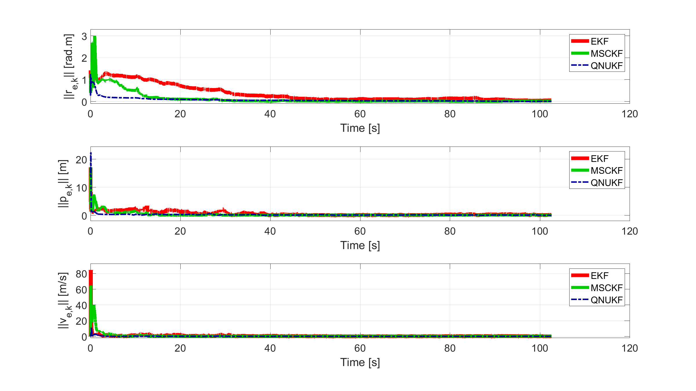
Figure 6: Estimation errors in orientation (top), position (middle), and linear velocity (bottom) for the EKF (red thick solid line), MSCKF (green solid line), and proposed QNUKF (blue dashed line).

VI Conclusion

In this paper, we investigated the orientation, position, and linear velocity estimation problem for a rigid-body navigating in three-dimensional space with six degrees-of-freedom. A robust Unscented Kalman Filter (UKF) is developed, incorporating quaternion space, ensuring computational efficiency at low sampling rates, handling kinematic nonlinearities effectively, and avoiding orientation singularities, such as those common in Euler angle-based filters. The proposed Quaternion-based Navigation Unscented Kalman Filter (QNUKF) relies on onboard Visual-Inertial Navigation (VIN) sensor fusion of data obtained by a stereo camera (feature observations and measurements) and a 6-axis Inertial Measurement Unit (IMU) (angular velocity and linear acceleration). The performance of the proposed algorithm was validated using real-world dataset of a drone flight travelling in GPS-denied regions where stereo camera images and IMU data were collected at low sampling rate. The results demonstrated that the algorithm consistently achieved excellent performance, with orientation, position, and linear velocity estimation errors quickly converging to near-zero values, despite significant initial errors and the use of low-cost sensors with high uncertainty. The proposed algorithm consistently outperformed both baseline and state-of-the-art filters, as demonstrated by the three experiments conducted in two different rooms.

As the next step, we will investigate the effectiveness of adaptive noise covariance tuning on QNUKF to mitigate this issue. Additionally, reworking QNUKF to address simultaneous localization and mapping (SLAM) for UAVs is a consideration for future work, as it represents a natural progression from navigation.

References

- [1] H. A. Hashim, “GPS-denied navigation: Attitude, position, linear velocity, and gravity estimation with nonlinear stochastic observer,” in 2021 American Control Conference (ACC). IEEE, 2021, pp. 1149–1154.
- [2] Y. Xu, Y. S. Shmaliy, S. Bi, X. Chen, and Y. Zhuang, “Extended kalman/ufir filters for uwb-based indoor robot localization under time-varying colored measurement noise,” IEEE Internet of Things Journal, vol. 10, no. 17, pp. 15 632–15 641, 2023.
- [3] H. A. Hashim, A. E. Eltoukhy, and A. Odry, “Observer-based controller for VTOL-UAVs tracking using direct vision-aided inertial navigation measurements,” ISA transactions, vol. 137, pp. 133–143, 2023.
- [4] Q. Wang, H. Luo, H. Xiong, A. Men, F. Zhao, M. Xia, and C. Ou, “Pedestrian dead reckoning based on walking pattern recognition and online magnetic fingerprint trajectory calibration,” IEEE Internet of Things Journal, vol. 8, no. 3, pp. 2011–2026, 2020.
- [5] H. A. Hashim, M. Abouheaf, and M. A. Abido, “Geometric stochastic filter with guaranteed performance for autonomous navigation based on IMU and feature sensor fusion,” Control Engineering Practice, vol. 116, p. 104926, 2021.
- [6] O. Asraf, F. Shama, and I. Klein, “Pdrnet: A deep-learning pedestrian dead reckoning framework,” IEEE Sensors Journal, vol. 22, no. 6, pp. 4932–4939, 2021.
- [7] C. Jiang, Y. Chen, C. Chen, J. Jia, H. Sun, T. Wang, and J. Hyyppa, “Implementation and performance analysis of the pdr/gnss integration on a smartphone,” GPS Solutions, vol. 26, no. 3, p. 81, 2022.
- [8] H. A. Hashim, L. J. Brown, and K. McIsaac, “Nonlinear stochastic attitude filters on the special orthogonal group 3: Ito and stratonovich,” IEEE Transactions on Systems, Man, and Cybernetics: Systems, vol. 49, no. 9, pp. 1853–1865, 2018.
- [9] S. Carletta, P. Teofilatto, and M. S. Farissi, “A magnetometer-only attitude determination strategy for small satellites: Design of the algorithm and hardware-in-the-loop testing,” Aerospace, vol. 7, no. 1, p. 3, 2020.
- [10] H. A. Hashim, “Systematic convergence of nonlinear stochastic estimators on the special orthogonal group SO (3),” International Journal of Robust and Nonlinear Control, vol. 30, no. 10, pp. 3848–3870, 2020.
- [11] D. Scaramuzza and et al., “Vision-controlled micro flying robots: from system design to autonomous navigation and mapping in GPS-denied environments,” IEEE Robotics & Automation Magazine, vol. 21, no. 3, pp. 26–40, 2014.
- [12] H.-P. Tan, R. Diamant, W. K. Seah, and M. Waldmeyer, “A survey of techniques and challenges in underwater localization,” Ocean Engineering, vol. 38, no. 14-15, pp. 1663–1676, 2011.
- [13] G. P. Roston and E. P. Krotkov, Dead Reckoning Navigation For Walking Robots. Department of Computer Science, Carnegie-Mellon University, 1991.
- [14] H. Zhou, Y. Zhao, X. Xiong, Y. Lou, and S. Kamal, “IMU dead-reckoning localization with rnn-iekf algorithm,” in 2022 IEEE/RSJ International Conference on Intelligent Robots and Systems (IROS). IEEE, 2022, pp. 11 382–11 387.
- [15] H. A. Hashim, A. E. Eltoukhy, and K. G. Vamvoudakis, “UWB ranging and IMU data fusion: Overview and nonlinear stochastic filter for inertial navigation,” IEEE Transactions on Intelligent Transportation Systems, 2023.
- [16] S. Zheng, Z. Li, Y. Liu, H. Zhang, and X. Zou, “An optimization-based UWB-IMU fusion framework for UGV,” IEEE Sensors Journal, vol. 22, no. 5, pp. 4369–4377, 2022.
- [17] H. H. Helgesen and et al., “Inertial navigation aided by ultra-wideband ranging for ship docking and harbor maneuvering,” IEEE Journal of Oceanic Engineering, vol. 48, no. 1, pp. 27–42, 2022.
- [18] W. You, F. Li, L. Liao, and M. Huang, “Data fusion of UWB and IMU based on unscented kalman filter for indoor localization of quadrotor uav,” IEEE Access, vol. 8, pp. 64 971–64 981, 2020.
- [19] P. J. Besl and N. D. McKay, “Method for registration of 3-d shapes,” in Sensor fusion IV: control paradigms and data structures, vol. 1611. Spie, 1992, pp. 586–606.
- [20] A. Myronenko and X. Song, “Point set registration: Coherent point drift,” IEEE transactions on pattern analysis and machine intelligence, vol. 32, no. 12, pp. 2262–2275, 2010.
- [21] H. A. Hashim, “A geometric nonlinear stochastic filter for simultaneous localization and mapping,” Aerospace Science and Technology, vol. 111, p. 106569, 2021.
- [22] Z. Bai, H. Xu, Q. Ding, and X. Zhang, “Side-scan sonar image classification with zero-shot and style transfer,” IEEE Transactions on Instrumentation and Measurement, 2024.
- [23] J. A. Christian and S. Cryan, “A survey of lidar technology and its use in spacecraft relative navigation,” in AIAA Guidance, Navigation, and Control (GNC) Conference, 2013, p. 4641.
- [24] Y. Wei and Y. Xi, “Optimization of 3-d pose measurement method based on binocular vision,” IEEE Transactions on Instrumentation and Measurement, vol. 71, pp. 1–12, 2023.
- [25] D. Murray and J. J. Little, “Using real-time stereo vision for mobile robot navigation,” autonomous robots, vol. 8, pp. 161–171, 2000.
- [26] T. Huntsberger, H. Aghazarian, A. Howard, and D. C. Trotz, “Stereo vision–based navigation for autonomous surface vessels,” Journal of Field Robotics, vol. 28, no. 1, pp. 3–18, 2011.
- [27] J. Kim and S. Sukkarieh, “Real-time implementation of airborne inertial-slam,” Robotics and Autonomous Systems, vol. 55, no. 1, pp. 62–71, 2007.
- [28] J. Huang, S. Wen, W. Liang, and W. Guan, “Vwr-slam: Tightly coupled slam system based on visible light positioning landmark, wheel odometer, and rgb-d camera,” IEEE Transactions on Instrumentation and Measurement, vol. 72, pp. 1–12, 2022.
- [29] A. I. Mourikis and S. I. Roumeliotis, “A multi-state constraint kalman filter for vision-aided inertial navigation,” in Proceedings 2007 IEEE international conference on robotics and automation. IEEE, 2007, pp. 3565–3572.
- [30] G. Huang, “Visual-inertial navigation: A concise review,” in 2019 international conference on robotics and automation (ICRA). IEEE, 2019, pp. 9572–9582.
- [31] A. T. Erdem and A. Ö. Ercan, “Fusing inertial sensor data in an extended kalman filter for 3d camera tracking,” IEEE Transactions on Image Processing, vol. 24, no. 2, pp. 538–548, 2014.
- [32] M. B. Khalkhali, A. Vahedian, and H. S. Yazdi, “Multi-target state estimation using interactive kalman filter for multi-vehicle tracking,” IEEE Transactions on Intelligent Transportation Systems, vol. 21, no. 3, pp. 1131–1144, 2019.
- [33] S. Haykin, Kalman filtering and neural networks. John Wiley & Sons, 2004.
- [34] C. Jiang and Q. Hu, “Iterative pose estimation for a planar object using virtual sphere,” IEEE Transactions on Aerospace and Electronic Systems, vol. 58, no. 4, pp. 3650–3657, 2022.
- [35] H. A. Hashim, “Special orthogonal group SO(3), euler angles, angle-axis, rodriguez vector and unit-quaternion: Overview, mapping and challenges,” arXiv preprint arXiv:1909.06669, 2019.
- [36] F. L. Markley, Y. Cheng, J. L. Crassidis, and Y. Oshman, “Quaternion averaging,” 2007.
- [37] Y. Song, N. Sebe, and W. Wang, “Fast differentiable matrix square root and inverse square root,” IEEE Transactions on Pattern Analysis and Machine Intelligence, 2022.
- [38] S. J. Julier and J. K. Uhlmann, “New extension of the Kalman filter to nonlinear systems,” in Signal Processing, Sensor Fusion, and Target Recognition VI, I. Kadar, Ed., vol. 3068, International Society for Optics and Photonics. SPIE, 1997, pp. 182 – 193.
- [39] G. P. Huang, A. I. Mourikis, and S. I. Roumeliotis, “On the complexity and consistency of ukf-based slam,” in 2009 IEEE International Conference on Robotics and Automation, 2009, pp. 4401–4408.
- [40] M. Burri, J. Nikolic, P. Gohl, T. Schneider, J. Rehder, S. Omari, M. W. Achtelik, and R. Siegwart, “The EuRoC micro aerial vehicle datasets,” The International Journal of Robotics Research, vol. 35, no. 10, pp. 1157–1163, 2016.
- [41] J. Shi and Tomasi, “Good features to track,” in 1994 Proceedings of IEEE Conference on Computer Vision and Pattern Recognition, 1994, pp. 593–600.
- [42] R. Hartley and A. Zisserman, Multiple view geometry in computer vision. Cambridge university press, 2003.
- [43] K. Sun, K. Mohta, B. Pfrommer, M. Watterson, S. Liu, Y. Mulgaonkar, C. J. Taylor, and V. Kumar, “Robust stereo visual inertial odometry for fast autonomous flight,” IEEE Robotics and Automation Letters, vol. 3, no. 2, pp. 965–972, 2018.