Endogenous Heteroskedasticity in Linear Models

Abstract

Linear regressions with endogeneity are widely used to estimate causal effects. This paper studies a statistical framework that has two common issues, endogeneity of the regressors, and heteroskedasticity that is allowed to depend on endogenous regressors, i.e., endogenous heteroskedasticity. We show that the presence of such conditional heteroskedasticity in the structural regression renders the two-stages least squares estimator inconsistent. To solve this issue, we propose sufficient conditions together with a control function approach to identify and estimate the causal parameters of interest. We establish statistical properties of the estimator, say consistency and asymptotic normality, and propose valid inference procedures. Monte Carlo simulations provide evidence of the finite sample performance of the proposed methods, and evaluate different implementation procedures. We revisit an empirical application about job training to illustrate the methods.

Keywords: Two-stages least squares, instrumental variables, heteroskedasticity, control function.

JEL: C21, C26

1 Introduction

This paper studies linear models where endogeneity and heteroskedasticity are intertwined. At the estimation stage, endogeneity is dealt with instrumental variables (IV) and two-stages least squares (2SLS) procedures. On the other hand, heteroskedascity is taken care with robust inference procedures. When heteroskedasticity is caused by an endogenous regressor, by capturing heterogeneity in the main effects of interest, the 2SLS estimator is inconsistent because the required exogeneity condition does not hold. The literature studying econometric models allowing for endogenous heteroskedasticty simultaneously is very sparse (see, e.g., Florens, Heckman, Meghir, and Vytlacil (2008), Chen and Khan (2014) and Abrevaya and Xu (2023)) and this paper specifically focus on this.

We provide alternative methods for identification, estimation, and inference for the parameter of interest in linear triangular models with endogeneity and endogenous heteroskedasticity. We study identification using a control function (CF) approach in the presence of heteroskedasticity in both the structural and first-stage equations. We first show that a general nonparametric CF identification cannot be achieved because of the skedastic terms. We then build on Florens, Heckman, Meghir, and Vytlacil (2008) and provide conditions to solve this issue. The relevant restrictions for identification are a CF condition, together with the use of a flexible parametrization of the skedastic function in the structural equation. Given the available CF from the first-stage, and the structure of the skedastic function for the structural equation, a simple ordinary least squares (OLS) can be used to identify the parameter of interest in the second-stage.

Given the identification result, estimation is simple and can be implemented empirically in a two-step procedure. First, the skedastic function in the first step can be estimated using flexible scale function methods suggested in Romano and Wolf (2017) and Wooldridge (2010). Given the estimate of the skedastic function, the CF can be computed as the normalized errors from the first-stage regression. In the second step, one performs a simple linear regression with a CF approach. Empirically, this step uses an OLS regression of the dependent variable on the endogenous, exogenous, and CF variables augmented with their interacting terms. We establish the limiting statistical properties of the proposed estimator. Mild sufficient conditions are provided for the two-step estimator to have desired asymptotic properties, namely, consistency and asymptotic normality. In addition, we develop statistical inference procedures by estimating the asymptotic variance-covariance matrix with the generated regressors.

We also evaluate the finite sample performance of the proposed methods using Monte Carlo exercises. Numerical simulations confirm that the presence of heteroskedasticity in the structural equation induces bias in the 2SLS estimator. Moreover, heteroskedasticity in the first-stage equation may amplify the bias. The proposed CF method is able to produce unbiased estimates. In addition, results improve when the sample size increases.

Finally, we present an empirical application that illustrates the framework discussed in this paper. We apply the estimator to study the effect of public-sponsored training program Job Training Partnership Act (JTPA) on future earnings. We estimate the effect of interest using the CF, and for comparison, the 2SLS. Empirical results show evidence that the 2SLS-IV estimator (the typical application in other papers that used the JTPA data) is substantially smaller than the alternative CF methods.

Related literature. The literature on triangular systems of equations with a continuous treatment is large, see, e.g., among many others, Newey, Powell, and Vella (1999), Chesher (2003), Newey and Powell (2003), Ma and Koenker (2006), Lee (2007), Imbens and Newey (2009), D’Haultfœuille and Février (2015), Torgovitsky (2015), Han (2020), Kim and Petrin (2022), and Pereda-Fernández (2023). There is also a large literature on heterogeneous causal effects see, e.g., Imbens and Angrist (1994), Wooldridge (1997), Heckman, Smith, and Clements (1997), Wooldridge (2003b), Heckman and Vytlacil (2005), Heckman and Vytlacil (2007), Carlson (2023), and Chen, Khan, and Tang (2024).

The literature considering the effects of endogenous heteroskedasticity is more restricted. When treatment effects are heterogeneous among observationally identical individuals, that is, in the presence of heteroskedasticity in the structural equation, causal inference for policy evaluation is known to be more difficult. Florens, Heckman, Meghir, and Vytlacil (2008) use the control function approach to identify the average treatment effects and the effect of treatment on the treated in models with a continuous endogenous regressor whose impact is heterogeneous. Abrevaya and Xu (2023) show that when a binary treatment is endogenous and there is endogenous heteroskedasticity (EH), that is, the endogenous treatment indicator also affects the scale of the outcome variable, then standard methods for estimation of average treatment effects fail. In particular, they consider the standard IV estimator with binary treatment and show that it is an inconsistent estimator for the average treatment effect. After nonparametric identification is established, they provide closed-form estimators are provided under a linear specification for the mean and variance treatment effect, as well as the average treatment effect on the treated. In the context of local average treatment effects, Chen and Khan (2014) discuss identification and estimation of the heteroskedasticity term under different treatment statuses. We show that these are particular cases of a general model, since if the endogenous regressor is a dummy variable, then the first-stage in a 2SLS model has heteroskedasticity by construction. Then EH-IV within this framework produces the type of inconsistency we are concerned of. Note that this may occur even if the IV is randomly generated, as frequent in experimental frameworks.

This paper is organized as follows. Section 2 presents the main model, reviews the 2SLS methods, and its inconsistency under endogenous heteroskedasticity. In Section 3 we propose a CF approach, discuss identification, estimation, and inference procedures. A Monte Carlo study is provided in Section 5. Section 6 illustrates the methods with an empirical application. Finally, Section 7 concludes. Mathematical proofs are relegated to the Appendix.

2 Main Model

This section introduces the model we study in this paper, which encompasses endogeneity and heteroskedasticity. We then review the two-stages least squares (2SLS) strategy for estimating the parameter of interest. We show that the 2SLS is inconsistent in the presence of endogenous heteroskedasticity.

2.1 Location-scale models with endogeneity

We consider the following model with endogenous heteroskedasticity:

$$Y =D\alpha_{1}+X^{\prime}\alpha_{2}+g(D,X)\varepsilon,$$ (1)

$$D =Z^{\prime}\pi_{1}+X^{\prime}\pi_{2}+h(X,Z)V.$$ (2)

In this model, $Y$ is the response variable, $D$ is an endogenous variable, and the main parameter of interest is $\alpha_{1}$, which is real-valued. The vector of exogenous variables $X$ is $(p_{x}-1)$-dimensional (including a constant), and the instrumental variable $Z$ is $p_{z}$-dimensional. The variables $\varepsilon$ and $V$ are the innovation terms. Here, the correlation between unobservable innovations $\varepsilon$ and $V$ renders $D$ to be potentially endogenous. The heteroskedasticity inducing functions are $g:\mathbb{R}^{p_{x}}\mapsto\mathbb{R}_{>0}$ and $h:\mathbb{R}^{p_{z}+p_{x}-1}\mapsto\mathbb{R}_{>0}$. The functions $g$ and $h$ are unknown and when $g\equiv 1$ ($h\equiv 1$) there is homoskedasticity in the structural equation (first-stage equation). To complete the model, we assume that $E[\varepsilon|X,Z]=0$ and $E[V|X,Z]=0$. But we will discuss the conditional expectation restrictions on these random variables in details later.

The model in (1)–(2) is a location-scale model that allows for endogeneity and heteroskedasticity. This is a flexible general structural model that can be employed in a variety of contexts. It is typically used to evaluate heterogeneity in treatment effects as in Florens, Heckman, Meghir, and Vytlacil (2008) and Abrevaya and Xu (2023). It is also used to model the impact of heterogeneity on the conditional distribution of the outcome variable via conditional quantiles as in Ma and Koenker (2006) and Lee (2007).

Next, we review the properties of the 2SLS estimator, which is the most common method used to estimate parameters under endogeneity. We show that in the presence of the skedastic functions renders that the 2SLS identification strategy to fail under the usual assumptions in the literature, and consequently the estimator is inconsistent.

2.2 Review of 2SLS and intuition

Before we proceed to a general result on the property of the 2SLS under endogenous heteroskedasticity, we briefly review the 2SLS identification of the model in (1)–(2), in the context of estimation of treatment effects. Consider, first, the following simplified structural model under endogeneity

$$Y =D\alpha_{1}+\varepsilon,$$ (3)

where $Y$ is the response, $D$ is the treatment, $\alpha_{1}\in\mathbb{R}$ is the parameter of interest, $\varepsilon$ is the unobserved innovation with $E[\varepsilon]=0$ but $E[\varepsilon|D]\neq 0.$ Suppose that a valid instrumental variable (IV), $Z\in\mathbb{R}^{p_{z}}$, is available, such that it satisfies the standard moment conditions $E[\varepsilon|Z]=0$, and $Z$ is correlated with $D$. Let $\Pi:=E[ZZ^{\prime}]^{-1}E[ZD]$, the 2SLS uses the one dimensional instrument $\Pi^{\prime}Z$. Then, $\alpha_{1}$ is identified by taking expectations on $\Pi^{\prime}ZY=\Pi^{\prime}ZD\alpha_{1}+\Pi^{\prime}Z\varepsilon$. Under the usual rank conditions, this yields identification of $\alpha_{1}$ by $(\Pi^{\prime}E[ZD])^{-1}\Pi^{\prime}E[ZY]$.

Now suppose that we augment the model in equation (3) with the function $g(\cdot)$ and use the following location-scale model

$$Y =D\alpha_{1}+g(D)\varepsilon,$$ (4)

and we maintain the same exogeneity condition for the IV: $E[\varepsilon|Z]=0$. However, we note that since $E[\varepsilon|Z]=0$ does not imply $E[Zg(D)\varepsilon]=0$, then the previous identification strategy fails. To see this, suppose $g(D)=D$, and $D=Z\pi+V$. Then $E[Zg(D)\varepsilon]=E[V\varepsilon]\neq 0$ which is not $0$. Moreover, equation (4) is a general set-up for heteroskedastic models, provided that for any model $Y=D\alpha_{1}+U,\ Var(U|D)=g(D)^{2}$ we can define the homoskedastic error term $\varepsilon=U/g(D)$.

In the treatment effects literature, the parameter $\alpha_{1}$ can be interpreted as a causal effect. Also, the heteroskedascity function $g(\cdot)$ in equation (4) is used to model heterogeneous treatment effects. It should be noted, however, that our interest lies in estimating $\alpha_{1}$, which can be interpreted as the average treatment effect (ATE), but not as the local ATE (LATE), which is in fact the corresponding parameter that would be obtained if 2SLS were implemented. Indeed, consider the simple case where $Y(d)$ is the potential outcome associated with $D=d$. Then, equation (4) is $Y(d)=d\alpha_{1}+g(d)\varepsilon,$ and so the difference $Y(d^{\prime})-Y(d)$ has a common component, $(d^{\prime}-d)\alpha_{1}$, as well as an heterogeneity component given by $(g(d^{\prime})-g(d))\varepsilon$, which is random through the term $\varepsilon$ (see Florens, Heckman, Meghir, and Vytlacil (2008) and Abrevaya and Xu (2023)). See Appendix A.1 for further details on the interpretation of the parameter $\alpha_{1}$.

This paper studies this case of endogenous treatment effects under heterogeneity. Next we show that the failure of 2SLS strategy is due to the endogenous heteroskedasticity, as opposed to when the instruments are intrinsically invalid in the sense of being correlated with unobservables. Later, we will propose to use identification, estimation, and inference based on a control function approach.

The failure of IV to identify $\alpha_{1}$ in (4) has been pointed out by Abrevaya and Xu (2023) in the case of a binary $D$. When a binary IV is available, they offer a detailed study of the bias and propose a novel identification and estimation strategy. They refer to their framework as Endogenous Heteroskedasticity IV (EHIV). Moreover, Florens, Heckman, Meghir, and Vytlacil (2008) note that in a model similar to (4), with a continuous $D$, the usual requirements on an IV are not enough. They also offer an alternative identification and estimation approach.

To motivate the approach in this paper, we analyze the following simple example, where we illustrate the impact of the endogenous heteroskedasticity on the 2SLS strategy.

Example 1.

Consider the following simple linear case of model (1)–(2) with $g(D)=(1+\delta D)$. To focus on the implications of the endogenous heteroskedasticity in the structural equation, we consider a general first-stage equation. Thus, the model is given by

$$Y =D\alpha_{1}+(1+\delta D)\varepsilon$$

$$D =m(Z,V),$$

for some unspecified $m(\cdot)$ function. Here, $E[D\varepsilon]\neq 0$ through the possible correlation between $\varepsilon$ and $V$. We assume that $E[\varepsilon|Z]=E[V|Z]=0$, i.e., the instrument is valid. The 2SLS estimator of $\alpha_{1}$ is the sample counterpart of $\frac{Cov[Z,Y]}{Cov[Z,D]}$. Hence, we have that

$$Cov[Z,Y] =\alpha_{1}Cov[Z,D]+Cov[Z,\varepsilon]+\delta Cov[Z,D\varepsilon].$$

Now, $E[\varepsilon|Z]=0$ implies $Cov[Z,\varepsilon]=0$. Therefore, we have

$$\frac{Cov[Z,Y]}{Cov[Z,D]} =\alpha_{1}+\delta\frac{Cov[Z,D\varepsilon]}{Cov[Z,D]}.$$

The exogeneity assumptions on $Z$ do not imply that $Cov[Z,D\varepsilon]=0$. Therefore, $\alpha_{1}$ is not identified when there is heteroskedasticity in the structural equation, i.e., $\delta\neq 0.$ Note that this problem persists even if $Z\perp\!\!\!\perp(\varepsilon,V)$ as in experimental settings.

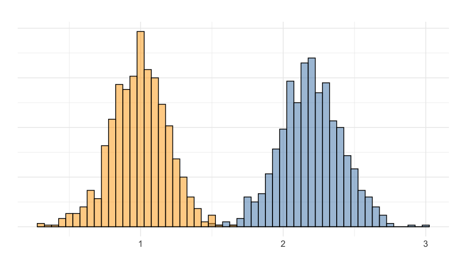
Figure 1: Bias in 2SLS. In orange the CF estimates, in blue the 2SLS estimates.

The result of Example 1 is further illustrated numerically in Figure 1, which contains, in blue, the empirical distribution of the 2SLS estimator, for a case where $\alpha=1$. The (asymptotic) bias is quite noticeable. As a preview of our results, our proposed estimators, correctly centered at $\alpha=1$, is shown in orange.

Next, we study the inconsistency of the 2SLS in more detail. In particular, we also assess the impact of heteroskedasticity in the first-stage equation.

2.3 Inconsistency of the 2SLS estimator

Next, we provide a formal result deriving the asymptotic bias in the 2SLS estimator. We maintain the following assumptions.

Assumption 1.

$(i)$ The sample ${(Y_{i},D_{i},X_{i}^{\prime},Z_{i}^{\prime})}_{i=1}^{n}$ is i.i.d. following the model (1)–(2). $(ii)$ The following exogeneity conditions hold: $E[\varepsilon|X,Z]=E[V|X,Z]=0$.

Assumption 2.

There is at least one component of $\pi_{1}$ which is not 0, and the matrices $E\begin{bmatrix}ZZ^{\prime}&ZX^{\prime}\\ XZ^{\prime}&XX^{\prime}\end{bmatrix}$ and $E\begin{bmatrix}XD&XX^{\prime}\\ ZD&ZX^{\prime}\end{bmatrix}$ have full column rank.

Assumptions 1 and 2 are standard in the literature allowing for endogeneity of $D$, the presence of observable controls $X$, as well as for the valid instruments $Z$ to be (intrinsically) exogenous.

While the instruments $Z$ are uncorrelated with $\varepsilon$ and $V$, we will see that when we consider the unobservable in (1) to be $g(D,X)\varepsilon$, then it might no longer be the case that $E[Zg(D,X)\varepsilon]=0$. That is, despite $Z$ being uncorrelated to the unobserved innovations, and being relevant, the heteroskedastic nature of the triangular system can invalidate the 2SLS procedure. As an alternative, we propose a control function approach in Section 3 below.

The next result compares the probability limit of the 2SLS estimator to the target parameter $\alpha_{1}$. We assume that the data is generated according to the model in (1)–(2), and a researcher who is interested in $\alpha_{1}$, instruments $D$ with $Z$ is a 2SLS regression of $Y$ of $D$ and $X$ (which includes a constant). In order to deal with the presence of the additional controls $X$, we use a population version of the Frisch-Waugh-Lovell (FWL) theorem using linear projections.

Lemma 1.

Consider the model in (1)–(2). Let $\overline{\alpha}_{1}$ be the probability limit of the 2SLS estimator of $\alpha_{1}$ of a 2SLS regression of $Y$ on $D$ and $X$, with $D$ instrumented by $Z$. Under Assumptions 1 and 2, we have

$$\overline{\alpha}_{1}=\alpha_{1}+\Sigma_{h}^{-1}\pi_{1}^{\prime}E[\overline{Z}g(Z^{\prime}\pi_{1}+X^{\prime}\pi_{2}+h(X,Z)V,X)\varepsilon],$$ (5)

where $\Sigma_{h}:=\pi_{1}^{\prime}E[\overline{Z}\,\overline{Z}^{\prime}]\pi_{1}$, and $\overline{Z}^{\prime}:=Z^{\prime}-X^{\prime}E[XX^{\prime}]^{-1}E[XZ^{\prime}]$.

We provide some further remarks to understand the intuition and nature of the result in Lemma 1.

1. The asymptotic bias of the 2SLS estimator in equation (5) can be succinctly written as $\Sigma_{h}^{-1}\pi_{1}^{\prime}E[\overline{Z}g(D,X)\varepsilon]$, but this might obscure the fact that $h(\cdot)$ is also playing a role through $D$.

2. If $g(\cdot)\equiv 1$, i.e., there is no heteroskedasticity in the structural equation, then there is no asymptotic bias in the 2SLS estimator because $E[\overline{Z}{g(D,X)\varepsilon}]=E[\overline{Z}{\varepsilon}]=0$ by Assumption 1. The lack of bias is regardless of $h(\cdot)$. For a general $g(\cdot)$, the form of $h(\cdot)$ may matter.

3. If $h(\cdot)\equiv 1$, i.e., there is no heteroskedasticity in the first-stage, then the asymptotic bias depends only on the form of $g(\cdot)$.

4. The strength of the instrumental variable, through the magnitude of $\pi_{1}$, can alleviate the bias. To see this, suppose that $d_{z}=1$. Then, the asymptotic bias is inversely related to $\pi_{1}$:

   $$\overline{\alpha}_{1}=\alpha_{1}+\frac{E[\overline{Z}{g(D,X)\varepsilon}]}{\pi_{1}E[\overline{Z}^{2}]}.$$

   Even in this simple case, the sign of the bias is not totally obvious.

5. If it is suspected that $b_{0}\leq E[\overline{Z}g(D,X)\varepsilon]\leq b_{1}$, then partial identification of $\alpha_{1}$ is possible. Otherwise, this can be used in a sensitivity analysis.

3 Identification: a control function approach

In this section, we propose sufficient conditions, together with a control function (CF) approach, to identify and estimate the parameters of interest in the model given in equations (1)–(2), in the presence of both endogeneity and general heteroskedasticity.

We maintain the following assumption.

Assumption 3.

Control Function Condition: $E(\varepsilon|D,X,Z)=E(\varepsilon|V)=r(V)$.

Assumption 3 is a standard control function condition, see, e.g., Blundell and Powell (2008) and Florens, Heckman, Meghir, and Vytlacil (2008). Under this condition, the conditional expectation of the response variable in equation (1) can be written as

$$E[Y|D,X,Z] =D\alpha_{1}+X^{\prime}\alpha_{2}+g(D,X)E[\varepsilon|D,X,Z]$$

$$=D\alpha_{1}+X^{\prime}\alpha_{2}+g(D,X)r(V).$$ (6)

It should be noted that, from the previous display, the skedastic term in the structural equation makes even the standard general identification procedures based on the control function fail. Further assumptions are required to identify $\alpha_{1}$. To illustrate this, we use Example 1 and follow the general identification method for nonparametric triangular models in Newey, Powell, and Vella (1999, Theorem 2.3). For simplicity, we assume that there are no additional exogenous covariates, $X$.

Example 2.

Consider the model in Example 1 and Assumption 3. Define

$$f(D,Z):=E[Y|D,Z] =D\alpha_{1}+g(D)E[\varepsilon|D,Z]$$

$$=D\alpha_{1}+g(D)r(V)$$

$$=D\alpha_{1}+g(D)r(\psi(D,Z)),$$

where $V:=\psi(D,Z)$ is an assumed identified control function from the first-stage. Now consider the following derivatives

$$\frac{\partial f}{\partial D} =\alpha_{1}+g_{D}r+gr_{V}\psi_{D}$$

$$\frac{\partial f}{\partial Z} =gr_{V}\psi_{Z},$$

where the derivatives are denoted by subscripts, and we omit the arguments in each function. The left hand-sides are identifiable. By multiplying the second equation of the above display by $\psi_{Z}^{\prime}(\psi_{Z}\psi_{Z}^{\prime})^{-1}$, and substituting the result into the first equation, we obtain

$$\frac{\partial f}{\partial D} =\alpha_{1}+g_{D}r+\frac{\partial f}{\partial Z}\psi_{Z}^{\prime}(\psi_{Z}\psi_{Z}^{\prime})^{-1}\psi_{D}.$$

Note, however, that one cannot identify $\alpha_{1}$ because of the additional term $g_{D}r$, that is,

$$\frac{\partial f}{\partial D}-\frac{\partial f}{\partial Z}\psi_{Z}^{\prime}(\psi_{Z}\psi_{Z}^{\prime})^{-1}\psi_{D} =\alpha_{1}+g_{D}r.$$ (7)

While the left-hand side of (7) contains only identified objects, the right-hand side contains three unknowns, $\alpha_{1}$, $g_{D}$ and $r$.

The previous example shows that further assumptions are required for identification of the parameter $\alpha_{1}$. The Assumption 4 below imposes a polynomial function on the skedastic function. This condition is the same as in Florens, Heckman, Meghir, and Vytlacil (2008), except that it includes additional exogenous covariates.

Assumption 4.

Polynomial Heteroskedasticity: $g(D,X)$ is a polynomial of degree $k_{g}$ in $D$ and $X$. That is $g(D,X)=1+\theta_{1}^{d}D+X^{\prime}\theta^{x}_{1}+...+\theta^{d}_{k_{g}}D^{k_{g}}+X^{\prime k_{g}}\theta^{x}_{k_{g}}$.

Here $X^{\prime k_{g}}$ refers to the element-by-element $k_{g}$ power of $X^{\prime}$. This could be replaced by any other polynomial that may include interactions. Finally, to make the model tractable, we impose the following polynomial structure on the CF. This simplifies identification, estimation, and inference.

Assumption 5.

Polynomial Control Function: $r(V)$ is a polynomial of degree $k_{v}$ in $V$ that does not contain a constant. That is $r(V)=\sum_{j=1}^{k_{v}}\mu_{j}V^{j}$.

An important condition in Assumption 5 is the exclusion of a constant term in the function $r(V)$. Otherwise, we may allow for $r(V)$ to include a constant, but restrict $g(D,X)$ to not contain a linear term with $D$ and $X$. The intuition for these restrictions is simple. Suppose there is only one endogenous regression $D$ and the both the skedastic function and the CF contain a constant as: $g(D)=1+\delta D$ and $r(V)=1+V$. Then, $g(D)r(V)=1+V+\delta D+\delta DV$, and in this case, one is not able to identify $\alpha_{1}$ because of the term $\delta D$. This is also highlighted by Florens, Heckman, Meghir, and Vytlacil (2008).

Identification of the parameter of interest requires identification of $V$, which in turn requires identification of $h$, which we can achieved up-to-scale. See for instance, Romano and Wolf (2017) and Wooldridge (2012, ch. 8) for parametric specifications, and Jin, Su, and Xiao (2015) and Linton and Xiao (2019) for nonparametric specifications. The next assumption imposes a normalization on the second moment of the control function, and requires the skedastic function to be positive.

Assumption 6.

Either $h\equiv 1$ or $E[V^{2}|X,Z]=1$ and $h(X,Z)>0$ almost surely.

The next lemma considers the identification of $\alpha_{1}$. It shows that the parameter of interest is identified by a regression of $Y$ on transformations of $(D,X,V)$.

Lemma 2.

Consider the regression

$$E[Y|D,X,Z] =D\alpha_{1}+X^{\prime}\alpha_{2}+\left(1+\sum_{s=1}^{k_{g}}(\theta_{s}^{d}D^{s}+X^{\prime s}\theta_{s}^{x})\right)\left(\sum_{j=1}^{k_{v}}\mu_{j}V^{j}\right),$$ (8)

and let $W$ denote all the regressors, but $D$. Under Assumptions 1–6, then $\alpha_{1}$ is identified as the coefficient of $D$ in the above regression and is given by

$$\alpha_{1} =\frac{E[(D-L_{D|W}(W))Y]}{E[(D-L_{D|W}(W))^{2}]},$$ (9)

provided $E[(D-L_{D|W}(W))^{2}]\neq 0$.

4 Estimation

This section proposes a practical estimator for the parameter of interest $\alpha_{1}$, and establishes its statistical limiting properties.

4.1 An augmented control function estimator

We consider an estimator that consists of a two-step procedure. The overall procedure is as following. In the first-stage, one estimates the control function (CF), $V$. In the second-stage, one performs a simple OLS regression of the dependent variable $Y$ on the regressors $(D,X^{\prime})^{\prime}$ and the estimated CF, $\widehat{V}$, as well as on their polynomial interactions.

The goal is to estimate $\alpha_{1}$ given in equation (9). Recall that from the identification results discussed in the previous section, the population parameter is given by

$$\alpha_{1}=\frac{E[(D-L_{D|W}(W))Y]}{E[(D-L_{D|W}(W))^{2}]},$$

where $W$ is defined as all the regressors on the right hand side of conditional average equation in (8), but $D$.

Denote the preliminary estimator of $V$ denoted by $\widehat{V}$. The estimator is given by

$$\widehat{\alpha}_{1}=\frac{\sum\limits_{i=1}^{n}(D_{i}-\widehat{L}_{[D|\widehat{W}]}(W_{i}))Y_{i}}{\sum_{i=1}^{n}(D_{i}-\widehat{L}_{[D|\widehat{W}]}(W_{i}))^{2}}.$$

where $\widehat{L}[D_{i}|\widehat{W}_{i}]=\widehat{W}_{i}^{\prime}(\widehat{W}^{\prime}\widehat{W})^{-1}\widehat{W}^{\prime}D.$ Here $\widehat{W}_{i}$ denotes the vector $W_{i}$ with $V_{i}$ replaced by $\widehat{V}_{i}$.

To implement this strategy in practice, we first estimate the errors in the first-stage regression. To this end, we employ OLS in the first-stage and regress the endogenous variable $D$ on the instruments, $Z$, and exogenous variables $X$, to compute the residuals

$$\widetilde{V}_{i} =D_{i}-Z_{i}^{\prime}\widehat{\pi}_{1}+X_{i}^{\prime}\widehat{\pi}_{2}.$$

Next, we have to compute the skedastic function $h(\cdot)$. Once we have an estimate of skedastic function, $\widehat{h}$, we obtain the normalized errors as

$$\widehat{V}_{i}=\widetilde{V}_{i}/\widehat{h}_{i},$$

where $\widehat{h}_{i}=h(X_{i},Z_{i})$ is the estimated skedastic function.

In practice, to estimate the skedastic function we employ the parametric models in Romano and Wolf (2017) or Wooldridge (2012, ch.8). For instance,

$$h(X,Z;\gamma)^{2}=|Z^{\prime}|\gamma_{1}+|X^{\prime}|\gamma_{2}.$$ (10)

or

$$h(X,Z;\gamma)^{2}=\exp\left(\log|Z^{\prime}|\gamma_{1}+\log|X^{\prime}|\gamma_{2}\right).$$ (11)

The coefficients of these models can be estimated using (possibly non-linear) OLS regressions with $\widetilde{V}^{2}_{i}$ as the dependent variable. The resulting estimator is $\widehat{h}_{i}=h(X_{i},Z_{i};\widehat{\gamma})$.

Finally, in the second-step a standard OLS estimation is performed by regressing the dependent variable $Y$ on the regressors $(D,X^{\prime})^{\prime}$, the estimated CF, $\widehat{V}$, and their polynomial interactions, $\widehat{W}$, as in (8).

4.2 Asymptotic properties

From equation (2), $V$ is given by

$$V(\phi) :=\frac{D-Z^{\prime}\pi_{1}-X^{\prime}\pi_{2}}{h(X,Z;\gamma)},$$ (12)

where $\phi:=(\pi_{1}^{\prime},\pi_{2}^{\prime},\gamma^{\prime})^{\prime}$. For notational brevity, we write equation (8) as

$$Y=D\alpha_{1}+W(\phi)^{\prime}\alpha_{w}+U,$$ (13)

where $W(\phi)$ contains all the regressors except $D$, and by construction, $E[U|D,W]=0$. The following assumption is used in the proposition below to derive the influence function of $\widehat{\phi}$ and to derive the asymptotic properties of $\alpha_{1}$, the parameter of interest.

Assumption 7.

(i) The map $\gamma\mapsto h(x,z;\gamma)$ is twice differentiable with gradient denoted by $\nabla_{\gamma}h(x,z;\gamma)$; (ii) $E[\nabla_{\gamma}h(X_{i},Z_{i};\gamma)\nabla_{\gamma}h(X_{i},Z_{i};\gamma)^{\prime}h(X_{i},Z_{i};\gamma)^{2}]$ has full rank; and (iii) the random vectors $Z_{i}h(X_{i},Z_{i})V_{i}$, $X_{i}h(X_{i},Z_{i})V_{i}$ and $\nabla_{\gamma}h(X_{i},Z_{i};\gamma)\left(V_{i}^{2}-1\right)h(X_{i},Z_{i};\gamma)^{3}$ have finite second moments.

Assumption 7 imposes a standard regularity condition on the skedastic function determining the smoothness and existence of moments of the conditional heteroskedasticity. The next result establishes a linear representation for the first-step estimator.

Proposition 1.

Under Assumptions 1, 2, 6, and 7, $\widehat{\phi}$ is asymptotically normal with influence function given by

$$\sqrt{n}(\widehat{\phi}-\phi) =\Sigma_{\phi}^{-1}\frac{1}{\sqrt{n}}\sum_{i=1}^{n}M_{i}+o_{p}(1),$$

where

$$\Sigma_{\phi}:=\begin{bmatrix}E[Z_{i}Z_{i}^{\prime}]&E[Z_{i}X_{i}^{\prime}]&0\\ E[X_{i}Z_{i}^{\prime}]&E[X_{i}X_{i}^{\prime}]&0\\ 0&0&2E[\nabla_{\gamma}h(X_{i},Z_{i};\gamma)\nabla_{\gamma}h(X_{i},Z_{i};\gamma)^{\prime}h(X_{i},Z_{i};\gamma)^{2}]\\ \end{bmatrix},$$

and

$$M_{i}=\begin{bmatrix}Z_{i}\left(D_{i}-Z_{i}^{\prime}\pi_{1}-X_{i}^{\prime}\pi_{2}\right)\\ X_{i}\left(D_{i}-Z_{i}^{\prime}\pi_{1}-X_{i}^{\prime}\pi_{2}\right)\\ \nabla_{\gamma}h(X_{i},Z_{i};\gamma)\left(V_{i}^{2}-1\right)h(X_{i},Z_{i};\gamma)^{3}\end{bmatrix}.$$

The next theorem contains the limiting distribution of the proposed two-step CF estimator of $\alpha$. This provides the details for the asymptotics for estimator of interest, which could be interpreted as an application of OLS with generated regressors. We consider the following assumption:

Assumption 8.

Let $W(\phi)$ be all the regressors in (13) (except $D$), and define $R_{i}(\phi):=(D_{i},W_{i}(\phi)^{\prime})^{\prime}$. Assume that uniformly in $\phi$ (i) $E[R_{i}(\phi)R_{i}^{\prime}(\phi)]$ is non-singular; (ii) a (uniform) law of large numbers holds for $\frac{1}{n}\sum_{i=1}^{n}R_{i}(\phi)R_{i}^{\prime}(\phi)$, $\frac{1}{n}\sum_{i=1}^{n}(U_{i}J_{\phi,i}-R_{i}(\phi)\alpha^{\prime}J_{\phi,i})$, where $J_{\phi}$ is the Jacobian of $\phi\mapsto R(\phi)$, $J_{\phi}=\nabla_{\phi}R(\phi)$; and (iii) $E[R^{2}U^{2}]<\infty$.

Assumption 8 $(i)$ ensures that the CF additional terms to the structural equation are not perfectly collinear to the main regressors, and Assumptions 8 $(ii)$ and $(iii)$ are required for the asymptotic representations using the influence functions.

Theorem 1.

Under Assumptions 1-8, $\widehat{\alpha}$ is asymptotically normal with influence function given by

$$\sqrt{n}(\widehat{\alpha}-\alpha) =\Sigma_{\alpha}^{-1}\frac{1}{\sqrt{n}}\sum_{i=1}^{n}\psi_{i}+o_{p}(1),$$

where $\Sigma_{\alpha}:=E[RR^{\prime}]$, $\psi_{i}:=R_{i}U_{i}+E[UJ_{\phi}-R(\phi)\alpha^{\prime}J_{\phi}]\Sigma_{\phi}^{-1}M_{i}$.

From the above result, we obtain

$$\sqrt{n}(\widehat{\alpha}_{1}-\alpha_{1})\stackrel{{\scriptstyle d}}{{\rightarrow}}\mathcal{N}(0,\Omega_{1}),$$

where $\Omega_{1}$ is the $(1,1)$ element of the limiting variance of $\sqrt{n}(\widehat{\alpha}-\alpha)$, denoted by $\Omega$, and is given by

$$\Omega=\Sigma_{\alpha}^{-1}\Psi\Sigma_{\alpha}^{-1}$$

with $\Psi=E[\psi\psi^{\prime}]$.

Estimation of $\Omega_{1}$ can be carried out by resorting to the sample counterpart of $\Omega$ as following:

$$\widehat{\Omega} =\widehat{\Sigma}_{\alpha}^{-1}\left[\frac{1}{n}\sum_{i=1}^{n}\left(\hat{\psi}_{i}\hat{\psi}_{i}^{\prime}\right)\right]\widehat{\Sigma}_{\alpha}^{-1},$$

where

$$\widehat{\Sigma}_{\alpha} =\frac{1}{n}\sum_{i=1}^{n}\widehat{R}_{i}\widehat{R}_{i}^{\prime},$$

$$\widehat{R}_{i} =R_{i}(\widehat{\phi}),$$

$$\widehat{U}_{i} =Y_{i}-D_{i}\widehat{\alpha}_{1}-W_{i}(\widehat{\phi})^{\prime}\widehat{\alpha}_{w},$$

$$\hat{\psi}_{i} =\hat{R}_{i}\hat{U}_{i}+\left[\frac{1}{n}\sum_{i=1}^{n}(\hat{U}_{i}\nabla_{\phi}R_{i}(\hat{\phi})-\hat{R}_{i}\hat{\alpha}^{\prime}\nabla_{\phi}R_{i}(\hat{\phi}))\right]\hat{\Sigma}_{\phi}^{-1}\hat{M}_{i},$$

$$\widehat{\Sigma}_{\phi} =\frac{1}{n}\sum_{i=1}^{n}\begin{bmatrix}Z_{i}Z_{i}^{\prime}&Z_{i}X_{i}^{\prime}&0\\ X_{i}Z_{i}^{\prime}&X_{i}X_{i}^{\prime}&0\\ 0&0&2[\nabla_{\gamma}h(X_{i},Z_{i};\widehat{\gamma})\nabla_{\gamma}h(X_{i},Z_{i};\widehat{\gamma})^{\prime}h(X_{i},Z_{i};\widehat{\gamma})^{2}]\\ \end{bmatrix},$$

$$\widehat{M}_{i} =\begin{bmatrix}Z_{i}\left(D_{i}-Z_{i}^{\prime}\widehat{\pi}_{1}-X_{i}^{\prime}\widehat{\pi}_{2}\right)\\ X_{i}\left(D_{i}-Z_{i}^{\prime}\widehat{\pi}_{1}-X_{i}^{\prime}\widehat{\pi}_{2}\right)\\ \nabla_{\gamma}h(X_{i},Z_{i};\widehat{\gamma})\left(\hat{V}_{i}^{2}-1\right)h(X_{i},Z_{i};\widehat{\gamma})^{3}\end{bmatrix}.$$

5 Monte Carlo Simulations

This section provides numerical simulations to assess the finite sample performance of the proposed methods. We use the following version of the model in equations (1) and (2),

$$Y =\alpha_{1}D+\alpha_{2}X+g(D,X)\varepsilon,$$ (14)

$$D =\pi_{1}Z+\pi_{2}X+h(Z,X)V,$$ (15)

$$\varepsilon =U+\lambda V.$$ (16)

This allows for endogeneity and different types of heteroskedasticity in both the first- and second-stages. The parameter $\lambda$ allows for $D$ being exogenous (i.e. $\lambda=0$) or endogenous (i.e. $\lambda\neq 0$) in the structural equation (14).

We compute simulation results for the cases of $U\sim N(0,1)$, $V\sim N(0,1)$, $Z$ following a folded normal distribution, that is $Z\sim|N(0,1)|$. Additionally, they are all independent of each other. We set $X\equiv 1$ so that all models have a constant term. Moreover, we use sample sizes of $n\in\{250,500,1000\}$. The number of replications is set to $2000$.

We consider different types of heteroskedastic models given by

$$g(D,X) =\delta_{1}D+\delta_{2}D^{2}+\delta_{3}X,$$ (17)

$$h(Z,X) =\gamma_{1}Z+\gamma_{2}X.$$ (18)

Parameters $(\delta_{1},\delta_{2})$ allow for heteroskedasticity of the endogenous variable in the structural equation (i.e. $\delta_{1}\neq 0$ or $\delta_{2}\neq 0$) and nonlinear effects (i.e. $\delta_{2}\neq 0$), while the parameter $\delta_{3}$ allows for heteroskedasticity of the exogenous variable, and in this case to have a constant term. Since the model includes a constant this ensures that the variance is not zero under the absence of endogenous heteroskedasticity. The parameter $\gamma_{1}$ also allows for $D$ having a conditional homoskedasticity (i.e. $\gamma_{1}=0$) or heteroskedasticity (i.e. $\gamma_{1}\neq 0$) in the first-stage equation (15). The parameters are $\alpha_{1}=\alpha_{2}=\pi_{1}=\pi_{2}=\delta_{3}=\gamma_{2}=1$, $\gamma_{1}\in\{0,1\}$, $\delta_{1}\in\{0,1\}$ and $\delta_{2}\in\{0,0.2\}$, thus covering a wide range of scenarios.

We present results for different estimators: OLS, standard 2SLS (note that this is equivalent to a standard CF model where $\tilde{V}$ is included as an additional regressor in the structural equation), and the proposed CF with one interaction term CF1 $(\widehat{V},\widehat{V}D)$, as well as with two interaction terms CF2 $(\widehat{V},\widehat{V}D,\widehat{V}D^{2})$.

For the CF models we consider one type of skedastic function that matches the data generating process (18) given in Romano and Wolf (2017), as given in equation (10), $h(X,Z;\gamma)^{2}=|Z^{\prime}|\gamma_{1}+|X^{\prime}|\gamma_{2}=\gamma_{0}+|Z^{\prime}|\gamma_{1}$, such that $\hat{h}=\sqrt{h(X,Z;\hat{\gamma})^{2}}$. Let $\tilde{V}$ be the residuals of the first-stage regression of $D$ on $Z$ and a constant, then $h^{2}$ is estimated as the regression of $\tilde{V}^{2}$ on $|Z|$ and a constant.

Tables 1 and 2 report the simulation results for the case of $\lambda=1$, i.e. endogeneity, for $\gamma_{1}=0$ and $\gamma_{1}=1$, respectively. For completeness Tables 3 and 4 report the simulation results for the case of $\lambda=0$, i.e. no endogeneity, also for $\gamma_{1}=0$ and $\gamma_{1}=1$, respectively. In all cases we report empirical bias and variance of the estimators OLS, 2SLS and CF estimators, and for the latter we compute the average of the estimated variance and 95% empirical coverage using the Gaussian confidence intervals.

The results in Tables 1 and 2 clearly indicate that OLS is biased and that 2SLS is also biased in the presence of endogenous heteroskedasticity (i.e. $\delta_{1}\neq 0$ and/or $\delta_{2}\neq 0$). Moreover, note that the parameter $\gamma_{1}$, i.e. heteroskedasticity in the first-stage, aggravates the 2SLS bias. However, the proposed CF estimators provide unbiased results. Note that this depends on the functional form of the heteroskedasticity-inducing function $g$. When $\delta_{2}=0$, both CF1 and CF2 works, but when $\delta_{2}=0.2$, only CF2 completely eliminates the bias. Overall, this indicates that the CF approach eliminates the bias, but nonlinear terms may be needed for different functional forms of the heteroskedasticity inducing functions $g$.

The last two columns of the tables provide the average estimated variance and the 95% coverage of the CF estimators. In all cases, the estimated variance gets close to the simulated variance and it is very similar when $n=1000$. Moreover, the empirical coverage is close to the 95% whenever we have an approximately unbiased estimator.

Tables 3 and 4 indicate that when there is no endogeneity and no correction is needed from OLS. the CF estimator is unbiased and behaves in a similar fashion to the 2SLS counterpart.

Table 1: Monte Carlo simulations, $\lambda=1$, $\gamma_{1}=0$

			OLS		2SLS		CF1 with $\hat{V}+\hat{V}\times D$
			Bias	Var.	Bias	Var.	Bias	Var.	Est.Var	Cov.95%
$n$	$\delta_{1}$	$\delta_{2}$
250	0	0	0.733	0.004	-0.016	0.026	-0.011	0.026	0.024	0.943
500	0	0	0.734	0.002	-0.006	0.011	-0.004	0.011	0.020	0.957
1000	0	0	0.735	0.001	0.000	0.005	0.001	0.005	0.006	0.958
250	0	0.2	1.806	0.060	0.368	0.216	0.382	0.192	0.325	0.828
500	0	0.2	1.805	0.030	0.382	0.104	0.389	0.094	0.093	0.714
1000	0	0.2	1.806	0.015	0.387	0.052	0.388	0.047	0.047	0.556
250	1	0	2.056	0.080	-0.037	0.337	-0.018	0.308	0.300	0.945
500	1	0	2.056	0.038	-0.010	0.151	-0.002	0.141	0.146	0.955
1000	1	0	2.051	0.019	-0.013	0.078	-0.008	0.071	0.072	0.951
250	1	0.2	3.131	0.216	0.372	0.777	0.403	0.693	2.236	0.894
500	1	0.2	3.123	0.105	0.373	0.368	0.384	0.327	0.340	0.888
1000	1	0.2	3.122	0.054	0.384	0.182	0.392	0.162	0.170	0.832
							CF2 with $\hat{V}+\hat{V}\times D+\hat{V}\times D^{2}$
250	0	0	0.730	0.004	-0.010	0.024	-0.006	0.026	0.032	0.934
500	0	0	0.732	0.002	-0.007	0.011	-0.006	0.012	0.012	0.946
1000	0	0	0.735	0.001	0.002	0.006	0.003	0.006	0.006	0.942
250	0	0.2	1.801	0.058	0.365	0.204	-0.020	0.164	0.172	0.951
500	0	0.2	1.804	0.029	0.385	0.105	-0.008	0.085	0.084	0.952
1000	0	0.2	1.807	0.015	0.391	0.050	-0.003	0.043	0.042	0.950
250	1	0	2.057	0.075	-0.047	0.309	-0.032	0.299	0.336	0.950
500	1	0	2.050	0.039	-0.015	0.164	-0.007	0.160	0.148	0.943
1000	1	0	2.048	0.019	-0.015	0.085	-0.008	0.081	0.074	0.942
250	1	0.2	3.127	0.208	0.344	0.754	-0.024	0.645	0.702	0.946
500	1	0.2	3.109	0.112	0.355	0.396	-0.029	0.334	0.333	0.949
1000	1	0.2	3.119	0.057	0.383	0.188	-0.025	0.166	0.165	0.946

Table 2: Monte Carlo simulations, $\lambda=1$, $\gamma_{1}=1$

			OLS		2SLS		CF1 with $\hat{V}+\hat{V}\times D$
			Bias	Var.	Bias	Var.	Bias	Var.	Est.Var	Cov.95%
$n$	$\delta_{1}$	$\delta_{2}$
250	0	0	0.614	0.003	-0.021	0.025	-0.009	0.023	0.116	0.943
500	0	0	0.612	0.001	-0.011	0.011	-0.005	0.011	0.011	0.953
1000	0	0	0.612	0.001	-0.004	0.006	-0.001	0.005	0.005	0.954
250	0	0.2	1.934	0.090	0.796	0.321	0.622	0.371	0.346	0.748
500	0	0.2	1.932	0.047	0.830	0.159	0.659	0.183	0.179	0.624
1000	0	0.2	1.942	0.025	0.850	0.086	0.678	0.101	0.094	0.379
250	1	0	1.835	0.066	0.305	0.337	-0.038	0.397	1.295	0.946
500	1	0	1.836	0.033	0.328	0.165	-0.017	0.192	0.191	0.945
1000	1	0	1.834	0.017	0.340	0.082	-0.017	0.097	0.094	0.946
250	1	0.2	3.147	0.271	1.135	1.059	0.620	1.185	1.071	0.864
500	1	0.2	3.167	0.149	1.182	0.487	0.663	0.553	0.564	0.838
1000	1	0.2	3.160	0.074	1.221	0.258	0.697	0.297	0.286	0.723
							CF2 with $\hat{V}+\hat{V}\times D+\hat{V}\times D^{2}$
250	0	0	0.612	0.002	-0.016	0.025	-0.006	0.026	0.053	0.946
500	0	0	0.614	0.001	-0.006	0.012	-0.002	0.012	0.012	0.944
1000	0	0	0.613	0.001	-0.006	0.006	-0.002	0.006	0.006	0.949
250	0	0.2	1.928	0.098	0.803	0.344	-0.029	0.289	0.649	0.940
500	0	0.2	1.940	0.052	0.841	0.166	-0.018	0.140	0.136	0.946
1000	0	0.2	1.940	0.024	0.845	0.083	-0.011	0.075	0.069	0.937
250	1	0	1.823	0.070	0.298	0.348	-0.044	0.406	2.308	0.939
500	1	0	1.830	0.033	0.322	0.165	-0.027	0.196	0.192	0.950
1000	1	0	1.834	0.017	0.332	0.079	-0.023	0.093	0.095	0.954
250	1	0.2	3.126	0.302	1.084	1.091	-0.097	1.062	1.057	0.940
500	1	0.2	3.140	0.137	1.138	0.513	-0.060	0.526	0.491	0.942
1000	1	0.2	3.176	0.075	1.221	0.251	0.011	0.252	0.247	0.952

Table 3: Monte Carlo simulations, $\lambda=0$, $\gamma_{1}=0$

			OLS		2SLS		CF1 with $\hat{V}+\hat{V}\times D$
			Bias	Var.	Bias	Var.	Bias	Var.	Est.Var	Cov.95%
$n$	$\delta_{1}$	$\delta_{2}$
250	0	0	0.000	0.003	0.001	0.012	0.001	0.012	0.011	0.945
500	0	0	0.000	0.002	-0.001	0.006	-0.001	0.006	0.006	0.941
1000	0	0	0.000	0.001	-0.001	0.003	-0.001	0.003	0.003	0.953
250	0	0.2	0.002	0.028	-0.001	0.098	-0.002	0.097	0.093	0.931
500	0	0.2	-0.005	0.015	-0.001	0.049	-0.001	0.049	0.046	0.939
1000	0	0.2	-0.003	0.007	-0.003	0.025	-0.003	0.025	0.024	0.942
250	1	0	-0.002	0.036	-0.010	0.152	-0.009	0.151	0.148	0.940
500	1	0	0.003	0.019	0.007	0.078	0.006	0.077	0.075	0.943
1000	1	0	0.000	0.010	0.006	0.040	0.006	0.040	0.037	0.936
250	1	0.2	-0.006	0.103	-0.009	0.379	-0.010	0.376	0.364	0.939
500	1	0.2	-0.004	0.051	-0.010	0.188	-0.011	0.187	0.176	0.944
1000	1	0.2	0.005	0.027	-0.004	0.094	-0.004	0.094	0.090	0.944
							CF2 with $\hat{V}+\hat{V}\times D+\hat{V}\times D^{2}$
250	0	0	0.001	0.003	0.001	0.012	0.002	0.014	0.013	0.947
500	0	0	0.001	0.001	0.002	0.006	0.002	0.007	0.007	0.943
1000	0	0	0.000	0.001	0.001	0.003	0.001	0.003	0.003	0.952
250	0	0.2	0.007	0.028	-0.007	0.096	-0.013	0.107	0.134	0.928
500	0	0.2	0.000	0.014	0.002	0.047	0.004	0.050	0.049	0.943
1000	0	0.2	0.002	0.007	0.000	0.023	0.000	0.024	0.025	0.952
250	1	0	0.006	0.039	0.024	0.163	0.026	0.179	0.315	0.936
500	1	0	-0.004	0.020	0.006	0.078	0.012	0.086	0.082	0.942
1000	1	0	0.000	0.009	0.003	0.039	0.005	0.043	0.041	0.951
250	1	0.2	-0.003	0.102	-0.012	0.365	-0.007	0.389	0.369	0.937
500	1	0.2	0.000	0.049	-0.005	0.181	-0.014	0.199	0.189	0.939
1000	1	0.2	-0.001	0.026	-0.009	0.091	-0.015	0.099	0.095	0.938

Table 4: Monte Carlo simulations, $\lambda=0$, $\gamma_{1}=1$

			OLS		2SLS		CF1 with $\hat{V}+\hat{V}\times D$
			Bias	Var.	Bias	Var.	Bias	Var.	Est.Var	Cov.95%
$n$	$\delta_{1}$	$\delta_{2}$
250	0	0	0.000	0.002	0.002	0.012	0.002	0.011	0.024	0.956
500	0	0	0.000	0.001	0.001	0.006	0.000	0.006	0.005	0.949
1000	0	0	0.000	0.000	0.000	0.003	0.000	0.003	0.003	0.948
250	0	0.2	-0.002	0.039	-0.006	0.151	-0.006	0.181	0.160	0.923
500	0	0.2	-0.001	0.020	-0.001	0.073	-0.002	0.091	0.086	0.935
1000	0	0.2	0.001	0.011	0.005	0.038	0.006	0.047	0.045	0.941
250	1	0	0.003	0.034	0.008	0.177	0.011	0.215	1.039	0.937
500	1	0	-0.002	0.017	-0.003	0.086	-0.003	0.104	0.099	0.937
1000	1	0	0.001	0.009	0.003	0.043	0.005	0.051	0.050	0.940
250	1	0.2	0.000	0.120	0.004	0.494	0.000	0.603	0.567	0.936
500	1	0.2	-0.006	0.061	-0.013	0.244	-0.016	0.301	0.291	0.944
1000	1	0.2	0.004	0.032	0.006	0.123	0.007	0.154	0.152	0.942
							CF2 with $\hat{V}+\hat{V}\times D+\hat{V}\times D^{2}$
250	0	0	0.001	0.002	0.005	0.012	0.004	0.013	0.048	0.951
500	0	0	0.000	0.001	0.001	0.006	0.002	0.007	0.006	0.945
1000	0	0	0.000	0.000	-0.001	0.003	0.000	0.003	0.003	0.943
250	0	0.2	-0.003	0.038	0.005	0.139	0.012	0.179	0.161	0.937
500	0	0.2	-0.001	0.020	-0.002	0.072	0.006	0.095	0.086	0.933
1000	0	0.2	0.000	0.009	0.001	0.035	0.007	0.050	0.045	0.927
250	1	0	-0.001	0.034	-0.003	0.173	-0.002	0.228	0.217	0.943
500	1	0	-0.002	0.017	-0.008	0.082	-0.011	0.110	0.108	0.943
1000	1	0	0.001	0.009	0.004	0.040	0.006	0.054	0.054	0.948
250	1	0.2	-0.003	0.132	-0.011	0.513	-0.010	0.637	0.713	0.926
500	1	0.2	-0.004	0.062	-0.006	0.257	-0.004	0.339	0.304	0.931
1000	1	0.2	-0.006	0.031	-0.008	0.125	-0.005	0.162	0.155	0.946

6 Empirical application

We apply the estimator to the study of the effect of public-sponsored training programs. As argued in LaLonde (1995), public programs of training and employment are designed to improve participant’s productive skills, which in turn would increase their earning potential and decrease dependency on social welfare benefits. We use data from the Job Training Partnership Act (JTPA) program, that has been extensively studied in the literature. For example, see Bloom, Orr, Bell, Cave, Doolittle, Lin, and Bos (1997) for a description, and Abadie, Angrist, and Imbens (2002) for applications. The JTPA was a large publicly-funded training program that began funding in October 1983 and continued until late 1990’s. We focus on the Title II subprogram, which was offered only to individuals with “barriers to employment” (long-term use of welfare, being a high-school drop-out, 15 or more recent weeks of unemployment, limited English proficiency, phsysical or mental disability, reading proficiency below 7th grade level or an arrest record). Individuals in the randomly assigned JTPA treatment group were offered training, while those in the control group were excluded for a period of 18 months. Our interest lies in measuring the effect of a training offer and actual training on of participants’ future earnings.

We use the database in Abadie, Angrist, and Imbens (2002) that contains information about adult male and female JTPA participants and non-participants. Let $Z$ denote the indicator variable for those receiving a JTPA offer. Of those offered, 60% completed the training; of those in the control group completion rate was less than 2%. The dependent variable $Y$ is the logarithm of 30 month accumulated earnings (we exclude individuals without earnings), $Z$ is a dummy variable for the JTPA offer, $D$ is the endogenous dummy variable corresponding to the JTPA training, $X$ is a set of exogenous covariates contaning individual characteristics. The parameter of interest is the effect of JTPA training on log earnings.

Next, we estimate the effect of JTPA training on log earnings. Results for different models appear in Table 5 where only the coefficient of JTPA training is reported. Besides OLS and 2SLS, we also consider several control function methods. We present estimate results for different estimates of heteroskedasticity in the first-stage (Heter. first-stage). The first column of results, where Heter. first-stage $h=1$, does not consider a skedastic function in the first-stage and uses just the residuals $\tilde{V}$. The second column (Heter. first-stage: $h=V^{2}$) applies a first-stage skedastic function using a regression of $\tilde{V}^{2}$ on all covariates. The third column (Heter. first-stage: $h=ln\ V^{2}$) repeats a similar exercise but using a regression of $log\ \tilde{V}^{2}$ on all covariates. Regarding the CF model, the first row uses the estimated CF from the first-stage ($\tilde{V}$). The second row considers the residual and its squared value ($\widehat{V}+\widehat{V^{2}}$). The third row adds the interaction with JTPA training to accommodate a given skedastic function in the structural equation ($\widehat{V}+\widehat{V}D$). The fourth row adds the interaction and the square ($\widehat{V}+\widehat{V}D+\widehat{V}^{2}$). Finally, the last row considers the case $\widehat{V}+\widehat{V}D+\widehat{V}^{2}+\widehat{V}^{2}D$. Standard errors are computed by bootstrap using 200 replications.

Table 5: Effect of JTPA training on log earnings

Heter. first-stage	$h=1$	$h=V^{2}$	$h=ln(V^{2})$
	0.266***
OLS	(0.0312)
	[0.198, 0.319]
	0.115**
2SLS	(0.0495)
	[0.022, 0.208]
Control function
	0.115**	0.242***	0.263***
$\hat{V}$	(0.0495)	(0.0452)	(0.0336)
	[0.022, 0.208]	[0.122, 0.306]	[0.191, 0.322]
	0.147**	0.186***	0.213***
$\hat{V}+\hat{V}^{2}$	(0.0696)	(0.0549)	(0.0462)
	[0.019, 0.276]	[0.070, 0.279]	[0.128, 0.308]
	0.165	0.189***	0.234***
$\hat{V}+\hat{V}D$	(0.104)	(0.0448)	(0.0379)
	[-0.039, 0.381]	[0.115, 0.291]	[0.160, 0.315]
	0.0450	0.200***	0.227***
$\hat{V}+\hat{V}D+\hat{V}^{2}$	(0.234)	(0.0555)	(0.0526)
	[-0.400, 0.478]	[0.090, 0.316]	[0.119, 0.323]
	-0.604	0.180***	0.235***
$\hat{V}+\hat{V}D+\hat{V}^{2}+\hat{V}^{2}D$	(0.463)	(0.0580)	(0.0559)
	[-1.486, 0.356]	[0.093, 0.313]	[0.108, 0.345]

Standard errors in parentheses using 200 bootstrap replications; 95 % percentile confidence interval in brackets.. *** p$<$0.01, ** p$<$0.05, * p$<$0.1.

The empirical results in Table 5 show that the OLS point estimate is 0.266, while the 2SLS estimate is 0.115. This shows a substantial decrease in effect of training on earning, which indicates that the 2SLS correction with respect to OLS might be too large. Next, we consider the control function estimates. Note that the result for the first row ($\widehat{V}$) and first column ($h=1$) coincides with 2SLS estimate. This is because in this case there is no heteroskedasticity in the first-stage, and the second-stage does not consider any interactions. The presence of heteroskedasticity documented before indicates that models using interactions as control function might be more appropriate. Thus, columns $h=V^{2}$ and $h=\ln(V^{2})$ are important. For the case where $\widehat{V}+\widehat{V}D$, the point estimate ranges from 0.189 to 0.234, depending on the first-stage correction (and discarding the model with no correction for heteroskedasticity in the first-stage). For the case $\widehat{V}+\widehat{V}D+\widehat{V}^{2}$ estimates range from 0.20 to 0.227, while for $\widehat{V}+\widehat{V}D+\widehat{V}^{2}+\widehat{V}^{2}D$ it ranges from 0.180 to 0.235. These cases show that results are robust to the inclusion of polynomial and interaction terms. Overall, the CF results show empirical evidence that the job training is effective in increasing earning, but estimates are more modest than those from simple OLS regressions.

7 Conclusion

This paper shows that the estimation of linear models with endogeneity using the popular two-stages least squares (2SLS) method may not be estimating the parameter of interest. In particular, in the presence of heteroskedasticity, something common when correcting the variance-covariance matrix and for doing correct inference, the 2SLS is inconsistent. The empirical literature has not paid specific attention to this issue, probably because the interest lied in estimating the LATE rather than the ATE, as popularized by the treatment effects agenda.

As an alternative we provide a simple to implement augmented control function estimator. The control function (CF) approach provides an intuitive modeling strategy to handle endogeneity (see Wooldridge (2015) for a review) and lies in the center of general approaches to this particular set-up (see Newey, Powell, and Vella (1999) and Florens, Heckman, Meghir, and Vytlacil (2008)). We show that this can be adapted to the least-squares linear estimation methods to correct for the 2SLS bias. In fact, the proposed solution is to augment the standard CF model (which corresponds to 2SLS) with interactions of the structural equation variables with the residuals from the first-stage.

An important future research is the extension of the methods developed in this paper to study panel data models.

Appendix

A.1 Interpretation of $\alpha_{1}$

It is important to attach an interpretation to the parameter $\alpha_{1}$ in the proposed set-up. To that end, define $y(d,x)$ to be the potential responses of the outcome to different values of the treatment, $d$, and covariates, $x$. Consider the following simple case:

$$y(d,x)=d\alpha_{1}+x^{\prime}\alpha_{2}.$$

First, we discuss the case where $d$ is binary. Then

$$y(1,x)-y(0,x)=\alpha_{1},$$

in which case the parameter of interest is the average treatment effect (ATE), because there is no treatment heterogeneity.

Alternatively, we could define the potential responses to be

$$y(d,x)=d\alpha_{1}+x^{\prime}\alpha_{2}+g(d,x)\epsilon,$$

and now we have heterogeneity, because

$$y(1,x)-y(0,x)=\alpha_{1}+(g(1,x)-g(0,x))\epsilon.$$

And then the ATE is

$$E[y(1,x)-y(0,x)] =\alpha_{1}+(g(1,x)-g(0,x))E[\epsilon]$$

$$=\alpha_{1}$$

if we assume that $E[\epsilon]=0$. This is similar to the approach taken by Abrevaya and Xu (2023), where the term $(g(1,x)-g(0,x))\epsilon$ reflects the variability/deviations from ATE for different individuals/subpopulations. As noted by those authors, the 2SLS bias, i.e. the discrepancy between the ATE and the LATE, depends on “the degree to which heteroskedasticity depends upon treatment, as well as the average error disturbance for the compliers” (p.4).

Now, consider the case where $D$ is allowed to take a continuum of values. Now, a more general modeling as in Florens, Heckman, Meghir, and Vytlacil (2008) might be useful. Consider the quantity

$$\frac{y(d+\Delta,x)-y(d,x)}{\Delta}=\alpha_{1}+\frac{g(d+\Delta,x)-g(d,x)}{\Delta}\epsilon,$$

and the ATE is $\alpha_{1}$ regardless of $d$, and the size of the jump $\Delta$. If this is the model, then this fits our 2SLS model in the example above.

An alternative is to model in the following way:

$$y(d,x)=\varphi(d)+x^{\prime}\alpha_{2}+g(d,x)\epsilon$$

for some smooth function $\varphi$. Now we have

$$\frac{y(d+\Delta,x)-y(d,x)}{\Delta}=\frac{\varphi(d+\Delta)-\varphi(d)}{\Delta}+\frac{g(d+\Delta,x)-g(d,x)}{\Delta}\epsilon,$$

and taking the limit we get

$$\lim_{\Delta\to 0}\frac{y(d+\Delta,x)-y(d,x)}{\Delta}=\varphi^{\prime}(d)+g^{\prime}(d,x)\epsilon,$$

and the ATE at $d$ is $\varphi^{\prime}(d)$, while the “average ATE” is $E[\varphi^{\prime}(D)]$. So a linear model

$$y=E[\varphi^{\prime}(D)]d+x^{\prime}\alpha_{2}+u$$

implies that

$$u=g(d,x)\epsilon+(\varphi(d)-E[\varphi^{\prime}(D)]d).$$

This is different from our model but it shows that the simple linear representation above can accommodate more general models.

A.2 Linear projections

Here we briefly review a few properties of linear projections. Let $Y$ be a random variable, and $X$ be a $d_{x}$-dimensional random vector which we assume always includes a constant. Define the linear projection of $Y$ onto $X$ at $x$ as

$$L_{[Y|X]}(x)=x^{\prime}E[XX^{\prime}]^{-1}E[XY].$$

Some properties of $L_{[Y|X]}$ are the following:

1. For any constants $a$ and $b$, then $L_{[aY+bW|X]}(x)=aL_{[Y|X]}(x)+bL_{[W|X]}(x)$.

2. The residual $\overline{Y}=Y-L_{[Y|X]}(X)$ is orthogonal to any linear function of $X$ in the following sense: for $\eta\in\mathbb{R}^{p_{x}}$ we have

   $$E[\eta^{\prime}X\overline{Y}] =E[\eta^{\prime}X(Y-L_{[Y|X]}(X))]$$

   $$=E[\eta^{\prime}XY-\eta^{\prime}XX^{\prime}E[XX^{\prime}]^{-1}E[XY]]$$

   $$=\eta^{\prime}E[XY]-\eta^{\prime}E[XX^{\prime}]E[XX^{\prime}]^{-1}E[XY]$$

   $$=\eta^{\prime}E[XY]-\eta^{\prime}E[XY]$$

   $$=0.$$

3. If $Y$ is $p_{y}$-dimensional with $p_{y}>1$, then we define:

   $$L_{[Y^{\prime}|X]}(x)=\underbrace{X^{\prime}}_{1\times p_{x}}\underbrace{E[XX^{\prime}]^{-1}}_{p_{x}\times p_{x}}\underbrace{E[XY^{\prime}]}_{p_{x}\times p_{y}}.$$

A.3 Proof of Lemma 1

First, with some abuse of notation, define the matrices (in the usual way) $M_{X}=I-X[X^{\prime}X]^{-1}X^{\prime}$ and $P_{M_{X}Z}=M_{X}Z[Z^{\prime}M_{X}Z]^{-1}Z^{\prime}M_{X}$. Let $\widehat{\alpha}_{1,2SLS}$ be the 2SLS estimator of a regression of $Y$ on $D$ and $X$, instrumented by $Z$:

$$\widehat{\alpha}_{1,2SLS}=(D^{\prime}P_{M_{X}Z}D)^{-1}D^{\prime}P_{M_{X}Z}Y.$$

The 2SLS is a minimum distance estimator — see Section 3.8 in Hayashi (2011) — based on the following moment condition: $E[\overline{Z}\,\overline{Y}]=E[\overline{Z}\,\overline{D}]\alpha_{1}$. The population version is the probability limit of $\widehat{\alpha}_{1,2SLS}$, and is given by

$$\overline{\alpha}_{1}=\left(E[\overline{Z}\,\overline{D}]^{\prime}E[\overline{Z}\,\overline{Z}^{\prime}]^{-1}E[\overline{Z}\,\overline{D}]\right)^{-1}E[\overline{Z}\,\overline{D}]^{\prime}E[\overline{Z}\,\overline{Z}^{\prime}]^{-1}E[\overline{Z}\,\overline{Y}].$$ (A.1)

Recall that the model is

$$Y =D\alpha_{1}+X^{\prime}\alpha_{2}+g(D,X)\varepsilon,$$

$$D =Z^{\prime}\pi_{1}+X^{\prime}\pi_{2}+h(X,Z)V.$$

Apply the linear projection operator to the structural equation:

$$L_{[Y|X]}(X) =L_{[D|X]}(X)\alpha_{1}+X^{\prime}\alpha_{2}+L_{[g(D,X)\varepsilon|X]}(X)$$

The residualized $Y$ is

$$\overline{Y} =\overline{D}\alpha_{1}+\overline{g\varepsilon},$$ (A.2)

where $g:=g(D,X)$ for notational simplicity. Plugging (A.2) into (A.1), we obtain

$$\overline{\alpha}_{1}=\alpha_{1}+\underbrace{\left(E[\overline{Z}\,\overline{D}]^{\prime}E[\overline{Z}\,\overline{Z}^{\prime}]^{-1}E[\overline{Z}\,\overline{D}]\right)^{-1}E[\overline{Z}\,\overline{D}]^{\prime}E[\overline{Z}\,\overline{Z}^{\prime}]^{-1}E[\overline{Z}\,\overline{g\varepsilon}]}_{\text{bias}}.$$ (A.3)

This is the general form of the bias, without taking into account the functional form relating $D$ to $Z$ and $X$. Note right away in (A.3), that if $g(D,X)\equiv 1$, then there is no bias, since $E[\overline{Z}\,\overline{\varepsilon}]=0$ by the validity of $Z$.

Apply a linear projection to the first-stage:

$$L_{[D|X]}(X) =L_{[Z^{\prime}\pi_{1}|X]}(X)+X^{\prime}\pi_{2}+L_{[h(X,Z)V|X]}(X)$$

Therefore, the residualized version is

$$\overline{D} =\overline{Z}^{\prime}\pi_{1}+\overline{hV}.$$ (A.4)

where $h:=h(X,Z)$ for notational simplicity. Now we plug-in (A.4) into the bias part of (A.3). First note that

$$E[\overline{Z}\,\overline{D}] =E[\overline{Z}\,\overline{Z}^{\prime}]\pi_{1}+E[\overline{Z}\,\overline{hV}]$$

$$=E[\overline{Z}\,\overline{Z}^{\prime}]\pi_{1},$$

because, by Assumption 1, $E[V|X,Z]=0$, which implies $E[\overline{Z}\,\overline{hV}]=0.$ So that

$$E[\overline{Z}\,\overline{D}]^{\prime}E[\overline{Z}\,\overline{Z}^{\prime}]^{-1}E[\overline{Z}\,\overline{g\varepsilon}] =\pi_{1}^{\prime}E[\overline{Z}\,\overline{Z}^{\prime}]E[\overline{Z}\,\overline{Z}^{\prime}]^{-1}E[\overline{Z}\,\overline{g\varepsilon}]$$

$$=\pi_{1}^{\prime}E[\overline{Z}\,\overline{g\varepsilon}].$$

Now for the other term in the bias

$$E[\overline{Z}\,\overline{D}]^{\prime}E[\overline{Z}\,\overline{Z}^{\prime}]^{-1}E[\overline{Z}\,\overline{D}] =\pi_{1}^{\prime}E[\overline{Z}\,\overline{Z}^{\prime}]E[\overline{Z}\,\overline{Z}^{\prime}]^{-1}E[\overline{Z}\,\overline{Z}^{\prime}]\pi_{1}$$

$$=\pi_{1}^{\prime}E[\overline{Z}\,\overline{Z}^{\prime}]\pi_{1}$$

$$=:\Sigma_{h}.$$

Putting all together we get that

$$\overline{\alpha}_{1}=\alpha_{1}+\Sigma_{h}^{-1}\pi_{1}^{\prime}E[\overline{Z}\,\overline{g\varepsilon}].$$

Now, since $g:=g(D,X)$, and $D=Z^{\prime}\pi_{1}+X^{\prime}\pi_{2}+h(X,Z)V,$ the final expression for the asymptotic bias is

bias $$=\Sigma_{h}^{-1}\pi_{1}^{\prime}E[\overline{Z}g(Z^{\prime}\pi_{1}+X^{\prime}\pi_{2}+h(X,Z)V,X)\varepsilon].$$

∎

A.4 Proof of Lemma 2

Since $h\equiv 1$, $V$ is identified from the first-stage in (2) as $V=D-Z^{\prime}\pi_{1}-X^{\prime}\pi_{2}$. Under Assumptions 3, 4, and 5, we have the following conditional expectation:

$$E[Y|D,X,Z] =D\alpha_{1}+X^{\prime}\alpha_{2}+\left(1+\sum_{s=1}^{k_{g}}(\theta_{s}^{d}D^{s}+X^{\prime s}\theta_{s}^{x})\right)\left(\sum_{j=1}^{k_{v}}\mu_{j}V^{j}\right).$$ (A.5)

Define $W$ to be all the regressors, but $D$, on the right hand side of (A.5). Then, we can write

$$Y =D\alpha_{1}+W^{\prime}\alpha_{w}+U$$ (A.6)

where $U:=Y-E[Y|D,W]$ and satisfies, by construction, $E[U|D,W]=0$. Now we use linear projections on $W$. By the projection of $Y$ on $W$ we have that $L_{Y|W}(W)=L_{D|W}(W)\alpha_{1}+W^{\prime}\alpha_{w}$, so that $Y-L_{Y|W}(W)=(D-L_{D|W}(W))\alpha_{1}+U.$ Since by assumption, $E[(D-L_{D|W}(W))^{2}]\neq 0$, then

$$\alpha_{1} =\frac{E[(D-L_{D|W}(W))(Y-L_{Y|W}(W))]}{E[(D-L_{D|W}(W))^{2}]}$$

$$=\frac{E[(D-L_{D|W}(W))Y]}{E[(D-L_{D|W}(W))^{2}]}.$$

If $h\nequiv 1$, then the first-stage in (2) is given by $D=Z^{\prime}\pi_{1}+X^{\prime}\pi_{2}+h(X,Z)V$. Consider the residual $h(X,Z)V$, and apply conditional expectations as follows:

$$E[h(X,Z)V|X,Z] =h(X,Z)E[V|X,Z]=0,$$ (A.7)

and

$$E[h(X,Z)^{2}V^{2}|X,Z] =h(X,Z)^{2}E[V^{2}|X,Z]=h(X,Z)^{2}.$$ (A.8)

where $E[V|X,Z]=0$ follows from Assumption 1, and $E[V^{2}|X,Z]=1$ follows from Assumption 6. Thus, it is in principle possible to identify $h(X,Z)$ in a two stage procedure. First, identify $h(X,Z)V$ as the residuals from the regression of $D$ on $Z$ and $X$, which is possible by (A.7). Second, following (A.8), run a regression of $h(X,Z)^{2}V^{2}$ on $X$ and $Z$ to obtain $h(X,Z)^{2}$. Finally, construct $V$ as

$$V=\frac{D-Z^{\prime}\pi_{1}-X^{\prime}\pi_{2}}{h(X,Z)},$$ (A.9)

which is possible since $h(X,Z)\neq 0$ almost surely. Once $V$ is identified, we can proceed as in the case where $h\equiv 1$. That is, $\alpha_{1}$ is identified by (9). ∎

A.5 Proof of Proposition 1

Here we are going to derive the influence function of $\sqrt{n}(\widehat{\phi}-\phi)$. The procedure is detailed in section 4.1, and we reproduce it here for completeness. Following (2), the first-stage equation is $D=Z^{\prime}\pi_{1}+X^{\prime}\pi_{2}+h(X,Z;\gamma)V.$ By Assumption 1, $E[V|X,Z]=0$, so that $E[D|X,Z]=Z^{\prime}\pi_{1}+X^{\prime}\pi_{2},$ and the OLS regression of $D$ on $Z$ and $X$ yields consistent estimators of $\pi_{1}$ and $\pi_{2}$, denoted by $\widehat{\pi}_{1}$ and $\widehat{\pi}_{2}$ respectively. That is, $\widehat{\pi}_{1}$ and $\widehat{\pi}_{2}$ satisfy the empirical moment condition:

$$\frac{1}{n}\sum_{i=1}^{n}\begin{bmatrix}Z_{i}\\ X_{i}\end{bmatrix}\left(D_{i}-Z_{i}^{\prime}\widehat{\pi}_{1}-X_{i}^{\prime}\widehat{\pi}_{2}\right)=0.$$ (A.10)

The residuals of the regression are denoted by $\widetilde{V}$, and are constructed as $\widetilde{V}_{i}=D_{i}-Z_{i}^{\prime}\widehat{\pi}_{1}-X_{i}^{\prime}\widehat{\pi}_{2}.$

To estimate $\gamma$, the parameter governing the skedastic function, a model needs to be chosen. Examples are given in equations (11) and (10): $h(X,Z;\gamma)^{2}=\exp\left(\gamma_{0}+\log|Z^{\prime}|\gamma_{1}+\log|X^{\prime}|\gamma_{2}\right)$, and $h(X,Z;\gamma)^{2}=\gamma_{0}+|Z^{\prime}|\gamma_{1}+|X^{\prime}|\gamma_{2}$ respectively. By assumption, $E[V^{2}|X,Z]=1$ and $h(X,Z;\gamma)\neq 0$ almost surely, so that by equation (2)

$$E[h(X,Z;\gamma)^{2}V^{2}|X,Z]=E[(D-Z^{\prime}\pi_{1}-X^{\prime}\pi_{2})^{2}|X,Z]=h(X,Z;\gamma)^{2}.$$

This means that a (possibly nonlinear) least squares regression of $(D-Z^{\prime}\pi_{1}-X^{\prime}\pi_{2})^{2}$ on a transformation of $Z$ and $X$ (given by either (11) or (10)) consistently estimates $\gamma$. This is, of course, unfeasible, so we use $\tilde{V}^{2}$. To be more precise, $\widehat{\gamma}$ is obtained as

$$\widehat{\gamma}=\arg\min_{a}\sum_{i=1}^{n}\left(\tilde{V}_{i}^{2}-h(X_{i},Z_{i};a)^{2}\right)^{2}$$ (A.11)

By Assumption 7, $\gamma\mapsto h(x,z;\gamma)$ is differentiable, then by the first order condition of (A.11), $\widehat{\gamma}$ satisfies

$$\frac{1}{n}\sum_{i=1}^{n}\nabla_{\gamma}h(X_{i},Z_{i};\widehat{\gamma})\left(\tilde{V}_{i}^{2}-h(X_{i},Z_{i};\widehat{\gamma})^{2}\right)h(X_{i},Z_{i};\widehat{\gamma})=o_{p}(n^{-1/2}),$$ (A.12)

where $\nabla_{\gamma}h(x,z;\widehat{\gamma})$ is the gradient of the map $\gamma\mapsto h(x,z;\gamma)$ evaluated at $\gamma=\widehat{\gamma}$. Combining the empirical moment conditions given in (A.10) and (A.12) we can write the two-step estimation problem in a single step with $(\widehat{\pi}_{1}^{\prime},\widehat{\pi}_{2}^{\prime},\widehat{\gamma}^{\prime})^{\prime}$ simultaneously satisfying

$$\frac{1}{n}\sum_{i=1}^{n}\begin{bmatrix}Z_{i}\left(D_{i}-Z_{i}^{\prime}\widehat{\pi}_{1}-X_{i}^{\prime}\widehat{\pi}_{2}\right)\\ X_{i}\left(D_{i}-Z_{i}^{\prime}\widehat{\pi}_{1}-X_{i}^{\prime}\widehat{\pi}_{2}\right)\\ \nabla_{\gamma}h(X_{i},Z_{i};\widehat{\gamma})\left((D_{i}-Z_{i}^{\prime}\widehat{\pi}_{1}-X_{i}^{\prime}\widehat{\pi}_{2})^{2}-h(X_{i},Z_{i};\widehat{\gamma})^{2}\right)h(X_{i},Z_{i};\widehat{\gamma})\end{bmatrix}=o_{p}(n^{-1/2}).$$ (A.13)

Next , we do a Taylor expansion of (A.13) around the true value of $\phi:=(\pi_{1}^{\prime},\pi_{2}^{\prime},\gamma^{\prime})^{\prime}$, apply of the law of large numbers, and multiply across by $\sqrt{n}$. To keep notation simple, recall that $D_{i}-Z_{i}^{\prime}\pi_{1}-X_{i}^{\prime}\pi_{2}=h(X_{i},Z_{i};\gamma)V_{i}$. This yields

$$o_{p}(1) =\frac{1}{\sqrt{n}}\sum_{i=1}^{n}\begin{bmatrix}Z_{i}\left(D_{i}-Z_{i}^{\prime}\pi_{1}-X_{i}^{\prime}\pi_{2}\right)\\ X_{i}\left(D_{i}-Z_{i}^{\prime}\pi_{1}-X_{i}^{\prime}\pi_{2}\right)\\ \nabla_{\gamma}h(X_{i},Z_{i};\gamma)\left(V_{i}^{2}-1\right)h(X_{i},Z_{i};\gamma)^{3}\end{bmatrix}$$

$$+E\begin{bmatrix}-Z_{i}Z_{i}^{\prime}&-Z_{i}X_{i}^{\prime}&0\\ -X_{i}Z_{i}^{\prime}&-X_{i}X_{i}^{\prime}&0\\ -2\nabla_{\gamma}h(X_{i},Z_{i};\gamma)V_{i}Z_{i}^{\prime}h(X_{i},Z_{i};\gamma)^{2}&-2\nabla_{\gamma}h(X_{i},Z_{i};\gamma)V_{i}X_{i}^{\prime}h(X_{i},Z_{i};\gamma)^{2}&\Sigma_{\gamma}\\ \end{bmatrix}\sqrt{n}\begin{bmatrix}\widehat{\pi}_{1}-\pi_{1}\\ \widehat{\pi}_{2}-\pi_{2}\\ \widehat{\gamma}-\gamma\end{bmatrix}.$$

Note that $E[-2\nabla_{\gamma}h(X_{i},Z_{i};\gamma)V_{i}Z_{i}^{\prime}h(X_{i},Z_{i};\gamma)^{2}]=E[-2\nabla_{\gamma}h(X_{i},Z_{i};\gamma)V_{i}X_{i}^{\prime}h(X_{i},Z_{i};\gamma)^{2}]=0$ because by Assumption 1, $E[V|X,Z]=0$. Also note that $E[\nabla_{\gamma}h(X_{i},Z_{i};\gamma)\left(V_{i}^{2}-1\right)h(X_{i},Z_{i};\gamma)^{3}]=0$ because we assumed $E[V^{2}|X,Z]=1$. The expression for $\Sigma_{\gamma}$ is

$$\Sigma_{\gamma}: =\frac{\partial}{\partial\gamma}\nabla_{\gamma}h(X_{i},Z_{i};\gamma)\left((D_{i}-Z_{i}^{\prime}\pi_{1}-X_{i}^{\prime}\pi_{2})^{2}-h(X_{i},Z_{i};\gamma)^{2}\right)h(X_{i},Z_{i};\gamma)$$

$$=\nabla^{2}_{\gamma\gamma}h(X_{i},Z_{i};\gamma)\left((D_{i}-Z_{i}^{\prime}\pi_{1}-X_{i}^{\prime}\pi_{2})^{2}-h(X_{i},Z_{i};\gamma)^{2}\right)h(X_{i},Z_{i};\gamma)$$

$$-2\nabla_{\gamma}h(X_{i},Z_{i};\gamma)\nabla_{\gamma}h(X_{i},Z_{i};\gamma)^{\prime}h(X_{i},Z_{i};\gamma)^{2}$$

$$+\nabla_{\gamma}h(X_{i},Z_{i};\gamma)\nabla_{\gamma}h(X_{i},Z_{i};\gamma)^{\prime}\left((D_{i}-Z_{i}^{\prime}\pi_{1}-X_{i}^{\prime}\pi_{2})^{2}-h(X_{i},Z_{i};\gamma)^{2}\right).$$

Because $E[(D-Z^{\prime}\pi_{1}-X^{\prime}\pi_{2})^{2}|X,Z]=h(X,Z_{;}\gamma)^{2}$, $E[\Sigma_{\gamma}]$ simplifies to

$$E[\Sigma_{\gamma}]=-2E[\nabla_{\gamma}h(X_{i},Z_{i};\gamma)\nabla_{\gamma}h(X_{i},Z_{i};\gamma)^{\prime}h(X_{i},Z_{i};\gamma)^{2}].$$

Thus, we have that

$$o_{p}(1) =\frac{1}{\sqrt{n}}\sum_{i=1}^{n}\begin{bmatrix}Z_{i}\left(D_{i}-Z_{i}^{\prime}\pi_{1}-X_{i}^{\prime}\pi_{2}\right)\\ X_{i}\left(D_{i}-Z_{i}^{\prime}\pi_{1}-X_{i}^{\prime}\pi_{2}\right)\\ \nabla_{\gamma}h(X_{i},Z_{i};\gamma)\left(V_{i}^{2}-1\right)h(X_{i},Z_{i};\gamma)^{3}\end{bmatrix}$$

$$+\begin{bmatrix}-E[Z_{i}Z_{i}^{\prime}]&-E[Z_{i}X_{i}^{\prime}]&0\\ -E[X_{i}Z_{i}^{\prime}]&-E[X_{i}X_{i}^{\prime}]&0\\ 0&0&-2E[\nabla_{\gamma}h(X_{i},Z_{i};\gamma)\nabla_{\gamma}h(X_{i},Z_{i};\gamma)^{\prime}h(X_{i},Z_{i};\gamma)^{2}]\\ \end{bmatrix}\sqrt{n}\begin{bmatrix}\widehat{\pi}_{1}-\pi_{1}\\ \widehat{\pi}_{2}-\pi_{2}\\ \widehat{\gamma}-\gamma\end{bmatrix}.$$

Therefore, the influence function of $\sqrt{n}(\widehat{\phi}-\phi)$ is

$$\sqrt{n}(\widehat{\phi}-\phi) =\begin{bmatrix}E[Z_{i}Z_{i}^{\prime}]&E[Z_{i}X_{i}^{\prime}]&0\\ E[X_{i}Z_{i}^{\prime}]&E[X_{i}X_{i}^{\prime}]&0\\ 0&0&2E[\nabla_{\gamma}h(X_{i},Z_{i};\gamma)\nabla_{\gamma}h(X_{i},Z_{i};\gamma)^{\prime}h(X_{i},Z_{i};\gamma)^{2}]\\ \end{bmatrix}^{-1}$$

$$\frac{1}{\sqrt{n}}\sum_{i=1}^{n}\begin{bmatrix}Z_{i}\left(D_{i}-Z_{i}^{\prime}\pi_{1}-X_{i}^{\prime}\pi_{2}\right)\\ X_{i}\left(D_{i}-Z_{i}^{\prime}\pi_{1}-X_{i}^{\prime}\pi_{2}\right)\\ \nabla_{\gamma}h(X_{i},Z_{i};\gamma)\left(V_{i}^{2}-1\right)h(X_{i},Z_{i};\gamma)^{3}\end{bmatrix}+o_{p}(1).$$

Since the matrix above is block diagonal, then we have

$$\sqrt{n}(\widehat{\phi}-\phi) =\begin{bmatrix}\begin{bmatrix}E[Z_{i}Z_{i}^{\prime}]&E[Z_{i}X_{i}^{\prime}]\\ E[X_{i}Z_{i}^{\prime}]&E[X_{i}X_{i}^{\prime}]\end{bmatrix}^{-1}&0\\ 0&\frac{1}{2}E[\nabla_{\gamma}h(X_{i},Z_{i};\gamma)\nabla_{\gamma}h(X_{i},Z_{i};\gamma)^{\prime}h(X_{i},Z_{i};\gamma)^{2}]^{-1}\\ \end{bmatrix}$$

$$\frac{1}{\sqrt{n}}\sum_{i=1}^{n}\begin{bmatrix}Z_{i}\left(D_{i}-Z_{i}^{\prime}\pi_{1}-X_{i}^{\prime}\pi_{2}\right)\\ X_{i}\left(D_{i}-Z_{i}^{\prime}\pi_{1}-X_{i}^{\prime}\pi_{2}\right)\\ \nabla_{\gamma}h(X_{i},Z_{i};\gamma)\left(V_{i}^{2}-1\right)h(X_{i},Z_{i};\gamma)^{3}\end{bmatrix}+o_{p}(1).$$

The inverses of the blocks exists because of Assumptions 2 and 7. Asymptotic normality follows from Assumption 7 by the second moments being finite. ∎

A.6 Proof of Theorem 1

The goal is to establish the limiting distribution of the OLS estimators of the following regression given in (A.5) and (A.6):

$$Y =D\alpha_{1}+X^{\prime}\alpha_{2}+\left(1+\sum_{s=1}^{k_{g}}(\theta_{s}^{d}D^{s}+X^{\prime s}\theta_{s}^{x})\right)\left(\sum_{j=1}^{k_{v}}\mu_{j}V^{j}\right)+U$$ (A.14)

$$=D\alpha_{1}+W^{\prime}\alpha_{w}+U,$$

where $U:=Y-E[Y|D,W]$ and satisfies, by construction, $E[U|D,W]=0$. We follow Appendix 6A in Wooldridge (2010) closely. To implement the regression, $V$ is replaced by $\widehat{V}$. Recall that, according to (A.9), $V$ is given by

$$V(\phi) =\frac{D-Z^{\prime}\pi_{1}-X^{\prime}\pi_{2}}{h(X,Z;\gamma)},$$

where $\phi:=(\pi_{1}^{\prime},\pi_{2}^{\prime},\gamma^{\prime})^{\prime}$. The estimated counterpart, detailed in Section 4.1, is

$$\widehat{V} =V(\widehat{\phi})$$

$$=\frac{D-Z^{\prime}\widehat{\pi}_{1}-X^{\prime}\widehat{\pi}_{2}}{h(X,Z;\widehat{\gamma})}.$$

Let $W(\phi)$ be all the regressors in (A.14) (except $D$), and let $W(\widehat{\phi})=\widehat{W}$ denote those regressor where $V$ is replaced by the generated $\widehat{V}.$ In terms of the regression in equation (A.14), this is

$$W^{\prime}\alpha_{w}=W(\phi)^{\prime}\alpha_{w}=X^{\prime}\alpha_{2}+\left(1+\sum_{s=1}^{k_{g}}(\theta_{s}^{d}D^{s}+X^{\prime s}\theta_{s}^{x})\right)\left(\sum_{j=1}^{k_{v}}\mu_{j}V(\phi)^{j}\right),$$

and

$$\widehat{W}^{\prime}\alpha_{w}=W(\widehat{\phi})^{\prime}\alpha_{w}=X^{\prime}\alpha_{2}+\left(1+\sum_{s=1}^{k_{g}}(\theta_{s}^{d}D^{s}+X^{\prime s}\theta_{s}^{x})\right)\left(\sum_{j=1}^{k_{v}}\mu_{j}V(\widehat{\phi})^{j}\right).$$

Furthermore, let $R_{i}(\phi):=(D_{i},W_{i}(\phi)^{\prime})^{\prime}$ and $R_{i}(\widehat{\phi})=\widehat{R}_{i}:=(D_{i},\widehat{W}_{i}^{\prime})^{\prime}$. Also denote $\alpha:=(\alpha_{1},\alpha_{w}^{\prime})^{\prime}$, and $\widehat{\alpha}:=(\widehat{\alpha}_{1},\widehat{\alpha}_{w}^{\prime})^{\prime}$, where $\widehat{\alpha}_{1}$, and $\widehat{\alpha}_{w}$ are the OLS estimators of the regression of $Y$ on $D$ and $\widehat{W}$.

If $\phi$ were known, then the influence function of $\alpha$ would be given by $\Sigma_{\alpha}^{-1}R_{i}(\phi)U_{i}$ where $\Sigma_{\alpha}:=E[R_{i}(\phi)R_{i}(\phi)^{\prime}]$. To account for the influence of estimating $\phi$ we need to evaluate the effect is has on $R(\phi)U=R(\phi)(Y-R(\phi)^{\prime}\alpha)$.

For this we need first to compute $J_{\phi,i}=\nabla_{\phi}R_{i}(\phi)$, that is, the derivative of $R(\phi)$ with respect to $\phi$, a $dim(R)\times dim(\phi)$ matrix.

Write (A.13) succintly as

$$\frac{1}{n}\sum_{i=1}^{n}m_{i}(\widehat{\phi})=o_{p}(n^{-1/2}).$$

Combining this with the first order condition for the OLS estimation of $\alpha$, we get

$$\frac{1}{n}\sum_{i=1}^{n}\begin{bmatrix}m_{i}(\widehat{\phi})\\ R_{i}(\widehat{\phi})(Y_{i}-R_{i}(\widehat{\phi})^{\prime}\widehat{\alpha})\end{bmatrix}=o_{p}(n^{-1/2}).$$

Focusing on the second step estimation, we get using Assumption 8:

$$\frac{1}{n}\sum_{i=1}^{n}R_{i}(\widehat{\phi})(Y_{i}-R_{i}(\widehat{\phi})^{\prime}\widehat{\alpha}) =\frac{1}{n}\sum_{i=1}^{n}R_{i}(\phi)(Y_{i}-R_{i}(\phi)^{\prime}\widehat{\alpha})+\frac{1}{n}\sum_{i=1}^{n}(U_{i}J_{\phi,i}-R_{i}(\phi)\alpha^{\prime}J_{\phi,i})(\widehat{\phi}-\phi)+o_{p}(n^{-1/2}),$$

$$=\frac{1}{n}\sum_{i=1}^{n}R_{i}(\phi)(Y_{i}-R_{i}(\phi)^{\prime}\widehat{\alpha})+E[UJ_{\phi}-R(\phi)\alpha^{\prime}J_{\phi}](\widehat{\phi}-\phi)+o_{p}(n^{-1/2}),$$

$$=\Sigma_{\alpha}(\widehat{\alpha}-\alpha)+E[UJ_{\phi}-R(\phi)\alpha^{\prime}J_{\phi}](\widehat{\phi}-\phi)+o_{p}(n^{-1/2}).$$

Let

$$\psi_{i}=R_{i}U_{i}+E[UJ_{\phi}-R(\phi)\alpha^{\prime}J_{\phi}]\Sigma_{\phi}^{-1}M_{i}$$

and $\Psi:=E[\psi\psi^{\prime}]$. Therefore,

$$\sqrt{n}(\widehat{\alpha}-\alpha) =\Sigma_{\alpha}^{-1}\frac{1}{\sqrt{n}}\sum_{i=1}^{n}\psi_{i}+o_{p}(1),$$

and

$$\sqrt{n}(\widehat{\alpha}-\alpha)\stackrel{{\scriptstyle d}}{{\rightarrow}}\mathcal{N}(0,\Sigma_{\alpha}^{-1}\Psi\Sigma_{\alpha}^{-1}).$$

∎

References

- (1)
- Abadie, Angrist, and Imbens (2002) Abadie, A., J. Angrist, and G. Imbens (2002): “Instrumental Variables Estimates of the Effect of Subsidized Training on the Quantiles of Trainee Earnings,” Econometrica, 70, 91–117.
- Abrevaya and Xu (2023) Abrevaya, J., and H. Xu (2023): “Estimation of Treatment Effects under Endogenous Heteroskedasticity,” Journal of Econometrics, 234, 451–478.
- Arellano (1987) Arellano, M. (1987): “Computing Robust Standard Errors for Within-Groups Estimators,” Oxford Bulletin of Economics and Statistics, 49, 431–434.
- Bertrand, Duflo, and Mullainathan (2004) Bertrand, M., E. Duflo, and S. Mullainathan (2004): “How Much Should We Trust Differences-in-Differences Estimates?,” Quarterly Journal of Economics, 119, 249–275.
- Bloom, Orr, Bell, Cave, Doolittle, Lin, and Bos (1997) Bloom, H. S. B., L. L. Orr, S. H. Bell, G. Cave, F. Doolittle, W. Lin, and J. M. Bos (1997): “The Benefits and Costs of JTPA Title II-A programs. Key Findings from the National Job Training Partnership Act Study,” Journal of Human Resources, 32, 549–576.
- Blundell and Powell (2008) Blundell, R., and J. Powell (2008): “Endogeneity in Nonparametric and Semiparametric Regression Models,” in Advances in Economics and Econometrics Theory and Applications, Eighth World Congress, ed. by M. Dewatripont, L. P. Hansen, and S. J. Turnovsky, pp. 1–12. Cambridge: Cambridge University Press.
- Cameron and Miller (2015) Cameron, A. C., and D. L. Miller (2015): “A Practitioner’s Guide to Cluster-Robust Inference,” Journal of Human Resources, 50, 317–372.
- Carlson (2023) Carlson, A. (2023): “Relaxing Conditional Independence in an Endogenous Binary Response Model,” Journal of Econometrics, 232, 490–500.
- Chen, Khan, and Tang (2024) Chen, S., S. Khan, and X. Tang (2024): “Endogeneity in Weakly Separable Models without Monotonicity,” Journal of Econometrics, 238, 105567.
- Chen and Khan (2014) Chen, S. H., and S. Khan (2014): “Semi-Parametric Estimation of Program Impacts on Dispersion of Potential Wages,” Journal of Applied Econometrics, 29, 901–919.
- Chesher (2003) Chesher, A. (2003): “Identification in Nonseparable Models,” Econometrica, 71, 1405–1441.
- D’Haultfœuille and Février (2015) D’Haultfœuille, X., and Février (2015): “Identification of Nonseparable Triangular Models with Discrete Instruments,” Econometrica, 83, 1199–1210.
- Donald and Lang (2007) Donald, S. G., and K. Lang (2007): “Inference with Difference-in-Differences and Other Panel Data,” Review of Economics and Statistics, 89(2), 221–233.
- Florens, Heckman, Meghir, and Vytlacil (2008) Florens, J. P., J. J. Heckman, C. Meghir, and E. Vytlacil (2008): “Identification of Treatment Effects Using Control Functions in Models with Continuous, Endogenous Treatment and Heterogeneous Effects,” Econometrica, 76(5), 1191–1206.
- Hahn, Todd, and Van der Klaauw (2001) Hahn, J., P. Todd, and W. Van der Klaauw (2001): “Identification and Estimation of Treatment Effects with a Regression-Discontinuity Design,” Econometrica, 69, 201–209.
- Han (2020) Han, S. (2020): “Nonparametric Estimation of Triangular Simultaneous Equations Models under Weak Identification,” Quantitative Economics, 11, 161–202.
- Hansen (2007) Hansen, C. B. (2007): “Asymptotic Properties of a Robust Variance Matrix Estimator for Panel Data When is Large,” Journal of Econometrics, 141, 597–620.
- Hausman (1983) Hausman, J. (1983): “Specification and Estimation of Simultaneous Equations Models,” in Handbook of Econometrics Vol. 1., ed. by Z. Griliches, and M. Intriligator, pp. 391–448. North-Holland.
- Hayashi (2011) Hayashi, F. (2011): Econometrics. Princeton University Press.
- Heckman, Smith, and Clements (1997) Heckman, J., J. Smith, and N. Clements (1997): “Making the Most Out of Programme Evaluations and Social Experiments: Accounting for Heterogeneity in Programme Impacts,” Review of Economic Studies, 64, 487–535.
- Heckman and Vytlacil (2005) Heckman, J., and E. Vytlacil (2005): “Structural Equations, Treatment Effects, and Econometric Policy Evaluation,” Econometrica, 73, 669–738.
- Heckman and Vytlacil (2007) (2007): “Econometric Evaluation of Social Programs, Part I: Causal Models, Structural models and Econometric Policy Evaluation,” in Handbook of Econometrics Vol. 6., ed. by J. J. Heckman, and E. E. Leamer, pp. 4779–4874. Elsevier.
- Imbens and Angrist (1994) Imbens, G., and J. Angrist (1994): “Identification and Estimation of Local Average Treatment Effects,” Econometrica, 62, 467–475.
- Imbens and Newey (2009) Imbens, G. W., and W. K. Newey (2009): “Identification and Estimation of Triangular Simultaneous Equations Models Without Additivity,” Econometrica, 77(5), 1481–1512.
- Jennrich (1969) Jennrich, R. I. (1969): “Asymptotic Properties of Non-Linear Least Squares Estimators,” The Annals of Mathematical Statistics, 40(2), 633–643.
- Jin, Su, and Xiao (2015) Jin, S., L. Su, and Z. Xiao (2015): “Adaptive Nonparametric Regression with Conditional Heteroskedasticity,” Econometric Theory, 31, 1153–1191.
- Kézdi (2004) Kézdi, G. (2004): “Robust Standard Error Estimation in Fixed-Effects Panel Models,” Hungarian Statistical Review, 9, 95–116.
- Kim and Petrin (2022) Kim, K. i., and A. Petrin (2022): “A Generalized Non-parametric Instrumental Variable-Control Function Approach to Estimation in Nonlinear Settings,” Journal of Econometric Methods, 11, 91–125.
- LaLonde (1995) LaLonde, R. J. (1995): “The Promise of Public-Sponsored Training Programs,” Journal of Economic Perspectives, 9, 149–168.
- Lee (2007) Lee, S. (2007): “Endogeneity in Quantile Regression Models: a Control Function Approach,” Journal of Econometrics, 141, 1131–1158.
- Linton and Xiao (2019) Linton, O., and Z. Xiao (2019): “Efficient Estimation of Nonparametric Regression in the Presence of Dynamic Heteroskedasticity,” Journal of Econometrics, 213, 608–631.
- Ma and Koenker (2006) Ma, L., and R. Koenker (2006): “Quantile Regression Methods for Recursive Structural Equation Models,” Journal of Econometrics, 134(2), 471–506.
- Mogstad, Torgovitsky, and Walters (2021) Mogstad, M., A. Torgovitsky, and C. R. Walters (2021): “The Causal Interpretation of Two-Stage Least Squares with Multiple Instrumental Variables,” American Economic Review, 111, 3663–3698.
- Newey and McFadden (1994) Newey, W. K., and D. L. McFadden (1994): “Large Sample Estimation and Hypothesis Testing,” in Handbook of Econometrics, ed. by R. F. Engle, and D. L. McFadden, vol. 4, pp. 2111–2245. Elsevier.
- Newey and Powell (2003) Newey, W. K., and J. L. Powell (2003): “Instrumental Variable Wstimation of Nonparametric Models,” Econometrica, 71, 1565–1578.
- Newey, Powell, and Vella (1999) Newey, W. K., J. L. Powell, and F. Vella (1999): “Nonparametric Estimation of Triangular Simultaneous Equations Models,” Econometrica, 67, 565–603.
- Newey and West (1987) Newey, W. K., and K. D. West (1987): “A Simple, Positive Semi-Definite, Heteroskedasticity and Autocorrelation Consistent Covariance Matrix,” Econometrica, 55, 703–708.
- Pagan and Hall (1983) Pagan, A., and A. Hall (1983): “Diagnostic Tests as Residual Analysis,” Econometric Reviews, 2(2), 159–218.
- Pereda-Fernández (2023) Pereda-Fernández, S. (2023): “Identification and Estimation of Triangular Models with a Binary Treatment,” Journal of Econometrics, 234(2), 585–623.
- Raj, Srivastava, and Ullah (1980) Raj, B., V. K. Srivastava, and A. Ullah (1980): “Generalized Two Stage Least Squares Estimators for a Structural Equation with Both Fixed and Random Coefficients,” International Economic Review, 21, 171–183.
- Romano and Wolf (2017) Romano, J. P., and M. Wolf (2017): “Resurrecting Weighted Least Squares,” Journal of Econometrics, 197, 1–19.
- Torgovitsky (2015) Torgovitsky, A. (2015): “Identification of Nonseparable Models Using Instruments with Small Support,” Econometrica, 83, 1185–1197.
- van der Vaart (1998) van der Vaart, A. (1998): Asymptotic Statistics. Cambridge University Press, Cambridge.
- White (1980) White, H. (1980): “A Heteroskedasticity-Consistent Covariance Matrix Estimator and a Direct Test for Heteroskedasticity,” Econometrica, 48, 817–838.
- White (1982) (1982): “Instrumental Variables Regression with Independent Observations,” Econometrica, 50, 483–499.
- Wooldridge (1997) Wooldridge, J. M. (1997): “On Two Stage Least Squares Estimation of the Average Treatment Effect in a Random Coefficient Model,” Economics Letters, 56, 129–133.
- Wooldridge (2003a) (2003a): “Cluster-Sample Methods in Applied Econometrics,” American Economic Review, 93, 133–138.
- Wooldridge (2003b) (2003b): “Further Results on Instrumental Variables Estimation of the Average Treatment Effect in a random Coefficient Model,” Economics Letters, 79, 185–191.
- Wooldridge (2010) (2010): Econometric Analysis of Cross Section and Panel Data. MIT Press, 2nd Edition.
- Wooldridge (2012) (2012): Introductory Econometrics: A Modern Approach. South-Western, 2nd Edition.
- Wooldridge (2015) (2015): “Control Function Methods in Applied Econometrics,” The Journal of Human Resources, 50(2), 420–445.