Deep in the Knotted Black Hole
Abstract
We consider the transition rate of a freely falling Unruh-DeWitt (UDW) detector, coupled linearly to a massless scalar quantum field prepared in the Hartle-Hawking-Israel state, as a probe of the interior of a black hole. Specifically, we consider the transition rate of a detector in the spinless Bañados-Teitelboim-Zanelli (BTZ) black hole as it freely falls toward and across the horizon and compare it to the corresponding situation for an geon. Both the BTZ black hole and its geon counterpart are quotients of spacetime that are identical exterior to the horizon but have different interior topologies. We find outside the horizon that the rates are qualitatively similar, but with the amplitude in the geon spacetime larger than in the BTZ case. Once the detector crosses the horizon, there are notable distinctions characterized by different discontinuities in the temporal derivative of the response rate. These discontinuities can appear outside the horizon if the detector is switched on at a sufficiently early time, within the past white hole horizon. In general, the detector can act as an ‘early warning system’ that both spots the black hole horizon and discerns its interior topology.
I Introduction
The cosmic censorship conjecture [1] states that curvature singularities that form in the future of an initial spacelike surface having regular initial conditions must be “hidden” inside event horizons, making them effectively inaccessible to any classical observer. An extension of this is the topological censorship theorem, which asserts that any topological structure collapses too quickly to allow light to traverse it, thus forbidding distant observers to probe the topology of spacetime [2]. Consequently, all nontrivial topological structures (such as wormholes, handles, crosscaps, etc.) must be concealed behind the horizon of a black hole [3, 4]. This conjecture explains an apparent paradox where the actual topology of spacetime seems trivial, whereas general relativity allows for any type of topology.
When quantum fields on the spacetime are considered, the situation is notably different. It has been shown that local observers equipped with quantum detectors idealized as two-level systems, or qubits, also known as Unruh-DeWitt (UDW) detectors [5, 6], can probe the global topology of a spacetime when the field has been prepared in a state that knows about the global topology [7, 8]. Specifically, the transition rate of a static UDW detector outside a black hole is sensitive to the interior topology of the black hole, even if the metric exterior to its horizon is identical to that of a topologically trivial black hole (for which the transition rate of a static detector thermalizes at the Hawking temperature [9, 10]). Black hole spacetimes that have only one exterior region, known as geon black holes [2], have played a useful role in understanding Hawking radiation [7], the AdS-CFT correspondence conjecture [11, 12, 13], and vacuum entanglement [14, 15].
Recently there has been growing interest in studying the response of detectors that freely fall into a black hole and cross its horizon. Notwithstanding the general expectation (rooted in the equivalence principle) that such a detector will have a smooth rate of response and will not thermalize, little is known about this case. A detector freely falling through a stationary cavity in a ()-dimensional Schwarzschild background was found to have a different response from that of an equivalently accelerated detector travelling through an inertial cavity in flat spacetime [16]. The first numerical study of a detector freely falling toward and across the horizon of a Schwarzschild black hole [17] found – for both the Hartle-Hawking(-Israel) and Unruh states – that the response is smooth, and that it is monotonically increasing along the trajectory, except for a small but discernible local extremum near the horizon-crossing. There was however no analytic corroboration for the extremum, suggesting a need for further numerical checks [18].
Investigation of the response of an infalling detector is technically quite formidable, and so other studies have resorted to simpler lower-dimensional settings, such as the -dimensional Schwarzschild black hole, obtained by neglecting the angular part of the standard -dimensional Schwarzschild metric. Taking the detector to be coupled to the momentum of a scalar field, it has been shown in this setting that the thermal character of the transition rate of a freely falling UDW detector is gradually lost [19, 20]. In this same scenario, a recent study of two freely falling detectors showed that both entanglement and mutual information can be acquired by the detectors even when they are causally disconnected by the event horizon [21]. An extension of this scenario to a detector infalling toward a -dimensional Cauchy horizon found that the transition rate of the infalling detector diverged for a field in either the Unruh or Hartle-Hawking-Israel states [22].
Studies in dimensions have the advantage that one can work with exact solutions to the Einstein equations, unlike the aforementioned -dimensional settings; furthermore, the detector can be coupled linearly to the field, instead of its momentum, without infrared complications. In spacetimes that are quotients of a maximally symmetric space, there is a further technical advantage insofar as the Wightman function of the quantum scalar field can be computed as a sum over images instead of the unavoidable mode sum in the Schwarzschild case [17]. It was shown some time ago [9] that a UDW detector radially falling toward a static BTZ black hole exhibits the expected smooth and non-thermal response when the detector is still outside the horizon. Recently, this study was extended to situations where the detector crosses the horizon [23]. The response rate of the detector was found to be a smooth and slowly oscillating function, punctuated by non-differentiable points denoted as ‘glitches’. Similar behaviour was found for the response rate of a detector falling into a rotating BTZ black hole [24]. In this case four types of glitches were observed, with their locations dependent on the mass and angular momentum of the black hole. Taken together, these results suggest that the event horizon of a black hole may be discernable to a local probe when quantum-field theoretic effects are included.
Here we investigate the effects of topology hidden behind the horizon on the transition rate of a freely falling detector before, at, and after the detector crosses the horizon. We consider the topological geon black hole spacetime known as the geon [11], which is a quotient of the spinless -dimensional Bañados-Teitelboim-Zanelli (BTZ) black hole, to which it is locally isometric, as well as being locally isometric to -dimensional anti-de Sitter (AdS) spacetime.
We begin in section II by describing the setup of the UDW detector in both the BTZ and geon spacetimes. For detector trajectories that are identical outside the horizon, we find that the Wightman functions for the scalar field differ on the two spacetimes due to the differing topologies behind the horizon. In sections III and IV we compare the transition rates for the detector on the two spacetimes for a variety of initial conditions. If the detector’s interaction is switched on in the exterior region, the transition rates on the BTZ black hole and the geon black hole remain qualitatively similar in the exterior, although the rate on the geon is larger; however, the rates differ considerably after the detector has crossed the black hole horizon. If the detector’s interaction is switched on already when the detector is travelling up from the white hole, then qualitative differences appear already in the exterior region. In section V we summarize our findings, concluding that an infalling detector is sensitive to hidden topology, albeit not in a dramatic manner.
II Setup
II.1 UDW detector model
We consider a UDW detector [5, 6] modelled as a point-like two-level system, having states and with the respective energy eigenvalues and . If , is the ground state and is the excited state; if , the roles of the two states are reversed.
We couple the detector to a massless Klein-Gordon scalar field through the interaction Hamiltonian
| (1) |
where is the coupling constant, is the switching function that governs how the detector is switched on and off, is the detector’s monopole moment operator with and , and is the trajectory of the detector parametrized by its proper time .
Using first-order perturbation theory, with the initial state of the system being where is the initial state of the field, the probability of the detector to make a transition to the state , regardless of the final state of the field, is proportional to the response function, given by
| (2) |
where is the pullback to the detector’s worldline of the field’s Wightman function in the state [25, 26, 27, 28]. From now on we suppress the constant of proportionality and refer to the response function as the transition probability.
Specialising to spacetime dimensions, we may take the switching function to be the characteristic function of an interval,
| (3) |
where and are the switch-on and switch-off moments, with . Differentiating with respect to the switch-off moment gives then the detector’s transition rate [9],
| (4) |
where denotes the total proper time that the detector operates. Despite the lack of smoothness in (3), the transition rate is well defined when is a Hadamard state, and it has a measurable interpretation in terms of an ensemble of identical detectors, all following the trajectory and switched off at distinct moments [29, 28, 30].
II.2 BTZ spacetime
The BTZ black hole spacetime is a vacuum solution of the -dimensional Einstein equations with cosmological constant where is the AdS length, and so the curvature of this spacetime is constant and negative everywhere [31, 32]. The metric in the exterior region of a spinless BTZ black hole has the form
| (5) |
where , , , , and is the (dimensionless) mass of the black hole. The horizon is at . The exterior is static, with the timelike hypersurface-orthogonal Killing vector .
The metric (5) can be obtained by starting from the AdS3 spacetime, defined as the submanifold
| (6) |
embedded in the four-dimensional space with metric
| (7) |
The region where and can be covered by new coordinates in which
| (8) | ||||||
and this coordinate transformation brings the metric on AdS3 to the form (5) with , but with . This metric is adapted to a family of uniformly accelerated observers on AdS3, and it may be described as the AdS3-Rindler metric [33, 34].
From this perspective, the exterior of the spinless BTZ spacetime can be obtained from AdS3-Rindler spacetime by making an identification by the map
| (9) |
so that becomes an angular coordinate. The perspective further extends to the region of AdS3 where : this region can be covered by the coordinates , where and , by
| (10) |
in which the metric reads
| (11) |
the extension of (9) reads
| (12) |
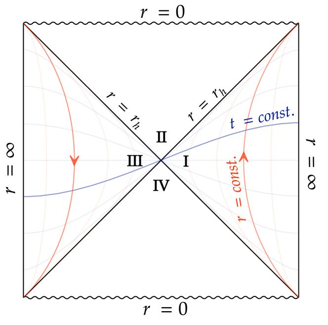
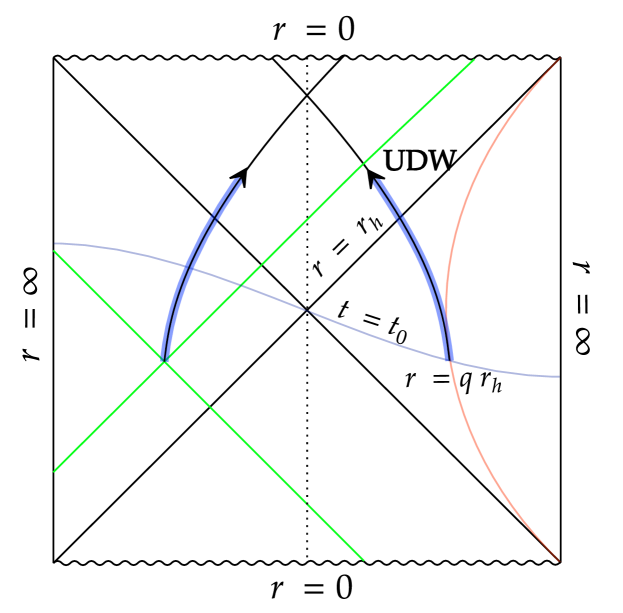
and the identification by (12) gives the extended spinless BTZ black-and-white hole spacetime. The Penrose-Carter diagram is shown in Figure 1. The exterior (5) is the region where and , wherein the coordinate transformation from to reads
| (13) |
The exterior timelike Killing vector extends to the whole BTZ black hole spacetime as , which is timelike in the two exteriors, spacelike in the black hole and white hole interiors, and null on the Killing horizons separating these four quadrants.
II.3 Geon spacetime
The geon black hole (or more simply geon) is obtained from the spinless BTZ spacetime by an identification under the map
| (14) |
Since on the BTZ spacetime, it is evident that , and therefore generates a action on the BTZ spacetime. Therefore, the geon spacetime is the quotient spacetime .
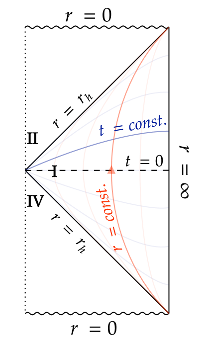
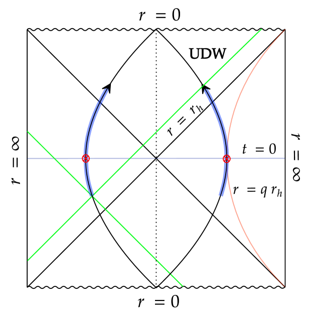
In the Penrose-Carter diagram of the BTZ spacetime, shown in Figure 1, (14) acts by a left-right reflection in the dimensions shown, composed with the antipodal map in the suppressed circle. It follows that the Penrose-Carter diagram of the geon consists of the (say) right half of the BTZ diagram, as shown in Figure 2. The geon is time orientable, and it has the nonorientable spatial topology .
As seen from Figure 2, the geon is an eternal black-and-white hole spacetime. It has a single exterior region, isometric to an exterior of the BTZ hole, and this region is static, with the timelike hypersurface-orthogonal Killing vector . Because of the unusual topology behind the horizons, however, does not extend to a globally-defined Killing vector on the whole geon spacetime: in Figure 2, the extension has a sign inconsistency at the vertical dotted line on the left. The topology behind the horizons therefore endows the exterior with a distinguished hypersurface of constant , shown in Figure 2 as : this is the only constant hypersurface that extends from the exterior smoothly to the horizon. The distinguished hypersurface cannot be identified by active classical observations in the exterior, and this exemplifies the topological censorship theorem [2, 3, 4]. The hypersurface can however be identified by quantum observations of a state that has been adapted to the geon’s global geometry, to which we now turn.
II.4 The Wightman function for the AdS, BTZ and geon spacetimes
We consider a detector interacting with a conformally coupled massless scalar field , that is, the field satisfies the Klein-Gordon equation , where is the d’Alembert operator and is the Ricci scalar.
In order to study the transition rate of a UDW detector, the Wightman function in the field’s initial state must be computed. For both the BTZ spacetime and the geon spacetime, we consider the initial state that is induced by the global vacuum on AdS3. As both the BTZ spacetime and the geon spacetime are quotients of an open region on AdS3 by a discrete isometry group, the strategy is to use the method of images.
Recall that the Wightman function in the global vacuum on AdS3 reads [35]
| (15) |
where
| (16) |
and the parameter specifies the boundary condition at the asymptotically AdS infinity. is the Dirichlet condition and is the Neumann condition, and both of these define a unitary quantum theory, with no probability entering or exiting through the infinity. is known as the transparent boundary condition, which classically allows probability to exit the spacetime through the infinity, and has a less clear physical interpretation in the quantum theory.
Note that (16) is half of the dimensionless squared geodesic distance in the embedding space (7) [9]; we shall henceforth refer to simply as the geodesic distance. Note also that has distributional singularities at the zeroes of the denominators in (15), and its full definition includes an prescription for these singularities and the branch points of the square roots. We shall address this shortly.
Now, the Wightman functions that induces on the BTZ spacetime and on the geon spacetime are, respectively [35, 36],
| (17a) | ||||
| (17b) | ||||
On the BTZ spacetime, has the characteristics of a Hartle-Hawking-Israel (HHI) vacuum [37, 38], describing a black hole in thermal equilibrium with a heat bath at infinity [35]. On the geon spacetime, is not a thermal equilibrium state as it is not invariant under the exterior Killing time translations, but it still has some characteristics of a HHI state [7, 11, 12, 39].
When the points and are in the exterior region, equations (8), (9), (14) and (16) give
| (18a) | ||||
| (18b) | ||||
where and , and the limit in (18a) specifies the distributional character of the Wightman function. Note that (18a) depends on and only via the combination , showing explicitly that is invariant under the exterior Killing time translations, but (18b) depends on and only via the combination , showing that is not invariant under the exterior Killing time translations.
II.5 Free-falling detector
Our interest is in computing, in different parameter regimes, the transition rate of a UDW detector that is radially free-falling into the geon and comparing it to its BTZ counterpart. We are particularly interested in the transition rate of the detector near and beyond the horizon.
In this scenario, the detector’s trajectory in the exterior region is given by [9]
| (19) | ||||
where is a dimensionless affine parameter, and , and are constants. is the value of the exterior Killing time at which reaches its maximum value. is the constant value of on the trajectory.
Inserting (19) into (18a) with and into (18b) with , we obtain
| (20a) | ||||
| (20b) | ||||
where
| (21a) | ||||
| (21b) | ||||
and
| (22a) | ||||
| (22b) | ||||
with . The constant does not appear, as must be the case by the invariance of the spacetimes and the quantum states under rotations in . The constant has disappeared from the expressions relevant for the BTZ spacetime, as must be by the invariance under the Killing time translations, but it remains in expressions relevant for the geon spacetime, which reflects the absence of global Killing time translations on the geon.
Using the above expressions, we find that the transition rate on the BTZ spacetime is given by
| (23) |
and that on the geon is given by
| (24) |
where
| (25) |
where , , and is the proper time at which the detector is switched on. The square roots in (23) and (25) are positive for positive arguments, and they are analytically continued to negative arguments by giving a small negative imaginary part, as follows from the distributional properties of the Wightman function [9, 25].
Although equations (18) are only valid exterior to the black hole, the transition rate formulas (23)–(25) hold also for detectors that operate even before exiting the white hole and/or after entering the black hole. This follows by analytic continuation, since both the BTZ hole and the geon have global analytic charts, as seen from (11).
III Analytic results
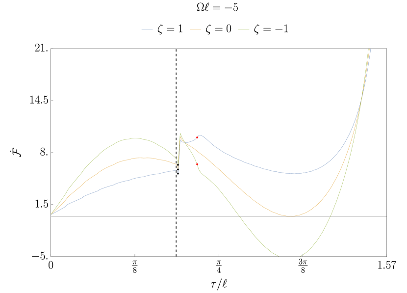
While both and are well defined, their derivatives with respect to have discontinuities at values of where a denominator in the integrand in (23) or (25) is singular at an endpoint of integration. We refer to these discontinuities in the derivative as ‘glitches’ [23]. In this section we present analytic estimates of where these glitches occur for the BTZ spacetime and for the geon spacetime.
III.1 BTZ glitches
Consider first the geodesic distance in BTZ spacetime.
For , , and only equals zero if the points at and are null-separated. This occurs in (23) at the lower limit of integration (=0), where the two points in fact coincide, and it does not introduce any singularities nor any need for analytic continuation.
The situation is different for because, physically, this represents the distance between a point on the trajectory and a point on an identical trajectory but translated by in AdS spacetime. Therefore, by choosing appropriately, it is always possible to find two points on the two trajectories that are null-separated if they are in causally connected regions of spacetime.
The argument of the square root in the -dependent term is positive for all in the interval and all . However in the first term, the argument of the square root can change of sign within the interval of integration for . This results in a singularity in the integrand, but the singularity is of the inverse square root type and hence integrable. Analytically solving the equation , we obtain
| (26) |
Examining , we find that for , for all . Since within the first integral in (23) the integration variable , there will be a time at which the singularity in the integrand coincides with the endpoint of the integration interval , given by the expression
| (27) |
which is equivalent to directly solving the equation:
| (28) |
Solving this analytically yields
| (29) |
These points are visible in the transition rate as points of non-differentiability; these are the ‘glitches’ noted above. However the transition rate remains well defined at these points.
In the case where , in which the detector is turned on at the moment when reaches its maximum value, the expression (29) simplifies to [23]
| (30) |
It is interesting to note that these glitches can be detected even before the detector crosses the event horizon. This follows from the fact that, if the parameters are such that , then , where is the instant at which the detector crosses the event horizon.
It is worth noting that the transition rate calculated with the term alone has a simplified expression, found in Eq. (6.5) of [9]. Also, the terms do not change under , so the transition rate can be written as twice the sum over .
III.2 Geon glitches
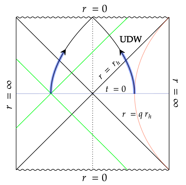
The transition rate associated with the geon black hole consists of two terms. One term is identical to the BTZ rate (23); the other is given by (25). This extra term is obtained from the BTZ rate (23) by substitution of (20b) in place of (20a). This means that the glitches present in the transition rate of a detector in the geon spacetime will be the same as those in the BTZ case, plus additional glitches specific to the geon, obtained by solving , or, for , also . Geometrically, the second case corresponds to a null geodesic that connects the switch-on event to a later event on the trajectory after reflection from infinity. In this section we consider only the first of these cases, but we shall return to the second case in Section IV.4. We note from (22b) that the sum in (25) is invariant under , so it suffices to sum over and double the result.
Where are these latter glitches located? In general, there are different cases depending on the value of the parameters and . This can be understood by analyzing the Penrose-Carter diagram of the BTZ black hole; in this spacetime, (20b) represents the distance between a point on the detector’s trajectory and a point on its mirror image with a shift in by . Geon glitches occur when a null ray from the image detector emitted at proper time intersects the trajectory of the original detector in the geon covering space. We can qualitatively predict what happens to the geon glitches for different values of and , keeping in mind that in the Penrose-Carter diagram the coordinate is suppressed, so what we can draw are the null rays that travel radially. In this analysis the intersection between the null ray and the detector’s trajectory does not give us the exact position of the glitches, but does give a bound as to where the geon glitches can or cannot occur; the actual null rays have to travel through the direction by an odd multiple of . This approach gives us a good protocol for gaining insight into the transition rate without relying on analytical expressions for the glitches. Additionally, it serves as a consistency check for our numerical results.
We consider in turn the case where , the case where , and the case where . The features of the generic case, in which , can be inferred from these.
III.2.1
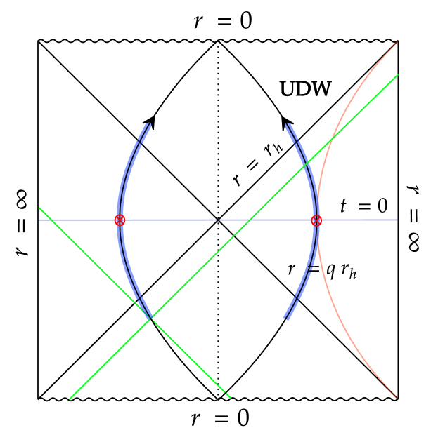
Consider first the case in which . As illustrated in Figure 3, changing the value of generates the three distinct scenarios described below.
-
•
: From the top diagram in Figure 3, we observe that a null ray from the initial location of the image detector (at the left) encounters the trajectory of the original detector (at the right), so it is possible to detect glitches in this regime, albeit only inside the horizon as shown in the diagram.
-
•
: From the middle diagram in Figure 3, we observe that geon glitches can be observed from within the horizon. However the first geon glitch occurs closer to the future singularity than in the case. By continuity there is a time such that no geon glitches will be observable before the detector encounters the singularity.
-
•
: From the bottom diagram in Figure 3, we see that null rays from the image detector at the left can reach the original infalling detector before either encounters the singularity. Multiple geon glitches can therefore occur, but all of them will be behind the event horizon. Moreover, we expect that .
It is easy to find the position of the geon glitches in analytic form. Following the same definition adopted for the BTZ case, we obtain
| (31) |
with . It can be easily seen that
| (32a) | ||||
| (32b) | ||||
By analyzing (31) it is evident that there are also solutions for and that the position of the glitches grows with . As increases, eventually the argument of the arccos in (31) is equal to zero, at ; for larger values of the glitches reach the singularity before they can be detected along the trajectory. As we can infer from the middle diagram in Figure 3, as increases, the location at which the detector encounters the singularity moves increasingly rightward, and no more glitches can occur for , where
| (33) |
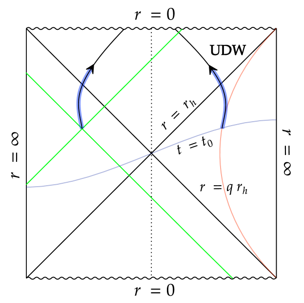
III.2.2
Consider next the case in which . The geodesic distance (20b) becomes
| (34) |
with . This expression is identical to (20a), with the substitution of the function (22b) in place of (22a). Hence, the positions of “geon glitches” are
| (35) |
The argument of the arccos in (35) is always greater than zero, so geon glitches are always detectable throughout the trajectory, with
| (36a) | ||||
| (36b) | ||||
The effect of changing is shown in the Penrose-Carter diagrams in Figure 4. The key new feature is that when , so that the detector operates already before emerging from the white hole region, glitches can occur already before the detector enters the black hole region.
III.2.3
Consider finally the case in which . Equation (35) assumes now the simple form
| (37) |
Since , we have , for all . It follows that the distinct topologies of the two black holes, in terms of their signature glitches, only become evident after crossing the horizon.
IV Numerical results
In this section, we present results from numerical calculations of the transition rate of a detector in each spacetime. Subsection IV.1 addresses the special case , in which case the detector is switched on at the moment of maximum radius on the trajectory, and, on the geon, this moment is at the distinguished hypersurface. Subsections IV.2 and IV.3 address respectively the cases where and . The features present in the generic case, , can be deduced from these.
To ensure convergence of the numerics, the number of terms used was calculated so that the first neglected term in the sums (23), (25) for every was less than .
IV.1
Consider first the case , shown in Figure 3 top panel.
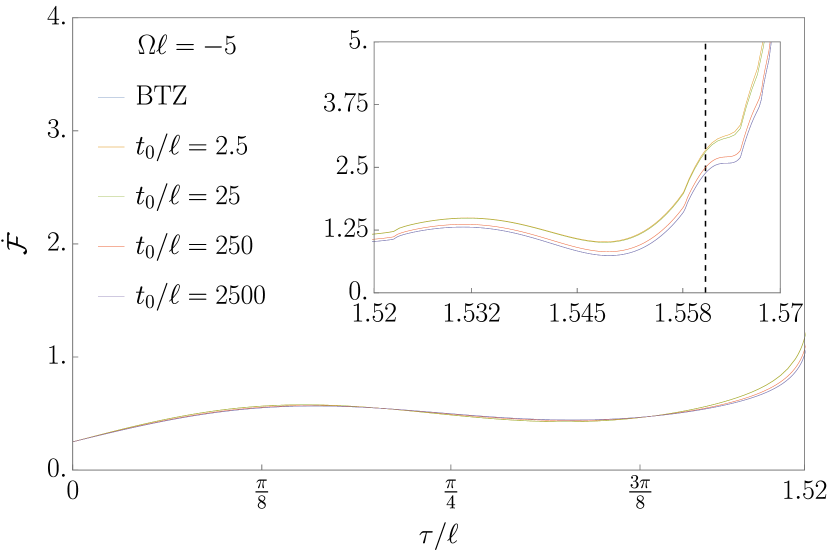
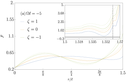
Figure 5 shows the transition rate as a function of for and , for selected values of . The difference between the BTZ spacetime and the geon spacetime grows as the mass decreases, with the amplitude on the geon being larger. For both, the oscillations increase in both frequency and amplitude further from the horizon as the mass decreases.
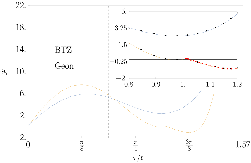
Figure 6 shows the transition rate as a function of for a detector released much closer to the horizon, at , for . The first geon glitch is clearly discernible in the plot, behind the horizon at , by (37) with .
Figure 7 shows the transition rate as a function of for a range of positive and negative energy gaps and a range of masses. As with Figure 6, it is immediately noticeable that the geon and BTZ curves are not identical even before crossing the horizon. In both cases the rate exhibits quasi-oscillations outside the horizon of approximately the same frequency, but with the amplitude of the geon rate being slightly larger. The oscillation frequency decreases with decreasing gap magnitude and increasing mass, as already seen in Figure 5.
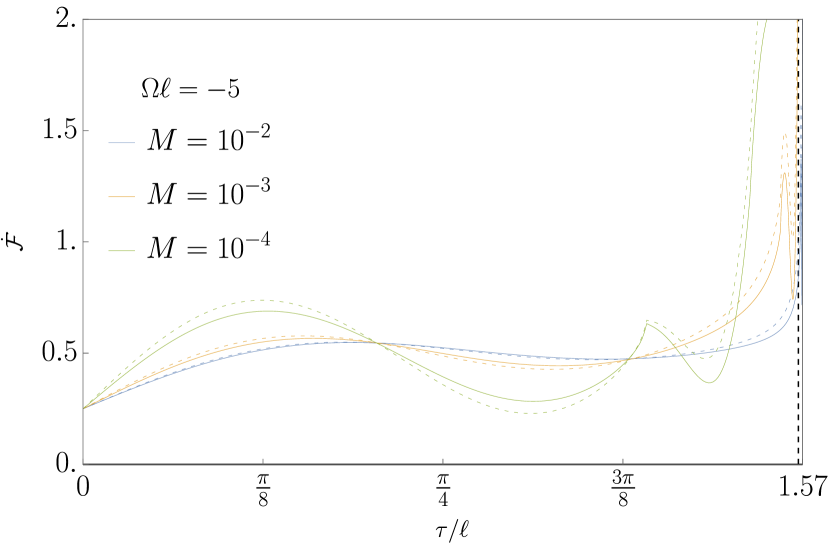
This trend persists until the first glitch, after which the geon transition rate grows more rapidly than the BTZ rate as the detector approaches the singularity, for both signs of . Outside the horizon, the glitches agree for the two spacetimes, at the positions determined by (30), as is clearly visible in the upper diagrams where . The geon glitches occur only beyond the horizon and are easily visible for the small value of in Figure 6. They are not easily visible in Figure 7, where the large value of implies that these glitches are close to the singularity , where .
The transition rate is relatively insensitive to the value of the energy gap beyond the first glitch. The effect of the gap is mainly observed in the BTZ case (23), where for positive gaps there are oscillations after the first glitch that increase with [23]. For negative gaps, the trend remains monotonically increasing, interspersed with glitches.
What seems to particularly influence the transition rate is the mass . As the mass increases, two effects are observed: the glitches move to the right, and there is a noticeable decrease in . This effect can be easily observed by examining the expressions (17), where it is clear from (18) that for , the only surviving term is the zeroth-order term of (17a). The cause of this effect is the dependence of and on . However, since for fixed , , and , the terms in the sum related to the geon are suppressed more rapidly.
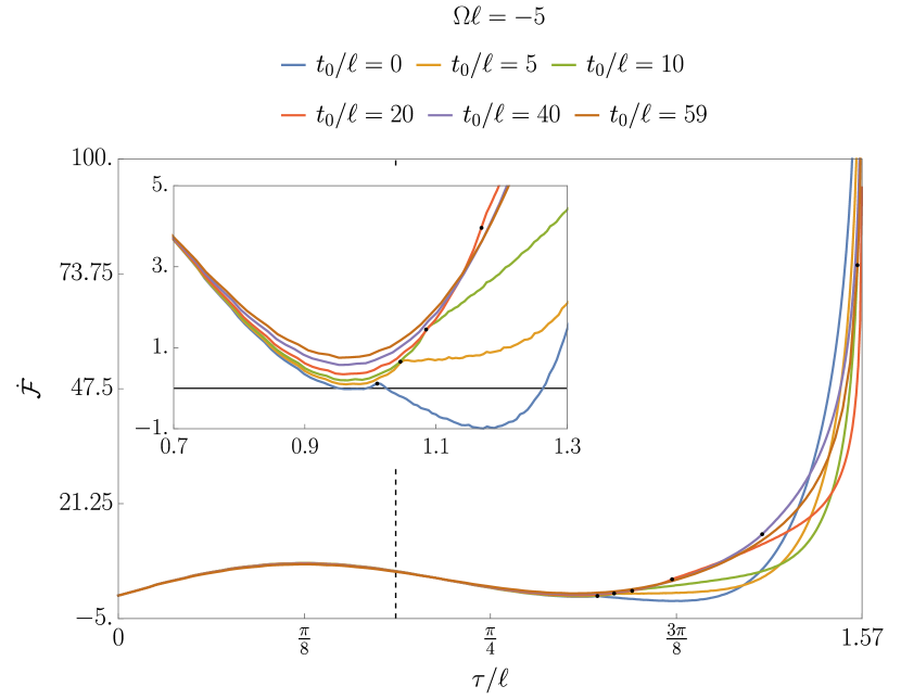
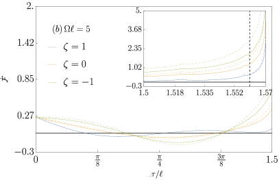
IV.2
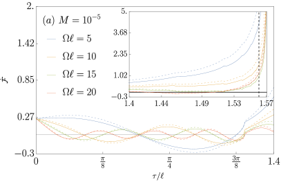
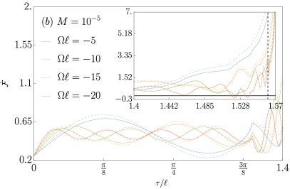
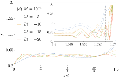
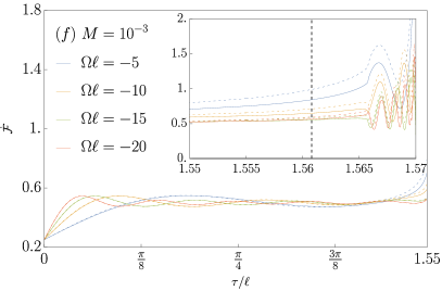
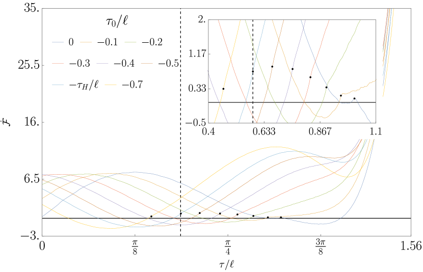
Consider next the case , shown in Figure 3 middle and bottom panels. As discussed in Section III, the value of does not affect the transition rate on the BTZ spacetime, but it does affect the transition rate on the geon.
Figure 8 shows the transition rate on the BTZ spacetime and the geon spacetime with three different negative values of and various values of , the other parameters being , and . The differences between the BTZ transition rate and the geon transition rate again become significant only when the detector is close to the horizon, and when is large and negative, this happens very close to the horizon-crossing moment in the detector’s proper time, because the detector then spends little proper time between the distinguished Killing time surface and the horizon, as is seen from the bottom panel in Figure 3. The jitter persisting after the first glitch is caused by the subsequent glitches.
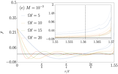
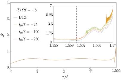
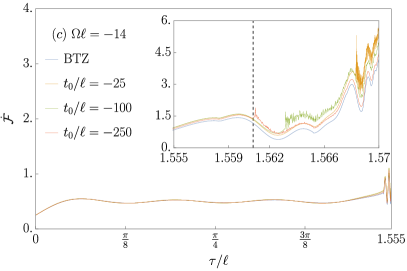
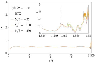
Figures 10 and 9 shows the transition rate on the geon spacetime for various positive values of and selected values of the other parameters. The glitch structure behind the horizon is now suppressed for large positive , as was to be expected from the middle panel in Figure 3.
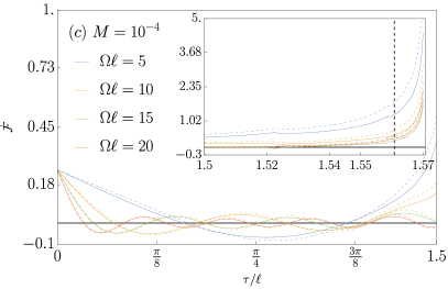
IV.3
Consider finally the case .
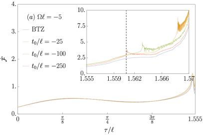
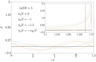
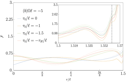
We consider only the case , in which the detector starts to operate before reaching the maximum value of on the distinguished hypersurface. This is the spacetime diagram in Figure 4. Numerical results are shown in Figures 11 and 12.
The figures show that glitches move towards earlier proper times as becomes more negative. Glitches before crossing the black hole horizon can occur only when , so that the detector has started to operate before emerging from the white hole part of the spacetime, as shown in Figure 4 lower panel: one such glitch is seen for one of the trajectories in Figure 11.
IV.4
We now comment on what differs for the Dirichlet and Neumann boundary conditions, .
Over most of the parameter space, we find that the response is qualitatively similar to the response. A sample plot for is shown in Figure 13.
However, there are regions of the parameter space where the term introduces new glitches in the response. Geometrically, these new glitches come from null geodesics that connect the switch-on moment to a later moment on the trajectory by reflection from infinity. Consideration of Figure 3 lower panel shows that one situation where this happens is for when is sufficiently negative, and the new glitches then occur after the detector has entered the black hole. Analytically, the new glitches come by solving , which yields a new set of glitches positioned at
| (38) |
where the superscript ‘b’ denotes that these glitches originate from the term in (25). These glitches exist for , where
| (39) |
All of these glitches occur after the detector has crossed the future horizon, and as , they occur shortly after the horizon-crossing,
| (40) |
For high values of , these glitches are not easily visually distinguishable from the glitches, but Figure 14 shows a plot where they are distinguishable for .
V Conclusions
We have computed and compared the transition rates of a radially infalling Unruh-DeWitt detector into a BTZ black hole and the geon, the latter being obtained from the former by a topological identification. The geon topology is hidden behind its horizon, and so the two spacetimes are classically indistinguishable outside the horizon.
Our results are commensurate with previous work on static detector response and entanglement in geon spacetimes [8, 40, 15], but reveal additional features. The pointwise difference between the two rates is indeed different from zero even outside the black hole, as for the static case [8]. Glitches observed in the BTZ case [23] occur in identical places for the geon outside of the horizon. However there are extra glitches associated with the geon, representing a significant difference between the two rates. Assuming that the detector’s interaction with the field begins when the detector is in the black hole exterior, these extra glitches occur only after the detector has entered the black hole. This result is consistent with the topological censorship theorem [2] and with what one would expect from classical considerations.
Nevertheless, the infalling detector can probe interior topology prior to encountering the horizon insofar as the amplitude of the geon response rate is larger than that of its BTZ counterpart. While less dramatic than the signature glitches inside the horizon, it is significant that an infalling quantum detector is sensitive to hidden topology.
Acknowledgements
We thank Chris Shallue and Sean Carroll for sharing with us an early copy of their work on the Schwarzschild infall [18]. This work was supported in part by the Natural Sciences and Engineering Research Council of Canada. MRPR gratefully acknowledges the support provided by the Mike and Ophelia Lazaridis Graduate Fellowship. The work of JL was supported by United Kingdom Research and Innovation Science and Technology Facilities Council [grant numbers ST/S002227/1, ST/T006900/1 and ST/Y004523/1]. For the purpose of open access, the authors have applied a CC BY public copyright licence to any Author Accepted Manuscript version arising.
References
- Penrose [1999] R. Penrose, The question of cosmic censorship, Journal of Astrophysics and Astronomy 20, 233 (1999).
- Friedman et al. [1995] J. L. Friedman, K. Schleich, and D. M. Witt, Topological Censorship[Phys. Rev. Lett. 71, 1486 (1993)], Physical Review Letters 75, 1872–1872 (1995).
- Galloway and Woolgar [1997] G. Galloway and E. Woolgar, The Cosmic censor forbids naked topology, Classical and Quantum Gravity 14, L1 (1997), arXiv:gr-qc/9609007 .
- Galloway et al. [1999] G. J. Galloway, K. Schleich, D. M. Witt, and E. Woolgar, Topological censorship and higher genus black holes, Physical Review D 60, 104039 (1999), arXiv:gr-qc/9902061 .
- Unruh [1976] W. G. Unruh, Notes on black-hole evaporation, Physical Review D 14, 870 (1976).
- DeWitt [1979] B. S. DeWitt, Quantum gravity: The new synthesis, in General Relativity: An Einstein Centenary Survey, edited by S. W. Hawking and W. Israel (Cambridge University Press, Cambridge, England, 1979) pp. 680–745.
- Louko and Marolf [1998] J. Louko and D. Marolf, Inextendible Schwarzschild black hole with a single exterior: How thermal is the Hawking radiation?, Physical Review D 58, 024007 (1998), arXiv:gr-qc/9802068 .
- Smith and Mann [2014] A. R. H. Smith and R. B. Mann, Looking inside a black hole, Classical and Quantum Gravity 31, 082001 (2014).
- Hodgkinson and Louko [2012] L. Hodgkinson and J. Louko, Static, stationary and inertial Unruh-DeWitt detectors on the BTZ black hole, Physical Review D 86, 064031 (2012), arXiv:1206.2055 [gr-qc] .
- Hodgkinson et al. [2014] L. Hodgkinson, J. Louko, and A. C. Ottewill, Static detectors and circular-geodesic detectors on the Schwarzschild black hole, Physical Review D 89, 104002 (2014), arXiv:1401.2667 [gr-qc] .
- Louko and Marolf [1999] J. Louko and D. Marolf, Single exterior black holes and the AdS / CFT conjecture, Physical Review D 59, 066002 (1999), arXiv:hep-th/9808081 .
- Louko et al. [2000] J. Louko, D. Marolf, and S. F. Ross, On geodesic propagators and black hole holography, Physical Review D 62, 044041 (2000), arXiv:hep-th/0002111 .
- Galloway et al. [2001] G. J. Galloway, K. Schleich, D. Witt, and E. Woolgar, The AdS / CFT correspondence conjecture and topological censorship, Physics Letters B 505, 255 (2001), arXiv:hep-th/9912119 .
- Martín-Martínez et al. [2016] E. Martín-Martínez, A. R. H. Smith, and D. R. Terno, Spacetime structure and vacuum entanglement, Physical Review D 93, 044001 (2016), arXiv:1507.02688 [quant-ph] .
- Henderson et al. [2022] L. J. Henderson, S. Y. Ding, and R. B. Mann, Entanglement harvesting with a twist, AVS Quantum Science 4, 014402 (2022), arXiv:2201.11130 [quant-ph] .
- Ahmadzadegan et al. [2014] A. Ahmadzadegan, E. Martín-Martínez, and R. B. Mann, Cavities in curved spacetimes: the response of particle detectors, Physical Review D 89, 024013 (2014), arXiv:1310.5097 [quant-ph] .
- Ng et al. [2022] K. K. Ng, C. Zhang, J. Louko, and R. B. Mann, A little excitement across the horizon, New Journal of Physics 24, 103018 (2022).
- [18] C. J. Shallue and S. M. Carroll, private communication (2024).
- Juárez-Aubry and Louko [2014] B. A. Juárez-Aubry and J. Louko, Onset and decay of the 1+1 Hawking-Unruh effect: What the derivative-coupling detector saw, Classical and Quantum Gravity 31, 245007 (2014).
- Juárez-Aubry [2016] B. A. Juárez-Aubry, Asymptotics in the time-dependent Hawking and Unruh effects, PhD thesis, University of Nottingham (2016), available at https://eprints.nottingham.ac.uk/id/eprint/32924.
- Gallock-Yoshimura et al. [2021] K. Gallock-Yoshimura, E. Tjoa, and R. B. Mann, Harvesting entanglement with detectors freely falling into a black hole, Physical Review D 104, 025001 (2021), arXiv:2102.09573 [quant-ph] .
- Juárez-Aubry and Louko [2022] B. A. Juárez-Aubry and J. Louko, Quantum kicks near a Cauchy horizon, AVS Quantum Science 4 (2022).
- Preciado-Rivas et al. [2024] M. R. Preciado-Rivas, M. Naeem, R. B. Mann, and J. Louko, More excitement across the horizon, Physical Review D 110, 025002 (2024), arXiv:2402.14908 [gr-qc] .
- Wang et al. [2024] S. Wang, M. R. Preciado-Rivas, M. Spadafora, and R. B. Mann, Singular excitement beyond the horizon of a rotating black hole, Physical Review D 110, 065013 (2024), arXiv:2407.01673 [gr-qc] .
- Kay and Wald [1991] B. S. Kay and R. M. Wald, Theorems on the Uniqueness and Thermal Properties of Stationary, Nonsingular, Quasifree States on Space-Times with a Bifurcate Killing Horizon, Physics Reports 207, 49 (1991).
- Fewster [2000] C. J. Fewster, A General worldline quantum inequality, Classical and Quantum Gravity 17, 1897 (2000), arXiv:gr-qc/9910060 .
- Junker and Schrohe [2002] W. Junker and E. Schrohe, Adiabatic vacuum states on general space-time manifolds: Definition, construction, and physical properties, Annales Henri Poincaré 3, 1113 (2002), arXiv:math-ph/0109010 .
- Louko and Satz [2008] J. Louko and A. Satz, Transition rate of the Unruh-DeWitt detector in curved spacetime, Classical and Quantum Gravity 25, 055012 (2008), arXiv:0710.5671 [gr-qc] .
- Langlois [2005] P. Langlois, Imprints of spacetime topology in the Hawking-Unruh effect, Ph.D. thesis, University of Nottingham (2005), arXiv:gr-qc/0510127 .
- Satz [2007] A. Satz, Then again, how often does the Unruh-DeWitt detector click if we switch it carefully?, Classical and Quantum Gravity 24, 1719 (2007), arXiv:gr-qc/0611067 .
- Bañados et al. [1992] M. Bañados, C. Teitelboim, and J. Zanelli, Black hole in three-dimensional spacetime, Physical Review Letters 69, 1849 (1992).
- Bañados et al. [1993] M. Bañados, M. Henneaux, C. Teitelboim, and J. Zanelli, Geometry of the 2+1 black hole, Physical Review D 48, 1506 (1993).
- Jennings [2010] D. Jennings, On the response of a particle detector in Anti-de Sitter spacetime, Classical and Quantum Gravity 27, 205005 (2010), arXiv:1008.2165 [gr-qc] .
- Henderson et al. [2020] L. J. Henderson, R. A. Hennigar, R. B. Mann, A. R. H. Smith, and J. Zhang, Anti-Hawking phenomena, Physics Letters B 809, 135732 (2020), arXiv:1911.02977 [gr-qc] .
- Lifschytz and Ortiz [1994] G. Lifschytz and M. Ortiz, Scalar field quantization on the (2+1)-dimensional black hole background, Physical Review D 49, 1929–1943 (1994).
- Carlip [1995] S. Carlip, The (2+1)-dimensional black hole, Classical and Quantum Gravity 12, 2853 (1995).
- Hartle and Hawking [1976] J. B. Hartle and S. W. Hawking, Path Integral Derivation of Black Hole Radiance, Physical Review D 13, 2188 (1976).
- Israel [1976] W. Israel, Thermo field dynamics of black holes, Physics Letters A 57, 107 (1976).
- Guica and Ross [2015] M. Guica and S. F. Ross, Behind the geon horizon, Classical and Quantum Gravity 32, 055014 (2015), arXiv:1412.1084 [hep-th] .
- Smith [2019] A. R. H. Smith, Detectors, reference frames, and time, Springer Theses https://doi.org/10.1007/978-3-030-11000-0 (2019).