From dynamical to steady-state many-body metrology:
Precision limits and their attainability with two-body interactions

Abstract

We consider the estimation of an unknown parameter $\theta$ via a many-body probe. The probe is initially prepared in a product state and many-body interactions enhance its $\theta$-sensitivity during the dynamics and/or in the steady state. We present bounds on the Quantum Fisher Information, and corresponding optimal interacting Hamiltonians, for two paradigmatic scenarios for encoding $\theta$: (i) via unitary Hamiltonian dynamics (dynamical metrology), and (ii) in the Gibbs and diagonal ensembles (time-averaged dephased state), two ubiquitous steady states of many-body open dynamics. We then move to the specific problem of estimating the strength of a magnetic field via interacting spins and derive two-body interacting Hamiltonians that can approach the fundamental precision bounds. In this case, we additionally analyze the transient regime leading to the steady states and characterize tradeoffs between equilibration times and measurement precision. Overall, our results provide a comprehensive picture of the potential of many-body control in quantum sensing.

I Introduction

Quantum Metrology is concerned with the precise estimation of physical quantities which can range from the strength of a magnetic field to the temperature of ultra-cold gases, beyond the capability of conventional classical sensors by exploiting quantum resources such as quantum coherence or entanglement [1, 2]. A central problem in quantum metrology is the estimation of a parameter $\theta$ of a Hamiltonian $H_{\theta}$. For time-independent $H_{\theta}$, this can typically be expressed as

$$H_{\theta}=\theta H_{S}+H_{C}\,.$$ (1)

Here, $H_{S}$ is the part of the Hamiltonian encoding the signal, whereas $H_{C}$ includes any other contribution. The latter can range from the action of an uncontrolled environment to a control term designed to enhance the measurement precision. Considering a quantum state $\rho_{0}$ evolving under $U=\exp(-itH_{\theta})$, where we set $\hbar=1$, the Cramér-Rao bound tells us that the uncertainty $\Delta\theta$ is bounded as [3]

$$(\Delta\theta)^{2}\geq\frac{1}{\mu\,t^{2}\|H_{S}\|^{2}}\,,$$ (2)

where $\mu$ is the number of measurements, and we defined the pseudo-norm $\|H_{S}\|=\lambda_{\rm max}^{S}-\lambda_{\rm min}^{S}$ with $\lambda_{\rm max}^{S}$ ($\lambda_{\rm min}^{S}$) the maximal (minimal) eigenvalue of $H_{S}$. For example, in magnetometry with $N$ spins, $H_{S}=\frac{1}{2}\sum_{j=1}^{N}\sigma_{z}^{(j)}$, we recover the standard (dynamical) Heisenberg limit $(\Delta\theta)^{-2}\leq\mu t^{2}N^{2}$. This can be contrasted to the standard shot-noise limit (SNL) $\mu Nt^{2}$ obtained for independent coherently evolving systems [1, 2].

	Dynamical with	Steady state:	Steady state:
	initial ground state of $H_{S}$	Diagonal ensemble	Gibbs ensemble
General upper bound	$\mathcal{F}\leq t^{2}\|H_{S}\|^{2}$    (Ref. [3])	$\mathcal{F}\leq\frac{3+\pi^{2}}{3}\frac{\|H_{S}\|^{2}}{E^{2}}$   (Result 5)	$\mathcal{F}\leq\frac{1}{4}\beta^{2}\|H_{S}\|^{2}$   (Ref. [4])
Best known protocol with unrestricted $H_{C}$	$\mathcal{F}\approx\frac{1}{4}t^{2}\|H_{S}\|^{2}$   (Result 2)	$\mathcal{F}=\frac{3}{2}\frac{\|H_{S}\|^{2}}{E^{2}}$       (Result 6)	$\mathcal{F}=\frac{1}{4}\beta^{2}\|H_{S}\|^{2}$   (Ref. [4])

Table 1: Summary of main results for arbitrary encoding $H_{S}$. All upper bounds depend on $||H_{S}||=\lambda_{\rm max}^{S}-\lambda_{\rm min}^{S}$ with $\lambda_{\rm max}^{S}$ ($\lambda_{\rm min}^{S}$) the maximal (minimal) eigenvalue of $H_{S}$. Up to constants, the time $t$ is replaced by $\beta$ for Gibbs state metrology and by $E^{-2}$ for the diagonal ensemble with $E$ the minimal non-zero energy gap of $H_{\theta}$ (we choose units in which $\hbar=1$). All upper bounds can be saturated, up to constants, by explicit Hamiltonian control $H_{C}$, see details below.

	Dynamical with	Steady state:	Steady state:
	initial product state	Diagonal ensemble	Gibbs ensemble
Bound for $N$-spin probe ($\|H_{S}\|=N$)	$\mathcal{F}\leq t^{2}N^{2}$	$\mathcal{F}\leq\frac{3+\pi^{2}}{3}\frac{N^{2}}{E^{2}}$	$\mathcal{F}\leq\frac{1}{4}\beta^{2}N^{2}$
Best-known protocol with two-body $H_{C}$	$\mathcal{F}\approx\frac{1}{4}t^{2}N^{2}$   (Result 3)	$\mathcal{F}\approx\frac{1.34N^{3/2}}{E^{2}}$   (Result 7)	$\mathcal{F}\approx\frac{1}{4}\beta^{2}N^{2}$   (Result 9)

Table 2: Summary of main results for sensing a magnetic field with a $N$-spin interacting probe. In this work, we show that a central spin model can approach the Heisenberg limit (up to a $1/4$ factor). We also show numerically that with a collective spin coupling as in Eq. (4) we can achieve a comparable performance. With a suitable choice of interaction strengths, this model can also saturate the QFI bound for the Gibbs ensemble and achieve a $N^{3/2}$ scaling for the QFI of the diagonal ensemble.

The most common approach to overcome the SNL consists of preparing $\rho_{0}$ as a carefully entangled state, which requires a prior preparation stage, while assuming $H_{C}=0$ [1, 2]. Yet, recent years have witnessed an increased interest in understanding the potential of many-body interactions, i.e. taking $H_{C}\neq 0$ and $\rho_{0}$ as a product state, for overcoming the SNL and achieving enhanced metrology [5, 6, 7]. Within the study of quantum metrology with many-body systems, we distinguish two main scenarios: dynamical and static (or steady-state).

The dynamical scenario corresponds to the situation described above in which information on $\theta$ is encoded into the many-body probe through unitary evolution under $H_{\theta}$, and both time $t$ and the number of particles $N$ are accounted as resources. By properly engineering $H_{\theta}$ close to a dynamical phase transition, it is possible for the measurement sensitivity $\mathcal{F}$ to scale beyond the SNL [6, 8, 9]. This has been shown for the Lipkin-Meshkov-Glick (LMG) model obtaining up to $\mathcal{F}\sim t^{2}N^{1.75}$ [10] as well as more general long-range Ising models [11]; see also results for stark localized systems [12, 13], fermionic lattices [14] and quantum-optics systems [15, 9, 16, 17, 18, 19, 20]. Using the Lieb-Robinson bound, it has been recently shown that long-range interactions are required to beat the SNL when starting from a product state [11, 21].

In the static scenario, information on $\theta$ is instead encoded in the steady state of the system, which may be a ground, thermal, or non-equilibrium steady state. This can be connected to the dynamical approach by assuming the presence of an environment and taking the limit $t\rightarrow\infty$ of the dissipative evolution. In this approach, time is not considered as a resource but only the number of particles $N$ is. As in the dynamical scenario, by exploiting phase transitions in the steady state, one can obtain a measurement sensitivity that scales beyond linear [22, 23, 24]. It is in principle possible to obtain scalings beyond $N^{2}$, but this comes at the expense of a diverging preparation time so that the general bound (2) is always respected for any (dissipative) dynamics [24, 25]. Within the static approach, numerous works have shown enhancements in the sensitivity of many body probes close to a critical point, either of ground [26, 27, 28, 5, 29], thermal [30, 26, 31, 32, 33, 34, 35, 36] or non-equilibrium steady states [37, 38, 39, 40, 41, 42].

Despite this relevant progress, a general understanding of the limits and potential of many-body quantum metrology is far from complete, both in the dynamic and static scenarios. Relevant questions include:

• Can we approach the fundamental dynamical bound in Eq. (2), starting from product states, via physically relevant $H_{C}$ (e.g. limited to two-body interactions)?

• Can we derive bounds similar to Eq. (2) but applicable instead to steady-state metrology?

The main goal of this work is to investigate such questions for closed and open systems. For that, we derive bounds for the Quantum Fisher Information (QFI) [43], which sets an ultimate limit on the measurement precision, and investigates their saturability. We consider time-independent $H_{\theta}$ and follow a twofold approach.

On the one hand, we characterize the QFI given a generic signal $H_{S}$ and arbitrary Hamiltonian control $H_{C}$. For dynamical metrology, we take as an initial state an eigenstate of $H_{S}$; this covers relevant cases as initial product states when $H_{S}$ is a sum of local terms and the ground state of $H_{S}$. Given a $H_{S}$, we then derive a $H_{C}$ that approaches the bound in Eq. (2) up to a constant $1/4$, which we believe to be optimal. For open systems, we derive a new bound on the QFI applicable to the long time-averaged state or diagonal ensemble [44, 45, 46, 47]. Together with the recent upper bound for the QFI of the Gibbs ensemble [4], these bounds can be seen as the counterpart of the one in Eq. (2) for relevant cases of steady state metrology ($t\rightarrow\infty$). We also develop optimal $H_{C}$ that can saturate these bounds. Our results for generic $H_{S}$ are summarized in Table 1.

On the other hand, we consider the particular case of magnetometry via a many-body spin probe, i.e.

$$H_{S}=S_{z}\,,$$ (3)

with $S_{j}=\frac{1}{2}\sum_{i=1}^{N}\sigma_{j}^{(i)}$ and $j=x,y,z$. We then look for the control Hamiltonian $H_{C}$ featuring only two-body interactions that can approach the upper bounds on the QFI (for dynamic and static metrology). In the case of closed systems, we analytically show that a central spin model can reach the scaling $N^{2}t^{2}$, but with a worse prefactor of $1/4$ when compared to the fundamental bound in Eq. (2). Beyond the central spin model, we focus on spin squeezing control Hamiltonians with two-body couplings of the form

$$H_{C}=aS_{x}^{2}+bS_{y}^{2}+cS_{z}^{2}\,.$$ (4)

This model involving collective spin variables is very natural in atomic ensembles used in magnetometry and interferometry [48, 49, 50, 51]. By appropriate choice of the $(a,b,c)$ coefficients, we numerically show that a Heisenberg scaling can be obtained in dynamical metrology (as for the central spin model). We also show that the control in Eq. (4) enables the saturation of the QFI bound for Gibbs states. For the diagonal ensemble, we find a scaling $N^{3/2}$ of the QFI for an appropriate choice of $(a,b,c)$. Our main results for magnetometry are summarized in Table 2.

Finally, in the same spin-probe scenario we study the transient regime to steady states. That is, we introduce appropriate noise models (corresponding to dephasing and thermalization) and evaluate the value of the QFI at all intermediate times leading to equilibration. We find again strong improvements attainable via many-body interactions, and we analyze the different tradeoffs between the scaling of equilibration time and QFI.

The paper is structured as follows. In Sec. II, we introduce the main quantities of interest. In Sec. III, we focus on closed systems and discuss various choices of $H_{C}$ while contrasting them to the bound in Eq. (2). In Sec. IV, we focus on steady-state metrology of the diagonal and Gibbs ensemble, by deriving both bounds on the QFI and strategies to approach them. In Sec. V, we build connections between both previous scenarios, by analyzing the finite-time performance of $H_{C}$ that becomes optimal in the steady state regime. Finally, we conclude in Sec. VI.

II framework

To estimate an unknown scalar parameter $\theta$, we consider an estimator $\hat{\theta}$. This estimator is a random variable dependent on the measurement results $\bm{x}$ sampled from $p(\bm{x}|\theta)$. The precision of an estimator can be quantified by its mean squared error, which is the expected square deviation of the estimator from the true value of the parameter.

Remarkably, the mean squared error of any locally unbiased estimator can be lower bounded with the Cramér-Rao Bound [52]

$$(\Delta\theta)^{2}\geq\frac{1}{\mu\,\mathcal{I}}\,,$$ (5)

where $\mu$ is the number of repetitions of the measurements and $\mathcal{I}=\mathds{E}\left[\partial_{\theta}\log p(\bm{x}|\theta)\right]$ is the Classical Fisher Information (CFI), which only depends on the outcome distribution $p(\bm{x}|\theta)$ and its derivative $\partial_{\theta}p(\bm{x}|\theta)$ at $\theta$. In addition, this inequality can be saturated asymptotically [53]. The CFI is thus a natural, estimator-independent, figure of merit to benchmark sensing strategies.

In a quantum framework, the probability distribution $p(\bm{x}|\theta)$ arises by measuring a quantum state $\rho_{\theta}$, which encodes information on $\theta$. Assuming that the optimal measurement is performed, we can substitute the CFI with its quantum version: the Quantum Fisher Information (QFI) $\mathcal{F}$. The QFI can be expressed in terms of the probe state evolved under the parameter-dependent dynamical process $\rho_{\theta}$ and its derivative with respect to the unknown parameter $\dot{\rho}_{\theta}=\partial_{\theta}\rho_{\theta}$. In its most general form, the QFI is

$$\mathcal{F} =\Tr[\mathds{J}^{-1}_{\rho_{\theta}}(\dot{\rho}_{\theta})\dot{\rho}_{\theta}]\,,$$ (6)

where we have defined $\mathds{J}^{-1}_{\rho_{\theta}}(\dot{\rho}_{\theta})$, to be the solution of the Lyapunov equation

$$\dot{\rho}_{\theta}=\frac{1}{2}\left[\mathds{J}^{-1}_{\rho_{\theta}}(\dot{\rho}_{\theta})\rho_{\theta}+\rho_{\theta}\mathds{J}^{-1}_{\rho_{\theta}}(\dot{\rho}_{\theta})\right]\,,$$ (7)

i.e. it is given by the inverse of the Bures multiplication super-operator $\mathds{J}_{\rho_{\theta}}[A]=\frac{1}{2}(A\rho_{\theta}+\rho_{\theta}A)$ applied on $\dot{\rho}_{\theta}$. Note that $\mathds{J}^{-1}_{\rho_{\theta}}(\dot{\rho}_{\theta})$ is equivalent to the Symmetric Logarithmic Derivative [43]. Under some constraints, the form of the QFI is simplified. Particularly, when we have a pure state, $\rho_{\theta}=\outerproduct{\psi_{\theta}}{\psi_{\theta}}$, the QFI is given by

$$\mathcal{F}=4\left(\innerproduct{\dot{\psi}_{\theta}}{\dot{\psi}_{\theta}}-\left|\innerproduct{\dot{\psi}_{\theta}}{{\psi}_{\theta}}\right|^{2}\right)\,,$$ (8)

where $\ket{\dot{\psi}_{\theta}}=\partial_{\theta}\ket{\psi_{\theta}}$.

Information on $\theta$ is encoded on $\rho_{\theta}$ via some dynamical process driven by the Hamiltonian $H_{\theta}$ given in Eq. (1). Importantly, in this work we assume that the $H_{\theta}$ can be split into two contributions (see Fig. 1):

• $H_{S}$: This corresponds to the signal, i.e., the part of $H_{\theta}$ encoding the unknown parameter $\theta$. We assume no control on $H_{S}$.

• $H_{C}$: This accounts for any other contribution which is $\theta$-independent. We will assume (partial) control on $H_{C}$ to enhance the sensitivity $\mathcal{F}_{\theta}$. We focus on time-independent $H_{C}$. Note that in principle $H_{C}$ can also contain non-controllable environmental interactions.

At this point, a comment is in order. In several places, we will seek the optimal $H_{C}^{*}$ maximizing $\mathcal{F}_{\theta}$ for the available control. As expected, $H_{C}^{*}$ can implicitly depend on $\theta$. However, it has to be clear that, given a fixed $\theta$, $H_{C}^{*}$ is also fixed and independent of small variations $\delta\theta$ on which the QFI, being a point-wise quantity, directly depends. Furthermore, we stress that because we are focusing on local estimation, the multiplicative dependence of $\theta H_{S}$ is not restrictive.

We consider three main scenarios in which information on $\theta$ is encoded upon $\rho_{\theta}$ via $H_{\theta}$. We discuss them in what follows:

Figure 1: In this figure we illustrate the process of encoding the signal $\theta$ (via $H_{S}$, in blue) into the sensor (state, in green) while also adding an extra controlled interaction $H_{C}$, in red, to the system to enhance the amount of information we can extract from the signal.

Dynamical metrology: in this scenario we consider the time evolved state under $H_{\theta}$ in Eq. (1). Consider $\psi$ the initial state of the probe, or sensor, evolving in time as:

$$\rho_{\theta}(t)=e^{-\mathrm{i}tH_{\theta}}\psi e^{\mathrm{i}tH_{\theta}}\,.$$ (9)

If we know the time $t$ (with enough precision), then we can use this to infer the value of $\theta$. Particularly, if $\rho_{\theta}(t)=\outerproduct{\psi_{\theta}(t)}{\psi_{\theta}(t)}$, we can see from Eq. (8) that the QFI scales quadratically with time. Furthermore, in Ref. [54] it is shown that we can write the QFI as

$$\mathcal{F}=4t^{2}{\rm Var}(H_{\rm eff})_{\ket{\psi_{\theta}(t)}}\,,$$ (10)

where we denote

$$H_{\mathrm{eff}}=\int_{0}^{1}e^{-\mathrm{i}tsH_{\theta}}H_{S}e^{\mathrm{i}tsH_{\theta}}ds\,.$$ (11)

In general (even for mixed states), we can bound the QFI via the variance of $H_{\rm eff}$ [3]. This means that for any $\rho_{\theta}(t)$ the QFI is bounded as

$$\mathcal{F}\leq 4t^{2}{\rm Var}(H_{\rm eff})_{\rho_{\theta}(t)}\,.$$ (12)

Furthermore, we can trivially show that $|\lambda_{\max,\min}^{\rm eff}|\leq|\lambda_{\max,\min}^{S}|$:

$$\lambda_{\max}^{\rm eff} =\max_{\ket{\psi}}\bra{\psi}H_{\mathrm{eff}}\ket{\psi}=$$ (13)

$$=\max_{\ket{\psi}}\int_{0}^{1}ds\bra{\psi}e^{-\mathrm{i}tsH_{\theta}}H_{S}e^{\mathrm{i}tsH_{\theta}}\ket{\psi}$$ (14)

$$\leq\int_{0}^{1}ds\lambda_{\max}^{S}\,,$$ (15)

and equivalently for $\lambda_{\min}^{\rm eff}$, where $\lambda_{\max,\min}^{\bullet}$ refers to the maximum/minimum eigenvalue of $H_{\bullet}$. Then we just need to apply that $\max_{\rho}{\rm Var}(H)_{\rho}\leq(\lambda_{\max}-\lambda_{\min})^{2}/4=\|H_{S}\|^{2}/4$ . Finally we can now simplify the upper-bound in Eq. (12)

$$\mathcal{F}\leq t^{2}\left(\lambda_{\max}^{S}-\lambda_{\min}^{S}\right)^{2}\,,$$ (16)

and apply this to the bound in Eq. (5)

$$(\Delta\theta)^{2}\geq\frac{1}{\mu\,t^{2}\|H_{S}\|^{2}}\,,$$ (17)

where we recover the bound given in Eq. (2) and in Ref. [3].

Steady-state or static metrology: In many practical scenarios, environmental noise, and lack of time precision, make it desirable to consider alternative sensing scenarios [5]. A well-studied scenario is steady-state metrology: measurements are performed in the steady-state $\rho_{\theta}$ of an open quantum system. Conceptually, this can be seen as a particular scenario of dynamical metrology, in which $t\rightarrow\infty$. In this case, the bound in Eq. (16) becomes useless, and in this paper, we will search for alternative time-independent upper bounds on $\mathcal{F}$. We consider two physically relevant steady states: the time-averaged state (or diagonal ensemble) and the Gibbs state.

Time-averaged state or diagonal ensemble: When the time-evolution is coherent but our time-keeping device is not precise enough, our system will be effectively described by its time average. In general, the expression of the time average state will be

$$\rho_{\theta}(T)=\frac{1}{T}\int_{0}^{T}e^{-\mathrm{i}tH_{\theta}}\psi e^{\mathrm{i}tH_{\theta}}dt\,.$$ (18)

A steady state naturally arises in the long-time limit $T\rightarrow\infty$, in which we can write the time-averaged state as:

$$\rho_{\theta}=\mathcal{D}_{H_{\theta}}(\psi)\,,$$ (19)

where we have defined the dephasing map or “pinching” as

$$\mathcal{D}_{H_{\theta}}(\cdot)=\sum_{k}\Pi_{k}\cdot\Pi_{k}\,,$$ (20)

with $\Pi_{k}$ being the projector into the $k$-th eigenspace of $H_{\theta}$.

It is worth noticing that the long-time averaged state commonly appears in the dynamics of closed many-body systems, as the steady state describing the equilibration of local observables [44, 45, 46, 47]. In this context, it is also known as the diagonal ensemble.

Gibbs state metrology: We also consider the ubiquitous scenario where the probe is weakly coupled to a thermal bath at temperature $T$. In this case, the steady state is given by the Gibbs state:

$$\rho_{\theta}=\frac{e^{-\beta H_{\theta}}}{\Tr[e^{-\beta H_{\theta}}]}$$ (21)

where $\beta=(k_{\rm B}T)^{-1}$ and $k_{\rm B}$ is Boltzmann constant. The thermal state only depends on $H_{\theta}$ and is independent of the initial state.

For both the diagonal and the Gibbs ensemble, we will look for optimal Hamiltonian controls $H_{C}$ as well as upper bounds on $\mathcal{F}$ (see Tables 1 and 2).

Transient regime: Finally, we also study how the different regimes connect, see Sec. V. For that, we will consider different noise models via the Lindblad master equation

$$\dot{\rho}_{\theta}(t)= -\mathrm{i}[H_{\theta},\rho_{\theta}(t)]$$ (22)

$$+\sum_{i}\gamma_{i}\left(L_{\theta,i}\rho_{\theta}(t)L_{\theta,i}^{\dagger}-\frac{1}{2}\{\rho_{\theta}(t),L_{\theta,i}^{\dagger}L_{\theta,i}\}\right)\,.$$

We will characterize how the QFI behaves in the transitions between the different regimes presented above assuming that the signal $H_{S}$ is fixed and $H_{C}$ can be externally controlled (note that this might induce changes in $L_{i,\theta}$).

III Dynamical Metrology

We devote this section to studying dynamical metrology under a coherent evolution by $H_{\theta}$ and how to enhance it via $H_{C}$. In this scenario we study two settings. First, we consider a general encoding, where both the signal $H_{S}$ and the controllable term $H_{C}$ are arbitrary Hermitian operators. Second, we focus on the interacting spins probe, where we assume the signal $H_{S}$ to be a sum of local terms, particularly a sum of spins, and we restrict $H_{C}$ to be a sum of two-body terms.

III.1 General encoding

Here we study the effect of $H_{C}$ on the task of estimating $\theta$ via some noiseless dynamics. We start by giving a simple and general expression of the QFI for a pure state $\ket{\psi_{\theta}(t)}$ that has evolved for some time $t$ under the Hamiltonian $H_{\theta}$.

Result 1 (Dynamical Quantum Fisher Information).

Let $H_{\theta}$ be the Hamiltonian of the form of Eq. (1), $H_{\theta}=\theta H_{S}+H_{C}$ where $\theta$ is the unknown parameter and $H_{S}$ is the signal and $H_{C}$ is a controlled term. Let the final state after the evolution be $\ket{\psi_{\theta}(t)}=e^{-\mathrm{i}tH_{\theta}}\ket{\psi}$, for some initial pure state $\ket{\psi}$. The QFI of this state is given by the variance

$$\mathcal{F}=4t^{2}{\rm Var}(H_{P})_{\ket{\psi}}+\order{t}\$$ (23)

of the pinched signal Hamiltonian

$$H_{P}=\mathcal{D}_{H_{\theta}}(H_{S})=\sum_{k}\Pi_{k}H_{S}\Pi\,.$$ (24)

Here, $\mathcal{D}_{H_{\theta}}$ is the self-adjoint pinching (dephasing) map in the eigenbasis of $H_{\theta}$ introduced in Eq. (20), and $\Pi_{k}$ are the projectors on the eigenspaces of $H_{\theta}=\sum_{k}E_{k}\Pi_{k}$ associated to different eigenvalues.

Proof.

We provide an outline of the proof below; for further details, see Appendix B. Following [54], we use the integral representation of the derivative of an exponential to write the derivative of the evolved state appearing in Eq. (8) as

$$\partial_{\theta}\ket{\psi_{\theta}{(t)}}=-\mathrm{i}tH_{\rm eff}\ket{\psi_{\theta}{(t)}}\,,$$ (25)

where the generator $H_{\rm eff}$ was introduced in Eq. (11)

$$H_{\mathrm{eff}}=\int_{0}^{1}e^{-\mathrm{i}tsH_{\theta}}H_{S}e^{\mathrm{i}tsH_{\theta}}ds\,.$$ (26)

Next, via Eq. (8), we can write the QFI as in Eq. (10)

$$\mathcal{F}=4t^{2}{\rm Var}(H_{\mathrm{eff}})_{\ket{\psi_{\theta}(t)}}\,.$$ (27)

If we express the full many-body Hamiltonian in its spectral decomposition, $H_{\theta}=\sum_{k}\Pi_{k}E_{k}$, it can be seen that in the limit of large times, all coherences in (11) with different energy $E_{k}\neq E_{k^{\prime}}$ dephase and become vanishingly small. Consequently, to leading order, the effective Hamiltonian simplifies to a pinched version of the signal Hamiltonian:

$$H_{\mathrm{eff}}=\sum_{k}\Pi_{k}H_{S}\Pi_{k}+\order{\frac{1}{t}}\,,$$ (28)

and (10) becomes

$$\mathcal{F}= 4t^{2}{\rm Var}(H_{P})_{\ket{\psi_{\theta}(t)}}+\order{t}\,.$$ (29)

Finally, since $[H_{P},H_{\theta}]=0$, the variance remains time-independent, allowing us to rewrite (29) as (23), thereby completing the proof. ∎

We already discussed that in general, this approach cannot surpass the Cramér-Rao bound on the QFI. Particularly, we illustrate it in Eq. (16). Still, it is worth noting that the same proof applies to this approximation as one would expect.

Even though the maximum achievable resolution is not changed via the control term $H_{C}$, this result highlights how these controlled interactions can enhance (or worsen if one is not careful) the sensitivity for a particular initial state.

Result 2.

Let $H_{\theta}$ be the Hamiltonian of the form $H_{\theta}=\theta H_{S}+H_{C}$ where $\theta$ is the unknown parameter, $H_{S}$ is the signal and $H_{C}$ a control Hamiltonian on which we have full control. Let the sensor $\ket{\psi}$ be in the ground state of the signal $H_{S}$, $\ket{\psi}=\ket{\Phi_{\downarrow}}$. Let it evolve coherently with $H_{\theta}$ for a time $t$. The final state after the evolution is $\ket{\Phi_{\downarrow,\theta}(t)}=e^{-\mathrm{i}tH_{\theta}}\ket{\Phi_{\downarrow}}$. Then for a good choice of $H_{C}$ the following QFI is attainable

$$\mathcal{F}=t^{2}\frac{\|H_{S}\|^{2}}{4}+\order{t}\,,$$ (30)

where $\|H_{S}\|=\lambda_{\rm max}^{S}-\lambda_{\rm min}^{S}$ with $\lambda_{\rm max}^{S}$ ($\lambda_{\rm min}^{S}$) the maximal (minimal) eigenvalue of $H_{S}$.

Proof.

We can devise a particular strategy that attains this bound. We write the signal Hamiltonian as

$$H_{S}=\lambda_{\max}^{S}\outerproduct{\Phi_{\uparrow}}{\Phi_{\uparrow}}+\lambda_{\min}^{S}\outerproduct{\Phi_{\downarrow}}{\Phi_{\downarrow}}+{H}_{\perp}\,,$$ (31)

where we have defined $\ket{\Phi_{\uparrow}}$ to be the highest energy state, and $\ket{\Phi_{\downarrow}}$ the ground state. Finally, $H_{\perp}$ is orthogonal to the subspace spanned by $\{\ket{\Phi_{\downarrow}},\ket{\Phi_{\uparrow}}\}$.

Now, choose the control Hamiltonian $H_{C}$ such that the total Hamiltonian has spectral decomposition (or any other Hamiltonian with the same eigenspaces)

$$H_{\theta}=\outerproduct{\Phi_{\scriptscriptstyle\nearrow}}{\Phi_{\scriptscriptstyle\nearrow}}-\outerproduct{\Phi_{\scriptscriptstyle\nwarrow}}{\Phi_{\scriptscriptstyle\nwarrow}}+H_{\perp}\,,$$ (32)

with $\ket{\Phi_{\scriptscriptstyle\nearrow}}=\cos\tfrac{\pi}{8}\ket{\Phi_{\uparrow}}+\sin\tfrac{\pi}{8}\ket{\Phi_{\downarrow}}$ and $\ket{\Phi_{\scriptscriptstyle\nwarrow}}=\sin\tfrac{\pi}{8}\ket{\Phi_{\uparrow}}-\cos\tfrac{\pi}{8}\ket{\Phi_{\downarrow}}$. It is important to notice that $H_{\theta}$ is still dependent on $\theta$. However, this dependence is hidden by the control term $H_{C}$ as discussed in Sec. II.

Now it is straightforward to show that

$$H_{P}=\sum_{i}P_{i}H_{S}P_{i}=h_{P}+H^{\prime}_{\perp}\,,$$ (33)

with $h_{P}$ and $H_{\perp}^{\prime}$ living in orthogonal subspaces (i.e. $h_{P}H_{\perp}^{\prime}=0$), and

$$h_{P}=\frac{\Delta_{+}}{2}\mathbbm{1}+\frac{\Delta_{-}}{2\sqrt{2}}\widehat{\sigma}_{{}_{\nearrow}}\,,$$ (34)

where $\widehat{\sigma}_{\scriptscriptstyle\nearrow}=\frac{1}{\sqrt{2}}(\widehat{\sigma}_{x}+\widehat{\sigma}_{z})$, with the Pauli matrices written in the $\{\ket{\Phi_{\uparrow}},\ket{\Phi_{\downarrow}}\}$ basis, and $\Delta_{\pm}=\lambda_{\max}^{S}\pm\lambda_{\min}^{S}$. Thus, the variance for the state $\ket{\Phi_{\downarrow}}$ is readily obtained:

$${\rm Var}(H_{P})_{\downarrow}={\rm Var}(h_{P})_{\downarrow}=\frac{\Delta_{-}^{2}}{8}{\rm Var}(\widehat{\sigma}_{\scriptscriptstyle\nearrow})=\frac{\Delta_{-}^{2}}{16}\,,$$ (35)

where the last equality easily follows from the properties of Pauli matrices: $\langle\widehat{\sigma}_{\bm{n}}^{2}\rangle_{\downarrow}=\langle\mathbbm{1}\rangle_{\downarrow}=1$ and $\langle\widehat{\sigma}_{\bm{n}}\rangle_{\downarrow}=\bm{n}\cdot\hat{z}=n_{z}$ and $n_{z}=\frac{1}{\sqrt{2}}$ for $\sigma_{\scriptscriptstyle\nearrow}$. From (23) we get the QFI

$$\mathcal{F}=t^{2}\frac{\left(\lambda_{\max}^{S}-\lambda_{\min}^{S}\right)^{2}}{4}+\order{t}\,.$$ (36)

∎

Result 2 shows that for a good, time-independent, choice of control $H_{C}$, it is possible to reach the maximum scaling of the QFI discussed in Eq. (16). Note there is still a factor of $4$ with the maximum QFI achievable. Notably, this is achieved using the ground state of the signal $H_{S}$, whose QFI would vanish in the absence of $H_{C}$.

III.2 Interacting spins probe

So far, our results have not explicitly referenced the structure of the signal or control Hamiltonians. In this section, we focus on a physically relevant setting where the sensor consists of multiple constituents and the signal Hamiltonian acts independently on each of them. For concreteness, we consider the paradigmatic case of magnetometry, where the sensor is composed of $N$ spins $\tfrac{1}{2}$, with a signal Hamiltonian given by $H_{S}=S_{z}=\frac{1}{2}\sum_{i=1}^{N}\sigma_{z}^{(i)}$.

In this context, the number of spins, $N$, naturally emerges as a key resource against which the estimation precision is benchmarked. The seminal works on quantum metrology (see, e.g., [55] and references therein) demonstrated that preparing a suitably entangled probe state, allowing it to evolve under the external field (encoding the unknown parameter via the unitary $U=e^{-\mathrm{i}t\theta H_{S}}$), and performing an appropriate measurement one can estimate the parameter with a mean squared error scaling as $N^{-2}$ –saturating the upper-bound in Table 1 with $\mathcal{F}=t^{2}N^{2}$). This surpasses the classical shot-noise limit of $N^{-1}$, the best precision attainable with separable probe states.

However, preparing and maintaining the highly entangled probe state requires further resources both in preparation time and in the ability to implement controlled multiqubit interactions. Our results above suggest an alternative quantum metrology strategy where the required entanglement is not pre-prepared but instead emerges dynamically due to the presence of spin interactions ($H_{C}$), which act alongside or concurrently with the signal Hamiltonian (see also [56]).

We can immediately use Result 2 to show that such concurrent metrology strategies can reach the optimal scaling, specifically $\mathcal{F}=\tfrac{1}{4}t^{2}N^{2}$, with an initial product state $\ket{\Phi_{\downarrow}}=\ket{1}^{\otimes N}$ (where $\sigma_{z}\ket{1}=-\ket{1}$) by the application of suitable control Hamiltonian. In addition, as shown in Appendix C, local measurements suffice to attain this bound (see also [57] for more general proof of the attainability of the QFI by LOCC measurements, i.e. measurements that only involve Local Measurements and Classical Communication). This means that all the generation and detection of quantum correlation can be delegated to the control Hamiltonian.

These promising results raise the practical question of how to implement the required control Hamiltonian using physically realizable resources. To address this, we now focus on systems governed by two-body interactions, which are more readily available in laboratory settings.

Result 3.

Let $H_{\theta}$ be the Hamiltonian of the form $H_{\theta}=\theta H_{S}+H_{C}$, with $H_{S}=\frac{1}{2}\sum_{i=1}^{N}\sigma_{z}^{(i)}$ a local Hamiltonian, and $H_{C}$ the control term with only two-body interactions. That is

$$H_{C}=\sum_{k,l}\sum_{i,j}\alpha^{(i,j)}_{k,l}\sigma^{(i)}_{k}\otimes\sigma^{(j)}_{l}\,.$$ (37)

Let the initial state be a product state. Then, by a proper choice of $H_{C}$, we show that the QFI behaves as

$$\mathcal{F}=\nu t^{2}N^{2}+\order{N}\,$$ (38)

where $\nu\in(0,1]$ depends on the setting. We show this behavior for a central spin probe ($\nu=1/4$) and for a spin squeezing model as given in Eq. (4) ($\nu\in(0.14,0.2)$).

This result illustrates the possibility of reaching the maximum scaling of the QFI via two-body interactions.

III.2.1 Central-spin model

First, we focus on a central-spin model. This consists of a two-body system in which a single particle interacts with all the (otherwise non-interacting) remaining $N-1$ particles. Central-spin models have a long history of interest, as they can be theoretically solved in various configurations [58, 59, 60, 61] and can be used to model systems of particular physical relevance, such as the interaction of a single electron with surrounding nuclear spins [62] (as in e.g. quantum dots), as well as diamond nitrogen vacancies [63]. These models constitute a promising playground for the study of quantum Hamiltonian control [64], and have been proposed as archetypes of quantum memories [65] and quantum batteries [66] enhanced via collective effects. More recently, classical central-spin models have been shown to feature collective advantages in temperature estimation [34], as well as in thermal protocols [67].

For our purposes we thus consider the $\theta$-encoded Hamiltonian to be $H_{S}=S_{z}=\frac{1}{2}\sum_{i=1}^{N}\sigma_{z}^{(i)}$. Indeed, the signal we study is the typical magnetic field component in the $Z$-direction. Consider now the control Hamiltonian $H_{C}$

$$H_{C}=\alpha\outerproduct{0}{0}\otimes\mathbf{1}^{(N-1)}+\beta\outerproduct{1}{1}\otimes S_{x}^{(N-1)}\;,$$ (39)

where $\outerproduct{0}{0}$ and $\outerproduct{1}{1}$) act on the central spin while $\mathbf{1}^{(N-1)}$ and $S_{x}^{(N-1)}\equiv\frac{1}{2}\sum_{i=2}^{N}\sigma_{x}^{(i)}$ on the remaining ones. It is then straightforward to diagonalize $H_{\theta}=\theta H_{S}+H_{C}$ for $\theta=0$ (notice that $\theta\neq 0$ can always be reabsorbed by adding local $\sigma_{z}^{(i)}$ terms in the control $H_{C}$). The energy eigenspace projectors are of the form

$$\Pi_{(\alpha)}=\outerproduct{0}{0}\otimes\mathbf{1}^{(N-1)}\;,$$ (40)

that project on the energy level $H_{C}\Pi_{(\alpha)}=\alpha\Pi_{(\alpha)}$, and

$$\Pi_{(\beta,m)}=\outerproduct{1}{1}\otimes\Pi_{m}^{(X),(N-1)}\,,$$ (41)

where $\Pi_{m}^{(X),(N-1)}$ is the projector on the subspace of states that have $m$ excitations in $S_{x}^{(N-1)}$, i.e. $\Pi_{(\beta,m)}$ projects on all states of the form $\ket{1}\otimes\ket{+,+,-,+,...}$ with $m$ number of $+$ (here $\ket{+}$ and $\ket{-}$ are the $\pm 1$ eigenvectors of the local $\sigma_{x}$ operators). It easily follows that the corresponding energy is $H_{C}\Pi_{(\beta,m)}=(\beta/2)(2m+1-N)\Pi_{(\beta,m)}$. Substituting the projectors above, tedious but straightforward calculations lead to the pinched Hamiltonian (24)

$$H_{P}=\outerproduct{0}{0}\otimes S_{z}^{(N-1)}+\frac{1}{2}\sigma_{z}\otimes\mathbf{1}^{(N-1)}\;.$$ (42)

By then, choosing the probe’s preparation to be

$$\ket{\psi}=\ket{+}\otimes\ket{0}^{\otimes(N-1)}\;,$$ (43)

one gets

$${\rm Var}(H_{P})_{\ket{\psi}}=\frac{(N+1)^{2}}{16}\;.$$ (44)

This shows that the central-spin control enables the $N^{2}$-scaling of the Quantum Fisher Information (23) relative to the local field $\sigma_{z}$. That is, we find

$$\mathcal{F}=t^{2}\frac{(N+1)^{2}}{4}+\order{t}\,.$$ (45)

III.2.2 Spin squeezing Hamiltonian

Now we focus on the case of a control Hamiltonian $H_{C}$ of the form of Eq. (4). Assume a signal of the form of $S_{z}$, the total Hamiltonian ruling the dynamics of the system is now

$$H_{\theta}(a,b,c)=\theta S_{z}+aS_{x}^{2}+bS_{y}^{2}+cS_{z}^{2}\,,$$ (46)

which is a particular case of Eq. (37) with collective (all-to-all) coupling $\alpha_{x,x}^{(i,j)}=\frac{a}{4},\alpha_{y,y}^{(i,j)}=\frac{b}{4}$ and $\alpha_{z,z}^{(i,j)}=\frac{c}{4}$. For this interaction, and with a good choice of parameters $(a,b,c)$ and (product) initial state, we show that the QFI scales quadratically with the number of qubits $N$. Furthermore, we can give analytical guarantees for a super-linear scaling with the number of particles $N$.

First, we show that we can achieve $\mathcal{F}\sim N^{2}t^{2}$. We do it with the parameters $(a^{*},b^{*},c^{*})=(a,1/\sqrt{N},0)$, i.e. with the following Hamiltonian

$$H_{\theta}(a^{*},b^{*},c^{*})=\theta S_{z}+aS_{x}^{2}+\frac{1}{\sqrt{N}}S_{y}^{2}\,$$ (47)

where $a$ needs to be a large constant such that we are in the regime of $\theta/a\approx 0$. Furthermore, we need a particular initial (product) state of the form:

$$\ket{\vartheta^{*},\phi^{*}}^{\otimes N}=\ket{\frac{\pi}{4},\frac{\pi}{2}}^{\otimes N}\,.$$ (48)

Under these constraints and for an odd number of particles $N$ we can numerically verify as seen in Fig. 2a) that the QFI scales as $\mathcal{F}\sim t^{2}N^{2}$, or in other words, we find the maximal scaling in $N$ that the signal allows. Furthermore, in this figure, we study the robustness of the protocol when moving away from the aforementioned regimes, i.e. different ratios of $\theta/a$, and the possible change with the number of particles $N$. Finally, we analyze the convergence to the steady state regime of the QFI, as proven in Result 1.

For a simpler choice of parameters, we can prove a super-linear scaling of the QFI with the number of particles. Particularly, $\mathcal{F}\sim t^{2}N^{3/2}$. To achieve this we need $b=0,\,c=0$, i.e.

$$H_{\theta}(a,0,0)=\theta S_{z}+aS_{x}^{2}\,,$$ (49)

where $a$ is again a large constant such that $\theta/a\approx 0$. Then we choose an initial state of the form of product state of eigenstates of $\sigma_{y}$, i.e. $\ket{\psi}=\ket{+y}^{\otimes N}$. Finally, we also require the number of particles to be odd. Then we can analytically prove that in the large time regime the QFI has the following form

$$\mathcal{F}=t^{2}\frac{N^{3/2}}{\sqrt{2\pi}}+\order{\frac{\theta}{a}}+\order{t}\ .$$ (50)

The proof can be found in Appendix D.1. Furthermore, in Fig. 3 we show how sensible these results are to different ratios of $\theta/a$, the number of qubits $N$ and how fast the convergence to a time-independent regime proven in Result 1 is.

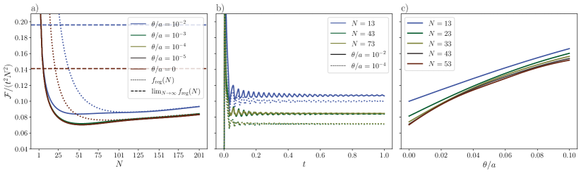
Figure 2: Representation of the different relations of $\mathcal{F}/(t^{2}N^{2})$ with respect to important parameters of the problem. We use a value of $a=100$. We only plot $N$-odd values of the number of particles (the value is 0 otherwise). a) Relation between the $\mathcal{F}/(t^{2}N^{2})$ and the number of particles used (recall that $N$ is always odd) for different ratios of $\theta/a$. The simulation is performed in a time $t=1000$. It is clear in the figure that we reach maximum scaling $\mathcal{F}\sim t^{2}N^{2}$. Two regression functions (shown in dotted lines) of the form $f_{\rm reg}(N)=k_{1}+k_{2}/\sqrt{N}+k_{3}/N$ are shown with their asymptotic convergence (in dashed lines). This are for $\theta/a=0$ in brown, and $\theta/a=10^{-2}$ in blue. The regressions are $f_{\theta/a=0}(N)=0.141-1.193/\sqrt{N}+5.498/N,\ f_{\theta/a=10^{-2}}(N)=0.196-2.311/\sqrt{N}+12.159/N$. We also plot the limits of the regression functions in dashed lines. Both of them converge to the maximum scaling in the limit of a large number of particles. b) Relation of $\mathcal{F}/(t^{2}N^{2})$ with $t$ for different values of $\theta/a$ and $N$. It can be seen that both parameters do not affect how rapidly we reach the approximate time-independent QFI. c) Relation between $\mathcal{F}/(t^{2}N^{2})$ and $\theta/a$ for the different number of particles $N$. The simulation is performed in a time $t=1000$.

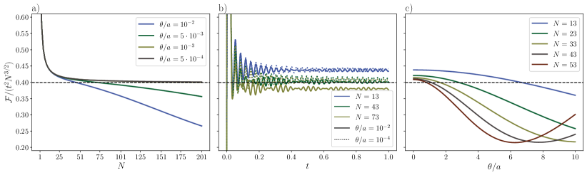
Figure 3: Representation of the different relations of the normalized QFI ($\mathcal{F}/(t^{2}N^{3/2})$) with parameters of the problem. The dashed line represents the QFI from Eq. (50). Furthermore, we use a value of $a=100$. a) Relation between the $\mathcal{F}/(t^{2}N^{3/2})$ and the number of particles used (recall that $N$ is always odd) for different ratios $\theta/a$. The simulation is performed in a time $t=1000$. We see that for a smaller number of particles, we do not require $\theta/a$ to be small. This changes when the number of particles increases. b) Relation of $\mathcal{F}/(t^{2}N^{3/2})$ with $t$ (in natural units) for two different values of ${\theta}/{a}$ and $N$. Changing $\theta/a$ does not affect how fast we reach the time-independent QFI. However, there is a small effect due to $N$. c) Relation between $\mathcal{F}/(t^{2}N^{3/2})$ and $\theta/a$ for different number of particles. The simulation is performed in a time $t=1000$.

Finally, we show that the optimal measurement (i.e. when the CFI and the QFI are equal), is just $S_{x}$. Intuitively, this is the observable that maximizes the CFI as it is the one that potentially will measure the most change from $S_{z}$ without being affected by the one-axis twisting caused by $S_{x}^{2}$. A proof can be found in Appendix D.2.

IV Steady-state metrology

So far we considered the evolution of the probe to be coherent and focused on the $t^{2}$-scaling of the QFI in such a dynamical scenario. Nevertheless, in the limit of large $t$, both environmental noise and timekeeping imprecision are expected to eventually break the unitarity of evolution. In such case, the framework of steady-state metrology offers an alternative way for parameter estimation, that is by readout of the parameter value encoded in the asymptotic steady-state of the dynamics. To this purpose, we consider the following two canonical and physically-motivated classes of steady states, i.e. those induced by A) dephasing and B) thermalization.

IV.1 Dephasing metrology: the case of the diagonal ensemble

As treated in Section III, the long-term evolution governed by the Hamiltonian $H_{\theta}$ in Eq. (1) leads to a Fisher information that is governed by the pinching (dephasing) of the signal $H_{S}$ in the eigenbasis of $H_{\theta}$. That is, the dynamical QFI then corresponds to the variance of the pinched signal Hamiltonian on the initial state, Eq. (23). However, to resolve such dynamical susceptibility in the final state one needs to have an increasingly precise timekeeping device. In contrast, if the timekeeping precision is finite, in the large $t$ limit the system will be effectively described by the steady state of the dephasing map (pinching) applied on the initial state itself as shown in Eq. (19). In sharp contrast to the dynamical case this state has no time dependence. Nevertheless, since the eigenbasis of $H_{\theta}$ depends on the parameter so does the steady-state $\rho_{\theta}$.

We will now assume that the Hamiltonian $H_{\theta}$ has a non-degenerate spectrum around $\theta$, with a minimal energy gap $E$. When the energy gap is closing the dephasing map in Eq. (19) becomes discontinuous and the QFI of $\rho_{\theta}$ diverges. For a non-degenerate $H_{\theta}$ the dephasing map is thus of the form

$$\rho_{\theta}=\mathcal{D}_{H_{\theta}}(\psi)=\sum_{k}\outerproduct{\varphi_{k}^{\theta}}{\varphi_{k}^{\theta}}\psi\outerproduct{\varphi_{k}^{\theta}}{\varphi_{k}^{\theta}},$$ (51)

where $\{\ket{\varphi_{k}^{\theta}}\}$ is the eigenbasis of $H_{\theta}$. Here, first-order perturbation theory yields

$$\ket{\dot{\varphi}_{k}}=\sum_{j\neq k}\ket{\varphi_{j}}\frac{\bra{\varphi_{j}}H_{S}\ket{\varphi_{k}}}{E_{k}-E_{j}},$$ (52)

where we dropped the $\theta$ index and introduced $E_{k}=\bra{\varphi_{k}}H_{\theta}\ket{\varphi_{k}}$. This can be conveniently rewritten as

$$\ket{\dot{\varphi}_{k}}=-\mathrm{i}S\ket{\varphi_{k}}\quad\text{with}\quad S:=\mathrm{i}\sum_{j\neq k}\frac{\outerproduct{\varphi_{j}}{\varphi_{j}}H_{S}\outerproduct{\varphi_{k}}{\varphi_{k}}}{E_{k}-E_{j}}$$ (53)

where $S$ is Hermitian $S^{\dagger}=S$ and “off-diagonal” $\bra{\varphi_{k}}S\ket{\varphi_{k}}=0$. That is, $S$ is the generator of the local rotation of the eigenvectors $\ket{\varphi_{k}}$ of $H_{\theta}$.

To bound the QFI of the dephasing channel in Eq. (51) we proceed in two steps. First, we derive a general bound in terms of the operator $S$, valid whenever $\ket{\dot{\varphi}_{k}}=-\mathrm{i}S\ket{\varphi_{k}}$. Second, we compute the bound in terms of $H_{S}$ for the specific form of $S$ in Eq. (53).

QFI of general dephasing maps

– Observe that the output of the dephasing channel $\rho_{\theta}=\mathcal{D}_{H_{\theta}}(\psi)$ in Eq. (51) with $\ket{\dot{\varphi}_{k}}=-\mathrm{i}S\ket{\varphi_{k}}$ reads

$$\dot{\rho}_{\theta} =-\mathrm{i}[S,\mathcal{D}_{H_{\theta}}(\psi)]+\mathrm{i}\,\mathcal{D}_{H_{\theta}}([S,\psi])=\dot{\rho}_{\rm ext}+\dot{\rho}_{\rm int}\,.$$ (54)

Clearly, $\rho_{\theta}$ and $\dot{\rho}_{\rm int}=\mathrm{i}\mathcal{D}_{H_{\theta}}([S,\psi])$ are diagonal in the dephasing basis, while $\dot{\rho}_{\rm ext}=-\mathrm{i}[S,\mathcal{D}_{H_{\theta}}(\psi)]$ is off-diagonal. This decomposition can be used to simplify the QFI as

$$\mathcal{F} =\Tr[(\dot{\rho}_{\rm ext}+\dot{\rho}_{\rm int})\mathbb{J}^{-1}_{\rho_{\theta}}[\dot{\rho}_{\rm ext}+\dot{\rho}_{\rm int}]]\,.$$ (55)

In fact, $\mathbb{J}^{-1}_{\rho_{\theta}}$ is linear, and satisfies by definition $\dot{\rho}_{\rm int(ext)}=\frac{1}{2}\{\mathbb{J}^{-1}_{\rho_{\theta}}[\dot{\rho}_{\rm int(ext)}],\rho_{\theta}\}$. From this identity it is clear that $\mathbb{J}^{-1}_{\rho_{\theta}}[\dot{\rho}_{\rm int(ext)}]$ is diagonal (off-diagonal) just like $\dot{\rho}_{\rm int(ext)}$ is. Hence, the cross terms in Eq. (55) vanish, and the QFI decomposes as the sum of two contributions

$$\mathcal{F}=\underbrace{\Tr[\dot{\rho}_{\rm ext}\mathbb{J}^{-1}_{\rho_{\theta}}[\dot{\rho}_{\rm ext}]]}_{=\mathcal{F}_{\rm ext}}+\underbrace{\Tr[\dot{\rho}_{\rm int}\mathbb{J}^{-1}_{\rho_{\theta}}[\dot{\rho}_{\rm int}]]}_{=\mathcal{F}_{\rm int}}\;.$$ (56)

The two terms admit a simple intuitive interpretation, as summarized by the following result.

Result 4.

The quantum Fisher information of the dephasing channel $\rho_{\theta}=\mathcal{D}_{H_{\theta}}(\psi)=\sum_{k}\outerproduct{\varphi_{k}}{\varphi_{k}}\psi\outerproduct{\varphi_{k}}{\varphi_{k}}$ with $\ket{\dot{\varphi}_{k}}=-\mathrm{i}S\ket{\varphi_{k}}$ is given by

$$\mathcal{F}=\mathcal{F}_{\rm ext}+\mathcal{F}_{\rm int}\,.$$ (57)

Here, $\mathcal{F}_{\text{\rm ext}}$ is the QFI due to the rotation $\dot{\rho}_{\rm ext}=-\mathrm{i}[S,\rho_{\theta}]$, generated by the Hermitian operator $S$ on the dephased state $\rho_{\theta}=\mathcal{D}_{H_{\theta}}(\psi)$, and $\mathcal{F}_{\rm int}$ is the Fisher information of the distribution $p_{k}=\bra{\varphi_{k}}\psi\ket{\varphi_{k}}$.

Upper bounds for dephasing metrology with Hamiltonian control

– Let us now take $S$ to be of the particular form given in the Eq. (53) with a bounded energy gap $|E_{k}-E_{j}|\geq E\,\,\forall\,\,k,j$. We want to express the right-hand side of Eq. (57) in terms of the Hamiltonian $H_{S}$ and the gap $E$. The expression we obtain is given by the following result.

Result 5.

For any input state $\psi$ let $\rho_{\theta}=\mathcal{D}_{H_{\theta}}(\psi)$ be the state resulting from the application of the dephasing Eq. (51) with a nondegenerate Hamiltonian $H_{\theta}=H_{C}+\theta H_{S}$ with all energies gapped by at least $E$. The QFI of the state $\rho_{\theta}$ is upper-bounded by

$$\mathcal{F}\leq\frac{(3+\pi^{2})}{3}\frac{\|H_{S}\|^{2}}{E^{2}}\;,$$ (58)

where $\|H_{S}\|=\lambda_{\rm max}^{S}-\lambda_{\rm min}^{S}$, as in Sec. III.

The proof of this result can be found in Appendix E and relies on maximizing separately $\mathcal{F}_{\rm ext}$ and $\mathcal{F}_{\rm int}$. Thanks to the interpretation of both $\mathcal{F}_{\rm ext}$ and $\mathcal{F}_{\rm int}$ corresponding to QFI induced by (external and internal) rotations induced by the generator $S$, the proof relies on bounding the operator norm of $S$, for which we employ Gershgorin’s theorem (see Appendix A.5 and Ref. [68]).

IV.1.1 Saturable scaling for dephasing metrology with Hamiltonian control

The bound in Eq. (58) cannot be saturated in general. However, if the Hamiltonian control is unrestricted it is generally possible to reach the same scaling $\mathcal{F}\sim\|H_{S}\|^{2}/E^{2}$ up to a constant prefactor. In particular, let us assume that one can prepare an initial product state $\ket{\psi}$ which is an eigenstate of $H_{S}$ exactly the middle of the spectrum. This is motivated by local $H_{S}$, where (for even N) $\ket{\psi}$ can be prepared by initializing half of the particles ”up” and half ”down”. In the Appendix E.2 we then show the following result.

Result 6.

For any signal Hamiltonian $H_{S}$ with extremal eigenvalues $\lambda_{\rm min}^{S}$ and $\lambda_{\rm max}^{S}$ and the initial state $\ket{\psi}$ satisfying $H_{S}\ket{\psi}=\frac{\lambda_{\rm min}^{S}+\lambda_{\rm max}^{S}}{2}\ket{\psi}$, there exist a control Hamiltonian $H_{C}$ such that the QFI of the dephased state $\rho_{\theta}=\mathcal{D}_{H_{\theta}}(\psi)$ in Eq. (51) equals

$$\mathcal{F}=\frac{3}{2}\frac{\|H_{S}\|^{2}}{E^{2}}\,,$$ (59)

where $E$ is the minimal energy gap of the (nondegenerate) Hamiltonian $H_{\theta}=H_{C}+\theta H_{S}$, and $\|H_{S}\|=\lambda_{\rm max}^{S}-\lambda_{\rm min}^{S}$.

We now sketch a proof of the result. Without loss of generality, we can consider the situation around $\theta=0$. Let us denote by $\ket{\Phi_{\downarrow}}$ and $\ket{\Phi_{\uparrow}}$ the extremal eigenstates of $H_{S}$ corresponding to the eigenvalue $\lambda_{\text{min}}^{S}$ and $\lambda_{\text{max}}^{S}$ respectively. Since we have full freedom to choose the control Hamiltonian $H_{C}$ we will take it block-diagonal with respect to the qutrit subspace $\text{span}\{\ket{\Phi_{\uparrow}},\ket{\psi},\ket{\Phi_{\downarrow}}\}$. For such choice, the dephasing dynamics for any $\theta$ leaves the initial state $\ket{\psi}$ inside this subspace. Thus, in this setting, the freedom to choose the control Hamiltonian with a bounded energy gap boils down to let $H_{C}$ run through all $3\times 3$ Hermitian matrices with non-degenerate eigenvalues separated by at least $E$. With the help of the Result 4, in appendix 4 we optimise $\mathcal{F}_{\text{int}}$ for all real $H_{C}$ and find that the choice

$$H_{C}=\frac{E}{\sqrt{2}}\left(\begin{array}[]{ccc}0&1&0\\ 1&0&1\\ 0&1&0\\ \end{array}\right)$$ (60)

in the basis $\{\ket{\Phi_{\uparrow}},\ket{\psi},\ket{\Phi_{\downarrow}}\}$ has the energy spectrum $(E,0,-E)$, and for the dephased state $\rho_{\theta}=\mathcal{D}_{H_{\theta}}(\psi)$ gives $\mathcal{F}=\mathcal{F}_{\text{int}}+\mathcal{F}_{\text{ext}}$ in Eq. (59).

IV.1.2 Interacting spins probe

Similar to Sec. III, we now apply our general considerations to the estimation of the magnetic field strength ($H_{S}=\frac{1}{2}\sum_{i=1}^{N}\sigma_{z}^{(i)}$) via a interacting spins probe with two-body control as given in Eq. (4). We consider as initial product state

$$\ket{\psi}=\ket{-y}^{\otimes N},$$ (61)

where $\ket{-y}$ is an eigenstate of $\sigma_{y}$. To compute the asymptotic QFI, $\mathcal{F}$, in the long-time limit, we project the initial state $\ket{\psi}$ onto the eigenbasis of $H_{\theta}$, and remove coherence between different eigenspaces. Notice that, in this process, we do not remove coherence between eigenstates belonging to the same eigenspace, and we do not remove coherence between eigenstates whose energy difference is proportional to the infinitesimal increment of $\theta$ necessary to compute the QFI.

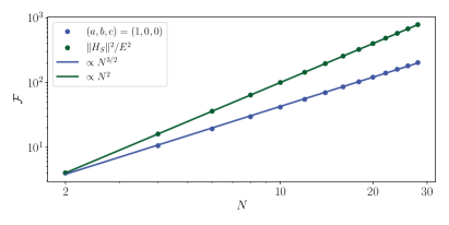
Figure 4: QFI, as a function of $N$, for $\theta=0$. The blue dots correspond to $\mathcal{F}$ computed for $(a,b,c)=(1,0,0)$, while the green dots represent $\|H_{S}\|^{2}/E^{2}$. The continuous lines are references to visualize the $N^{3/2}$ and $N^{2}$ scaling.

Result 7.

Let $H_{\theta}$ be the Hamiltonian of the form $H_{\theta}=\theta H_{S}+H_{C}$, with $H_{S}=\frac{1}{2}\sum_{i=1}^{N}\sigma^{(i)}_{z}$ a local Hamiltonian, and $H_{C}$ the control term with only two-body interactions as given in Eq. (4). Let the initial state be a product state as given in Eq. (61), and consider the corresponding long-time averaged state as given by $\mathcal{D}_{H_{\theta}}(\psi)$. Then, by a proper choice of $H_{C}$, the QFI evaluated at $\theta=0$ of $\mathcal{D}_{H_{\theta=0}}(\psi)$ behaves as

$$\mathcal{F}\approx A\frac{N^{3/2}}{E^{2}}+\order{N}\,,$$ (62)

where $A\approx 1.34$ at least up to $N\leq 30$ (see numerical results in Fig. 4).

Indeed, in Fig. 4 we plot $\mathcal{F}$, as a function of $N$, as blue dots in the $(a,b,c)=(1,0,0)$ case, and we compute the QFI around $\theta=0$. We consider even values of $N$ since odd values yield a lower QFI. Interestingly, from the numerics we find an $N^{3/2}$ scaling, confirming a super-linear scaling of the QFI, enabled by interactions, also in this scenario with decoherence.

As a comparison, in Fig. 4 we further plot as green dots the ratio $\|H_{S}\|^{2}/E^{2}$ which appears in the upper bound in Eq. (58). While this upper bound is saturated for $N=2$, we see that it scales as $N^{2}$, thus it is not saturated with this choice of the interaction for larger values of $N$.

Finally, we computed the ratio between the QFI for arbitrary choices of $(a,b,c)$, and the upper bound $\|H_{S}\|^{2}/E^{2}$, and we found numerical evidence that $(a,b,c)=(1,0,0)$ maximizes this ratio (note, however, that other choices of $(a,b,c)$ could yield a higher QFI). It remains an interesting open question to explore alternative interacting spins geometries that can approach the $N^{2}$ scaling for the long time-averaged state.

IV.2 Gibbs ensemble metrology

While dephasing might be interpreted as an effective noise induced by the finiteness of time resolution, non-unitary dynamics can, more generally, affect metrological probes that are not perfectly isolated from environmental degrees of freedom. A rather general example of noisy evolutions are those leading to thermal equilibrium, i.e. where the steady state of the probe is given by the Gibbs state

$$\rho_{\theta}=\frac{e^{-\beta H_{\theta}}}{\Tr[e^{-\beta H_{\theta}}]}\,,$$ (63)

for some temperature $T=(k_{\rm B}\beta)^{-1}$.

The expression for the Fisher information in such case takes the form of a generalized variance (see e.g. [69, 4, 70])

$$\mathcal{F}=\beta^{2}\left(\Tr[H_{S}\mathcal{J}_{\rho_{\theta}}[H_{S}]]-\Tr[\rho_{\theta}H_{S}]^{2}\right)\;,$$ (64)

where $\mathcal{J}_{\rho}$ is a superoperator that acts, in the basis of eigenvectors of $\rho\equiv\sum_{i}p_{i}\outerproduct{i}{i}$, as

$$\mathcal{J}_{\rho}[\outerproduct{i}{j}]=2\frac{(p_{i}-p_{j})^{2}}{(\ln p_{i}-\ln p_{j})^{2}(p_{i}+p_{j})}\outerproduct{i}{j}\;.$$ (65)

In the semi-classical case in which $[\rho_{\theta},H_{S}]=0$ (equivalently $[H_{C},H_{S}]=0$) the expression in Eq. (64) reduces to the standard variance of $H_{S}$ computed on $\rho_{\theta}$, while it is smaller otherwise [4].

While previous works have considered metrological probes at thermal equilibrium, the fundamental limits of this approach and the corresponding optimal control (that is, $\max_{H_{C}}\mathcal{F}_{\theta}$ for given $H_{S}$) have been recently obtained in [4]. For completeness, we now briefly mention the main results obtained there.

Result 8 (Optimal metrology at thermal equilibrium [4]).

When assuming no restriction on the possible form of the control values $H_{C}$ and finite temperature $0<\beta<\infty$, the maximum (saturable) value of the Fisher information at thermal equilibrium in Eq. (64) is given by

$$\mathcal{F}\leq\beta^{2}\frac{\|H_{S}\|^{2}}{4}\;.$$ (66)

where $\|H_{S}\|=\lambda_{\max}^{S}-\lambda_{\min}^{S}$.

Notice that this bound, as the other ones depending on $\|H_{S}\|^{2}$, entails a Heisenberg-like scaling $\propto N^{2}$ of the Fisher information in terms of the number of particles, and diverges in the limit of zero temperature $\beta\rightarrow\infty$. This is because the state in Eq. (21) becomes the ground state in such limit, which can in principle have infinitely sharp transitions between microstates whenever there are crossovers of energy between the ground and the first-excited states. Indeed, a meaningful bound can still be obtained in this limit, under the additional restriction of the system being gapped, obtaining [4]

$$\mathcal{F}_{\rm{low-T}}\leq\frac{\|H_{S}\|^{2}}{\Delta_{g}^{2}}+\mathcal{O}(e^{-\beta\Delta_{g}})\;,$$ (67)

where $\Delta_{g}$ is the spectral gap.

IV.2.1 Interacting spins probe

As in the previous Sections, we now focus on the estimation of the strength of a magnetic field ($H_{S}=\frac{1}{2}\sum_{i=1}^{N}\sigma_{z}^{(i)}$) via a interacting spins probe with two-body control as given in Eq. (4), which is now prepared in a Gibbs states as in Eq. (63). Our main result is to show that the upper bound in Eq. (66) can be easily saturated in this case.

Result 9.

Let $H_{\theta}$ be the Hamiltonian of the form $H_{\theta}=\theta H_{S}+H_{C}$, with $H_{S}=\frac{1}{2}\sum_{i=1}^{N}\sigma^{(i)}_{j}$ a local Hamiltonian, and $H_{C}$ the control term with only two-body interactions as given in (4). Then, by taking $c\gg 1$ and $a=b=0$, the thermal QFI evaluated at $\theta=0$ reads

$$\mathcal{F}\approx\frac{\beta^{2}N^{2}}{4}\,,$$ (68)

thus saturating the upper bound (66).

To show this result, first note that $H_{S}$ and $H_{C}$ commute. In this case the QFI in (64) simplifies to the variance of $H_{S}$:

$$\mathcal{F}=\beta^{2}\left(\Tr[H_{S}^{2}\rho_{\theta}]-\Tr[\rho_{\theta}H_{S}]^{2}\right)\;,$$ (69)

This variance is maximised for the state $\rho_{\theta}=\frac{1}{2}\left(\outerproduct{\lambda_{\max}^{S}}{\lambda_{\max}^{S}}+\outerproduct{\lambda_{\min}^{S}}{\lambda_{\min}^{S}}\right)$ where $\ket{\lambda_{\min}^{S}}=\ket{1,...,1}$ and $\ket{\lambda_{\max}^{S}}=\ket{0,...,0}$. Now, we wish to encode this state in a Gibbs state as in (63). For $\theta=0$, the corresponding Gibbs state is simply

$$\rho_{0}=\frac{e^{-\beta H_{C}}}{\Tr[e^{-\beta H_{C}}]}\,.$$ (70)

By taking $c\gg 1$ (with $a=b=0$), the corresponding Gibbs state becomes the desired state $\rho_{\theta}\approx\frac{1}{2}\left(\outerproduct{1,...,1}{1,...,1}+\outerproduct{0,...,0}{0,...,0}\right)$ up to exponentially small corrections of order $\mathcal{O}(\exp(-\beta c))$. A direct application of (69) then gives the desired result (68).

V Transient regime: From dynamical to steady state

The main goal of this last section is to characterize the behavior of the QFI in the transient regime, before reaching the steady states described in the previous Sections (diagonal and Gibbs ensemble). Furthermore, we also analyze other types of physically relevant noise, e.g. local and global decoherence.

The dynamics of the probe are assumed Markovian and described by the Lindblad master equation introduced in Eq. (22). Following the previous sections, we take a probe consisting of $N$ spin-$\frac{1}{2}$ systems with a symmetric Hamiltonian where the signal $H_{S}$ is fixed, $H_{C}$ can be controlled and the dissipators $L_{\theta,i}$ can depend on $H_{\theta}=\theta H_{S}+H_{C}$. The total Hamiltonian reads

$$H_{\theta}(a,b,c)=\theta S_{z}+aS_{x}^{2}+bS_{y}^{2}+cS_{z}^{2}\,,$$ (71)

where the signal term is $S_{z}$ and the control term is of the form of Eq. (4) ($H_{C}=aS_{x}^{2}+bS_{y}^{2}+cS_{z}^{2}$) and features collective two-body interactions with tunable parameters $(a,b,c)$. For the noise model, specified by the dissipators $\sqrt{\gamma_{i}}L_{\theta,i}$, we consider four physically motivated scenarios in the sections below: dephasing, thermalization, global noise, and local noise.

V.1 Dephasing

In this subsection, we study the QFI in the presence of decoherence between the eigenstates. We consider the Hamiltonian in Eq. (71) and the initial state

$$\ket{\psi}=\ket{-y}^{\otimes N},$$ (72)

where $\ket{-y}$ is an eigenstate of $\sigma_{y}\ket{-y}=-\ket{-y}$.

We now consider a finite-time model to analyze the time necessary to reach the asymptotic values leading to Result 7. The model is based on our ignorance about the exact time $t$ for which the evolution takes place. In particular, we assume that the initial state $\ket{\psi}$ in Eq. (72) evolves according to $H_{\theta}$ in Eq. (71) for an unknown time $t$ that satisfies a probability distribution $P(t)$. For simplicity, we assume a flat distribution $P(t)=1/T$, so that the quantum state is described by the time-averaged state, i.e.

$$\rho_{\theta}(T)=\frac{1}{T}\int_{0}^{T}e^{-\mathrm{i}tH_{\theta}}\outerproduct{\psi}{\psi}e^{\mathrm{i}tH_{\theta}}dt\,.$$ (73)

In the limit $T\rightarrow\infty$, we obtain a fully dephased state.

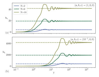
Figure 5: QFI, as a function of time, for $3$ values of $N$ shown in the legend and $\theta=0$. The full lines correspond to the finite-time QFI of $\rho_{\theta}(T)$ in Eq. (73). The dashed lines represent the asymptotic values of the $\mathcal{F}$. a) is computed choosing $(a,b,c)=(1,0,0)$, and b) with $(a,b,c)=(10^{-1},0,0)$.

In Fig. 5 we plot as full lines the QFI, as a function of time, for three values of $N$ shown in the legend. The dashed lines correspond to the asymptotic values of $\mathcal{F}$. Fig. 5a) corresponds to $(a,b,c)=(1,0,0)$, as in Fig. 4, and Fig. 5b) corresponds to $(a,b,c)=(10^{-1},0,0)$. As expected, the finite-time QFI tends to the asymptotic value after a transient time characterized by an oscillating behavior of $\mathcal{F}$. This time appears to be independent of $N$.

Interestingly, we notice the following fact. If we reduce the interaction by a factor $\lambda$, i.e. we consider $(a,b,c)\to(a,b,c)/\lambda$, the gap between the spectrum scales as $1/\lambda$, leading to the asymptotic value of the $\mathcal{F}$ scaling as $\lambda^{2}$. This is consistent with the first-order perturbation theory result in Eq. (52), and confirmed by the comparison between Fig. 5a) and Fig. 5b), where $\lambda=10$, and the asymptotic value of $\mathcal{F}$ increases by $10^{2}$. This higher value of the QFI is reached after a longer transient time. However, this time only scales with $\lambda$ (as confirmed by Fig. 5). Therefore, by rescaling the interaction by $\lambda$, the asymptotic value of the QFI scales as $\mathcal{F}\propto\lambda^{2}$, whereas the transient time only increases as $\lambda$. In other words, the QFI rate, $\mathcal{F}/t$, increases linearly with $\lambda$. As we will see, this is in stark contrast with the thermal case, studied in Sec. V.2, where an enhancement of the QFI comes at the expense of an exponential increase in the equilibration time.

V.2 Thermalization

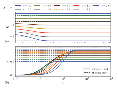
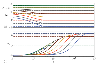
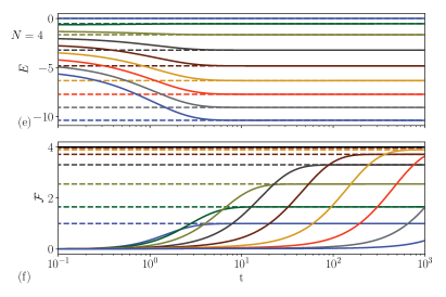
Figure 6: Energy and fisher information as a function of time. Parameters: $N\in\{2,3,4\}$, $\beta=1$, $\gamma=1$, $\theta=0$, initial state $p_{n}=1/(N+1)$.

Here we study how the Fisher information changes, as a function of time, during thermalization. We consider the same Hamiltonian of the previous section but setting $a=b=0$ and $c\neq 0$ so that time evolution can be effectively described by classical stochastic dynamics. Indeed, recall that by taking $c\gg 1$ we can achieve the maximal possible thermal QFI as discussed in Result 9. We assume that each qubit is locally coupled to a thermal bath, which drives the global state towards a thermal state (detailed balance). Denoting with $p_{n}$ the probability of having $n$ excitations in the system, we consider the following rate equation

$$\dot{p}_{n}=-p_{n}\left[\Gamma_{n\to n+1}+\Gamma_{n\to n-1}\right]\\ +p_{n-1}\Gamma_{n-1\to n}+p_{n+1}\Gamma_{n+1\to n}\,,$$ (74)

where $\Gamma_{n\to m}$ represents the transition rate from $n$ to $m$ excitations in the sytem. They are given by

$$\Gamma_{n\to n+1} =\gamma(N-n)f\left[U(n+1)-U(n)\right],$$ (75)

$$\Gamma_{n\to n-1} =\gamma nf\left[U(n-1)-U(n)\right]\,,$$

where $\gamma$ is the thermalization rate, $U(n)$ is the energy of a state with $n$ excitations, and

$$f(x)=\left[1+e^{\beta x}\right]^{-1}\,,$$ (76)

where $\beta$ is the inverse temperature of the system.

In Fig. 6 we plot the energy and the Fisher information, as a function of time. Every two panels correspond to a different value of $N=2,3,4$, and each curve to a different value of $c$ (see the legend). The colored dashed lines represent the thermal distribution, and the black line represents the ultimate limit to the Fisher information, which in this case is given by $\beta^{2}N^{2}/4$ (Result 8).

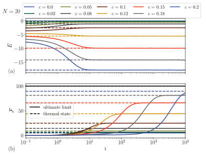
Figure 7: Energy and fisher information as a function of time. Parameters: $N=20$, $\beta=1$, $\gamma=1$, $\theta=0$, initial state $p_{n}=1/(N+1)$.

In Fig. 7 we do the same plot, but we choose a large value of $N=20$, and correspondingly we extend the time-simulation by a factor 10 (we plot until $10^{4}$ and not $10^{3}$). Notice also that we choose smaller values of $c$.

From Figs. 6 and 7, we first observe that the QFI grows with $c$ reaching the value $\mathcal{F}\approx N^{2}/4$ in the limit $c\gg\theta$, which saturates the bound Eq. (66) (note that $\beta=1$ in Fig. 6), as expected from Result 9. Second, we observe a clear tradeoff between the enhancement in the QFI and the thermalization time, as the thermalization time of the QFI grows (exponentially) with $c$ and $N$. It is interesting to note that this slow thermalization does not affect the energy $E$; this can be understood by noting that the QFI highly depends on small perturbations in the population of the thermal state $\rho_{\theta}$ induced by $\theta$. Such changes require crossing a free energy barrier $\Delta F$ that grows linearly with $N$ and $c$ (the time for crossing the barrier via thermal fluctuations grows exponentially with $\Delta F$). Therefore, interaction-based enhancements in the QFI come with the high price of long thermalization times. A similar behavior may arise in other models given the form of the optimal thermal state, $\rho_{\theta}\approx(\ket{0,...,0}\bra{0,...,0}+\ket{1,...,1}\bra{1,...,1})/2$, with the population concentrated into two locally stable states. Indeed, in the case of thermometry, tradeoffs between enhanced sensitivity and long thermalization times have been characterised [71].

V.3 Global noise

The previous case studies showed that interactions can enhance $\mathcal{F}$ in the presence of dephasing and thermalizing noise. Here we extend these considerations to another relevant case of (global) noise.

We consider a global noise $S_{x}$ with a parameter strength $\gamma$, and $H_{\theta}=H_{C}+\theta S_{z}$. That is, in Eq. (22), $L_{\theta,i}=S_{x}$ and $\gamma_{i}=\gamma$.

We use $H_{C}=aS_{x}^{2}$ as the control Hamiltonian. If we choose $a$ to be some large constant compared to $\theta$. This gives us

$$H_{\theta}=\theta S_{z}+aS_{x}^{2}\,.$$ (77)

Then under the same conditions used to obtain Eq. (50) and measuring $S_{x}$ (as in Sec. III.2.2), we find that the CFI ($\mathcal{I}$) is

$$\mathcal{I}_{\rm control}=4\dfrac{(1-\mathrm{e}^{-t{\gamma/2}})^{2}}{{\gamma^{2}}}\frac{N^{3/2}}{\sqrt{2\pi}}+\order{\frac{1}{a}}\,.$$ (78)

This can be contrasted to the QFI obtained in the absence of control:

$$\mathcal{F}_{\text{no control}}=4\dfrac{(1-\mathrm{e}^{-t{\gamma/2}})^{2}}{{\gamma^{2}}}N\,.$$ (79)

Hence, we obtain a $N^{1/2}$ fold enhancement by appropriately tuning the interactions, which in this case does not come at the price of longer equilibration times.

V.4 Local Noise

In the previous sections, we analyzed models of noise that involve global dissipators (in the thermalization case, even if the starting point is a local microscopic model with a thermal bath locally coupled to each qubit, the dissipators become global after performing the secular approximation). Many relevant noise models however involve local noise operators. To analyze this scenario, we consider the same model as in Sec. V.3 but replace the global noise operators $S_{x}$ with a collection of local noise operators $\sigma_{x}^{(i)}$ acting on every site $i$. The Hamiltonian is the same as Eq. (77), and the initial state is

$$\ket{\psi}=\ket{y}^{\otimes N}\,,$$ (80)

whith $\ket{y}$ the eigenstate of $\sigma_{y}\ket{y}=\ket{y}$. For details on the simulation see Appendix A.6.

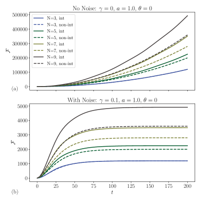
Figure 8: QFI, as a function of time, in the noiseless case (upper panel) and in the presence of local noise (lower panel). Each color corresponds to a different value of $N$ (see legend). The dashed line corresponds to the non-interacting case and the full line to the interacting case. Parameters are indicated in the panel title.

In Fig. 8 we plot the QFI, as a function of time, in the noiseless case (upper panel) and in the presence of local noise (lower panel). Each color corresponds to a different value of $N$, while the dashed line corresponds to the non-interacting case (i.e. $H_{C}=0$), and the full line to the interacting case.

As we expected, in the noiseless case (upper panel) the interacting case outperforms the non-interacting case, and the advantage visibly scales with $N$ (there is hardly any advantage for $N=3$, while it is quite pronounced for $N=9$).

In the presence of noise (lower panel) the QFI does not increase indefinitely with time, but it saturates to a final value. Interestingly, such final value is enhanced by the interaction, and the advantage increases also in this case with $N$.

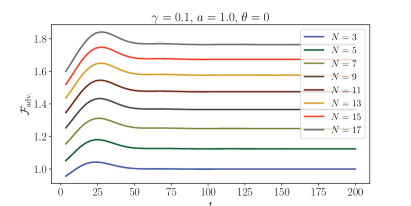
Figure 9: Ratio between the QFI in the interacting and non-interacting case, as a function of $t$, in the presence of local noise. Parameters in the panel title.

In Fig. 9 we plot $\mathcal{F}_{\text{adv.}}$, defined as the ratio between the QFI in the interacting and non-interacting case. As we can see, the advantage enabled by the interaction scales with $N$, and here we display values up to $N=17$.

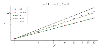
Figure 10: Log-log plot of the asymptotic (long-time) value of the QFI, in the presence of noise, as a function of $N$. The dashed lines are references to distinguish the $N$ scaling.

As clearly visible in Figs. 8 and 9, the QFI saturates to a finite value for large times. In Fig. 10 we plot such “asymptotic” value of the QFI as a function of $N$. As we can see, the asymptotic QFI scales superlinearly in $N$.

VI Conclusion

In this work, we considered the precision limits of many-body quantum probes. Given a signal Hamiltonian that encodes an unknown parameter $\theta$ into the probe’s state, see Eq. (1), we considered the maximization the QFI over all control Hamiltonians. We considered two main scenarios: (i) Dynamical, i.e., unitary evolution driven by $H_{\theta}$ given an initial eigenstate of $H_{S}$, and (ii) Steady-state, with focus on the Gibbs $\propto\exp(-\beta H_{\theta})$ and diagonal $\mathcal{D}_{H_{\theta}}[\rho]$ ensembles. For each case, we presented upper bounds on the QFI as well as corresponding interacting control Hamiltonians that can approach such bounds. Our main results are summarized in Table 1.

Having established general results for arbitrary encoding $H_{S}$, we focused on the estimation of the strength of a magnetic field via a $N$-interacting spins with two-body interactions. We showed that a carefully engineered central-spin model (Eq. (39)), as well as an spin-squeezing model (Eq. (4)), can saturate the dynamical upper bound $\mathcal{F}\sim t^{2}N^{2}$ when starting with an initial product state for the probe. Likewise, we also showed that the thermal bound $\mathcal{F}\sim\beta^{2}N^{2}$ can be saturated with the collective spin model as in Eq.  (4), whereas it enables a QFI scaling as $\mathcal{F}\sim N^{3/2}/E^{2}$ for the diagonal ensemble. Our results for the $N$-spin probe are summarized in Table 2.

Finally, we explored connections between the two scenarios, studying the transient regime connecting the dynamical and steady-state scenarios for the $N$-spin probe. We observed tradeoffs between an enhanced sensitivity of the steady state and the time required to reach it for both Gibbs and diagonal ensembles. We also considered other models of Markovian noise, namely local and global decoherence, showcasing advantages in the sensitivity arising due to the presence of interactions in the network.

These results provide new insights into the potential and limits of many-body metrology [5], and set the stage for the realization of highly sensitive interacting spin sensors. For steady-state metrology, an important open question for the future is to generalize the QFI bounds to general non-equilibrium steady states of open quantum systems (see e.g. [37, 38, 39, 40, 41, 42]) given arbitrary control on $H_{C}$. Characterizing optimal many-body Hamiltonian control for multiparameter parameter estimation [56, 72, 73, 74, 75] is another exciting future challenge. Other interesting future directions include exploring connections with other frameworks for many-body parameter estimation [56, 72] as well as QFI optimization in many-body systems [76, 77, 78, 79, 80], and Hamiltonian learning [81, 82].

oneΔ

Appendix A Preliminaries

In this section, we provide a concise overview of key analytical tools and concepts that will be referenced throughout the subsequent sections.

A.1 Derivative of the exponential operator

Here we briefly summarize how to take the derivative of the exponential of a Hamiltonian that depends on a parameter $x$. We refer the reader to Ref. [83] for further details.

Assume we have a Hamiltonian $H$ that depends on a parameter ${x}$, i.e. $H=H({x})$. Then we can compute the derivative of the exponential of this operator with respect to $x$ as follows

$$\frac{d}{dx}e^{-\beta H({x})}=-\beta\int_{0}^{1}e^{-s\beta H({x})}\frac{d}{dx_{i}}H({x})e^{-(1-s)\beta H({x})}ds\,,$$ (81)

for some $\beta\in\mathbb{C}$.

A.2 Time-independent perturbation theory

Here we explain the basic concepts necessary to understand how perturbation theory is used in this paper to derive results. For a more in-depth analysis check Ref. [84].

We start by tackling the non-degenerate case. Let us consider a physical system in the form of

$$H=H_{0}+xV\,,$$ (82)

where $x$ is a small parameter. Then $V$ can be treated as a perturbation of the system. In this limit, we can approximate the eigenvectors and eigenvalues of $H$ with the ones of $H_{0}$ and some corrections. Indeed, we can expand the eigenvalues/eigenvectors of $H$ (denoted as $\overline{E_{i}},\ \ket{\overline{E_{i}}}$) as a power series of $x$ and the eigenvalues/eigenvectors of $H_{0}$ (denoted as $E_{i}$, $\ket{E_{i}}$). In the limit of $x\to 0$, we can approximate this power series at just the first order. Under this approximation, the eigenvectors of $H$ are

$$\ket{\overline{E_{i}}}=\ket{E_{i}}+x\sum_{j\neq i}\frac{\bra{E_{i}}V\ket{E_{j}}}{E_{i}-E_{j}}\ket{E_{j}}+\order{x^{2}}\,,$$ (83)

and similarly, the energies are

$$\overline{E_{i}}=E_{i}+x\expectationvalue{V}{E_{n}}+\order{x^{2}}\,.$$ (84)

When $H_{0}$ is degenerate, the previous sum in Eq. (83) can diverge. Indeed, it will only converge if the term $\bra{E_{i}}V\ket{E_{j}}$ is zero when $E_{i}-E_{j}=0$. This means that the perturbative expansion has a preferred basis. And this is the one that fulfills

$$\bra{E_{i,1}}V\ket{E_{i,2}}=0\,,$$ (85)

where we denote $\ket{E_{i,j}}$ as the $i$-th excited state and the index $j$ accounts for the different states with the same energy. Therefore, the preferred basis is the one in which the unperturbed states are orthogonal under the action of $V$, or in other words, the one which ensures that Eq. (83) does not diverge.

A.3 Tensor product of N spin-$\frac{1}{2}$ as the linear combination of Dicke states

We first define a Dicke state. The Dicke states are eigenvectors of $S_{z}$ and $S^{2}$. Recall that

$$S_{z}=\frac{1}{2}\sum_{i}\sigma_{z}^{(i)}\,,$$ (86)

where $\sigma_{z}^{(i)}$ represents the Pauli matrix z acting in the $i$-th particle. Furthermore, $S^{2}$ is the total spin of the state. These states are usually written as $\ket{S,m_{z}}$ where $S$ represents the total spin (proportional to the eigenvalues of $S^{2}$) and $m_{z}\in[-S,S]$ are the eigenvalues of $S_{z}$, the $z$ component of this spin.

With this, we are ready to define spin-coherent states. Take one vector in the Bloch sphere to be $\ket{\vartheta,\phi}=\cos\tfrac{\theta}{2}\ket{0}+e^{-i\phi}\sin\tfrac{\theta}{2}\ket{1}$ where $\vartheta,\phi$ are polar and azimuthal angles respectively. Then if we take the tensor product of $N$ of this state we can rewrite the state as follows [85]

$$\ket{\vartheta,\phi}^{\otimes N}=\frac{1}{(1+|\eta|^{2})^{S}}\sum_{m_{z}=-S}^{S}\binom{2S}{S+m_{z}}^{1/2}\eta^{S+m_{z}}\ket{S,m_{z}}\,.$$ (87)

where $\eta=-\tan\left(\frac{\vartheta}{2}\right)e^{-\mathrm{i}\phi}$. Furthermore, without loss of generality, we can take $\vartheta,\phi$ with respect to the $x$-axis of the Block sphere. By doing so, we can move from expressing the state in the basis of $S_{z}$, $\{\ket{S,m_{z}}\}_{m_{z}=-S}^{S}$ to the basis of $S_{x}$, $\{\ket{S,m_{x}}\}_{m_{x}=-S}^{S}$. Notice that here we write $m_{x}$ to emphasize that we are on the basis of $S_{x}$. Then we can rewrite Eq. 87 in this basis by

$$\ket{\vartheta_{x},\phi_{x}}^{\otimes N}=\frac{1}{(1+|\eta|^{2})^{S}}\sum_{m_{x}=-{S}}^{S}\binom{2{S}}{{S}+m_{x}}^{1/2}\eta^{{S}+m_{x}}\ket{{S},m_{x}}\,,$$ (88)

where we also emphasize that the reference for $\vartheta_{x},\phi_{x}$ is the $x-$axis in the Block sphere.

A.4 Vectorisation formalism

Here we will cover the basics of the vectorization formalism that are useful to understanding this manuscript. For a more in-depth review please refer to Ref. [86]. Vectorization is a linear operator defined as follows

$$\begin{matrix}\mathrm{vec}:&\left(\mathbb{C}^{d}\right)&\to&\left(\mathbb{C}^{d}\right)^{\otimes 2}\\ \quad\\ &A=\sum_{i,j}^{d}A_{i,j}\outerproduct{i}{j}&\to&|{{A\rangle}\!\rangle}=\sum_{i,j}A_{i,j}\ket{i}\ket{j^{*}}\,,\end{matrix}$$ (89)

where $\ket{j^{*}}$ denotes the conjugate of $\ket{j}$.

A basic property of the vectorization formalism that is very useful is the following. Given $A,B,C$ three matrices that can be multiplied as follows $ABC$, then

$$|{{ABC\rangle}\!\rangle}=A\otimes C^{T}|{{B\rangle}\!\rangle}\,,$$ (90)

where we emphasize that $C^{T}$ is the transpose of $C$. Furthermore, we can see that

$$\langle\!\langle A|B\rangle\!\rangle=\langle\!\langle\mathbbm{1}|A^{\dagger}B\otimes\mathbbm{1}|\mathbbm{1}\rangle\!\rangle=\sum_{i,j}\bra{i}\bra{{i}^{*}}A^{\dagger}B\otimes\mathbbm{1}\ket{j}\ket{{j}^{*}}=\Tr[A^{\dagger}B]\,.$$ (91)

Finally, we show the form of a super-operator in the vectorized form. We denote the vectorized form of a super-operator $\Phi(\cdot)=\sum A_{i}(\cdot)B_{j}^{\dagger}$ as

$$\hat{\Phi}:={\rm Vec}\left[\Phi(\cdot)\right]=A_{i}\otimes{B}_{j}^{*}\,,$$ (92)

where $B^{*}$ is the conjugate of $B$.

A.5 Gershgorin’s circle theorem

We present a simplified version of Gershgorin’s circle theorem [68] that we use in Appendix E.1 in order to upper bound the eigenvalues of an hermitian matrix.

Proposition 1.

Consider a $n\times n$ hermitian matrix $M$ and denote $\lambda_{\rm max}^{M}$ as the largest eigenvalue of $M$. Denote the elements of this matrix by $M_{i,j}$. Then given that the sum of elements in any row is upper bounded by some value $E$, that is $\sum_{j}|M_{ij}|\leq E$ for any $i\in\{1,...,n\}$, the largest eigenvalue of $M$ can be bounded by $E$ as

$$\lambda_{\rm max}^{M}\leq E\;\;.$$ (93)

This theorem gives a simple way to upper-bound the eigenvalues of any hermitian matrix.

A.6 Simulations of local noise.

The simulations of Figs. 8, 9, 10 have been done with QuTip and the “Permutational Invariant Quantum Solver (PIQS)”. For numerical reasons we do this analysis in a rotated (but equivalent) frame: it is more convenient to have a dissipator that depends on $\sigma_{z}^{(i)}$ rather than $\sigma_{x}^{(i)}$. We therefore consider a unitary transformation such that

$$\sigma_{z}^{(i)} \to\sigma_{x}^{(i)},$$ (94)

$$\sigma_{x}^{(i)} \to\sigma_{z}^{(i)},$$ (95)

$$\sigma_{y}^{(i)} \to-\sigma_{y}^{(i)}.$$ (96)

With this transformation, the Hamiltonian $H_{\theta}^{\rm original}=\theta S_{z}+aS_{x}^{2}$ becomes

$$H_{\theta}=\theta S_{x}+aS_{z}^{2},$$ (97)

and the Lindblad equation takes the desired form

$$\dot{\rho}_{\theta}(t)=-\mathrm{i}[H_{\theta},{\rho}_{\theta}(t)]+\frac{\gamma}{4}\sum_{i}\left(\sigma_{z}^{(i)}{\rho}_{\theta}(t)\sigma_{z}^{(i)}-{\rho}_{\theta}(t)\right)\ .$$ (98)

In this “rotated reference frame”, we choose as initial state

$$\ket{\psi}=\ket{-y}^{\otimes N},$$ (99)

where $\ket{-y}$ is an eigenstate of $\sigma_{y}\ket{-y}=-\ket{-y}$.

Appendix B Dynamical Quantum Fisher Information

We devote this section to proving Result 1.

Result 1 (Dynamical Quantum Fisher Information).

Let $H_{\theta}$ be the Hamiltonian of the form of Eq. (1), $H_{\theta}=\theta H_{S}+H_{C}$ where $\theta$ is the unknown parameter and $H_{S}$ is the signal and $H_{C}$ is a controlled term. Let the final state after the evolution be $\ket{\psi_{\theta}(t)}=e^{-\mathrm{i}tH_{\theta}}\ket{\psi}$, for some initial pure state $\ket{\psi}$. The QFI of this state is given by the variance

$$\mathcal{F}=4t^{2}{\rm Var}(H_{P})_{\ket{\psi}}+\order{t}\,,$$ (100)

of the pinched signal Hamiltonian

$$H_{P}=\mathcal{D}_{H_{\theta}}(H_{S})=\sum_{k}\Pi_{k}H_{S}\Pi_{k}\,.$$ (101)

Here, $\mathcal{D}_{H_{\theta}}$ is the self-adjoint pinching (dephasing) map in the eigenbasis of $H_{\theta}$ introduced in Eq. (20), and $\Pi_{k}$ are the projectors on the eigenspaces of $H_{\theta}=\sum_{k}E_{k}\Pi_{k}$ associated to different eigenvalues.

Proof.

We start this proof by recalling the definition of the QFI ($\mathcal{F}$). For some pure state evolving under some Hamiltonian $H_{\theta}=H_{C}+\theta H_{S}$ that depends on a parameter $\theta$, i.e. $e^{-\mathrm{i}tH_{\theta}}\ket{\psi}$ we write the QFI ($\mathcal{F}$) as in Eq. (8)

$$\mathcal{F}=4\left(\innerproduct{\dot{\psi}_{\theta}(t)}{\dot{\psi}_{\theta}(t)}-\left|\innerproduct{\dot{\psi}_{\theta}(t)}{{\psi}_{\theta}(t)}\right|^{2}\right)\,.$$ (102)

where we are using the following notation:

$$\ket{\psi_{\theta}(t)}= e^{-\mathrm{i}tH_{\theta}}\ket{\psi}\,,$$ (103)

$$\ket{\dot{\psi}_{\theta}(t)}= \frac{d}{d\theta}e^{-\mathrm{i}tH_{\theta}}\ket{\psi}\,.$$ (104)

This derivative can be computed using Appendix A.1. That is

$$\ket{\dot{\psi}_{\theta}(t)}=-\mathrm{i}t\int_{0}^{1}e^{-\mathrm{i}tsH_{\theta}}H_{S}e^{-\mathrm{i}t(1-s)H_{\theta}}ds\ket{\psi}=-\mathrm{i}t\int_{0}^{1}e^{-\mathrm{i}tsH_{\theta}}H_{S}e^{\mathrm{i}tsH_{\theta}}ds\ket{\psi_{\theta}(t)}\,.$$ (105)

We can rewrite this equation is terms of the generator or effective Hamiltonian:$H_{\rm eff}$:

$$H_{\rm eff}=\int_{0}^{1}e^{-\mathrm{i}tsH_{\theta}}H_{S}e^{-\mathrm{i}t(1-s)H_{\theta}}ds\,,$$ (106)

as

$$\ket{\dot{\psi}_{\theta}(t)}=-\mathrm{i}tH_{\rm eff}\ket{\psi_{\theta}(t)}\,.$$ (107)

With this, the expression of the QFI in Eq. (102) becomes

$$\mathcal{F}=4t^{2}\expectationvalue{H_{\rm eff}^{2}}{\psi_{\theta}(t)}-4t^{2}\left(\expectationvalue{H_{\rm eff}}{\psi_{\theta}(t)}\right)^{2}=4t^{2}{\rm Var}(H_{\rm eff})_{\ket{\psi_{\theta}(t)}}\,.$$ (108)

We can now work with this equation to simplify it. We start by tackling the $E_{\rm eff}$. We write $H_{\theta}=\sum_{k}^{N}E_{k}\Pi_{k}$, where $E_{k}$ are the energies of $H_{\theta}$ and $\Pi_{k}$ the projectors into the eigen-basis of $H_{\theta}$. With this, we can simplify the effective Hamiltonian as follows:

$$H_{\rm eff}= \int_{0}^{1}e^{-\mathrm{i}tsH_{\theta}}H_{S}e^{\mathrm{i}tsH_{\theta}}ds=\sum_{k,j}^{N}\int_{0}^{1}e^{-\mathrm{i}tsE_{k}}\Pi_{k}H_{S}\Pi_{j}e^{\mathrm{i}tsE_{j}}ds$$ (109)

$$= \sum_{k,j}^{N}\Pi_{k}H_{S}\Pi_{j}\int_{0}^{1}e^{-\mathrm{i}ts(E_{k}-E_{j})}ds$$

$$= \sum_{k}^{N}\Pi_{k}H_{S}\Pi_{k}+\mathrm{i}\sum_{j,k|j\neq k}^{N}\frac{1-e^{\mathrm{i}t(E_{j}-E_{k})}}{t(E_{j}-E_{k})}\Pi_{k}H_{S}\Pi_{j}$$ (110)

$$= H_{P}+\mathrm{i}\sum_{j,k|j\neq k}^{N}\frac{1-e^{\mathrm{i}t(E_{j}-E_{k})}}{t(E_{j}-E_{k})}\Pi_{k}H_{S}\Pi_{j}\,,$$ (111)

where in Eq. (109) we rewrote $H_{\theta}$ as a sum of its energies and projectors, i.e. $e^{-\mathrm{i}tH_{\theta}}=e^{-\mathrm{i}t\sum_{k}E_{k}\Pi_{k}}=\sum_{k}e^{-\mathrm{i}tE_{k}}\Pi_{k}$. In Eq. (110) we separated the previous sum in the terms where $k=j$ and $k\neq j$ and computed the integral. Note that when $k=j$ the terms in the complex exponential cancel. In Eq. (111) we define the pinched Hamiltonian $H_{P}=\mathcal{D}_{H_{\theta}}(H_{S})=\sum_{k}\Pi_{k}H_{S}\Pi_{k}$.

We can put Eq. (111) into Eq. (108). We get that we have to compute two terms. The first one up to order $t$ is

$$\expectationvalue{H_{\rm eff}^{2}}{{\psi_{\theta}(t)}}= \bra{\psi_{\theta}(t)}H_{P}^{2}\ket{\psi_{\theta}(t)}+\order{1/t}$$ (112)

$$= \bra{\psi}e^{\mathrm{i}tH_{\theta}}H_{P}^{2}e^{-\mathrm{i}tH_{\theta}}\ket{\psi}+\order{1/t}$$

$$= \bra{\psi}H_{P}^{2}\ket{\psi}+\order{1/t}\,,$$ (113)

where in Eq. (112) we only keep the highest order in time $t$. In Eq. (113) we use that $[H_{P},e^{-\mathrm{i}tH_{\theta}}]=0$. Indeed, this is true because both matrices have a common eigenbasis.

Similarly, we can compute the second term of Eq. (102) up to the highest order in time

$$\left(\expectationvalue{H_{\rm eff}}{{\psi_{\theta}(t)}}\right)^{2}= \left(\bra{\psi_{\theta}(t)}H_{P}\ket{\psi_{\theta}(t)}\right)^{2}+\order{1/t}=\left(\bra{\psi}e^{\mathrm{i}tH_{\theta}}H_{P}e^{-\mathrm{i}tH_{\theta}}\ket{\psi}\right)^{2}+\order{1/t}$$

$$= \left(\bra{\psi}H_{P}\ket{\psi}\right)^{2}+\order{1/t}$$ (114)

where in Eq. (114) we used the same reasoning as in Eq. (113) to get rid of the time-dependence.

If we plug Eq. (113) and Eq. (114) back to the QFI expression in Eq. (102), we get that

$$\mathcal{F}=4t^{2}\left(\bra{\psi}H_{P}^{2}\ket{\psi}-\bra{\psi}H_{P}\ket{\psi}^{2}\right)+\order{t}=4t^{2}{\rm Var}\left(H_{P}\right)_{\ket{\psi}}+\order{t}\,.$$ (115)

Indeed, this result says that for large times, the rapid oscillating phases in the dynamics of the state will cancel.

∎

Appendix C Attaining Result 2 with local measurements

We devote this section to prove Result 2 can be attained via local measurements if the signal is local $H_{S}=S_{z}=\frac{1}{2}\sum_{i=1}^{N}\sigma_{z}^{(i)}$. We start by recalling result 2.

Result 2.

Let $H_{\theta}$ be the Hamiltonian of the form $H_{\theta}=\theta H_{S}+H_{C}$ where $\theta$ is the unknown parameter, $H_{S}$ is the signal and $H_{C}$ a control Hamiltonian on which we have full control. Let the sensor $\ket{\psi}$ be the ground state of the signal $H_{S}$, $\ket{\psi}=\ket{\Phi_{\downarrow}}$. Let it interact coherently with $H_{\theta}$ for a time $t$. The final state after the evolution is $\ket{\Phi_{\downarrow,\theta}(t)}=e^{-\mathrm{i}tH_{\theta}}\ket{\Phi_{\downarrow}}$. Then for a good choice of $H_{C}$ the following QFI is attainable

$$\mathcal{F}=t^{2}\frac{\|H_{S}\|^{2}}{4}+\order{t}\,,$$ (116)

where $\|H_{S}\|=\lambda_{\rm max}^{S}-\lambda_{\rm min}^{S}$ with $\lambda_{\rm max}^{S}$ ($\lambda_{\rm min}^{S}$) the maximal (minimal) eigenvalue of $H_{S}$.

In Section III.2, we claim that under the assumption that the signal $H_{S}$, for $H_{S}=\sum_{i}\sigma_{z}^{(i)}$ is a local Hamiltonian, then we can readily saturate the QFI via local measurements. That is we can reach the optimal mean squared error precision limit given by the Cramér-Rao bound with the QFI of Eq. (36).

Proof.

We start by defining the (local) Pauli matrices $\sigma_{\bm{n}}=n_{x}\sigma_{x}+n_{y}\sigma_{y}+n_{z}\sigma_{z}$, with $|\bm{n}|=1$, written in the basis $\{\ket{\lambda_{\max}},\ket{\lambda_{\min}}\}$ of the local Hamiltonian. Similarly, we define the (collective) Pauli matrices with a hat, $\widehat{\sigma}_{\bm{n}}$, when they are defined in the basis of collective spin states $\{\ket{\Phi_{\uparrow}}=\ket{\lambda_{\max}}^{\otimes{N}},\ket{\Phi_{\downarrow}}=\ket{\lambda_{\min}}^{\otimes N}\}$. Letting the initial state $\ket{\psi}=\ket{\Phi_{\downarrow}}$ evolve for a time $t$ and measuring the observable

$$\widehat{\sigma}_{\bm{m}(t)}={U}_{t}\widehat{\sigma}_{y}{U}_{t}^{\dagger}\;\text{ with }\;{U}_{t}=e^{-\mathrm{i}tH_{\theta}}$$ (117)

renders a precision given by by the QFI in Eq. (36). Indeed, by the simple error propagation formula [1] we get

$$(\Delta\hat{\theta})^{2}=\frac{1}{n}\frac{{\rm Var}(\widehat{\sigma}_{\bm{m}(t)})_{\Phi_{\uparrow}(t)}}{(\partial_{\theta}\langle\sigma_{\bm{m}(t)}\rangle_{\Phi_{\uparrow}(t)})^{2}}=\frac{4}{nN^{2}t^{2}\Delta_{-}^{2}}\,.$$ (118)

This is easily seen by computing the two terms that appear in the error propagation formula. First we focus on the variance of $\widehat{\sigma}_{\bm{m}}$ with respect to the state $\Phi_{\uparrow}(t)$. The expected value of the Pauli is

$$\langle\widehat{\sigma}_{\bm{m}(t)}\rangle_{\Phi_{\uparrow}(t)} =\Tr(\widehat{\sigma}_{\bm{m}(t)}U_{t}\Phi_{\uparrow}U_{t}^{\dagger})=\Tr(\widehat{\sigma}_{y}\Phi_{\uparrow})=0\,.$$ (119)

And thus the variance is

$${\rm Var}({\widehat{\sigma}_{\bm{m}(t)}})_{\Phi_{\uparrow}(t)} =\langle\widehat{\sigma}_{\bm{m}(t)}^{2}\rangle_{\Phi_{\uparrow}(t)}-\langle\widehat{\sigma}_{\bm{m}(t)}\rangle_{\Phi_{\uparrow}(t)}^{2}=1\,,$$ (120)

where we use that $\widehat{\sigma}_{\bm{m}(t)}^{2}=\mathbbm{1}$ in the subspace of $\{\Phi_{\uparrow}(t),\Phi_{\downarrow}(t)\}$.

Next, we focus on the derivative of the expected value with respect to the unknown parameter. This can be computed as follows

$$\frac{d\langle\sigma_{\bm{m}(t)}\rangle_{\Phi_{\uparrow}(t)}}{d\theta} \Tr\left[\widehat{\sigma}_{\bm{m}(t)}\partial_{\theta}\left(e^{-\mathrm{i}tH_{\theta}}\Phi_{\uparrow}e^{\mathrm{i}tH_{\theta}}\right)\right]=$$

$$= \mathrm{i}t\Tr(\widehat{\sigma}_{\bm{m}(t)}[H_{P},e^{-\mathrm{i}tH_{\theta}}\Phi_{\uparrow}e^{\mathrm{i}tH_{\theta}}])+\order{1}$$ (122)

$$= \mathrm{i}t\Tr(\widehat{\sigma}_{y}[h_{P},\Phi_{\uparrow}])+\order{1}$$ (123)

$$= \mathrm{i}t\frac{N\Delta_{-}}{8}\Tr(\widehat{\sigma}_{y}[\widehat{\sigma}_{x},\widehat{\sigma}_{z}])+\order{1}$$ (124)

$$= t\frac{N\Delta_{-}}{2}\,,$$ (125)

where in Eq. (122) we have introduced effective pinched Hamiltonian by means of Eq. (28). Furthermore, in (123) we have used that $[e^{-\mathrm{i}tH_{\theta}},H_{P}]=0$, as they diagonalise in the same basis. Finally, in Eq. (124) we have used Eq. (34) and written the initial state as $\Phi_{\uparrow}=\frac{1}{2}(\mathbbm{1}+\widehat{\sigma}_{z})$.

Next we note that the action of the same local Pauli on all spins can be mapped to the action of a collective Pauli operator on the subspace $\{\ket{\Phi_{\uparrow}},\ket{\Phi_{\downarrow}}\}$:

$$\widehat{\sigma}_{x}=\widehat{P}\sigma_{x}^{\otimes N}\widehat{P}\;\mbox{ for }\;N\in\mathbb{N}\,,$$ (126)

$$\widehat{\sigma}_{y}=\widehat{P}\sigma_{y}^{\otimes N}\widehat{P}\;\mbox{ for }\;N=4k+1\mbox{ and }k\in\mathbb{N}\,,$$ (127)

$$\widehat{\sigma}_{z}=\widehat{P}\sigma_{z}^{\otimes N}\widehat{P}\;\mbox{ for }\;N=2k+1\mbox{ and }k\in\mathbb{N}\,,$$ (128)

where $\widehat{P}=\outerproduct{\Phi_{\uparrow}}{\Phi_{\uparrow}}+\outerproduct{\Phi_{\downarrow}}{\Phi_{\downarrow}}$.

This means that, for $N=4k+1$, at time $t$ we can measure the observable $\hat{O}_{t}=O_{t}^{\otimes N}$ where $O_{t}=U_{t}\sigma_{y}U_{t}^{\dagger}$ with $U_{t}=\exp{-\mathrm{i}t\sigma_{\scriptscriptstyle\nearrow}}$ to efectively measure the collective observable $\widehat{\sigma}_{\bm{m}(t)}$ in (117) and thereby saturate the QFI. Note that $\hat{O}_{t}$ is the product of identical Pauli operators, and hence we have shown that the optimal precision bound can be attained by performing a fixed Stern-Gerlach type measurement on every spin.

For arbitrary $N$ we can also attain the QFI by strategy that local strategy that requires an adaptive measurement in the last step. To show this note that at any time $t$ the state of the system can be written as $\ket{\Psi}=\alpha\ket{\Phi_{\uparrow}}+\beta\ket{\Phi_{\downarrow}}$ of $N$ spins, which after performing a sequence of $\sigma_{x}$ on the first $(N-1)$ spins, the last spin will be found in the conditional state $\ket{\tilde{\Psi}}=\alpha\ket{\uparrow}+(-1)^{p}\beta\ket{\downarrow}$, where ${p}$ is the number of $-1$ obtained in the sequence. It is now clear that all the information encoded in the collective state $\ket{\Psi}$ can be accessed by a local measurement in the last qubit. In particular, for $p$ even one can directly measure the obervable $O_{t}$ on the last qubit. For $p$ odd this measurement should be preceeded by a $sigma_{z}$ unitary evolution in order to correct the negative sign.

∎

Appendix D Quantum advantage with two body interactions

We devote this section to prove the remaining claims in Section III.2.2. In Appendix D.1 we prove that the QFI scales as Eq. (50) when the following conditions are met: the control term is $H_{C}=aS_{x}^{2}$ (where $a$ is much larger than the unknown signal $\theta$), the initial state is a product of the eigenstates of the Pauli matrix $\sigma_{y}$ and we have an odd number of particles $N$. In Appendix D.2 we show that the QFI can be attained by measuring $S_{x}$.

D.1 One-axis twisting Hamiltonian

We devote this section to prove that having a one-axis twisting Hamiltonian ($H_{C}=S_{x}^{2}$) as a control term is enough to have a quantum advantage when the signal is a magnetic field in the $z$ direction ($H_{S}=S_{z}$). Namely, assuming the following system:

$$H_{\theta}=\theta S_{z}+aS_{x}^{2}\,,$$ (129)

where $a$ is just a term that dictates the strength of our interaction. With this system, we can achieve a QFI in the long-time regime of

$$\mathcal{F}=t^{2}\frac{N^{3/2}}{\sqrt{2\pi}}+\order{\frac{\theta}{a}}+\order{t}\,,$$ (130)

under the following assumptions: the interaction is stronger than the field we are trying to measure $\theta/a\approx 0$. We also choose an odd number of particles and assume that the initial state of such particles is that all of them are pointing in the $+y$ direction in the Bloch sphere. That is, assume that the particles are in an initial state $\ket{\psi}=\ket{+y}^{\otimes N}$.

Proof.

We start the proof by recalling and introducing some notation. As in the main text, we define $\ket{\psi_{\theta}(t)}$ as

$$\ket{\psi_{\theta}(t)}=e^{-\mathrm{i}tH_{\theta}}\ket{\psi}\,.$$ (131)

As in Appendix A.3 we define the eigenbasis $\{\ket{S,m_{x}}\}_{m_{x}=-S/2}^{S/2}$ fulfilling $S^{2}\ket{S,m_{x}}=S(S+1)\ket{S,m_{x}}$ and

$$S_{x}\ket{S,m_{x}}=m_{x}\ket{S,m_{x}}\,.$$ (132)

In the regime of $\theta/a\approx 0$, we can use perturbation theory introduced in Appendix A.2 in order to approximate the pinched Hamiltonian. More succinctly, we will treat $S_{x}^{2}$ as the non-perturbed Hamiltonian, and compute the eigenstates under the perturbation $\tfrac{\theta}{a}S_{z}$. With this at hand we will be able to compute the corresponding projectors $\Pi_{k}$ and the pinched Hamiltonian $H_{P}=\sum_{k}\Pi_{k}S_{z}\Pi_{k}$.

For $N$ odd all eigenvalues of unperturbed Hamiltonian $S_{x}^{2}$ are double degenerate $\ket{S,\pm m_{x}}$. At first order perturbation theory the degeneracy is only broken for $|m|=\tfrac{1}{2}$. For all the other levels $|m|>\tfrac{1}{2}$ we can write the perturbed eigenstates as

$$\ket{\overline{S,m_{x}}}= \ket{S,m_{x}}+\frac{\theta}{a}\sum_{l_{x}\neq m_{x}}\frac{\bra{S,l_{x}}S_{z}\ket{S,m_{x}}}{m_{x}^{2}-l_{x}^{2}}\ket{S,l_{x}}+\order{\frac{\theta^{2}}{a^{2}}}$$ (133)

$$= \ket{S,m_{x}}+\frac{\theta}{2a}\left(\frac{\sqrt{(S+1)S-m_{x}(m_{x}-1)}}{2m_{x}-1}\ket{S,m_{x}-1}-\frac{\sqrt{(S+1)S-m_{x}(m_{x}+1)}}{2m_{x}+1}\ket{S,m_{x}+1}\right)\,+\order{\frac{\theta^{2}}{a^{2}}},$$

where have used that $S_{z}=({S_{+}^{(x)}+S_{-}^{(x)}})/{2}$, with $S_{+}^{(x)},S_{-}^{(x)}$ are the ladder operators for the eigenstates of $S_{x}$, with $S_{\pm}^{(x)}\ket{S,m_{x}}=\sqrt{(S+1)S-m_{x}(m_{x}\pm 1)}\ket{S,m_{x}\pm 1}$. Note that this also implies that for $|m_{x}|>1/2$, $\bra{S,\mp m_{x}}S_{z}\ket{S,\pm m_{x}}=0$ which was a prerequisite to apply perturbation theory in the degenerate case. At first order in $\theta/a\approx 0$ these doublets $|m|>1/2$ remain degenerate. The corresponding term of the pinched Hamiltonian $\Pi_{|m_{x}|}S_{z}\Pi_{|m_{x}|}$ is at most of order $\theta/a$ ($\forall m_{x}\neq\pm 1/2$). Indeed,

$$\left(\outerproduct{\overline{S,m_{x}}}{\overline{S,m_{x}}}+\outerproduct{\overline{S,-m_{x}}}{\overline{S,-m_{x}}}\right)S_{z}\left(\outerproduct{\overline{S,m_{x}}}{\overline{S,m_{x}}}+\outerproduct{\overline{S,-m_{x}}}{\overline{S,-m_{x}}}\right)=\order{\frac{\theta}{a}}\,.$$ (134)

Note that at higher orders of perturbation theory, the degeneracy of these subspaces might break, rendering one-dimensional pinching projectors. However, the “good” perturbation basis will always be of the form $\ket{S,|m_{x}|}=k_{1}\ket{S,+m_{x}}+k_{2}\ket{S,-m_{x}}$. Thus it is trivial to see that the $0$-th order of the pinched Hamiltonian will not change, as

$$\expectationvalue{S_{z}}{\overline{S,m_{x}}}=\order{\frac{\theta}{a}}\,\,\forall\,\,|m_{x}|>\frac{1}{2}$$ (135)

We can now pay attention to the degenerate subspace with $|m|=\frac{1}{2}$. In this case the perturbation couples the two degenerate levels, $\bra{S,\mp m_{x}}S_{z}\ket{S,\pm m_{x}}\neq 0$, and one needs to find the basis that diagonalizes the perturbation in this subspace (see Appendix A.2):

$$\ket{S,\pm_{x}}=\frac{1}{\sqrt{2}}\left(\ket{S,m_{x}=\frac{1}{2}}\pm\ket{S,m_{x}=-\frac{1}{2}}\right)\;.$$ (136)

Indeed, the states that fulfill $\bra{S,\pm_{x}}S_{z}\ket{S,\pm_{x}}=1,\,\bra{S,\pm_{x}}S_{z}\ket{S,\mp_{x}}=0$ .

Now we can compute the terms of the pinched Hamiltonian corresponding to this subspace. This is

$$\overline{\Pi}_{\pm_{x}}S_{z}\overline{\Pi}_{\pm_{x}}=\outerproduct{\overline{S,\pm_{x}}}{\overline{S,\pm_{x}}}S_{z}\outerproduct{\overline{S,\pm_{x}}}{\overline{S,\pm_{x}}}=\outerproduct{S,\pm_{x}}{S,\pm_{x}}S_{z}\outerproduct{S,\pm_{x}}{S,\pm_{x}}+\order{\frac{\theta}{a}}\,,$$ (137)

where we have again used that $S_{z}=(S_{+}^{(x)}+S_{-}^{(x)})/2$.

Next, we can write the pinched Hamiltonian. Here we see the $0$-th order contributions of the $H_{P}$. That is

$$H_{P}= \outerproduct{S,+_{x}}{S,+_{x}}S_{z}\outerproduct{S,+_{x}}{S,+_{x}}+\outerproduct{S,-_{x}}{S,-_{x}}S_{z}\outerproduct{S,-_{x}}{S,-_{x}}+\order{\frac{\theta}{a}}$$ (138)

$$= \frac{1}{2}\sqrt{(S+1)S-\frac{1}{4}}(\outerproduct{S,+_{x}}{S,+_{x}}-\outerproduct{S,-_{x}}{S,-_{x}})+\order{\frac{\theta}{a}}\,.$$ (139)

By choosing our initial state $\ket{\psi}$ as a tensor product of vectors in the Bloch sphere pointing in the same direction we can finalize the computation of the variance of $H_{P}$. We start by expressing this state as a linear combination of Dicke states as in Appendix A.3

$$\ket{\psi}=\ket{\vartheta_{x},\phi_{x}}^{\otimes N}=\frac{1}{(1+|\eta|^{2})^{S}}\sum_{m_{x}=-S}^{S}\binom{2{S}}{{S}+m_{x}}^{1/2}\eta^{S+m_{x}}\ket{S,m_{x}}\,,$$ (140)

where $\eta=-\tan\left(\frac{\vartheta_{x}}{2}\right)e^{-\mathrm{i}\phi_{x}}$.

Using Result 1, we can write the QFI for long times as the variance of such pinched Hamiltonian:

$$\mathcal{F}=4t^{2}{\rm Var}(H_{P})_{\ket{\psi}}+\order{t}\,.$$ (141)

We separate this computation in two. First we will compute $\expectationvalue{H_{P}^{2}}{\psi}$ and later $\expectationvalue{H_{P}}{\psi}$. Just by direct computation, we find that

$$\expectationvalue{H_{P}^{2}}{\psi}= \frac{1}{4}\left(S(S+1)-\frac{1}{4}\right)\bra{\psi}\left(\outerproduct{S,+_{x}}{S,+_{x}}+\outerproduct{S,-_{x}}{S,-_{x}}\right)\ket{\psi}$$ (142)

$$= \frac{1}{4}\left(k(k+2)-\frac{1}{2}\right)\frac{|\eta|^{2k}}{(1+|\eta|^{2})^{2k}}\binom{2k+1}{k}\,,$$ (143)

where we have imposed that $S$ is odd by the following change of variable $S=\frac{2k+1}{2}$. Similarly, we can compute the other term of the variance

$$\expectationvalue{H_{P}}{\psi}=-\sqrt{k(k+2)-\frac{1}{2}}\frac{|\eta|^{2k}}{(1+|\eta|^{2})^{2k+1}}\tan\left(\frac{\theta_{x}}{2}\right)\cos(\phi_{x})\,.$$ (144)

Then we can substitute Eqs. (142,144) into Eq. (141). Furthermore, we can let $\phi_{x}=\pm\frac{\pi}{2}$, to find that

$$\mathcal{F}=4t^{2}\frac{1}{4}\left(k(k+2)-\frac{1}{2}\right)\frac{|\eta|^{2k}}{(1+|\eta|^{2})^{2k}}\binom{2k+1}{k}\,.$$ (145)

We see that the previous equation is maximized when $\vartheta_{x}=\pi$. If we substitute it, we obtain

$$\mathcal{F}=t^{2}\left(k(k+2)-\frac{1}{2}\right)\frac{1}{4^{k}}\binom{2k+1}{k}+\order{\frac{\theta}{a}}+\order{t}\approx t^{2}\frac{N^{3/2}}{\sqrt{2\pi}}\,.$$ (146)

Finally, we can check that $\phi_{x}=-\frac{\pi}{2},\,\vartheta_{x}=\pi$ corresponds to the state $\ket{+y}$. We can write this state as follows

$$\ket{\vartheta_{x}=\pi,\phi_{x}=-\frac{\pi}{4}}= \cos\frac{\pi}{4}\ket{+}+\sin\frac{\pi}{2}e^{-\mathrm{i}\pi/2}\ket{-}$$ (147)

$$= \frac{e^{-\mathrm{i}\pi/4}}{\sqrt{2}}\left(\ket{0}+\mathrm{i}\ket{1}\right)=\ket{+y}\,.$$ (148)

∎

D.2 Comment on the measurement for the one-axis twisting Hamiltonian

Here we prove that under the QFI of Appendix D.1 can be attained by measuring $S_{x}$, the $x$ component of the spin.

Proof.

We start the proof by recalling some notation. We consider the setting $H_{\theta}=\theta S_{z}+aS_{x}^{2}$. As in the main text, we define $\ket{\psi_{\theta}(t)}$ as

$$\ket{\psi_{\theta}(t)}=e^{-\mathrm{i}tH_{\theta}}\ket{\psi}\,.$$ (149)

Moreover, we define the eigenstates of $S_{x}$ in the symmetric space. This are $\{\ket{S,m_{x}}\}_{m_{x}=-S}^{S}$. These are defined as in the previous proof. They fulfill that

$$S_{x}\ket{S,m_{x}}=m_{x}\ket{S,m_{x}}\,.$$ (150)

The measurement we perform is $M=S_{x}$, i.e. we measure the $x$ component of the spin. We also define the Classical Fisher Information (CFI):

$$\mathcal{I}=\sum_{x}\frac{\Tr[\Pi_{x}\partial_{\theta}\rho_{\theta}]^{2}}{\Tr[\Pi_{x}\rho_{\theta}]}\,,\,$$ (151)

where $\Pi_{x}$ are the projectors of the measurement $M$, i.e. the possible outcomes of the spin in the $x$ component, $S_{x}$.

First of all, we can compute the derivative of the evolved state with respect to the unknown parameter $\theta$

$$\partial_{\theta}\outerproduct{\psi_{\theta}(t)}{\psi_{\theta}(t)}=\mathrm{i}t(\outerproduct{\psi_{\theta}(t)}{\psi_{\theta}(t)}H_{P}-H_{P}\outerproduct{\psi_{\theta}(t)}{\psi_{\theta}(t)})+\order{1}\,,$$ (152)

where we have used $\order{1}$ to denote terms that are order $0$ with $t$, and that thus in the long time regime will not be relevant. Furthermore, we recall that $H_{P}$ is the same pinched Hamiltonian as the one in Eq. (138):

$$H_{P}=\frac{1}{2}\sqrt{(S+1)S-\frac{1}{4}}(\outerproduct{S,+_{x}}{S,+_{x}}-\outerproduct{S,-_{x}}{S,-_{x}})+\order{\frac{\theta}{a}}\,.$$ (153)

We now have all the elements to compute the CFI. When $\theta/a$ is around 0, the pinched Hamiltonian ($H_{P}$) only has non-zero eigenvalues in the sub-spaces $\ket{S,m_{x}=\pm 1/2}$. In this regime, the computation of the CFI is quite simple. Indeed, we can readily apply Eq. (151) to obtain

$$\mathcal{I}= \frac{t^{2}\Tr[\mathrm{i}\left[\outerproduct{S,m_{x}=+1/2}{S,m_{x}=+1/2},H_{p}\right]\outerproduct{\psi_{\theta}}{\psi_{\theta}}\bigg{]}^{2}}{|\langle\psi_{\theta}\ket{S,m_{x}=+1/2}|^{2}}$$

$$+\frac{t^{2}\Tr[\mathrm{i}\left[\outerproduct{S,m_{x}=-1/2}{S,m_{x}=-1/2},H_{p}\right]\outerproduct{\psi_{\theta}}{\psi_{\theta}}\bigg{]}^{2}}{|\langle\psi_{\theta}\ket{S,m_{x}=-1/2}|^{2}}+\order{\frac{\theta}{a}}+\order{t}\,,$$ (154)

where we stress that the only non-vanishing terms corresponding to the outcome of the measurement being of $m_{x}=\pm 1/2$. Next is just a matter of computing the terms obtained.

By recalling that the initial state is $\ket{+y}^{\otimes N}$, a tensor product of a Bloch-vectors pointing in the $y$ direction, we can just compute the two necessary terms as follows. Firstly, we compute the infinity norm of $H_{P}$, to simplify the notation moving forward. We find $\|H_{P}\|_{\infty}=\frac{1}{2}\sqrt{(S+1)S-\frac{1}{4}}$. With this, we can proceed to do the following tedious calculations. Firstly we compute the terms in the numerator of Eq. (D.2)

$$\Tr[\mathrm{i}\left[\outerproduct{S,m_{x}=\pm 1/2}{S,m_{x}=\pm 1/2},H_{p}\right]\outerproduct{\psi_{\theta}}{\psi_{\theta}}]=\|H_{P}\|_{\infty}\frac{1}{2^{2s}}\binom{2k+1}{k}2\cos\left(t\frac{\theta}{a}\|H_{P}\|_{\infty}\right)\,,$$ (155)

where we have imposed that $S$ is an odd number via the change of variable $S=(2k+1)/2$ as used previously in Eq. (143). Secondly, we focus on the denominator of the same equation

$$|\langle\psi_{\theta}\ket{S,m_{x}=\pm 1/2}|^{2}=\frac{2}{2^{2s}}\binom{2k+1}{k}\left[1\pm\sin\left(t\frac{\theta}{a}\|H_{P}\|_{\infty}\right)\right]\,.$$ (156)

With these two calculations, we can compute Eq. (D.2), to find that the CFI under this measurement is

$$\mathcal{I}= \|H_{P}\|_{\infty}\frac{2}{2^{2s}}\binom{2k+1}{k}\cos^{2}\left(t\frac{\theta}{a}\|H_{P}\|_{\infty}\right)\left(\frac{1}{1-\sin\left(t\frac{\theta}{a}\|H_{P}\|_{\infty}\right)}+\frac{1}{1+\sin\left(t\frac{\theta}{a}\|H_{P}\|_{\infty}\right)}\right)+\order{\frac{\theta}{a}}+\order{t}$$ (157)

$$= t^{2}\left(k(k+2)-\frac{1}{2}\right)\frac{1}{4^{k}}\binom{2k+1}{k}+\order{\frac{\theta}{a}}+\order{t}\approx t^{2}\frac{N^{3/2}}{\sqrt{2\pi}}$$ (158)

and thus we see that this CFI is equal to the QFI in Eq (146), i.e. $\mathcal{F}=\mathcal{I}$.

∎

Appendix E Dephasing metrology with Hamiltonian control

This section is devoted to proving Results 5 and 6 of the main text.

E.1 Proof of the upper bound (Result 5)

Result 5.

For any input state $\psi$ let $\rho_{\theta}=\mathcal{D}_{H_{\theta}}(\psi)$ be the state resulting from the application of the dephasing Eq. (51) with a nondegenerate Hamiltonian $H_{\theta}=H_{C}+\theta H_{S}$ with all energies gapped by at least $E$. The QFI of the state $\rho_{\theta}$ is upper-bounded by

$$\mathcal{F}\leq\frac{(3+\pi^{2})}{3}\frac{\|H_{S}\|^{2}}{E^{2}}\;,$$ (159)

where $\|H_{S}\|=\lambda_{\rm max}^{S}-\lambda_{\rm min}^{S}$, as in Sec. III.

Proof.

We start this proof by emphasizing that the dephasing map $\mathcal{D}_{H_{\theta}}$ is invariant under any uniform shift Hamiltonian $H_{\theta}+f(\theta)\mathbf{1}$ because the eigenbasis does not change. Therefore, we can choose to have $H_{S}=H_{S}^{\prime}+c\mathbbm{1}$ such that we have the smallest $\|H_{S}\|_{\infty}$, i.e. $\min_{c}\|H_{S}^{\prime}+c\mathbbm{1}\|_{\infty}=\frac{1}{2}|\lambda_{\min}^{S}-\lambda_{\min}^{S}|$ (obtained choosing $c=\frac{1}{2}(\lambda_{\rm min}-\lambda_{\rm max})$). Therefore, it suffices to prove that

$$\mathcal{F}\leq\frac{(2+\pi^{2})}{3}\frac{\|H_{S}\|^{2}_{\infty}}{E^{2}}\,,$$ (160)

to prove Result 5.

We now apply the Result 4 to the Hermitian operator $S$ in the specific form of Eq. (53). We consider the two contributions to the QFI in Eq. (57) separately.

Let us start with $\mathcal{F}_{\rm ext}$, which is the QFI of the state

$$\rho_{\theta}=\mathcal{D}_{H_{\theta}}(\psi)=\sum_{k}p_{k}\outerproduct{\varphi_{k}}{\varphi_{k}},$$ (161)

with $p_{k}=\bra{\varphi_{k}}\psi\ket{\varphi_{k}}$, under the unitary rotation generated by $S$. By convexity of the Fisher information, it is upper bounded $\mathcal{F}\leq\sum_{k}p_{k}\mathcal{F}_{k}$ by the average QFI of the trajectories where the same rotation is applied on the states $\ket{\varphi_{k}}$. For a fixed $k$ this is given by

$$\mathcal{F}_{k}=4\|\ket{\dot{\varphi}_{k}}\|_{2}^{2}=4{\rm Var}_{\ket{\varphi_{k}}}(S)=4\|S\ket{\varphi_{k}}\|_{2}^{2}\,,$$ (162)

where we used the fact that $\bra{\varphi_{k}}S\ket{\varphi_{k}}=0$ to get the last equality. Furtehrmore, we used the definition of $S$ given in Eq. (53). Now, from this expression we get

$$\|\ket{\varphi_{k}}\|_{2}^{2} =\sum_{j\neq k}\frac{|\bra{\varphi_{j}}H_{S}\ket{\varphi_{k}}|^{2}}{(E_{k}-E_{j})^{2}}$$

$$\leq\frac{\sum_{j\neq k}|\bra{\varphi_{j}}H_{S}\ket{\varphi_{k}}|^{2}}{\min_{j\neq k}(E_{k}-E_{j})^{2}}\leq\frac{\|H_{S}\|_{\infty}^{2}}{E^{2}}\,,$$ (163)

where we used that the sum $\sum_{j\neq k}|\bra{\varphi_{j}}H_{S}\ket{\varphi_{k}}|^{2}=\expectationvalue{H_{S}\outerproduct{\phi_{k}}{\phi_{k}}H_{S}}{\phi_{k}}$, and therefore $\mathcal{F}_{\rm ext}\leq 4\frac{\|H_{S}\|_{\infty}^{2}}{E^{2}}$.

Next, consider $\mathcal{F}_{\rm int}$, which is the Fisher information of the distribution $p_{k}=\bra{\varphi_{k}}\psi\ket{\varphi_{k}}$ with $\dot{p}_{k}=\bra{\varphi_{k}}\mathrm{i}[S,\psi]\ket{\varphi_{k}}$. It is thus bounded by the QFI of $\psi$ rotated with the generator $-S$, and we have

$$\mathcal{F}_{\rm int}\leq 4\|S\|_{\infty}^{2}.$$ (164)

To bound the operator norm of $S$ we make use of the Gershgorin circle theorem (a simplified version of the Theorem can be found in Sec. A.5). It states that any eigenvalue of a complex matrix $S$ is contained in at least one of the complex discs, with radius $\sum_{j\neq k}|S_{jk}|$ and centered at $S_{kk}$. In our case all $S_{kk}=0$ and the theorem implies

$$\|S\|_{\infty}\leq\max_{k}\sum_{j\neq k}|S_{jk}|=\max_{k}\sum_{j\neq k}\frac{|\bra{\varphi_{j}}H_{S}\ket{\varphi_{k}}|}{|E_{k}-E_{j}|}.$$ (165)

The last expression can be simply written as $\sum_{j\neq k}\frac{|\bra{\varphi_{j}}H_{S}\ket{\varphi_{k}}|}{|E_{k}-E_{j}|}=\bra{\zeta_{k}}H\ket{\varphi_{k}}$ where $\ket{\zeta_{k}}=\sum_{j}\zeta_{j|k}\ket{\varphi_{j}}$ is an “unnormalized” state given by

$$\zeta_{j|k}^{*}=\begin{cases}0&j=k\\ \frac{\exp\big(-\mathrm{i}\arg(\bra{\varphi_{j}}H_{S}\ket{\varphi_{k}})\big{missing})}{|E_{k}-E_{j}|}&j\neq k.\end{cases}$$ (166)

We thus have

$$\|S\|_{\infty}\leq\max_{k}\bra{\zeta_{k}}H_{S}\ket{\varphi_{k}}\leq\max_{k}\|\ket{\zeta_{k}}\|_{2}\|H_{S}\|_{\infty},$$ (167)

and it remains to upper bound

$$\|\ket{\zeta_{k}}\|_{2}^{2}=\innerproduct{\zeta_{k}}{\zeta_{k}}=\sum_{j\neq k}\frac{1}{(E_{j}-E_{k})^{2}}.$$ (168)

This expression attains its maximum when all the values $(E_{j}-E_{k})^{2}$ are as small as possible, under the constraint that all energies are different by at least $E$. Hence, it is maximized when all the energies are gaped by exactly $E$ and $E_{k}$ is in the middle of the spectrum. Thus, it is straightforward to see that the following inequality is tight

$$\|\ket{\zeta_{k}}\|_{2}^{2} =\sum_{j\neq k}\frac{1}{(E_{j}-E_{k})^{2}}\leq\frac{\text{s}_{d}}{E^{2}},\qquad\text{where}$$ (169)

$$\text{s}_{d} :=\begin{cases}2H_{\frac{d-1}{2}}^{(2)}&d\text{ odd}\\ H_{\frac{d}{2}}^{(2)}+H_{\frac{d}{2}-1}^{(2)}&d\text{ even}\end{cases},$$ (170)

$H_{n}^{(2)}=\sum_{k=1}^{d}\frac{1}{k^{2}}$ is the harmonic number of order 2, and $d$ is the dimension of the Hilbert space. For the classical contribution to the QFI, we thus find $\mathcal{F}_{\rm int}\leq 4\frac{\text{s}_{d}}{E^{2}}\|H_{S}\|^{2}.$

Bringing the two contributions together, the total QFI satisfies

$$\mathcal{F}\leq 4\frac{1+\text{s}_{d}}{E^{2}}\|H_{S}\|_{\infty}^{2}.$$ (171)

Notice that the Harmonic number is increasing with $d$ and tends to $\lim_{n\to\infty}H^{(2)}_{n}=\frac{\pi^{2}}{6}$. By taking the limit $d\to\infty$ we thus obtain the general bound, independent of the dimension of the Hilbert space,

$$\mathcal{F}\leq\frac{4(3+\pi^{2})}{3}\frac{\|H_{S}\|_{\infty}^{2}}{E^{2}}$$ (172)

and complete the proof. ∎

E.2 Proof of the attainable value (Result 6)

Result 6.

For any signal Hamiltonian $H_{S}$ with extremal eigenvalues $\lambda_{\min}^{S}$ and $\lambda_{\max}^{S}$ and the initial state $\psi$ satisfying $H_{S}\ket{\psi}=\frac{\lambda_{\text{min}}^{S}+\lambda_{\text{max}}^{S}}{2}\ket{\psi}$, there exists a control Hamiltonian $H_{C}$ such that the QFI of the dephased state $\rho_{\theta}=\mathcal{D}_{H_{\theta}}(\psi)$ in Eq. (51) equals

$$\mathcal{F}=\frac{3}{2}\frac{\|H_{S}\|^{2}}{E^{2}}$$ (173)

where $E$ is the minimal energy gap of the (nondegenerate) Hamiltonian $H_{\theta}=H_{C}+\theta H_{S}$, and $\|H_{S}\|=\lambda_{\rm max}^{S}-\lambda_{\rm min}^{S}$.

Proof.

Let us denote by $\ket{\Phi_{\downarrow}}$ and $\ket{\Phi_{\uparrow}}$ the extremal eigenstates of $H_{S}$ corresponding to the eigenvalue $\lambda_{\text{min}}^{S}$ and $\lambda_{\text{max}}^{S}$ respectively. As discussed at the beginning of section E.1, without loss of generality we can consider $H_{S}$ with symmetric extremal eigenvalues given by $\lambda_{\text{min}}^{S}=-\|H_{S}\|_{\infty}$ and $\lambda_{\text{max}}^{S}=\|H_{S}\|_{\infty}$ (because shifting the Hamiltonian by a constant does not change the dephasing map). Then, by assumptions of the result, the initial state $\psi$ is in the kernel $H_{S}\ket{\psi}=0$ of $H_{S}$.

It is also sufficient to consider the estimation around $\theta=0$ since any offset by a known value can be absorbed in the control Hamiltonian that we are free to choose. With this convention, at the parameter value $\theta=0$ the Hamiltonians $H_{\theta}=H_{C}$ coincide. Thus, bounding the energy gap of $H_{\theta}$ is equivalent to bounding the energy gap of $H_{C}$.

Since we are free to choose the control Hamiltonian $H_{C}$, we will choose it to be block-diagonal with respect to the qutrit subspace spanned by the basis $\{\ket{\Phi_{\uparrow}},\ket{\psi},\ket{\Phi_{\downarrow}}\}$. With this choice the dephased state $\mathcal{D}_{H_{\theta}}(\psi)$ remains in the subspace for all values of $\theta$. We can now restrict our analysis to the subspace, where the signal Hamiltonian reads

$$H_{S}=\left(\begin{array}[]{ccc}\|H_{S}\|_{\infty}&&\\ &0&\\ &&-\|H_{S}\|_{\infty}\end{array}\right).$$ (174)

For simplicity we restrict the control Hamiltonian $H_{C}=\sum_{i=1}^{3}E_{i}\outerproduct{\bm{v}_{i}}{\bm{v}_{i}}$ to be real in our basis and represent its eigenstates $\ket{\bm{v}_{i}}=x_{i}\ket{\Phi_{\uparrow}}+y_{i}\ket{\psi}+z_{i}\ket{\Phi_{\downarrow}}$ by orthonormal real vectors $\bm{v}_{i}=(x_{i},y_{i},z_{i})$. By virtue of the Result 4 the QFI of the final state is the sum of two contributions

$$\mathcal{F}=\mathcal{F}_{\text{int}}+\mathcal{F}_{\text{ext}},$$ (175)

where $\mathcal{F}_{\text{int}}$ is the Fisher information of the distribution $p_{k}=|\innerproduct{\psi}{\bm{v}_{k}}|^{2}$ (recall that $\theta=0$, hence $\ket{\varphi_{k}}=\ket{\bm{v}_{k}}$), and $\mathcal{F}_{\text{ext}}$ is the quantum Fisher information of the state $\psi$ rotated by the generator $S$ in Eq. (53).

We start by analyzing the contribution $\mathcal{F}_{\text{int}}$. With our notation, the probability distribution reads

$$p_{k}=|\innerproduct{\psi}{\bm{v}_{k}}|^{2}=y_{k}^{2}.$$ (176)

Accordingly to first-order eigenvalue perturbation, for infinitesimal $\theta$ the eigenstates of $H_{\theta}$ (and of the dephasing map) change accordingly to

$$\ket{\dot{\bm{v}}_{k}} =\sum_{j\neq k}\ket{\bm{v}_{j}}\frac{\bra{\bm{v}_{j}}H_{S}\ket{\bm{v}_{k}}}{E_{k}-E_{j}}=\|H_{S}\|_{\infty}\sum_{j\neq k}\ket{\bm{v}_{j}}\frac{x_{j}x_{k}-z_{j}z_{k}}{E_{k}-E_{j}}.$$ (177)

This allows us to compute the derivatives of output probabilities

$$\dot{p}_{k} =2\,\text{Re}(\innerproduct{\dot{\bm{v}}_{k}}{\psi}\innerproduct{\psi}{\bm{v}_{k}})=2\|H_{S}\|_{\infty}\,y_{k}\sum_{j\neq k}y_{j}\frac{x_{j}x_{k}-z_{j}z_{k}}{E_{k}-E_{j}},$$ (178)

and its Fisher information

$$\mathcal{F}_{\text{int}} =\sum_{k=1}^{3}\frac{(\dot{p}_{k})^{2}}{p_{k}}=4\|H_{S}\|_{\infty}^{2}\sum_{k=1}^{3}\left(\sum_{j\neq k}y_{j}\frac{x_{j}x_{k}-z_{j}z_{k}}{E_{k}-E_{j}}\right)^{2}.$$ (179)

We now choose the energies of $H_{C}$ to be arranged as $(E_{1},E_{2},E_{3})=(E,0,-E)$ (satisfying the gap assumption) and parameterize the orthonormal vectors with the Euler angles $\phi^{\prime},\theta^{\prime},\psi^{\prime}$ (as lines of a general rotation matrix)

$$\bm{v}_{1} =\Big{(}\cos(\psi^{\prime})\cos(\phi^{\prime})-\cos(\theta^{\prime})\sin(\psi^{\prime})\sin(\phi^{\prime}),-\cos(\theta^{\prime})\cos(\psi^{\prime})\sin(\phi^{\prime})-\sin(\psi^{\prime})\cos(\phi^{\prime}),\sin(\theta^{\prime})\sin(\phi^{\prime})\Big{)}$$ (180)

$$\bm{v}_{2} =\Big{(}\cos(\theta^{\prime})\sin(\psi^{\prime})\cos(\phi^{\prime})+\cos(\psi^{\prime})\sin(\phi^{\prime}),\cos(\theta^{\prime})\cos(\psi^{\prime})\cos(\phi^{\prime})-\sin(\psi^{\prime})\sin(\phi^{\prime}),-\sin(\theta^{\prime})-\cos(\phi^{\prime})\Big{)}$$ (181)

$$\bm{v}_{3} =\Big{(}\sin(\theta^{\prime})\sin(\psi^{\prime}),\sin(\theta^{\prime})\cos(\psi^{\prime}),\cos(\theta^{\prime})\Big{)}.$$ (182)

This allows us to express $\mathcal{F}_{\text{int}}(\phi^{\prime},\theta^{\prime},\psi^{\prime})$ in terms of the three Euler angles. The expression is cumbersome, so we do not report it here. Nevertheless, we numerically maximize it with respect to the free parameters $\phi^{\prime},\theta^{\prime},\psi^{\prime}$. We find that the value

$$\mathcal{F}_{\text{int}}=\max_{\phi^{\prime},\theta^{\prime},\psi^{\prime}}\mathcal{F}_{\text{int}}(\phi^{\prime},\theta^{\prime},\psi^{\prime})=4\frac{\|H_{S}\|_{\infty}^{2}}{E^{2}}$$ (183)

is attained for

$$\bm{v}_{1}=\left(\frac{1}{2},\frac{1}{\sqrt{2}},\frac{1}{2}\right),\quad\bm{v}_{2}=\left(-\frac{1}{\sqrt{2}},0,\frac{1}{\sqrt{2}}\right),\quad\bm{v}_{3}=\left(\frac{1}{2},-\frac{1}{\sqrt{2}},\frac{1}{2}\right)$$ (184)

or for the control Hamiltonian

$$H_{C}=\frac{E}{\sqrt{2}}(\outerproduct{\bm{v}_{1}}{\bm{v}_{1}}-\outerproduct{\bm{v}_{3}}{\bm{v}_{3}})=\frac{E}{\sqrt{2}}\left(\begin{array}[]{ccc}0&1&0\\ 1&0&1\\ 0&1&0\\ \end{array}\right).$$ (185)

For the choice of $H_{C}$ let us now also compute the expression of $\mathcal{F}_{\text{ext}}$. For the dephased state we find

$$\rho=\sum_{i}\outerproduct{\bm{v}_{i}}{\bm{v}_{i}}\psi\outerproduct{\bm{v}_{i}}{\bm{v}_{i}}=\frac{1}{2}(\outerproduct{\bm{v}_{1}}{\bm{v}_{1}}+\outerproduct{\bm{v}_{3}}{\bm{v}_{3}})=\frac{1}{2}\left(\begin{array}[]{ccc}\frac{1}{2}&0&\frac{1}{2}\\ 0&1&0\\ \frac{1}{2}&0&\frac{1}{2}\\ \end{array}\right).$$ (186)

While the operator $S$ in Eq. (53) we find

$$S=\mathrm{i}\sum_{j\neq k}\frac{\outerproduct{\bm{v}_{j}}{\bm{v}_{j}}H_{S}\outerproduct{\bm{v}_{k}}{\bm{v}_{k}}}{E_{k}-E_{j}}=\frac{\|H_{S}\|_{\infty}}{\sqrt{2}E}\left(\begin{array}[]{ccc}0&-\mathrm{i}&0\\ \mathrm{i}&0&-\mathrm{i}\\ 0&\mathrm{i}&0\\ \end{array}\right).$$ (187)

$\mathcal{F}_{\text{ext}}$ is the QFI for the rotation $\dot{\rho}=-\mathrm{i}[S,\rho]$ which we compute using the spectral decomposition of $\rho=\sum_{k}q_{k}\outerproduct{\rho_{k}}{\rho_{k}}$ and the standard expression

$$\mathcal{F}_{\text{ext}}=2\sum_{\begin{subarray}{c}j,k\\ q_{j}+q_{k}>0\end{subarray}}\frac{(q_{k}-q_{j})^{2}}{q_{k}+q_{j}}|\bra{\rho_{k}}S\ket{\rho_{j}}|^{2}=2\frac{\|H_{S}\|_{\infty}^{2}}{E^{2}}$$ (188)

Summing up the two contributions we obtain the final expression of the total QFI

$$\mathcal{F}=\mathcal{F}_{\text{int}}+\mathcal{F}_{\text{ext}}=6\frac{\|H_{S}\|_{\infty}^{2}}{E^{2}}=\frac{3}{2}\frac{|\lambda^{S}_{\rm max}-\lambda^{S}_{\rm min}|^{2}}{E^{2}}.$$ (189)

where we have used that $\|H_{S}\|_{\infty}=\frac{1}{2}(\lambda^{S}_{\max}-\lambda^{S}_{\min})$.

∎

Appendix F Transient regime and global noise

F.1 Global noise under one-axis twisting control.

We devote this section to proving the claims in Sec. V.3. We consider a global noise $S_{x}$ with a parameter strength $\gamma$. That is, in Eq. (22), $L_{\theta,i}=S_{x}$ and $\gamma_{i}=\gamma$ such that the differential equation that governs the dynamics of our system is

$$\dot{\psi}_{\theta}(t)=-\mathrm{i}[H_{\theta},{\psi}_{\theta}(t)]+\gamma\Big{(}S_{x}{\psi}_{\theta}(t)S_{x}-\frac{1}{2}\{S_{x}^{2},{\psi}_{\theta}(t)\}\Big{)}\ ,$$ (190)

where $H_{\theta}=H_{C}+\theta S_{z}$.

We use $H_{C}=aS_{x}^{2}$ as the control Hamiltonian. If we choose $a$ to be some large constant compared to $\theta$, then under the same conditions used to obtain Eq. (50) and measuring $S_{x}$, we find that the CFI

$$\mathcal{I}_{\rm control}=4\dfrac{(1-\mathrm{e}^{-t{\gamma/2}})^{2}}{{\gamma^{2}}}\frac{N^{3/2}}{\sqrt{2\pi}}+\order{\frac{1}{a}}\,.$$ (191)

This can be contrasted to the QFI obtained in the absence of control ($H_{C}=0$):

$$\mathcal{F}_{\rm{no\,\,control}}=4\dfrac{(1-\mathrm{e}^{-t{\gamma/2}})^{2}}{{\gamma^{2}}}N.$$ (192)

Hence, we obtain a $N^{1/2}$ fold enhancement by appropriately tuning the interactions, which in this case does not come at the price of higher equilibration times.

Proof.

We divide this into two steps. First, we compute the CFI with control, i.e. $\mathcal{I}_{\rm cotrol}$.

Fisher with control, i.e. $\mathcal{I}_{\rm cotrol}$. We will prove this by computing the CFI for this setting. That is we assume a Hamiltonian for the coherent dynamics of the form

$$H_{\theta}=aS_{x}^{2}+\theta S_{z}\,.$$ (193)

We assume that we can prepare a product state of spins in the $y$ direction in the Bloch sphere, i.e. $\ket{\psi}=\ket{y}^{\otimes N}$. We have shown that measuring $S_{x}$ is the best measurement when using the one-axis twisting control term without noise. Thus, we use it to compute the CFI in the noisy case. Then we assume we have a collective noise that is $S_{x}$. We model this with a Limbladian equation. That is

$$\dot{\psi}_{\theta}(t)=-\mathrm{i}[H_{\theta},{\psi}_{\theta}(t)]+\gamma\Big{(}S_{x}{\psi}_{\theta}(t)S_{x}-\frac{1}{2}\{S_{x}^{2},{\psi}_{\theta}(t)\}\Big{)}\,,$$ (194)

where $\gamma$ is the strength of the noise. We emphasise that the initial state $\ket{\psi}=\ket{y}^{\otimes N}$.

By solving this differential equation one obtains

$$\psi_{\theta}(t)=e^{-t\mathcal{L}_{\theta}}\left(\outerproduct{y}{y}^{\otimes N}\right)\,.$$ (195)

To compute the Fisher Information we need to compute the derivative $\partial_{\theta}\psi_{\theta}(t)$. To do this we use the vectorization formalism (for more information look at Appendix A.4). The vectorised form of $\psi_{\theta}(t)$ is denoted as $|{{\psi_{\theta}(t)\rangle}\!\rangle}$, with this

$$|{{\psi_{\theta}(t)\rangle}\!\rangle}=e^{-\mathrm{i}tH_{\theta}\otimes\mathbbm{1}+\mathrm{i}t\mathbbm{1}\otimes H_{\theta}^{T}+\frac{t\gamma}{2}\left(2S_{x}\otimes S_{x}^{T}-S_{x}^{2}\otimes\mathbbm{1}-\mathbbm{1}\otimes\left(S_{x}^{2}\right)^{T}\right)}\left(\ket{y}\ket{y^{*}}\right)^{\otimes N}\,,$$ (196)

where $\ket{y^{*}}$ indicates the conjugate version of $\ket{y}$ that appears when vectorising $\outerproduct{y}{y}$. From now on, and to ease the notation, we will denote $|{{y\rangle}\!\rangle}=\left(\ket{y}\ket{y^{*}}\right)^{\otimes N}$. We also used that the vectorised form of the limbladian $\mathcal{L}_{\theta}$ is $\hat{\mathcal{L}}_{\theta}=-\mathrm{i}tH_{\theta}\otimes\mathbbm{1}+\mathrm{i}t\mathbbm{1}\otimes H_{\theta}^{T}+\frac{t\gamma}{2}\left(2S_{x}\otimes S_{x}^{T}-S_{x}^{2}\otimes\mathbbm{1}-\mathbbm{1}\otimes\left(S_{x}^{2}\right)^{T}\right)$. Then the previous equation would look like

$$|{{\psi_{\theta}(t)\rangle}\!\rangle}=e^{-\mathrm{i}tH_{\theta}\otimes\mathbbm{1}+\mathrm{i}t\mathbbm{1}\otimes H_{\theta}^{T}+\frac{t\gamma}{2}\left(2S_{x}\otimes S_{x}^{T}-S_{x}^{2}\otimes\mathbbm{1}-\mathbbm{1}\otimes\left(S_{x}^{2}\right)^{T}\right)}|{{y\rangle}\!\rangle}\,.$$ (197)

Indeed, in this way, it is easier to compute the derivative with respect to $\theta$ of this evolved state. To do so we can use Eq. (81) (in Appendix A.1). Then we see that this accounts for having

$$\partial_{\theta}|{{\psi_{\theta}(t)\rangle}\!\rangle}=-\mathrm{i}t\int_{0}^{1}ds e^{-\mathrm{i}tsH_{\theta}\otimes\mathbbm{1}+\mathrm{i}ts\mathbbm{1}\otimes H_{\theta}^{T}+\frac{ts\gamma}{2}\left(2S_{x}\otimes S_{x}^{T}-S_{x}^{2}\otimes\mathbbm{1}-\mathbbm{1}\otimes\left(S_{x}^{2}\right)^{T}\right)}\left(S_{z}\otimes\mathbbm{1}-\mathbbm{1}\otimes S_{z}^{T}\right)$$ (198)

$$\cdot e^{-\mathrm{i}t(1-s)H_{\theta}\otimes\mathbbm{1}+\mathrm{i}t(1-s)\mathbbm{1}\otimes H_{\theta}^{T}+\frac{t(1-s)\gamma}{2}\left(2S_{x}\otimes S_{x}^{T}-S_{x}^{2}\otimes\mathbbm{1}-\mathbbm{1}\otimes\left(S_{x}^{2}\right)^{T}\right)}|{{y\rangle}\!\rangle}\,,$$ (199)

where $\cdot$ refers to the usual product .

If we write this in the eigenbasis of $S_{x}$, we can remove the transpose $T$ in all the terms in the exponent as $S_{z}^{T}=S_{z},\ S_{x}=S_{x}^{T}$. With this, we can rewrite the derivative as follows:

$$\partial_{\theta}|{{\psi_{\theta}(t)\rangle}\!\rangle}=-\mathrm{i}t\int_{0}^{1}ds e^{-\mathrm{i}tsH_{\theta}\otimes\mathbbm{1}+\mathrm{i}ts\mathbbm{1}\otimes H_{\theta}+\frac{ts\gamma}{2}\left(2S_{x}\otimes S_{x}-S_{x}^{2}\otimes\mathbbm{1}-\mathbbm{1}\otimes S_{x}^{2}\right)}\left(S_{z}\otimes\mathbbm{1}-\mathbbm{1}\otimes S_{z}\right)$$ (200)

$$\cdot e^{-\mathrm{i}t(1-s)H_{\theta}\otimes\mathbbm{1}+\mathrm{i}t(1-s)\mathbbm{1}\otimes H_{\theta}^{T}+\frac{t(1-s)\gamma}{2}\left(2S_{x}\otimes S_{x}-S_{x}^{2}\otimes\mathbbm{1}-\mathbbm{1}\otimes S_{x}^{2}\right)}|{{y\rangle}\!\rangle}\,.$$ (201)

If we recall the expression of the CFI

$$\mathcal{I}=\sum_{x}\frac{\Tr[\Pi_{x}\partial_{\theta}(t)\psi_{\theta}]^{2}}{\Tr[\Pi_{x}\rho_{\theta}(t)]}\,,$$ (202)

we see that we have to compute the following traces, that under the vectorization formalism, they have the following form $\Tr[\Pi_{x}\partial_{\theta}\psi_{\theta}(t)]=\langle\!\langle\Pi_{x}|\partial_{\theta}|{{\psi_{\theta}(t)\rangle}\!\rangle}$.

In the case of $\theta=0$ both $[H_{\theta=0},S_{x}]=0$. And it is in this case in which we compute the CFI. We compute the terms for $\Pi_{x}=\outerproduct{S,m_{x}=\pm 1/2}{S,m_{x}=\pm 1/2}$. Under the assumption that $\theta=0$, then using that we are working in the basis of $S_{x}$, notation $\bra{S,m_{x}=\pm 1/2}\bra{S,m_{x}=\pm 1/2^{*}}=\langle\!\langle\Pi_{\pm}|$

$$\Tr\left[\Pi_{\pm}\partial_{\theta}\psi_{\theta}(t)\right]= \langle\!\langle\Pi_{\pm}|\partial_{\theta}|{{\psi_{\theta}(t)\rangle}\!\rangle}$$ (203)

$$= -\mathrm{i}t\bigg{\langle}\!\!\!\bigg{\langle}\Pi_{\pm}\bigg{|}\int_{0}^{1}dse^{-\mathrm{i}tsa(S_{x}^{2}\otimes\mathbbm{1}-\mathbbm{1}\otimes S_{x}^{2})+\frac{ts\gamma}{2}\left(2S_{x}\otimes S_{x}-S_{x}^{2}\otimes\mathbbm{1}-\mathbbm{1}\otimes S_{x}^{2}\right)}\left(S_{z}\otimes\mathbbm{1}-\mathbbm{1}\otimes S_{z}\right)$$ (204)

$$\cdot e^{-\mathrm{i}t(1-s)a(S_{x}^{2}\otimes\mathbbm{1}+\mathbbm{1}\otimes S_{x}^{2})+\frac{t(1-s)\gamma}{2}\left(2S_{x}\otimes S_{x}-S_{x}^{2}\otimes\mathbbm{1}-\mathbbm{1}\otimes S_{x}^{2}\right)}\bigg{|}y\bigg{\rangle}\!\!\!\bigg{\rangle}\,.$$ (205)

Now using the fact that $|{{\Pi_{\pm}\rangle}\!\rangle}$ is an eigenvector of the exponent with eigenvalue $0$, i.e.

$$\left[-\mathrm{i}tsa(S_{x}^{2}\otimes\mathbbm{1}-\mathbbm{1}\otimes S_{x}^{2})+\frac{ts\gamma}{2}\left(2S_{x}\otimes S_{x}-S_{x}^{2}\otimes\mathbbm{1}-\mathbbm{1}\otimes S_{x}^{2}\right)\right]\bigg{|}\Pi_{\pm}\bigg{\rangle}\!\!\!\bigg{\rangle}=0$$ (206)

the previous expression can be simplified. Indeed, then we obtain

$$\Tr\left[\Pi_{\pm}\partial_{\theta}\psi_{\theta}(t)\right]=-\mathrm{i}t\bigg{\langle}\!\!\!\bigg{\langle}\Pi_{\pm}\bigg{|}\int_{0}^{1}ds\left(S_{z}\otimes\mathbbm{1}-\mathbbm{1}\otimes S_{z}\right)e^{-\mathrm{i}t(1-s)a(S_{x}^{2}\otimes\mathbbm{1}-\mathbbm{1}\otimes S_{x}^{2})+\frac{t(1-s)\gamma}{2}\left(2S_{x}\otimes S_{x}-S_{x}^{2}\otimes\mathbbm{1}-\mathbbm{1}\otimes S_{x}^{2}\right)}\bigg{|}y\bigg{\rangle}\!\!\!\bigg{\rangle}$$ (207)

Next, we apply $\langle\!\langle\Pi_{\pm}|$ to $(S_{z}\otimes\mathbbm{1}+\mathbbm{1}\otimes S_{z})$, where to do so, we recall that $S_{z}=\frac{1}{2}(S_{+}+S_{-})$ i.e. the ladder operators for the eigenvectors of $S_{x}$. Thus we obtain for the projector $\Pi_{+}$

$$\langle\!\langle\Pi_{+}|\left(S_{z}\otimes\mathbbm{1}-\mathbbm{1}\otimes S_{z}\right)= \bra{S,m_{x}=+1/2}\bra{S,m_{x}=+1/2}\left(S_{z}\otimes\mathbbm{1}-\mathbbm{1}\otimes S_{z}\right)$$ (208)

$$= \frac{1}{2}\bigg{(}\sqrt{\frac{N}{2}\left(\frac{N}{2}+1\right)+\frac{1}{4}}\bra{S,m_{x}=-1/2}$$ (209)

$$+\sqrt{\frac{N}{2}\left(\frac{N}{2}+1\right)-\frac{3}{4}}\bra{S,m_{x}=3/2}\bigg{)}\bra{S,m_{x}=+1/2}$$

$$-\frac{1}{2}\bra{S,m_{x}=+1/2}\bigg{(}\sqrt{\frac{N}{2}\left(\frac{N}{2}+1\right)+\frac{1}{4}}\bra{S,m_{x}=-1/2}$$

$$+\sqrt{\frac{N}{2}\left(\frac{N}{2}+1\right)-\frac{3}{4}}\bra{S,m_{x}=3/2}\bigg{)}\,.$$

For the projector $\Pi_{-}$ we find a very similar expression. Indeed

$$\langle\!\langle\Pi_{-}|\left(S_{z}\otimes\mathbbm{1}-\mathbbm{1}\otimes S_{z}\right)= \bra{S,m_{x}=-1/2}\bra{S,m_{x}=-1/2}\left(S_{z}\otimes\mathbbm{1}-\mathbbm{1}\otimes S_{z}\right)$$ (210)

$$= \frac{1}{2}\left(\sqrt{\frac{N}{2}\left(\frac{N}{2}+1\right)+\frac{1}{4}}\bra{S,m_{x}=1/2}+\sqrt{\frac{N}{2}\left(\frac{N}{2}+1\right)-\frac{3}{4}}\bra{S,m_{x}=-3/2}\right)\bra{S,m_{x}=-1/2}$$

$$-\frac{1}{2}\bra{S,m_{x}=-1/2}\bigg{(}\sqrt{\frac{N}{2}\left(\frac{N}{2}+1\right)+\frac{1}{4}}\bra{S,m_{x}=+1/2}$$ (211)

$$+\sqrt{\frac{N}{2}\left(\frac{N}{2}+1\right)-\frac{3}{4}}\bra{S,m_{x}=-3/2}\bigg{)}\,.$$

Out of these results, we focus for now on the terms that are $\bra{S,m_{x}=\pm 1/2}\bra{S,m_{x}=\mp 1/2}$. By doing a similar analysis as before, we can see that these states are eigenvectors of the matrix in the exponent. Indeed

$$\bra{S,m_{x}=\pm 1/2}\bra{S,m_{x}=\mp 1/2}\bigg{[}-\mathrm{i}t(1-s)a(S_{x}^{2}\otimes\mathbbm{1}-\mathbbm{1}\otimes S_{x}^{2})$$ (212)

$$+\frac{t(1-s)\gamma}{2}\left(2S_{x}\otimes S_{x}-S_{x}^{2}\otimes\mathbbm{1}-\mathbbm{1}\otimes S_{x}^{2}\right)\bigg{]}=-\frac{t(1-s)\gamma}{2}\,.$$ (213)

We can check that the other terms will banish as follows. First, we check that these are eigenvectors of the same exponential. Indeed,

$$\bra{S,m_{x}=\pm 1/2}\bra{S,m_{x}=\pm{3}/{2}}\bigg{[}-\mathrm{i}t(1-s)a(S_{x}^{2}\otimes\mathbbm{1}-\mathbbm{1}\otimes S_{x}^{2})$$ (214)

$$+\frac{t(1-s)\gamma}{2}\left(2S_{x}\otimes S_{x}-S_{x}^{2}\otimes\mathbbm{1}-\mathbbm{1}\otimes S_{x}^{2}\right)\bigg{]}=t(1-s)(a\mathrm{i}-2\gamma)$$ (215)

and similarly

$$\bra{S,\pm 3/2}\bra{S,m_{x}=\pm 1/2}\bigg{[}-\mathrm{i}t(1-s)a(S_{x}^{2}\otimes\mathbbm{1}-\mathbbm{1}\otimes S_{x}^{2})$$ (216)

$$+\frac{t(1-s)\gamma}{2}\left(2S_{x}\otimes S_{x}-S_{x}^{2}\otimes\mathbbm{1}-\mathbbm{1}\otimes S_{x}^{2}\right)\bigg{]}=-t(1-s)(a\mathrm{i}+2\gamma)\,.$$ (217)

We can put this back in Eq. (206). Then we can see the following

$$-\mathrm{i}t\sqrt{\frac{N}{2}\left(\frac{N}{2}+1\right)-\frac{3}{4}}\int_{0}^{1}ds\bigg{(}\bra{S,m_{x}=\pm 1/2}\bra{S,m_{x}=\pm 3/2}e^{t(1-s)(a\mathrm{i}-2\gamma)}$$ (218)

$$-\bra{S,m_{x}=\pm 3/2}\bra{S,m_{x}=\pm 1/2}e^{-t(1-s)(a\mathrm{i}+2\gamma)}\bigg{)}\bigg{|}y\bigg{\rangle}\!\!\!\bigg{\rangle}=\order{\frac{1}{a}}$$ (219)

thus if the interaction is strong enough we can discard this term.

Now let us analise the term proportional to $\bra{S,m_{x}=+1/2}\bra{S,m_{x}=-1/2}$. If we put this result and Eq. (212) back to Eq. (206), we get

$$\Tr[\Pi_{\pm}\partial_{\theta}\psi_{\theta}(t)]= -\mathrm{i}t\frac{1}{2}\sqrt{\frac{N}{2}\left(\frac{N}{2}+1\right)-\frac{3}{4}}(\bra{S,m_{x}=+1/2}\bra{S,m_{x}=-1/2}$$ (220)

$$-\bra{S,m_{x}=-1/2}\bra{S,m_{x}=+1/2})|y\rangle\!\rangle\int_{0}^{1}dse^{-\frac{t(1-s)\gamma}{2}}+\order{\frac{1}{a}}$$ (221)

$$= -\mathrm{i}\dfrac{1-e^{-\frac{t{\gamma}}{2}}}{{\gamma}}\sqrt{\frac{N}{2}\left(\frac{N}{2}+1\right)-\frac{3}{4}}(\bra{S,m_{x}=+1/2}\bra{S,m_{x}=-1/2}$$ (222)

$$-\bra{S,m_{x}=-1/2}\bra{S,m_{x}=+1/2})|y\rangle\!\rangle+\order{\frac{1}{a}}$$ (223)

$$= -\mathrm{i}\dfrac{1-e^{-\frac{t{\gamma}}{2}}}{{\gamma}}\sqrt{\frac{N}{2}\left(\frac{N}{2}+1\right)-\frac{3}{4}}\left(\innerproduct{S,m_{x}=+1/2}{y^{\otimes N}}-\innerproduct{y^{\otimes N}}{S,m_{x}=-1/2}\right)\,.$$ (224)

This result is the same as Eq. (155) with a different prefactor in time dependence. Similarly, because $\ket{S,m_{x}=\pm 1/2}\ket{S,m_{x}=\pm 1/2}$ is an eigenstate of the exponential dynamics with eigenvalue 0, as shown in Eq. 206, then the terms in the CFI $\Tr[\Pi_{x}\psi_{\theta}(t)]$ are the same as 156. Therefore the CFI will be the same, just with a different prefactor in time. Indeed, we can find that

$$\mathcal{I}_{\rm control}=\mathcal{F}\frac{1-e^{-\frac{t{\gamma}}{2}}}{\gamma t^{2}}\approx 4\dfrac{(1-\mathrm{e}^{-t\gamma/2})^{2}}{\gamma^{2}}\frac{N^{3/2}}{\sqrt{2\pi}}\,.$$ (225)

Quantum Fisher with no control, i.e. $\mathcal{F}_{\rm no\,\,cotrol}$. We will prove this by computing the Quantum Fisher Information for this setting. That is we assume a Hamiltonian for the coherent dynamics of the form

$$H_{\theta}=\theta S_{z}\,.$$ (226)

Let us start with $\ket{\psi}=\ket{+}^{\otimes N}$, where $\ket{+}$ is the eigenstate of $\sigma_{x}$, as our initial state. This is the state that will dissipate the least under the condition $\theta=0$ applied before. Then the dynamics are governed by the following differential equation. Then we assume we have a collective noise that is $S_{x}$. We model this with a Limbladian equation. That is

$$\dot{\psi}_{\theta}(t)=-\mathrm{i}[H_{\theta},{\psi}_{\theta}(t)]+\gamma\Big{(}S_{x}{\psi}_{\theta}(t)S_{x}-\frac{1}{2}\{S_{x}^{2},{\psi}_{\theta}(t)\}\Big{)}\ ,$$ (227)

where $\gamma$ is the strength of the noise. By solving this differential equation one obtains

$$\psi_{\theta}(t)=e^{-t\mathcal{L}_{\theta}}\left({\psi}\right)\,.$$ (228)

To compute the Quantum Fisher Information we need to compute the derivative $\partial_{\theta}\psi_{\theta}(t)$. To do this we use the vectorization formalism (for more information look at Appendix A.4). The vectorized form of $\psi_{\theta}(t)$ is denoted as $|{{\psi_{\theta}(t)\rangle}\!\rangle}$, with this

$$|{{\psi_{\theta}(t)\rangle}\!\rangle}=e^{-\mathrm{i}tH_{\theta}\otimes\mathbbm{1}+\mathrm{i}t\mathbbm{1}\otimes H_{\theta}^{T}+\frac{t\gamma}{2}\left(2S_{x}\otimes S_{x}^{T}-S_{x}^{2}\otimes\mathbbm{1}-\mathbbm{1}\otimes\left(S_{x}^{2}\right)^{T}\right)}\left(\ket{+}\ket{+^{*}}\right)^{\otimes N}\,,$$ (229)

where $\ket{+^{*}}$ indicates the conjugate version of $\ket{+}$ that appears when vectorising $\outerproduct{+}{+}$. From now on, and to ease the notation, we will denote $|{{+\rangle}\!\rangle}=\left(\ket{+}\ket{+^{*}}\right)^{\otimes N}$. We also used that the vectorised form of the limbladian $\mathcal{L}_{\theta}$ is $\hat{\mathcal{L}}_{\theta}=-\mathrm{i}tH_{\theta}\otimes\mathbbm{1}+\mathrm{i}t\mathbbm{1}\otimes H_{\theta}^{T}+\frac{t\gamma}{2}\left(2S_{x}\otimes S_{x}^{T}-S_{x}^{2}\otimes\mathbbm{1}-\mathbbm{1}\otimes\left(S_{x}^{2}\right)^{T}\right)$. Then the previous equation would look like

$$|{{\psi_{\theta}(t)\rangle}\!\rangle}=e^{-\mathrm{i}tH_{\theta}\otimes\mathbbm{1}+\mathrm{i}t\mathbbm{1}\otimes H_{\theta}^{T}+\frac{t\gamma}{2}\left(2S_{x}\otimes S_{x}^{T}-S_{x}^{2}\otimes\mathbbm{1}-\mathbbm{1}\otimes\left(S_{x}^{2}\right)^{T}\right)}|{{+\rangle}\!\rangle}\,.$$ (230)

Indeed, in this way, it is easier to compute the derivative with respect to $\theta$ of this evolved state. To do so we can use Eq. (81) (in Appendix A.1). Then we see that this accounts for having

$$\partial_{\theta}|{{\psi_{\theta}(t)\rangle}\!\rangle}=-\mathrm{i}t\int_{0}^{1}ds e^{-\mathrm{i}tsH_{\theta}\otimes\mathbbm{1}+\mathrm{i}ts\mathbbm{1}\otimes H_{\theta}^{T}+\frac{ts\gamma}{2}\left(2S_{x}\otimes S_{x}^{T}-S_{x}^{2}\otimes\mathbbm{1}-\mathbbm{1}\otimes\left(S_{x}^{2}\right)^{T}\right)}\left(S_{z}\otimes\mathbbm{1}-\mathbbm{1}\otimes S_{z}^{T}\right)$$ (231)

$$\cdot e^{-\mathrm{i}t(1-s)H_{\theta}\otimes\mathbbm{1}+\mathrm{i}t(1-s)\mathbbm{1}\otimes H_{\theta}^{T}+\frac{t(1-s)\gamma}{2}\left(2S_{x}\otimes S_{x}^{T}-S_{x}^{2}\otimes\mathbbm{1}-\mathbbm{1}\otimes\left(S_{x}^{2}\right)^{T}\right)}|{{+\rangle}\!\rangle}$$ (232)

where $\cdot$ refers to the usual product .

If we write this in the eigenbasis of $S_{x}$, we can remove the transpose $T$ in all the terms in the exponent as $S_{z}^{T}=S_{z},\ S_{x}=S_{x}^{T}$. With this, we can rewrite the derivative as follows:

$$\partial_{\theta}|{{\psi_{\theta}(t)\rangle}\!\rangle}=-\mathrm{i}t\int_{0}^{1}ds e^{-\mathrm{i}tsH_{\theta}\otimes\mathbbm{1}+\mathrm{i}ts\mathbbm{1}\otimes H_{\theta}+\frac{ts\gamma}{2}\left(2S_{x}\otimes S_{x}-S_{x}^{2}\otimes\mathbbm{1}-\mathbbm{1}\otimes S_{x}^{2}\right)}\left(S_{z}\otimes\mathbbm{1}-\mathbbm{1}\otimes S_{z}\right)$$ (233)

$$\cdot e^{-\mathrm{i}t(1-s)H_{\theta}\otimes\mathbbm{1}+\mathrm{i}t(1-s)\mathbbm{1}\otimes H_{\theta}^{T}+\frac{t(1-s)\gamma}{2}\left(2S_{x}\otimes S_{x}-S_{x}^{2}\otimes\mathbbm{1}-\mathbbm{1}\otimes S_{x}^{2}\right)}|{{+\rangle}\!\rangle}\,.$$ (234)

Furthermore, in the same way we did before, we set $\theta=0$, and thus $H_{\theta}=0$, therefore, the only dynamics come from the noise term $S_{x}$. Then we can rewrite the previous equation as

$$\partial_{\theta}|{{\psi_{\theta}(t)\rangle}\!\rangle}=-\mathrm{i}t\int_{0}^{1}ds e^{\frac{ts\gamma}{2}\left(2S_{x}\otimes S_{x}-S_{x}^{2}\otimes\mathbbm{1}-\mathbbm{1}\otimes S_{x}^{2}\right)}\left(S_{z}\otimes\mathbbm{1}-\mathbbm{1}\otimes S_{z}\right)$$ (235)

$$\cdot e^{\frac{t(1-s)\gamma}{2}\left(2S_{x}\otimes S_{x}-S_{x}^{2}\otimes\mathbbm{1}-\mathbbm{1}\otimes S_{x}^{2}\right)}|{{+\rangle}\!\rangle}\,.$$ (236)

Now it is easy to see that $|{{+\rangle}\!\rangle}$ is an eigenstate of the matrix $2S_{x}\otimes S_{x}-S_{x}^{2}\otimes\mathbbm{1}-\mathbbm{1}\otimes S_{x}^{2}$ with eigenvalue $0$. Indeed $|{{+\rangle}\!\rangle}=\ket{+}\ket{+}$. Therefore, we can simplify the previous expression further:

$$\partial_{\theta}|{{\psi_{\theta}(t)\rangle}\!\rangle}=-\mathrm{i}t\int_{0}^{1}ds e^{\frac{ts\gamma}{2}\left(2S_{x}\otimes S_{x}-S_{x}^{2}\otimes\mathbbm{1}-\mathbbm{1}\otimes S_{x}^{2}\right)}\left(S_{z}\otimes\mathbbm{1}-\mathbbm{1}\otimes S_{z}\right)|{{+\rangle}\!\rangle}$$ (237)

we further use that $S_{z}=\frac{1}{2}(S_{+}^{x}+S_{-}^{x})$ and the fact that $\ket{+}^{\otimes N}=\ket{S=N/2,m_{x}=S}$ where we are following the notation in Eq. (132). Therefore, we can compute the following

$$\partial_{\theta}|{{\psi_{\theta}(t)\rangle}\!\rangle}= -\mathrm{i}t\int_{0}^{1}dse^{\frac{ts\gamma}{2}\left(2S_{x}\otimes S_{x}-S_{x}^{2}\otimes\mathbbm{1}-\mathbbm{1}\otimes S_{x}^{2}\right)}\left(S_{z}\otimes\mathbbm{1}-\mathbbm{1}\otimes S_{z}\right)|{{+\rangle}\!\rangle}$$ (238)

$$= -\mathrm{i}t\frac{\sqrt{N}}{2}\int_{0}^{1}dse^{\frac{ts\gamma}{2}\left(2S_{x}\otimes S_{x}-S_{x}^{2}\otimes\mathbbm{1}-\mathbbm{1}\otimes S_{x}^{2}\right)}(\ket{S=N/2,m_{x}=S-1}\ket{S=N/2,m_{x}=S}$$ (239)

$$-\ket{S=N/2,m_{x}=S}\ket{S=N/2,m_{x}=S-1})$$ (240)

where we applied the ladder operators onto the states following $S_{\pm}^{(x)}\ket{S,m_{x}}=\sqrt{(S+1)S-m_{x}(m_{x}\pm 1)}\ket{S,m_{x}\pm 1}$, as well as using the fact that $S_{+}\ket{S,m_{x}=S}=0$. Therefore because the states obtained are still eigenstates of the operator in the exponential we can trivially solve this and undo the vectorization to find that

$$\partial_{\theta}\psi_{\theta}(t)=-\mathrm{i}\sqrt{N}\frac{1-e^{-t\gamma/2}}{\gamma}(\outerproduct{S=N/2,m_{x}=S-1}{S=N/2,m_{x}=S}-\outerproduct{S=N/2,m_{x}=S}{S=N/2,m_{x}=S-1})\,.$$ (241)

Finally, we can use that the QFI can be computed as follows [1]

$$\mathcal{F}=2\sum_{i,j}\text{Re}\frac{\bra{j}\partial_{\theta}\psi_{\theta}(t)\ket{i}\bra{i}\partial_{\theta}\psi_{\theta}(t)\ket{j}}{a_{i}+a_{j}}$$ (242)

where $\{\ket{i}\}$ are the eigenbasis of $\psi_{\theta}$ and $\lambda_{i}$ the eigenvectors. We recall that under the dinamics from Eq. (227) and with $\theta=0$, the initial state is an steady state $\ket{\psi_{\theta}(t)}=\ket{+}^{\otimes N}$. And therefore we find that

$$\mathcal{F}=4N\frac{(1-e^{-t\gamma/2})^{2}}{\gamma^{2}}\,.$$ (243)

∎