Prithvi-EO-2.0: A Versatile Multi-Temporal Foundation Model for Earth Observation Applications

Abstract

This technical report presents Prithvi-EO-2.0, a new geospatial foundation model that offers significant improvements over its predecessor, Prithvi-EO-1.0. Trained on 4.2M global time series samples from NASA’s Harmonized Landsat and Sentinel-2 data archive at 30m resolution, the new 300M and 600M parameter models incorporate temporal and location embeddings for enhanced performance across various geospatial tasks. Through extensive benchmarking with GEO-Bench, the 600M version outperforms the previous Prithvi-EO model by 8% across a range of tasks. It also outperforms six other geospatial foundation models when benchmarked on remote sensing tasks from different domains and resolutions (i.e. from 0.1m to 15m). The results demonstrate the versatility of the model in both classical earth observation and high-resolution applications. Early involvement of end-users and subject matter experts (SMEs) are among the key factors that contributed to the project’s success. In particular, SME involvement allowed for constant feedback on model and dataset design, as well as successful customization for diverse SME-led applications in disaster response, land use and crop mapping, and ecosystem dynamics monitoring. Prithvi-EO-2.0 is available on Hugging Face and IBM terratorch, with additional resources on GitHub. The project exemplifies the Trusted Open Science approach embraced by all involved organizations.

$\ast$https://huggingface.co/ibm-nasa-geospatial/Prithvi-EO-2.0 $\ast$https://github.com/NASA-IMPACT/Prithvi-EO-2.0

1 Introduction

Over the last few years, there has been a steady release of new Geospatial Foundation Models (GFMs) in Earth Observation (EO) [1]. These models overcome the need to build custom models from scratch for different applications by using pretrained models on large amounts of unlabelled satellite imagery from different sensors. GFMs using optical datasets have received the most attention. However, despite such models showing they require less data for similar or increased accuracy across different domains, adoption in the real-world remains low.

We argue that there are two main limitations with available GFMs. First, despite EO data being multi-temporal in nature, most GFMs do not account for multi-temporality while the GFMs that do either digest only point data or focus on long timeseries but small patches [2, 3]. Second, published GFMs are usually open-sourced and made available to the community however there is a disconnect between the model creators and the potential user community. The latter point might be related to the lack of in-depth validation and reproducibility of results which can hinder trust of the new models. Furthermore, it is usually difficult for users, especially those who are EO domain experts but not AI researchers, to adapt the release code for their specific applications.

To overcome these issues and drive impact of GFMs across the community, this technical report presents a new multi-temporal GFM called Prithvi-EO-2.0 along with extensive validation and benchmarking. Extending its US-only pretrained predecessor (Prithvi-EO-1.0 [4]), Prithvi-EO-2.0 is a multi-temporal GFM that explicitly uses transformer attention in both space and time. Pretraining was done at scale on a large dataset of medium resolution (30m) satellite imagery from NASA’s Harmonized Landsat Sentinel-2 (HLS) archive spanning a decade. The HLS pretraining dataset was carefully crafted to teach the model to capture long-term trends and seasonality while providing high-quality samples to capture shorter trends. This large dataset also allowed us to increase the model size up to 600M parameters, which is among the largest in the field of EO. Finally, Prithvi-EO-2.0 also introduces specific innovations in its architecture whereby satellite imagery metadata is explicitly used to better organize the embedding space.

Prithvi-EO-2.0 also tackles the second issue raised: lack of validation, reproducibility and community involvement and engagement. In particular, we validated our model through a comprehensive benchmarking process with GEO-Bench [5], a robust framework for assessing Earth Observation Foundation Models. Further, we evaluated the model’s performance on real-world applications, guided by insights from subject matter experts (SMEs). To bridge this gap and facilitate adoption and customization (fine-tuning) of Prithvi-EO-2.0 for new downstream tasks, it was onboarded onto terratorch, a toolkit that simplifies customization of GFMs for various EO applications. Our results demonstrate that GFMs like Prithvi-EO-2.0 can generalize across various geospatial remote sensing tasks at different spatio-temporal resolutions and in different domains, while requiring significantly fewer labeled samples to achieve benchmark performance. By demonstrating such versatility and data efficiency, Prithvi-EO-2.0 ultimately addresses some of the key challenges around scalability and generalization in the field.

The structure of the report is as follows. First, a detailed description of our sampling strategy and processes to build our global pretraining dataset is presented. Second, we highlight our architectural innovations and pretraining approach. Third, we present the methodology and results obtained for the benchmarking on the GEO-Bench [5] framework. Fourth, a number of SME-led downstream tasks using Prithvi-EO-2.0 are presented for disaster response, land use and crop mapping and multi-modal ecosystem dynamics estimation.

2 Dataset Description and Sampling

The HLS data [6] is the harmonized surface reflectance data product from NASA/USGS’s Landsat 8 and 9 and the ESA’s Sentinel-2A and Sentinel-2B satellites. The HLS data is compatible with the 40-year Landsat data record, but it has a temporal resolution of two-three days on average. Fifteen visible and infrared bands are available in HLS, however, not all channels are present in Sentinel and Landsat. Therefore, we used 6 channels common to both Sentinel and Landsat, namely 2, 3, 4, 8A, 11, and 12 for training our model.

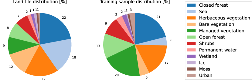
Figure 1: LULC distribution of the training samples in comparison to all land tiles.

Our sampling approach aimed at creating a high-quality dataset representing diverse land use and ecosystems for robust model training and validation, while minimizing cloud and missing data issues. We obtained this with the following steps. First, we began by calculating the proportion of LULC classes and ecoregions for each HLS tile using the Copernicus Land Cover 100m [7] and RESOLVE Ecoregions [8] labels. Second, after merging the twelve closed and open forest classes into two classes, we sampled 100 tiles per LULC class from the 500 tiles with the highest class proportion. Urban areas are upsampled by selecting 1,000 tiles that cover about 60% of the global urban areas. Additionally, we included 1,000 tiles with a high LULC class entropy to capture heterogeneous landscapes. Next, we ensured that the 846 ecoregions were represented if the size of the region allowed for it. In total, 712 ecoregions are present in three or more tiles, while 68 are not specifically included due to limited area coverage. Using a 95%-5% train-validation split, this process resulted in 3,156 train and 168 validation tiles. 133 of these tiles are missing in the final dataset due to quality issues or insufficient data coverage, e.g., in Greenland and Antarctica. The LULC distribution of the final dataset is visualized in Figure 1, clearly showing that sea and bare vegetation (desert) are down-sampled compared to all 18k HLS land tiles. Because we up-sample build-up areas, managed vegetation is also over-represented due to the geographical proximity.

Once ensured that we identified a diversified and representative set of tiles, the next phase of our dataset preparation aimed at optimizing both temporal and spatial coverage in sampling individual patches from the selected HLS tile ids (i.e. the actual satellite images used in the pretraining). This was particularly important because it enabled Prithvi-EO-2.0 to learn about seasonality and changes happening over a longer period of time. To achieve this, we aimed at building temporal sequences of four timestamps, with time difference between consecutive timestamps of one to six months and HLS data considered between 2014 and 2023.

The sequences were iteratively sampled from the selected HLS tiles until all candidates were processed or 1,500 samples per tile are reached (250 for validation tiles). Then, the sequences were split into non-overlapping 256 $\times$ 256 patches with four timestamps. We dropped all samples that include more than 1% of missing value pixels in any band or more than 20% of cloudy pixels using the HLS Fmask. The missing value pixels were filled with nearest interpolation. We ensured that each patch area has not more than ten samples and randomly down-sampled otherwise to not over-represent cloud-free areas and ensure spatial diversity (maximum two samples per area for validation). It is noteworthy that some areas can be more often present due to overlapping HLS tiles. Finally, all training samples that spatially overlap any validation area were dropped.

This patch-sampling strategy enabled us to maintain high data quality while ensuring a comprehensive representation of different temporal and spatial contexts in the dataset.

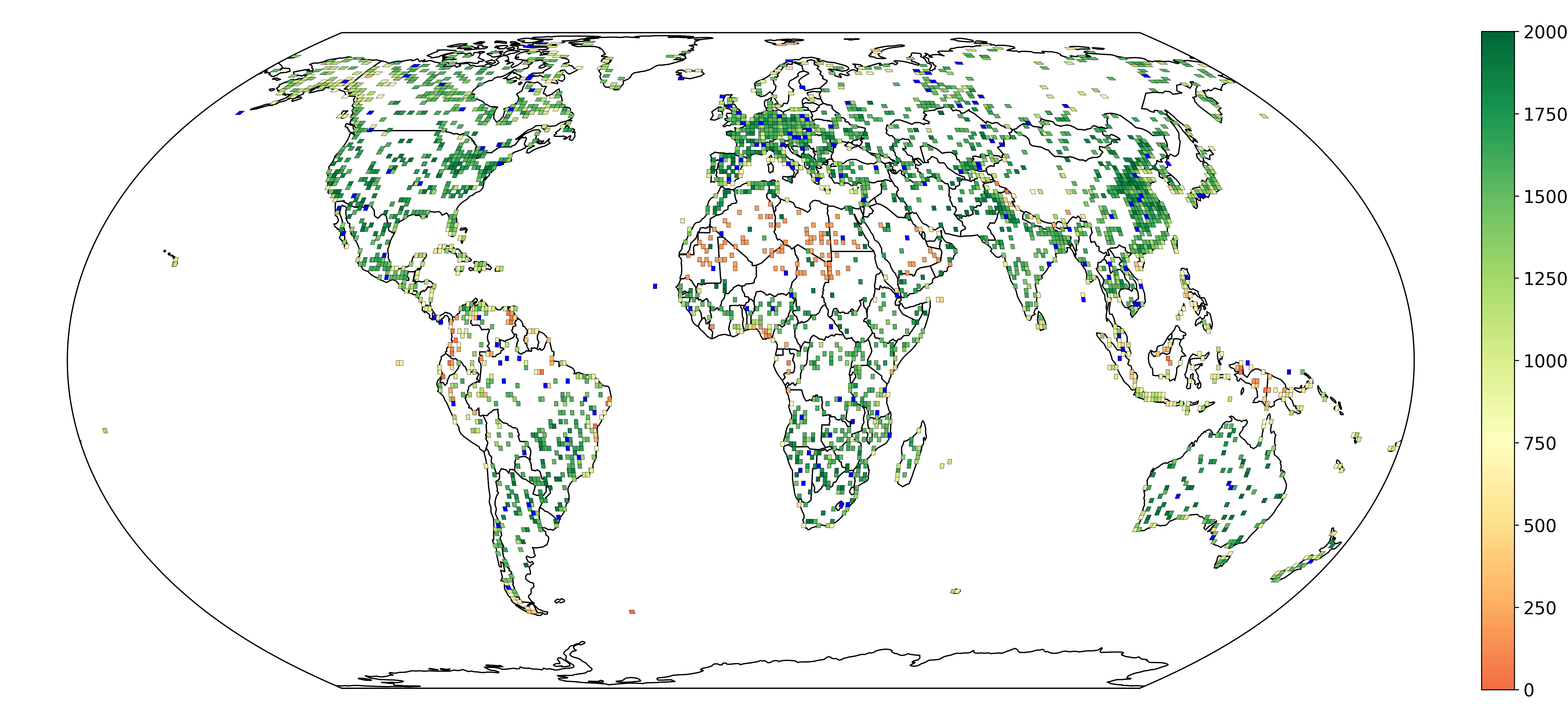
Figure 2: Global HLS dataset distribution visualized on a tile-level. The number of training samples are color-coded in orange to green while validation tiles are visualized in blue.

After preliminary pretraining experiments, we applied additional filtering to address data quality issues and maintain stable training conditions. Particularly, HLS tiles from central Greenland with persistent quality issues were removed from the dataset. We also sub-sampled full sea and desert regions due to their very low or high reflectance values to 10% to improve pretraining stability and avoid over-representation of homogeneous areas. Sea samples were filtered using the Fmask, while desert samples were reduced on a tile level. These filtering steps helped ensure that the dataset remained balanced, with a focus on diverse and representative land cover types, thereby supporting reliable model training and evaluation. The resulting pretraining dataset includes 4.2M training and 46k validation samples, which are visualized in Figure 2.

3 Pretraining and Model architecture

The pretraining process of our foundation model is based on the masked autoencoder (MAE) approach [9], a self-supervised learning method widely used and extended for different data types, including video [10] and multi-spectral images [11, 12]. The MAE reconstructs masked images using an asymmetric encoder-decoder architecture with a Vision Transformer (ViT) backbone. In detail, each input image is divided into non-overlapping patches of the same size and the ViT encoder embeds the patches using a linear projection with added 2D sin/cos positional embeddings. A subset of the patches is randomly masked and only the unmasked tokens are processed by the series of Transformer blocks of the encoder [9]. The decoder receives the encoded visible patches and mask tokens, which are learned vectors representing a missing token to be predicted. Positional embeddings are added to the full set of tokens and sent to the decoder’s series of transformer blocks to perform the image reconstruction task [9]. The loss function is the mean squared error (MSE) between the masked and predicted tokens in the pixel space [9].

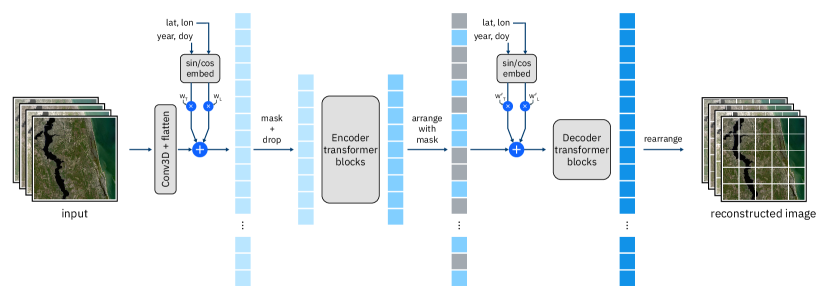
Figure 3: Prithvi architecture and general pretraining framework.

Figure 3 shows the overall MAE structure for pretraining Prithvi, which modifies the original MAE in two ways. First, we replaced the 2D patch embeddings and 2D positional embeddings with 3D versions to support inputs with spatiotemporal characteristics, i.e., a sequence of $T$ images of size $(H,W)$. Following approaches to adapt MAE to video processing [10, 13], our 3D patch embeddings consist of a 3D convolutional layer, dividing the 3D input into non-overlapping cubes of size $(t,h,w)$ for time, height, and width dimensions, respectively. Unlike videos, satellite data can be acquired at non-regular and relatively low frequency in time (days), so we set $t=1$ in our models. For the 3D positional encodings, we first generate 1D sin/cos encodings individually for time, height, and width dimensions and then combine them together into a single, 3D positional encoding.

Second, we considered metadata on geolocation (center latitude and longitude) and date (year and day-of-year ranging 1-365) in pretraining. The model receives time and location information for each sample and encodes them independently using 2D sin/cos encoding. They are added to the embedded tokens via a weighted sum with learned weights: one for time and one for location (see Figure 3). This means that we let the model learn how the metadata should be added to the embedded tokens. Since this metadata is often not available, we decided to include it not as additional inputs in patch embeddings, but as a simple bias, similar to the idea of positional encodings. For the same reason, we also added a drop mechanism during pretraining that randomly drops the geolocation and/or the temporal data to help the model learn how to handle the absence of this information.

Based on the above pretraining routine and architecture, we developed Prithvi-EO-2.0 in two sizes, 300M and 600M, based on ViT-L and ViT-H, respectively. We trained both versions with (Prithvi-EO-2.0-$\ast$-TL) and without (Prithvi-EO-2.0-$\ast$) temporal and location information. The models were trained for 400 epochs; the 300M models were trained on 80 GPUs (utilizing $\sim$21.000 GPU-hours for the full training), while the 600M models were on 240 GPUs (utilizing $\sim$58.000 GPU-hours for the full training). The local batch size (i.e., the batch size per GPU) for ViT-L was 48, and for ViT-H, was 16 to accommodate the larger model; a global batch size (i.e., the local batch size multiplied by the number of utilized GPUs) of 3,840 is then effectively used for all models. The weight decay was set to 0.05, and we used a cosine scheduler with a maximum learning rate of 5e-4, linear warmup for 40 epochs starting from a learning rate of 1e-6. For models with temporal and location data, we set the drop probability to 0.1. As described in section 2, the training samples have shape $4\times 256\times 256$ for time, height, and width, respectively, and we used random crop (final input shape is $4\times 224\times 224$) and random horizontal flips as data augmentation. Data parallelism in HPC systems is essential for efficiently handling large-scale remote sensing data required for training deep learning models [14]. By distributing the data across multiple GPUs, HPC systems can significantly reduce training time while maintaining accuracy. PyTorch DDP was used to scale the model pretraining. The models were pretrained on the Booster partition of the JUWELS (Jülich Wizard for European Leadership Science) supercomputer [15] hosted at JSC, which features 936 compute nodes, each equipped with 4 NVIDIA A100 GPUs.

4 Benchmarking and Downstream Tasks

There are two key aspects when evaluating the usefulness of a foundation model. First, it is to assess how the new foundation model compares to published competitors. This is done by benchmarking performance on an agreed set of tasks, following a rigorous protocol that allows for fair comparability and reproducibility. Second, the use the new foundation model in real-world downstream tasks and applications, implemented directly by subject matter experts (SMEs). In this case, the SMEs compare the foundation model to the state-of-the-art in their domain to assess whether there is any increase in performance.

These two activities are usually disjoint, and, to the best of our knowledge, never done and presented before as part of a holistic evaluation of a new model in EO and remote sensing. This usually does not happen because the researchers developing new foundation models usually come from an AI and computer science background, while the ones more interested in real-world scientific applications come more from a traditional remote sensing and earth observation background.

In our research, we went beyond these limitations and not only carried out the most in-depth benchmarking evaluation of a new EO model to date, but we also involved SMEs with different expertise throughout the design, training and evaluation of our model. As a matter of fact, SMEs informed design choices of our pretraining dataset, model architecture and evaluation, with novel real-world downstream tasks.

To make this possible, we addressed another key issue with the majority of EO foundation models published and released over the last few years. Particularly, it is common practice to release the model weights and architecture in places like Hugging Face and Github, however very rarely there are instructions on how to adapt the model to different applications or even a code base to easily fine-tune the model for new downstream tasks. Therefore, we onboarded Prithvi-EO-2.0 on TerraTorch, a PyTorch lightning and TorchGeo powered fine-tuning toolkit for Earth Observation foundation models that, once a model is onboarded, allows easy customization to classification, multi-label classification, semantic segmentation, and regression tasks.

In the next section, details on the Benchmarking and Downstream Tasks applications are reported.

4.1 Benchmarking

We used the most popular and rigorous benchmark framework available for Earth Observation foundation models: GEO-Bench [5]. GEO-Bench presents two key characteristics. First, it includes a carefully collected list of 6 classification and 6 semantic segmentation datasets for different resolutions and domains (see Table 1 and Figure 4). Second, it established a protocol that allows to compare different models fairly and reproducibly. This starts with hyperparameter tuning, where each model is allowed a budget of tries, 10 in our study, on each dataset. Then, the best hyperparameters found for each dataset on the validation set are used for repeated experiments (N=10) on each dataset with different seeds. This allows to account for randomness that is present when training AI models, and more confidently compare results.

Table 1: Characteristics of GEO-Bench datasets [5].

Classification
Name	Image Size	# Classes	Train	Val	Test	# Bands	Sensors
m-bigeartnet	120 $\times$ 120	43	20,000	1,000	1,000	12	Sentinel-2
m-so2sat	32 $\times$ 32	17	19,992	986	986	18	Sentinel-2 + Sentinel-1
m-brick-kiln	64 $\times$ 64	2	15,063	999	999	13	Sentinel-2
m-forestnet	332 $\times$ 332	12	6,464	989	993	6	Landsat-8
m-eurosat	64 $\times$ 64	10	2,000	1,000	1,000	13	Sentinel-2
m-pv4ger	320 $\times$ 320	2	11,814	999	999	3	RGB
Segmentation
Name	Image Size	# Classes	Train	Val	Test	# Bands	Sensors
m-pv4ger-seg	320 $\times$ 320	2	3,000	403	403	3	RGB
m-chesapeake-landcover	256 $\times$ 256	7	3,000	1,000	1,000	4	RGBN
m-cashew-plantation	256 $\times$ 256	7	1,350	400	50	13	Sentinel-2
m-SA-crop-type	256 $\times$ 256	10	3,000	1,000	1,000	13	Sentinel-2
m-nz-cattle	500 $\times$ 500	2	524	66	65	3	RGB
m-NeonTree	400 $\times$ 400	2	270	94	93	5	RGB + Hyperspectral + Elevation

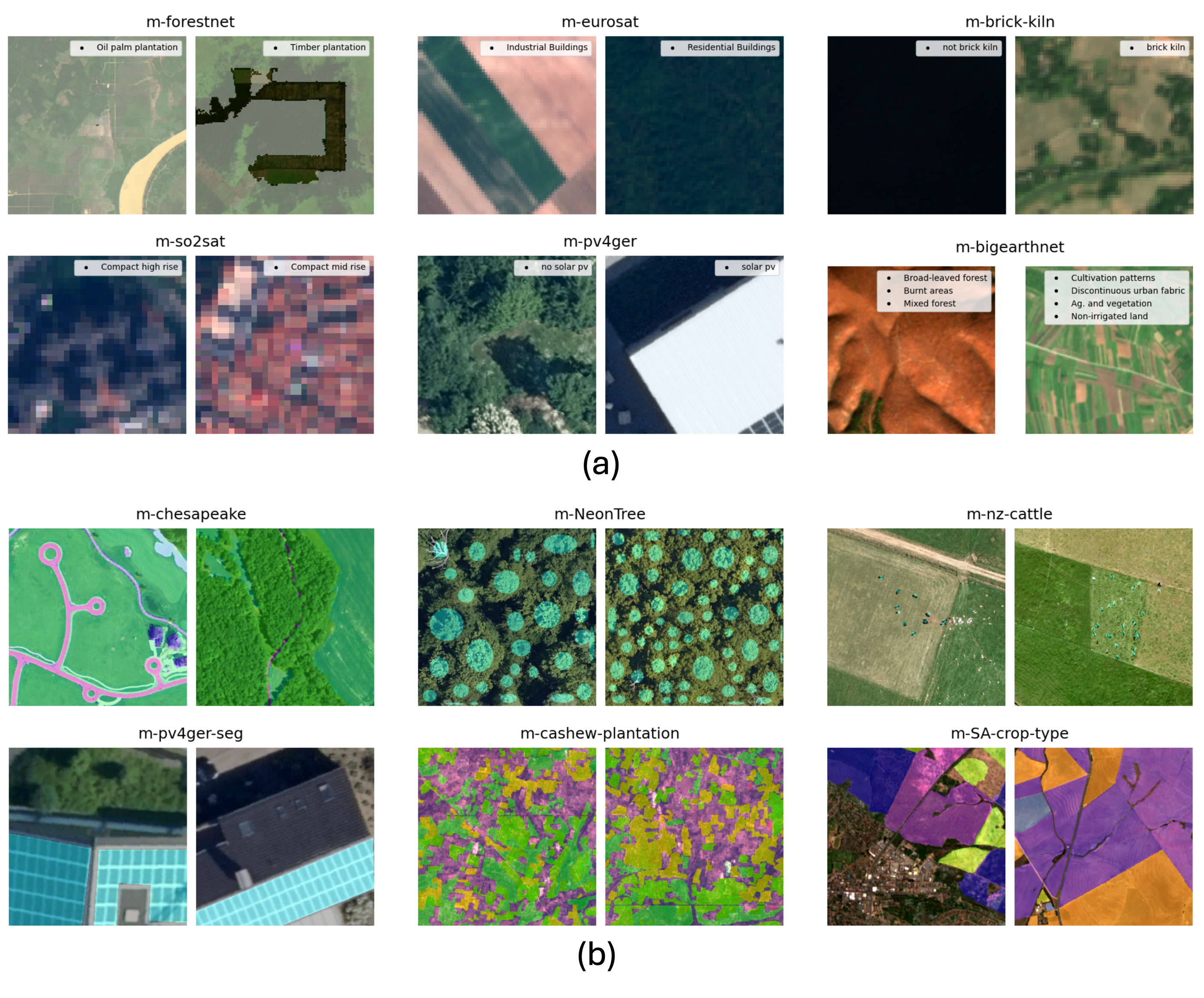
Figure 4: Examples of images and labels for the GEO-Bench datasets [5].

In our experiments, we onboarded all GEO-Bench datasets in TerraTorch. We then used its companion library TerraTorch-iterate (soon to be open sourced) to perform the hyperparameter tuning search via Bayesian Optimization in Optuna , as well as the repeated experiments. We compare Prithvi-EO-2.0 against six of the most popular and performant EO foundation models recently released (see Table 2), as well as the earlier version of Prithvi trained on the US only released last year [4]. For classification tasks, all models were paired with a linear layer, while we used a U-Net architecture [16] for ResNets and UPerNet [17] decoder for transformer-based architectures, which represent the most adopted choices for these types of architectures. Hyperparameter tuning was done across the same search space that included learning rate, decoder depth, and weight decay. For comparability, batch size was fixed to a reasonable value for each dataset for all models. Finally, in our experiments, we only used the optical sensors for each dataset, and for each model the bands it was pretrained on, with images that were all resized to 224 $\times$ 224 across all datasets.

Table 2: Comparison of characteristics of the various Geospatial Foundation Models compared to Prithvi-EO-2.0: number of parameters (# Param.), pretraining technique (Technique) and the data used in pretraining (Data), its resolution (Res.), number of samples (N), and number of time steps in a sample (T). Characteristics reported for the Satlas model pretrained on Sentinel-2 downstream tasks. Sample size of pretraining dataset (i.e. N column) is estimated when not clearly reported.

Model [Ref]	Type	# Param.	Technique	Sensors	Res.	N	T
MOCO [18]	ResNet50	25M	Contrastive learning	Sentinel-2	10m	1M	1
DINO [18]	ResNet50	25M	Contrastive learning	Sentinel-2	10m	1M	1
DeCUR [19]	ResNet50	25M	Contrastive learning	Sentinel-2	10m	1M	1
ScaleMAE [12]	ViT	300M	MAE	RGB	0.1-30m	360k	1
DOFA [20]	ViT	300M	MAE	NAIP Sentinel-2 Sentinel-1 EnMap Gaofen Landsat	1-30m	8M	1
Satlas [21]	Swin	100M	Supervised	Sentinel-2	10m	NA	1
Prithvi-EO-1.0 [4]	ViT	100M	MAE	HLS	30m	250k	3
Prithvi-EO-2.0	ViT	300M, 600M	MAE	HLS	30m	4.2M	4

Results of benchmarking are shown in Figures 6, 5 and 7. Figure 6 shows the average performance across the classification and segmentation datasets, while Figure 5 depicts the overall performance across all 12 datasets. These figures highlight that, for the classification tasks, DOFA [20] comes first, with Prithvi-EO-2.0-600M-TL close second and Prithvi-EO-2.0-600M third. For segmentation Prithvi-EO-2.0-600M-TL and Prithvi-EO-1.0-600M top the leaderboard with some margin on DeCUR [19] and DINO [18] ResNets. Overall, Prithvi-EO-2.0-600M-TL and Prithvi-EO-2.0-600M obtained the best combined performance across all 12 datasets. Note that in this case we are combining different metrics for different tasks (i.e., overall accuracy for classification and mean Jaccard Index for segmentation). However, such metrics are all between 0 and 1 and models are treated equally. Therefore, we believe this procedure is appropriate to get an overall performance picture across GEO-Bench datasets.

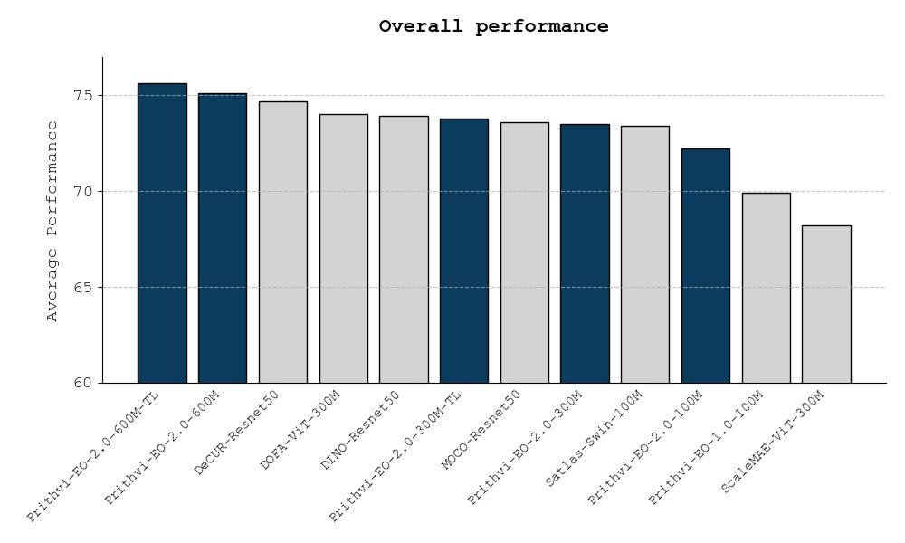
Figure 5: Overall average performance across all GEO-Bench datasets.

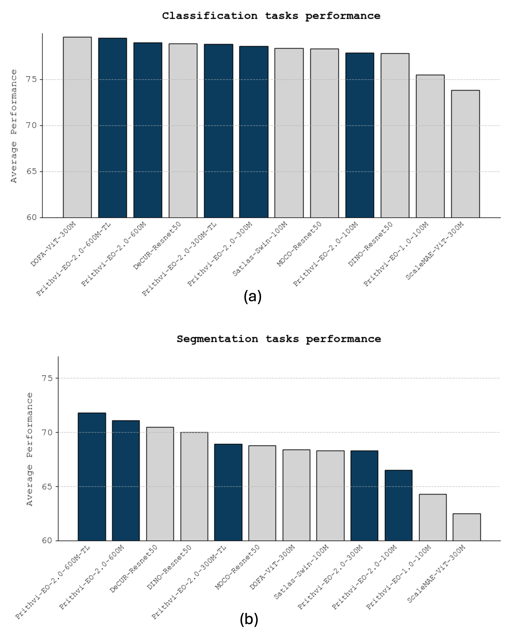
Figure 6: Averages for datasets over GEO-Bench classification (Overall accuracy) and segmentation (mean Jaccard Index) datasets.

Figures 5 and 6 are important to get an overall picture, while Figure 7 gives a more detailed view on the distribution of model’s performance across different datasets. Overall, it is interesting to see that some datasets carry very little insights to differentiate models, as performance is generally extremely high and condensed (e.g., m-brik-klin or m-pv4ger). For the other datasets, Prithvi-EO-2.0-600M-TL and Prithvi-EO-2.0-600M a the best performer in four out of six tasks targeting medium resolution (i.e. S2 at 10m), with tasks like m-bigearthnet and m-SA-crop-type classification that showed better performance by all Prithvi-EO-2.0-600M and Prithvi-EO-2.0-300M versions when compared to the other models. This is particularly interesting because these tasks focus on earth observation applications like land use classification using the CORINE Land Cover [22], which has strong focus on environmental monitoring categories (e.g. agriculture- and forest-related especially), and crop classification, which presents strong seasonality. These are exactly the type of domains that we targeted when crafting our multi-temporal global dataset, and these results suggest the model has learned relevant features to be highly performant on them.

Overall, beyond comparing against other models, there are three noteworthy points. First, the comparison between Prithvi-EO-2.0-100M and Prithvi-EO-1.0-100M, which are the same exact architecture and were just pretrained on different datasets, clearly shows the benefits introduced by our bigger global dataset. In fact, for the same size model and architecture there is a 3% improvement on the overall GEO-Bench score, with differences that are even larger for some of the tasks. Second, increasing the size of our models helped, as consistently larger Prithvi-EO-2.0 models performed better. Third, even though in GEO-Bench not all datasets contain temporal and location information, the models with temporal and location embeddings performed better overall. Finally, Prithvi-EO-2.0 also performed well on high-resolution tasks, despite pretraining included only data at a 30m resolution. This shows the versatility of our model towards more computer-vision-like applications such as tracking cattles on a field or identifying tree crowns from drone imagery.

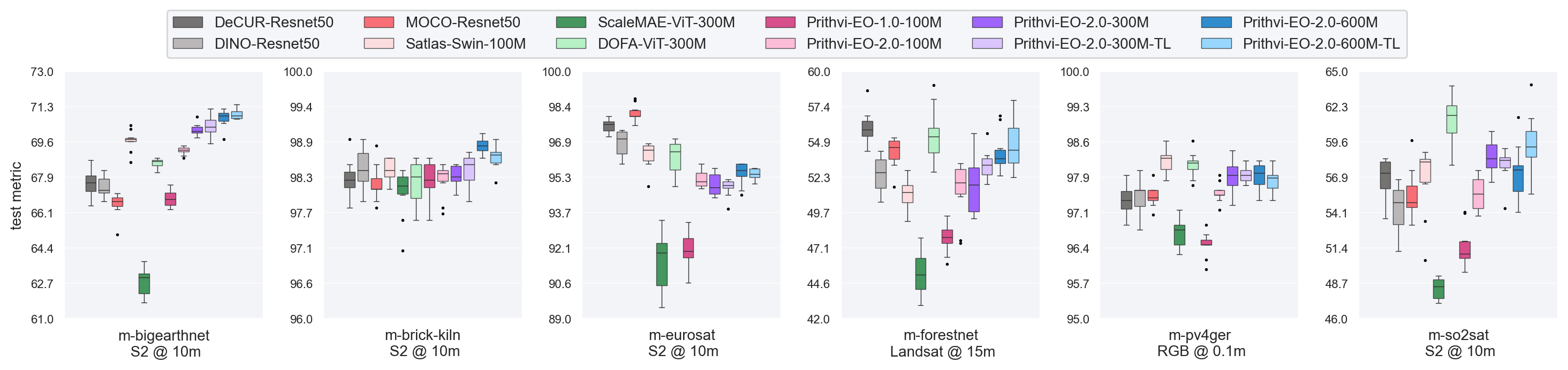
(a)

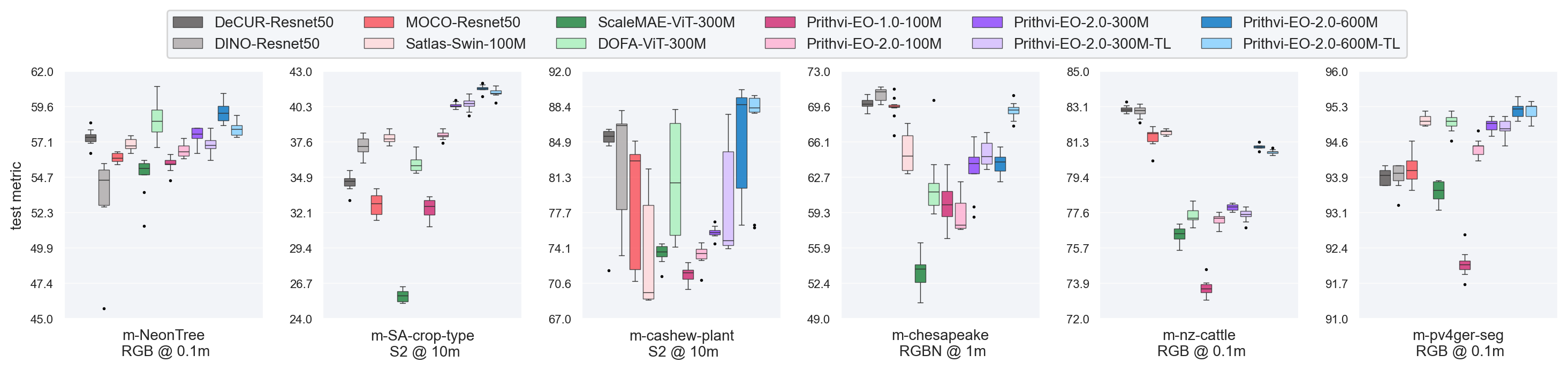
(b)

Figure 7: Distribution of performance across all models for classification (a) and segmentation (b) GEO-Bench [5] tasks in terms of overall accuracy and mean IoU, respectively. At the bottom of each graph, dataset input sensor and resolution.

4.2 Downstream tasks

This section presents real-world use cases of the adoption of the Prithvi-EO-2.0 by SMEs. As already mentioned, to make this process more accessible and encourage the community to adopt the model, the Prithvi-EO-2.0 models were onboarded on TerraTorch and paired with example code for fine-tuning the model. Each of the following subsections includes one complete use case, depicting the dataset that was used, methodology, and results compared to state-of-the-art. It is noteworthy that, considering the different background and practices in different domains, approaches adopted in each subsection will differ. However, this reinforces the concept of testing the model into the wild, in many and different ways.

We clustered the downstream tasks in three main areas: disaster response, land use and crop mapping, and multi-modal ecosystem dynamics monitoring. A full list can be found in Table 3

Table 3: Downstream tasks characteristics. T: Number of timestamps.

Domain	Task	Dataset size	T	Sensors
Disaster response	Flood detection	446 (448$\times$448)	1	S2
	Wildfire scar detection	805 (448$\times$448)	1	HLS
	Burn scar intensity	5,692 (32$\times$32)	1	HLS
	Landslide detection	3,799 (224$\times$224)	1	S2
Land cover and crop	Segmentation (US)	5,000 (224$\times$224)	3	HLS
	Classification (EU)	335,125 (64$\times$64)	up-to-12	S2
Ecosystem dynamics	Gross primary product	975 (50$\times$50)	1	HLS + MERRA2
	Above Ground Biomass	3,400 (256$\times$256)	4	S2+S1

4.2.1 Disaster response

Flood Mapping

Sen1Floods11 [23] is a surface water data set including labels for water and land, and related Sentinel-1 and Sentinel-2 imagery. The dataset consists of 446 $512\times 512$ chips covering 14 biomes, 357 ecoregions, and 6 continents of the world across 11 flood events between 2018 and 2020. The dataset and a reference training and evaluation code are available on GitHub. This dataset was used for testing Prithvi-EO-1.0, where the model showed beyond-state-of-the-art performance [4]. Here, we make a comparison with the newer Prithvi-EO version.

The $512\times 512$ images were resized to $448\times$448 as $512\times 512$ is not divisible by the patch size of the 600M models ($14\times 14$), and we wanted to guarantee all models were trained and validated with the same images (no padding or cropping). To increase data variability, random vertical and horizontal flips were applied as part of the data augmentation process. The associated masks present two categories: 0 for land and 1 for water. For all models, we have used an UPerNet [17] head decoder and ran hyperparameter tuning with terratorch (10 trials, tuning weight decay and learning rate). Then, we repeated the training with the best validation hyperparameters 10 times with different seeds and reported results on the test set. The loss used was cross-entropy and the models ran for 50 epochs with early-stopping patience set to 20 epochs. We used the same six bands as in the pretraining set.

Table 4 shows the results of our experiments in the test set. Prithvi-EO-2.0 improves over its previous version. Given the unbalanced nature of this dataset, where the land class is predominant and very easy to identify, improvements are minimal on the average statistics. However, we can see a clear difference between Prithvi-EO-1.0-100M and Prithvi-EO-2.0-600M with temporal and location embeddings of 3.5 points on the IoU for the water class.

Table 4: Results on the sen1floods11 dataset.

Model	mIoU (std)	mF1 (std)	IoU water (std)
Prithvi-EO-1.0-100M	88.3 (0.3)	97.3 (0.1)	79.6 (0.5)
Prithvi-EO-2.0-300M	89.7 (0.3)	97.6 (0.1)	82.2 (0.6)
Prithvi-EO-2.0-300M-TL	90.0 (0.2)	97.7 (0.1)	82.6 (0.3)
Prithvi-EO-2.0-600M	89.9 (0.6)	97.6 (0.2)	82.5 (1.0)
Prithvi-EO-2.0-600M-TL	90.3 (0.3)	97.7 (0.1)	83.1 (0.5)

Wildfire Scar Mapping

The wildfire scars dataset contains shapefiles of both intentional and wildfires burning from 2018–2021 as described in [4]. This dataset was used for testing Prithvi-EO-1.0, where the model showed state-of-the-art performance [4]. Here, we make a comparison with the newer Prithvi-EO version.

Also in this case, the $512\times 512$ images were resized to $448\times 448$, as explained in the flood case. To increase data variability, random vertical and horizontal flips were applied as part of the data augmentation process along with random crop to $224\times 224$. The corresponding masks for this use case were 0 for unburnt areas and 1 for burnt areas. For all models we have used an UPerNet head decoder [17] and ran hyperparameter tuning with terratorch (10 trials, tuning weight decay and learning rate). Then, we repeated the training with the best validation hyperparameters 10 times with different seeds and reported results on the test set. The loss used was cross-entropy and the models ran for 50 epochs, with early-stopping patience set to 20 epochs.

Table 5 shows the performance of the models on the wildfire scar mapping test set. Similar trends to the flood detection downstream tasks can be observed, with the newer version of the model outperforming Prithvi-EO-1.0. Again, differences become more marked when focusing on the IoU for the wildfire scar class, where the difference between older version of the model and Prithvi-EO-2.0-600M with temporal and location embeddings is of 5.6 points.

Table 5: Results on the wildfire scar mapping dataset.

Model	mIoU (std)	mF1 (std)	IoU burn scar (std)
Prithvi-EO-1.0-100M	86.9 (0.8)	97.2 (0.2)	76.8 (1.4)
Prithvi-EO-2.0-300M	88.6 (0.5)	97.6 (0.1)	79.9 (0.8)
Prithvi-EO-2.0-300M-TL	89.3 (0.9)	97.8 (0.3)	81.1 (1.6)
Prithvi-EO-2.0-600M	90.5 (0.6)	98.1 (0.2)	83.2 (1.1)
Prithvi-EO-2.0-600M-TL	90.5 (0.7)	98.1 (0.2)	83.2 (1.1)

Burn Intensity Mapping

We collected burn scar intensity data using paired Harmonized Landsat and Sentinel-2 (HLS) imagery and burn scar intensity classifications from Burned Area Emergency Response [24], which evaluates fire impacts on vegetation, soil, and watershed functionality. BAER teams rapidly analyze post-fire conditions to stabilize affected landscapes and mitigate hazards. The dataset includes 5,692 TIFF files capturing spatial burn scar data and top-of-atmosphere (TOA) reflectance values across three temporal stages: pre-burn, during-burn, and post-burn from 2018 to 2023, over the western CONUS (126^o W to -104^o W and 32.5^o N to 48^o N). Burn scar intensity classifications, ranging from 0 (no burn) to 4 (high severity), were derived from burn severity analysis. The HLS imagery was carefully selected to match the temporal criteria for pre-fire and post-fire stages, ensuring that changes in burn intensity and reflectance values were accurately captured. Each fire event is represented by paired 224 $\times$ 224 pixel TIFF files: one for burn scar intensity and another for TOA reflectance across six spectral bands (Blue, Green, Red, NIR, SWIR 1, SWIR 2). The images were visually inspected to confirm burn scar visibility and cloud-free conditions. The dataset was further refined excluding entries with more than 25% missing or zero values, ensuring high-quality data for training machine learning models. This dataset was used to evaluate wildfire impacts, where the burn scar intensity data and HLS spectral information enabled the testing of advanced remote sensing models. The dataset’s design ensures reproducibility and usability for wildfire monitoring and environmental research.

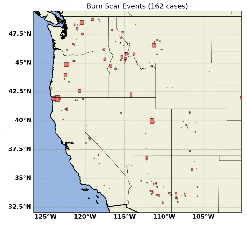
Figure 8: Locations of burn intensity dataset used in training, testing and validation.

Out of 5,692 images of size $32\times 32$ 80% was used for training and 20% for validating the Prithvi pretrained model for burn intensity mapping downstream application. The architecture for this task consisted of the Prithvi encoder, along with a decoder based on convolutional and upsampling layers. The target mask pixels were categorized into four burn classes, ranging from low to high intensity of burn scar. The model was trained for 150 epochs, with weighted cross-entropy used as the loss function. The results showed that the Prithvi-EO-2.0-300M model was comparable to the standard U-Net model in terms of mean IoU and mean F1 score. The small difference of performance in this case might be linked to the adoption of a much smaller patch than in pretraining, and the particular ability of U-Net to extract local level information. However, performance is generally low for all models, with the larger version of the models presenting overfitting in training curves.

Table 6: Results on the burn intensity dataset.

Model	mIoU	mF1	mAcc
U-Net	29.3	44.0	47.4
Prithvi-EO-2.0-300M	29.4	44.0	47.2
Prithvi-EO-2.0-600M	28.6	43.0	46.8

Landslide Detection

The Landslide4Sense (L4S) dataset [25] is a comprehensive benchmark for large-scale landslide detection research, utilizing multi-source satellite imagery to study landslide-affected areas globally from 2015 to 2021. It includes 14 data layers: Sentinel-2 multispectral bands (B1–B12), a digital elevation model (DEM), and slope data from ALOS PALSAR [25]. All layers are resized to a resolution of 10m per pixel and labeled at the pixel level as landslide or non-landslide. The dataset is divided into training, validation, and test sets, covering diverse mountainous regions worldwide. The training data comes from four sites: Iburi-Tobu (Hokkaido), Kodagu (Karnataka), Rasuwa (Bagmati), and western Taitung County, comprising 3,799 image patches, each 128$\times$128 pixels in size. The validation and test sets include 245 and 800 image patches, respectively, each of size 128$\times$128 pixels.

To fine-tune the Prithvi-EO-2.0 models for landslide mapping task, we incorporated a decoder consisting of four deconvolutional layers, along with layer normalization and activation functions, to map the model outputs from embeddings back to the original input image size. A fully convolutional network (FCN) was then applied to project the output from the latent space to the corresponding class probabilities. For the Prithvi-EO-2.0-600M configuration, which uses a patch size of 14$\times$14, this decoder architecture does not allow for the perfect restoration of embeddings to the input image size. To address this issue, we added a bilinear interpolation layer following the FCN to resize the output and ensure it matches the original input image dimensions.

The models were fine-tuned using the data split described in the previous section on the L4S dataset. Six input bands—Blue, Green, Red, NIR, SWIR1, and SWIR2—were selected, aligning with the pretraining phase of the Prithvi model. The input images are up sampled into 224$\times$224 to match the configuration of Prithvi backbone. Data augmentation was applied by randomly flipping images both vertically and horizontally. The model was fine-tuned with two different loss functions: weighted cross-entropy (wCE) loss, with a weighted ratio of 2:8 for negative and positive pixels, and Lovasz loss [26]. Gradient descent was performed using the Adam optimizer with a learning rate of 1e-5. Additionally, a cosine learning rate scheduler with warm-up and restart [27] was utilized to enhance model convergence. The model was trained for 100 epochs with a batch size of 8, and the checkpoint with the lowest validation loss was selected for evaluation.

For a comparative study on the landslide mapping task, U-Net [28] and U-Net++ [29] were employed. These are popular and powerful models that have been used to support a wide range of environmental mapping tasks, including landslide mapping [30, 31, 32]. It is worth noting that this dataset was also used in the 2022 Landslide4Sense (L4S) competition, with several winning models reported by [31]. However, those models and results were based on customized training strategies, such as self-training using test data, pseudo-label refinement, and ensemble methods. In contrast, our study focuses on evaluating the performance of the foundation model, Prithvi-EO-2.0, on the L4S downstream task and comparing it with existing deep learning models under a standardized training protocol (e.g., consistent data splits, augmentation techniques, and training platforms) as discussed above to ensure a fair comparison.

Table 7: Model performance metrics on full training dataset (100% or 3799 images).

Model	Evaluation Dataset	Loss Function	mIoU	F1 Score	Precision	Recall	aAcc
U-Net  (ResNet50)	Test	wCE	70.4	59.7	56.2	63.6	98.4
U-Net++  (ResNet50)	Test	wCE	69.0	57.0	50.2	68.4	98.0
Prithvi-EO-2.0-600M	Test	Lovasz	71.3	60.7	57.1	64.7	98.4
Prithvi-EO-2.0-600M	Test	wCE	70.4	58.6	51.1	68.6	98.2

The fine-tuned models were evaluated using three primary metrics: 1) mean Intersection over Union (mIoU), which calculates the average IoU between predicted and ground truth regions for each class; 2) F1 score, which balances precision and recall to assess the model’s overall accuracy; and 3) pixel accuracy (aAcc), which measures the percentage of correctly classified pixels across all classes. The results are presented in Table 7, where only the configurations yielding the best performance for each model are shown. From the results, Prithvi 300M, trained with Lovasz loss, outperformed both U-Net models in terms of mIoU, F1 score, and precision by a noticeable margin. Prithvi-EO-2.0-600M, trained with weighted cross-entropy loss, exhibited a slightly lower mIoU of 70.4% and an F1 score of 58.6%, but achieved a higher recall than Prithvi-EO-2.0-300M. In summary, Prithvi-EO-2.0-300M demonstrated the best overall performance based on mIoU and F1 score, while Prithvi-EO-2.0-600M showed a higher recall but sacrificed precision.

Table 8: Model performance metrics on a small training dataset (2.5% or 100 images).

Model	Evaluation Dataset	Loss Function	mIoU	F1 Score	Precision	Recall	aAcc
U-Net  (ResNet50)	Test	wCE	65.1	49.1	41.7	60.0	97.7
U-Net++  (ResNet50)	Test	wCE	65.5	50.2	40.9	65.2	97.5
Prithvi 300M	Test	Lovasz	66.6	49.8	56.8	44.4	98.3
Prithvi 600M	Test	wCE	67.1	49.1	54.3	44.8	98.3

The models were also fine-tuned on a significantly smaller subset of the training dataset to assess their generalizability. Table 8 shows the evaluation results for models trained on only 100 images (approximately 2.5% of the full training dataset). As expected, training on such a small subset led to performance degradation across all models, but the degree of decline varied. Both U-Net and Prithvi-EO-2.0-300M experienced a noticeable performance drop. For instance, U-Net’s mIoU decreased from 70.4% to 65.1%, and its F1 score fell from 59.7 to 49.1. Prithvi-EO-2.0-300M also observed a drop, though it still demonstrated the best precision and nearly matched the best F1 score. In contrast, Prithvi-EO-2.0-600M and U-Net++ exhibited a more moderate performance decline. Notably, Prithvi-EO-2.0-600M showed a smaller reduction in mIoU, from 70.4% to 67.1%. This model was less affected by the smaller dataset, likely due to its larger size and specialized pretraining, which enhanced its ability to generalize with limited data. Overall, Prithvi-EO-2.0-600M exhibits the highest level of resilience to data reduction among all comparative models, maintaining strong performance.

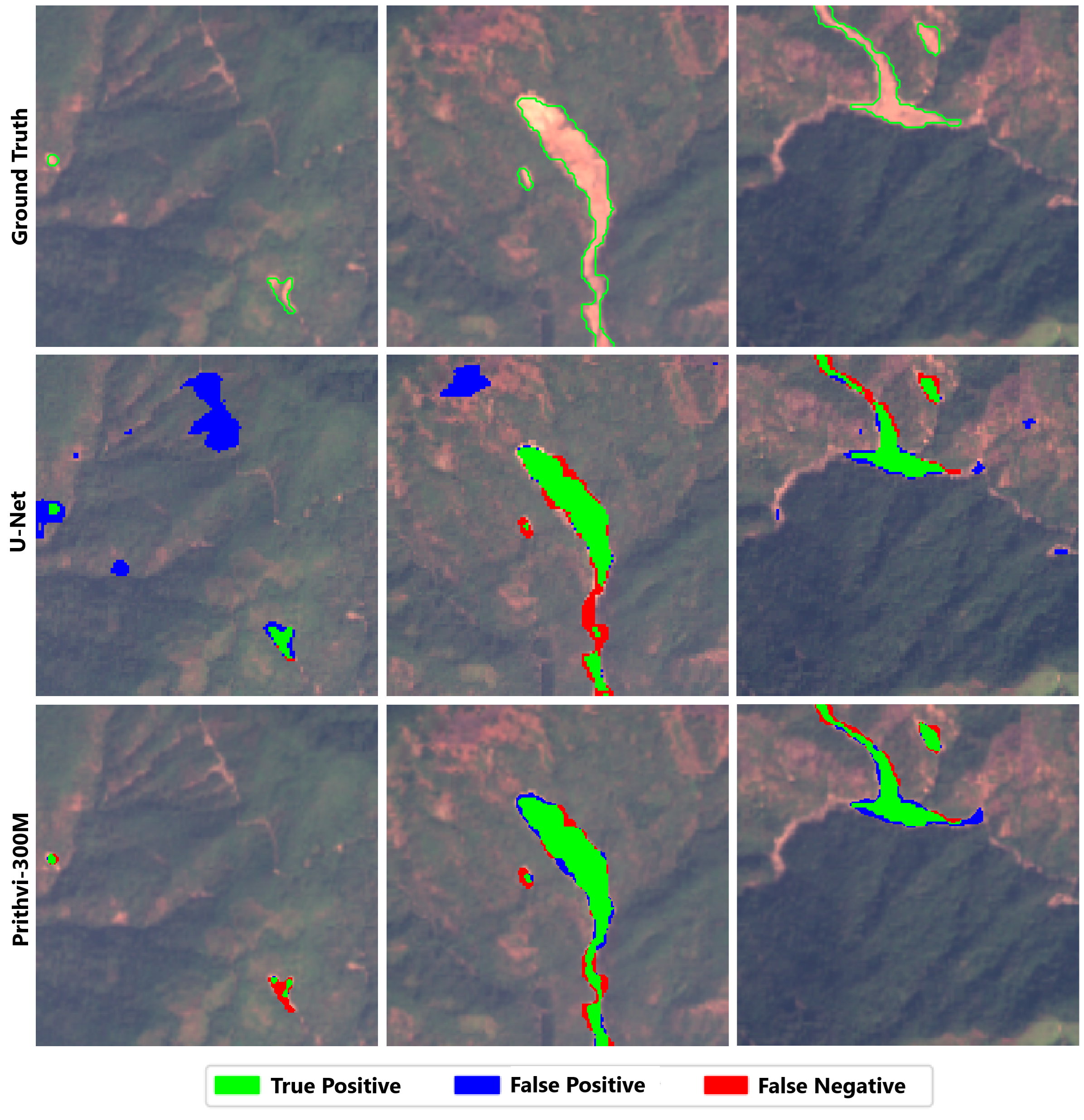
Figure 9: Example testing results to illustrate models’ performance on the full training dataset.

We also selected three pairs of segmentation results from the top-performing Prithvi and U-Net models to conduct a visual comparative analysis of segmentation performance, using sensitivity and specificity statistics. Figure 9 illustrates the results of U-Net and Prithvi-EO-2.0-300M, both fine-tuned on the full training dataset, while Figure 10 shows the results for U-Net++ and Prithvi-EO-2.0-600M, fine-tuned on a smaller subset of 100 images.

In Figure 9, Prithvi-EO-2.0-300M exhibits a more conservative detection approach, with fewer False Positives (blue) but a broader coverage of True Positives (green), capturing the target regions with higher accuracy. However, it shows a slightly higher incidence of False Negatives (red) in some cases. In contrast, U-Net results in more False Positives, leading to a lower accuracy and an overall F-1 score. This indicates that Prithvi-EO-2.0-300M prioritizes detection accuracy by effectively reducing False Positives. While this approach may potentially sacrifice recall in certain areas, it achieves the best prediction performance among all models compared.

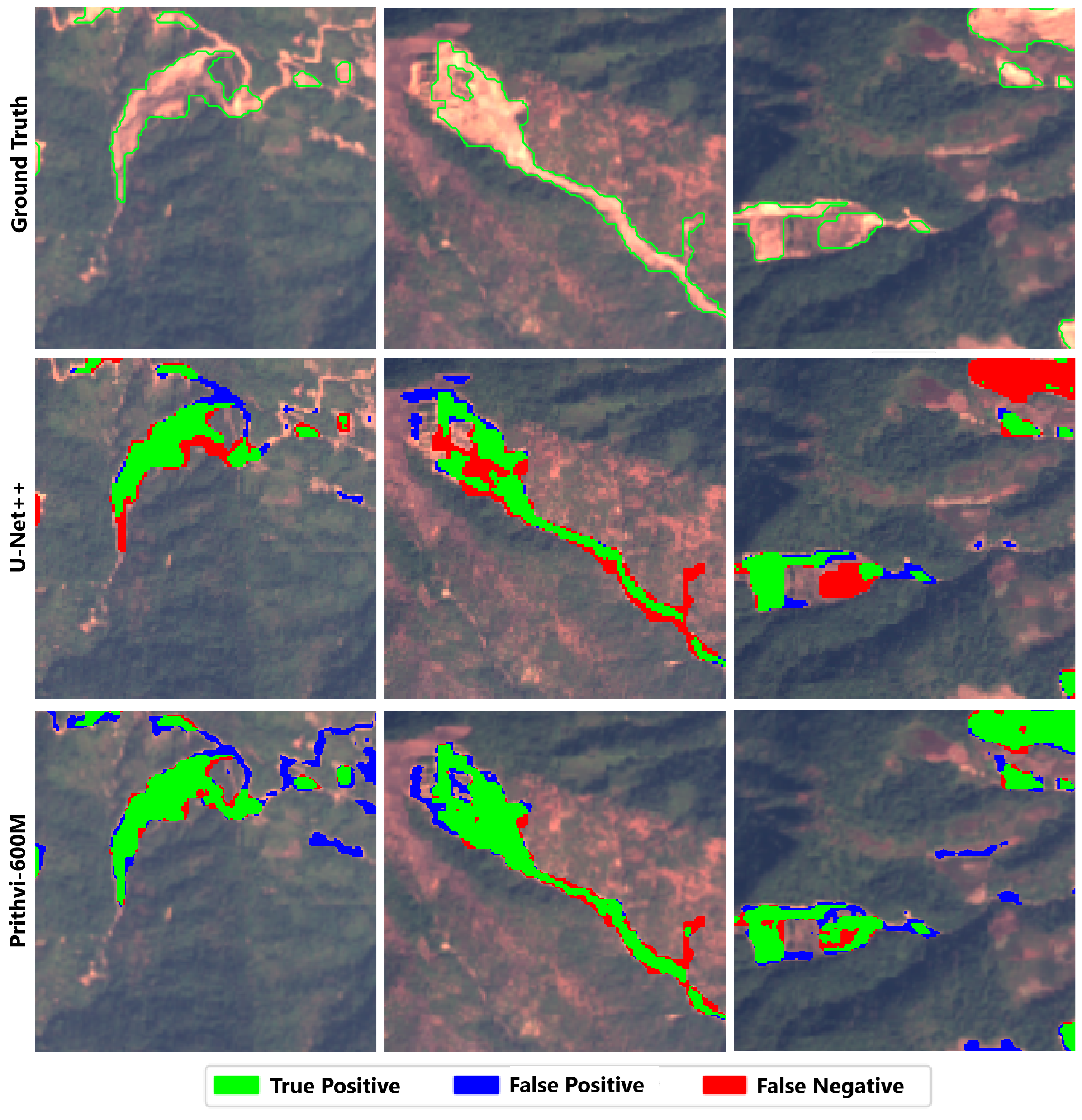
Figure 10: Example testing results to illustrate models’ performance on a small training dataset (2.5% or 100 images).

Figure 10 reveals a different pattern in the segmentation results of U-Net++ and Prithvi-EO-2.0-600M. U-Net++ tends to produce more False Negatives, often missing parts of the target regions, while maintaining moderate levels of False Positives. Prithvi-EO-2.0-600M, however, shows a more balanced performance with broader True Positive coverage across the target regions, although it occasionally generates slightly more False Positives compared to U-Net++. This suggests that Prithvi-EO-2.0-600M leverages its enhanced model capacity to generalize effectively, even with limited training data, prioritizing sensitivity and reducing under-segmentation compared to U-Net++.

4.2.2 Land use and land cover mapping

Multi-Temporal Crop Segmentation in the United States

This dataset was used for testing Prithvi-EO-1.0, where the model showed state-of-the-art performance [4]. Here, we make a comparison with the newer Prithvi-EO version.

The $224\times 224$ images were used for both training and validation without cropping. To enhance data variability, random vertical and horizontal flips were applied as part of the data augmentation process. The corresponding masks were categorized into thirteen classes: 1) "Natural Vegetation", 2) "Forest", 3) "Corn", 4) "Soybeans", 5) "Wetlands", 6) "Developed/Barren", 7) "Open Water", 8) "Winter Wheat", 9) "Alfalfa", 10) "Fallow/Idle Cropland", 11) "Cotton", 12) "Sorghum", and 13) "Other".

All models were combined with a simple segmentation decoder consisting of convolutional and upsampling blocks, for fine-tuning on multi-crop segmentation. Weighted cross entropy was used as a loss function. The results show that the Prithvi-EO-1.0-100M, Prithvi-EO-2.0-300M, and Prithvi-EO-2.0-600M models outperform the U-Net model in terms of mean IoU, and mean accuracy. Among all the Prithvi models, the 600M variant achieved the best performance, with a mean IoU of $50.7\%$ and mean accuracy of $68.8\%$. The training was performed for 80 epochs.

Table 9: Results on the multitemporal crop segmentation dataset.

Model	mIoU	mAcc
U-Net	42.6	61.9
Prithvi-EO-1.0-100M	42.7	60.7
Prithvi-EO-2.0-300M	48.6	66.8
Prithvi-EO-2.0-600M	50.7	68.8

Multi-Temporal Land Cover and Crop Classification in Europe

Sen4Map [33] is a benchmark dataset designed for multitemporal land-cover and crop classification tasks with Sentinel-2 satellite data. Sen4Map comprises 335,125 time series of 64$\times$64 pixels multispectral patches, extracted from Sentinel-2 tiles and annotated with geolocated land-cover data collected through extensive in situ surveys using LUCAS points [34]. The dataset includes time-series of varying lengths from 2018, covering countries across the European Union. We utilized the monthly composites, feeding the models with time-series of length 12, in line with the original paper. The spatial resolution of the images in Sen4Map is natively 10 m or upsampled to 10 m from the native 20 m resolution, depending on the spectral band provided by Sentinel-2. Each image covers an area of 640 m $\times$ 640 m, which contrasts with our pretraining dataset, where the images are 224 $\times$ 224 pixels with a spatial resolution of 30 m, covering approximately 6720 m $\times$ 6720 m—over 100 times the area of the Sen4Map samples. This significant scale difference between the fine-tuning and pretraining datasets presents a noteworthy challenge during validation. The patch-processing methodology further compounds this challenge. In Sen4Map, the original 64 $\times$ 64-pixel patches are cropped down to smaller 15 × 15-pixel regions to focus on the images’ central pixels, centered around the available label from LUCAS. This ensures that classification is based solely on the area of interest while minimizing the influence of irrelevant spatial context. We adopted a similar setup to maintain a fair comparison. The cropped 15 $\times$ 15-pixel patches were upscaled to 224 $\times$ 224 pixels to align with the input requirements and reuse the patch embeddings of Prithvi. In addition to differences in spatial resolution and patch size, the datasets vary in the spectral bands. The pretraining dataset includes only six of the thirteen Sentinel-2 bands (Red, Green, Blue, Nir-Narrow, Swir1, and Swir2), while the Sen4Map dataset provides four additional bands (Nir-Broad and Red-Edge 1, 2, and 3), for a total of ten bands. These differences in spatial, spectral, and contextual characteristics add complexity to the model’s validation and fine-tuning process. We fine-tuned the original Prithvi-EO-1.0-100M model, Prithvi-EO-2.0-300M, and Prithvi-EO-2.0-600M, on different fractions of the Sen4Map training data. We compared them with the baseline ViViT used in Sen4Map, which was recreated to be trained from scratch on the fractions. In the land cover classification task, reported in Table 10, Prithvi-EO-2.0-600M demonstrates superior performance compared to all other models across all data fractions in terms of weighted-averaged F1 score. Table 11 depicts results on the crop type classification task, where Prithvi-EO-2.0-600M achieves performance comparable to Prithvi-EO-2.0-300M, showing marginally better results on two data fractions and slightly lower performance on three fractions; both models demonstrate superior performance compared to Prithvi-EO-1.0-100M and the baseline ViViT.

Table 10: Mean F1 score and std for the land cover classification, fine-tuning the models on fractions of the original dataset, compared to baseline ViViT [33].

Fraction	ViViT (Sen4Map)	Prithvi-EO- 1.0-100M	Prithvi-EO- 2.0-300M	Prithvi-EO- 2.0-600M
1.0	72.7 (0.3)	74.5 (0.3)	76.0 (0.3)	76.1 (0.2)
0.5	69.9 (0.4)	72.4 (0.4)	73.9 (0.4)	74.1 (0.3)
0.25	65.7 (0.7)	69.1 (0.5)	70.7 (0.6)	71.2 (0.5)
0.125	61.6 (0.5)	65.3 (0.5)	67.1 (1.1)	67.8 (1.4)
0.0625	55.0 (1.3)	59.4 (1.3)	61.2 (1.4)	62.3 (0.9)

Table 11: Mean F1 score and std for the crop type classification task, fine-tuning the models on fractions of the original dataset, compared to baseline ViViT [33].

Fraction	ViViT (Sen4Map)	Prithvi-EO- 1.0-100M	Prithvi-EO- 2.0-300M	Prithvi-EO- 2.0-600M
1.0	81.5 (0.3)	83.0 (0.3)	84.4 (0.2)	84.6 (0.2)
0.5	79.0 (0.3)	81.5 (0.2)	82.8 (0.2)	82.6 (0.2)
0.25	75.5 (0.4)	78.6 (0.4)	80.4 (0.4)	80.5 (0.3)
0.125	69.7 (1.0)	74.6 (0.7)	77.3 (0.4)	76.9 (0.5)
0.0625	64.5 (1.4)	70.5 (1.0)	72.2 (1.4)	70.8 (0.9)

4.2.3 Multi-modal Ecosystem Dynamics

Above Ground Biomass Estimation

Above Ground Biomass (AGB) is a crucial climate variable that encompasses all living biomass above the soil, essential for understanding land use changes and carbon inventories. Although direct measurement of AGB is challenging, remote sensing methods and machine learning techniques can be used to estimate it, providing comprehensive spatial and temporal data. The BioMassters dataset aimed to explore deep learning approaches for predicting yearly Above Ground Biomass (AGB) in Finnish forests using multi-modal, multi-temporal Sentinel-1 and Sentinel-2 satellite data from 2016 to 20212. The dataset comprises 11,462 AGB reference images, each paired with 12 months of corresponding satellite imagery, covering 2,560$\times$2,560-meter forest patches, with AGB measured in metric tonnes per pixel and derived from LiDAR data calibrated with in-situ measurements. The winning model from the data challenge is used as the benchmark for comparison with the Prithvi model. This model is based on a U-Net architecture with temporal attention encoding [35], using all 12 time steps and all 15 channels from Sentinel-1 and Sentinel-2 imagery as inputs for each yearly AGB prediction. The winning model achieved an RMSE of 27.49 on the holdout test set.

The dataset has been tailored for the Prithvi model by incorporating metadata for filtering, such as cloud coverage and corrupt values, while selecting specific Sentinel-2 bands that align with those used during pretraining. Additionally, the Radar Vegetation Index (RVI) from SAR data was included as an input, and the dataset was divided into 80% training and 20% validation sets for consistent experimental use. For testing, 4 time steps were chosen out of 12 based on the quality of the Sentinel-2 data—priority was given first to scenes with complete values with no blank areas, then to scenes with the lowest cloud cover. As targets cannot be filtered from the test set based on incomplete data, some Sentinel-2 inputs are low quality for the test set.

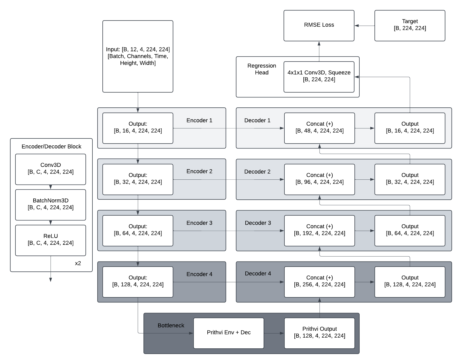
Figure 11: Model architecture for predicting AGBM on BioMassters Dataset using U-Net Prithvi.

The model architecture selected for training was a Prithvi-UNet hybrid with the pretrained Prithvi encoder and decoder as the bottleneck, shown in Figure 11. The channel-specific positional encoder is removed to allow the model to process inputs with a channel dimension of 128. No model weights were frozen during training.

Five experiments were conducted, each with random initialization of encoder-decoder weights. For training augmentation, random vertical and horizontal flipping, as well as random cropping from $256\times 256$ to $224\times 224$, were applied. For validation and testing, center cropping to $224\times 224$ was applied.

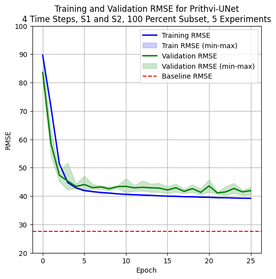
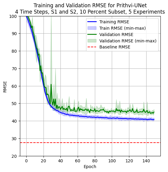
Figure 12: Training and validation loss of BioMassters Prithvi U-Net on the full filtered training set (left) and on random 10% subsets (right).

Training and validation loss on the filtered training subset are compared to the baseline model performance in Figure 12, which shows performance on both the full filtered training set and randomly sampled 10% subsets. For the full training set, all experiments converge to just above 40 RMSE on the validation set. Best performance is at Epoch 22, with 40.35 RMSE. For the 10% subsets, best performance is at Epoch 142, with 43.05 RMSE. For reference, the baseline model achieves 28.46 RMSE on an identical validation set.

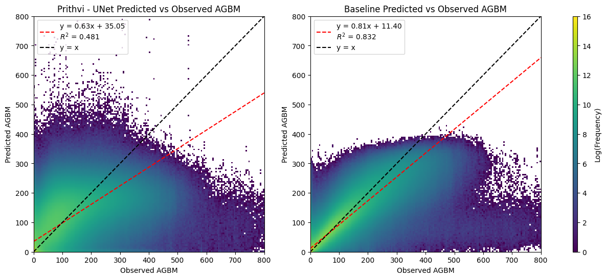
Figure 13: Comparison of Prithvi-UNet and Baseline AGBM predictions versus observed AGBM for all inputs in the test set. A log scale is used for visualization.

Figure 13 shows the $R^{2}$ score of the Prithvi-UNet model and the baseline model on all AGBM targets in the test dataset. The baseline model shows a tighter distribution around the identity line, as well as more accurate prediction of high AGBM values from $300-400$. However, both models underestimate higher AGBM values ($>400$). As the test set has more incomplete Sentinel-2 inputs, the performance of the Prithvi-UNet is negatively affected, as shown in 12

Table 12: Comparison of RMSE Metrics Across Models and Datasets

Metric	Prithvi-UNet 300M, Full Dataset	Prithvi-UNet 300M, 10% Subset	BioMassters Baseline
Validation Set RMSE	40.35	43.05	28.46
Test Set RMSE	54.51	56.05	27.49

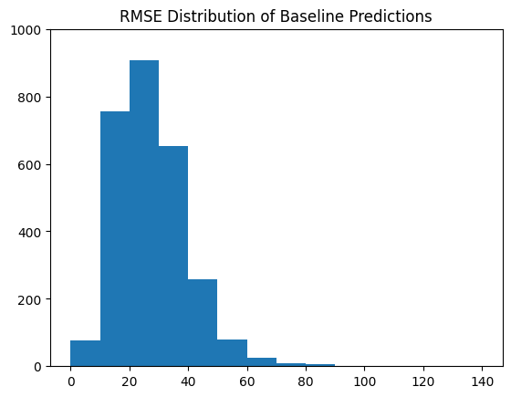
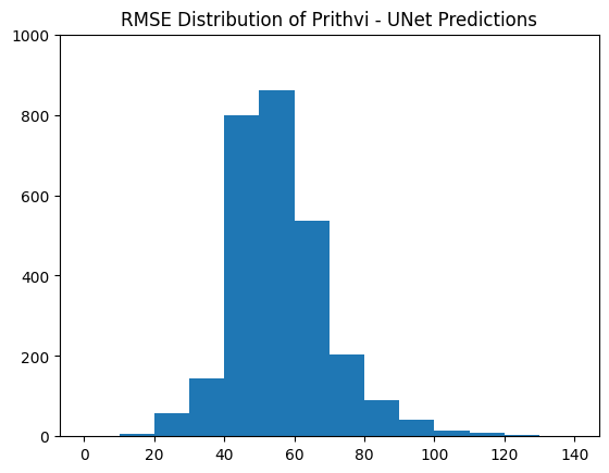
Figure 14: Histograms of RMSE between observed AGBM maps in the test set as compared to predicted AGBM maps from both the baseline model (left) and Prithvi-UNet (right).

Figure 14 shows the distribution of the RMSE of each predicted AGBM map as compared to the map of observed RMSE. While some scenes are challenging for both models, the baseline model shows lower RMSE values overall.

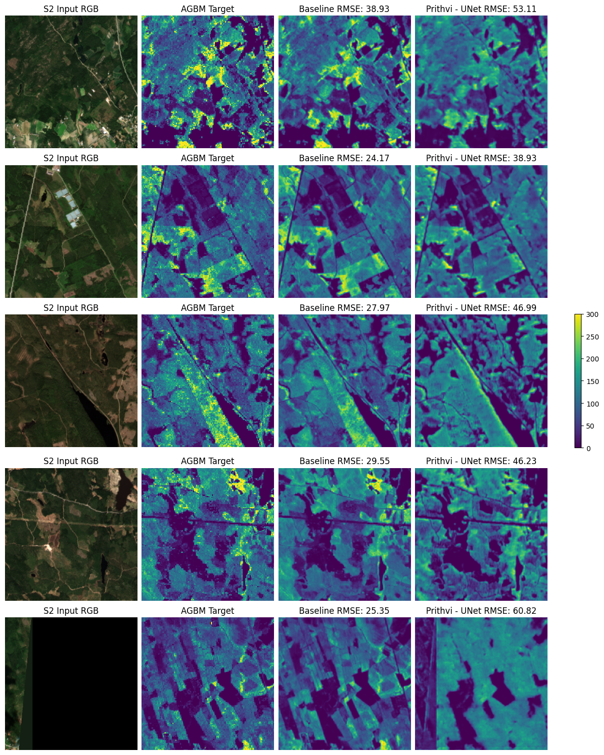
Figure 15: Comparison of Prithvi and Baseline prediction on 5 input and AGBM target pairs from the test set. Columns from Right to Left: RGB Visualization of Sentinel-2 scene from a single time step, Target AGBM, Baseline Model Prediction, and Prithvi-UNet Prediction. As high-quality Sentinel-2 data does not exist for all AGBM targets, some S2 inputs, such as that in row 5, are either obscured by clouds or contain partial data.

Qualitative observation of selected outputs in Figure 15 show that baseline outputs and Prithvi-UNet outputs are visually similar for some input scenes. Both models show predictions that are smoother than the observed AGBM values. Higher AGBM values appear to be predicted more accurately by the baseline model than by Prithvi-UNet. Additionally, the baseline model is better at handling cases in which Sentinel-2 data is low quality or unavailable for a given AGBM target.

The results of these experiments show that Prithvi is capable of adapting to multi-modal inputs, integrating both SAR and MSI imagery. However, for optimized results for this task more work is required.

Estimation of Gross Primary Productivity (GPP) at Globally Distributed Sites

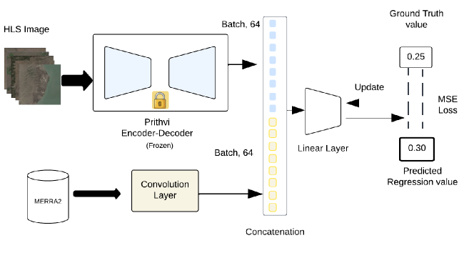
Figure 16: Workflow to fine-tune Prithvi for predicting GPP at flux observations sites. The approach consists of two branches, with the (frozen) Prithvi encoder deriving HLS embeddings which are transformed by a simple decoder, and a convolutional branch transforming MERRA-2 atmospheric and land surface variables. The HLS decoder and convolved MERRA-2 outputs are concatenated and trained to predict GPP with a linear layer.

Photosynthesis (Gross Primary Productivity (GPP)), the critical process converting solar radiation into energy and materials that sustain life, represents the largest global carbon cycle flux, yet remains challenging to quantify accurately without direct observation [36]. Data-driven approaches using machine learning to integrate satellite data with site-level information (e.g. from eddy covariance measurement networks [37]) provide diagnostic constraints on global GPP, complementing process-based models [38]. However, these approaches face challenges due to scale mismatches between in-situ measurements and satellite data, as well as generalization issues, which could potentially be mitigated by using foundation models like Prithvi that embed generalized representations of high-resolution data [39].

This downstream application aims to evaluate the potential of Prithvi to estimate GPP at globally distributed eddy covariance sites. We utilize daily GPP data from eddy covariance flux towers, obtained from FLUXNET [40], AmeriFlux, and ICOS [41] networks. We use datasets processed by the ONEFLUX pipeline for high-quality and consistent data. The daily eddy covariance data includes individual files for each site. The target variable for analysis is “GPP_NT_VUT_REF", which corresponds to GPP estimates derived from Net Ecosystem Exchange (NEE) measurements using the nighttime approach. We selected daily GPP data with at least 60% of high-quality hourly or half-hourly data for temporal aggregation. Metadata for flux tower sites, including latitude and longitude, is recorded to note site locations where satellite-based regressor variables are collected to prepare the dataset.

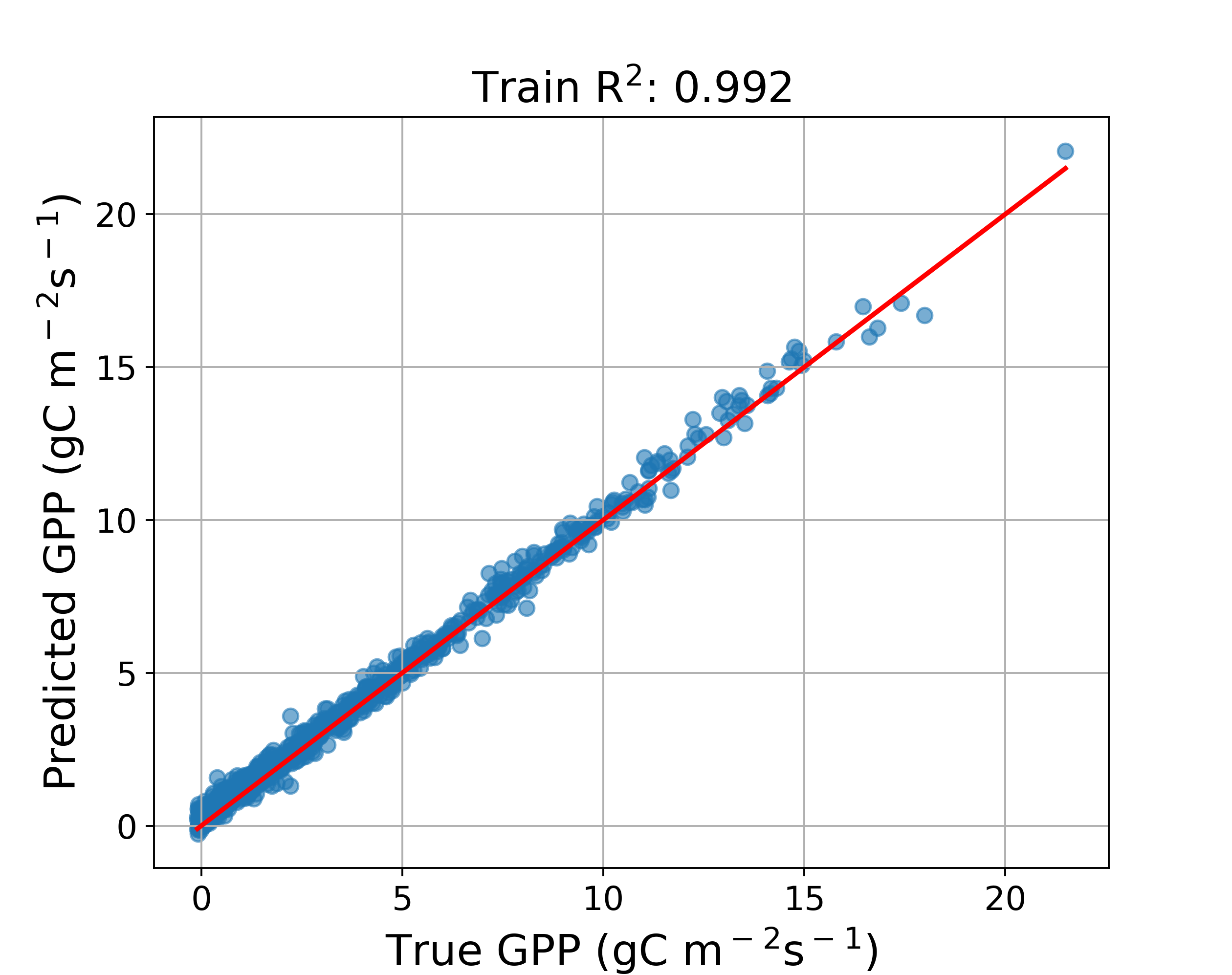
(a) Train: 2019-2021 (889 samples)

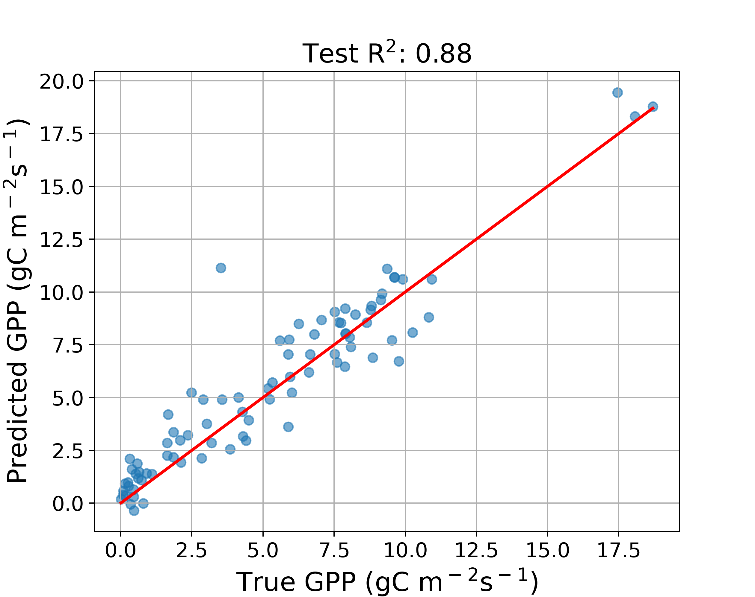
(b) Test: 2018 (86 samples)

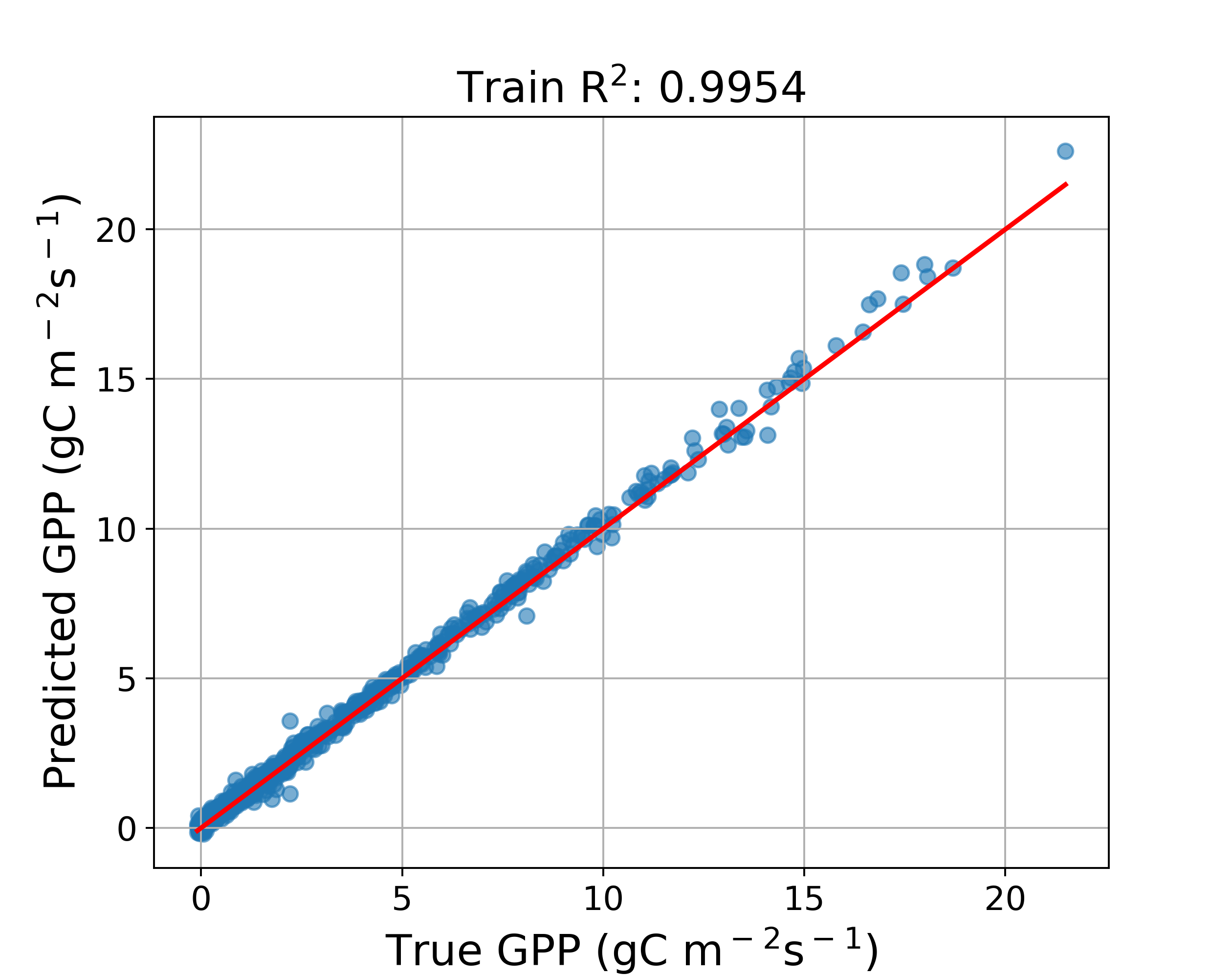
(c) Train: 2018,2020,2021 (693 samples)

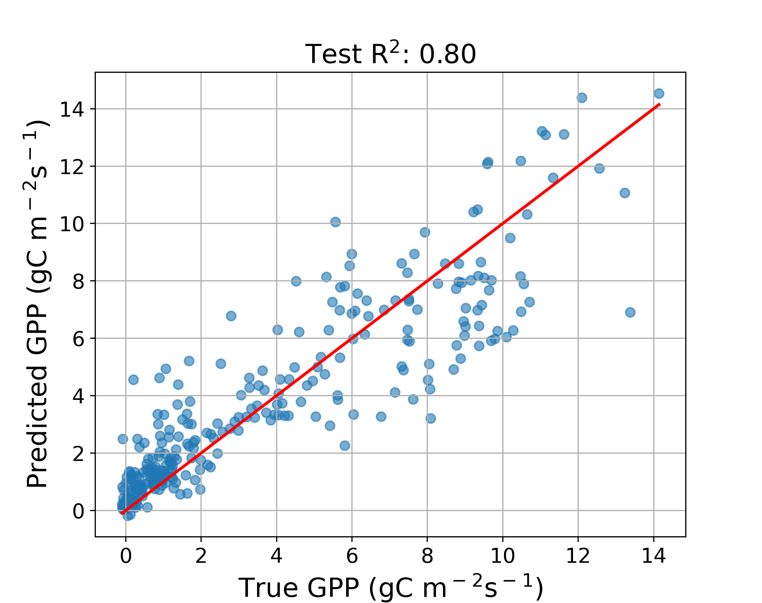
(d) Test: 2019 (282 samples)

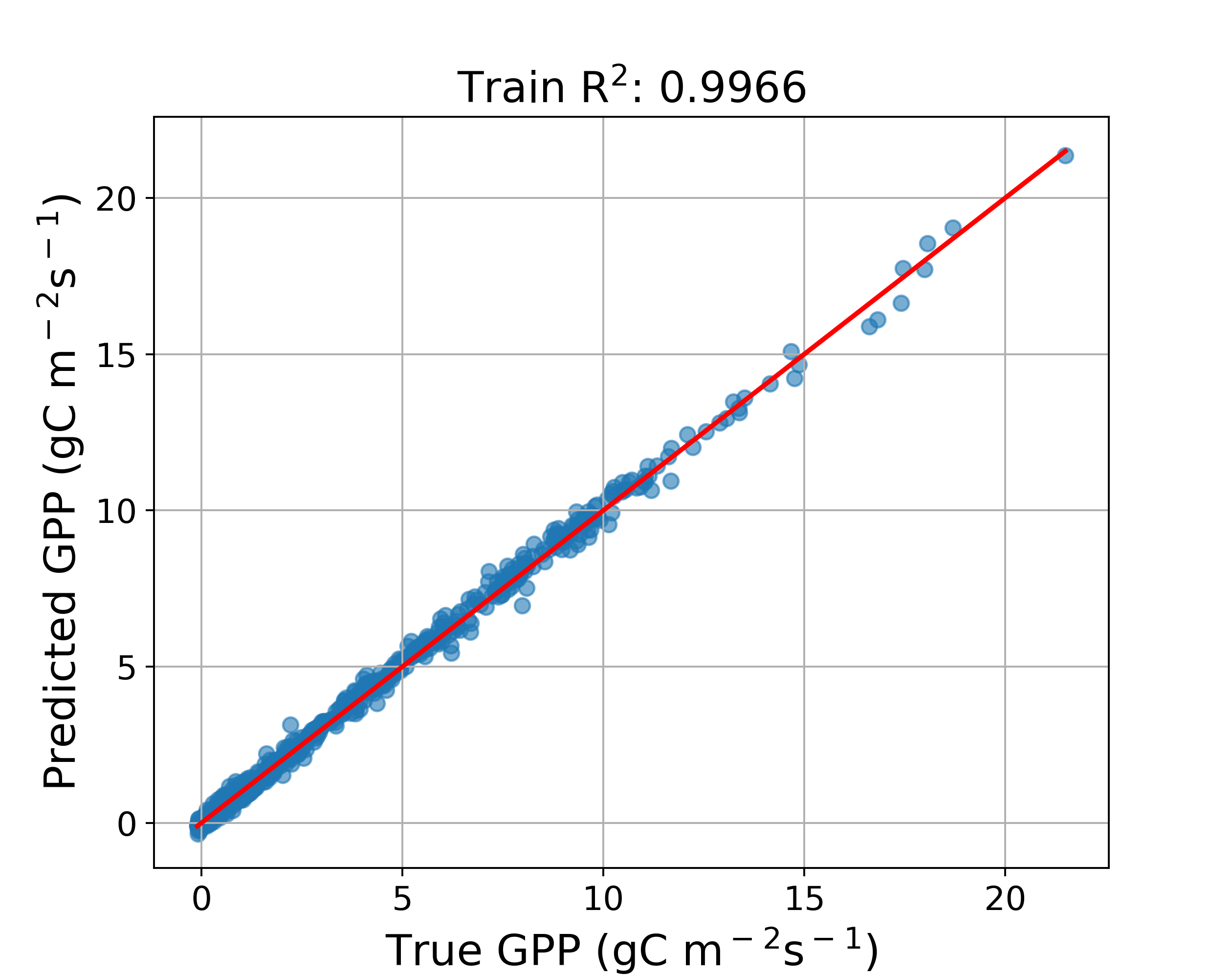
(e) Train: 2018,2019,2021 (688 samples)

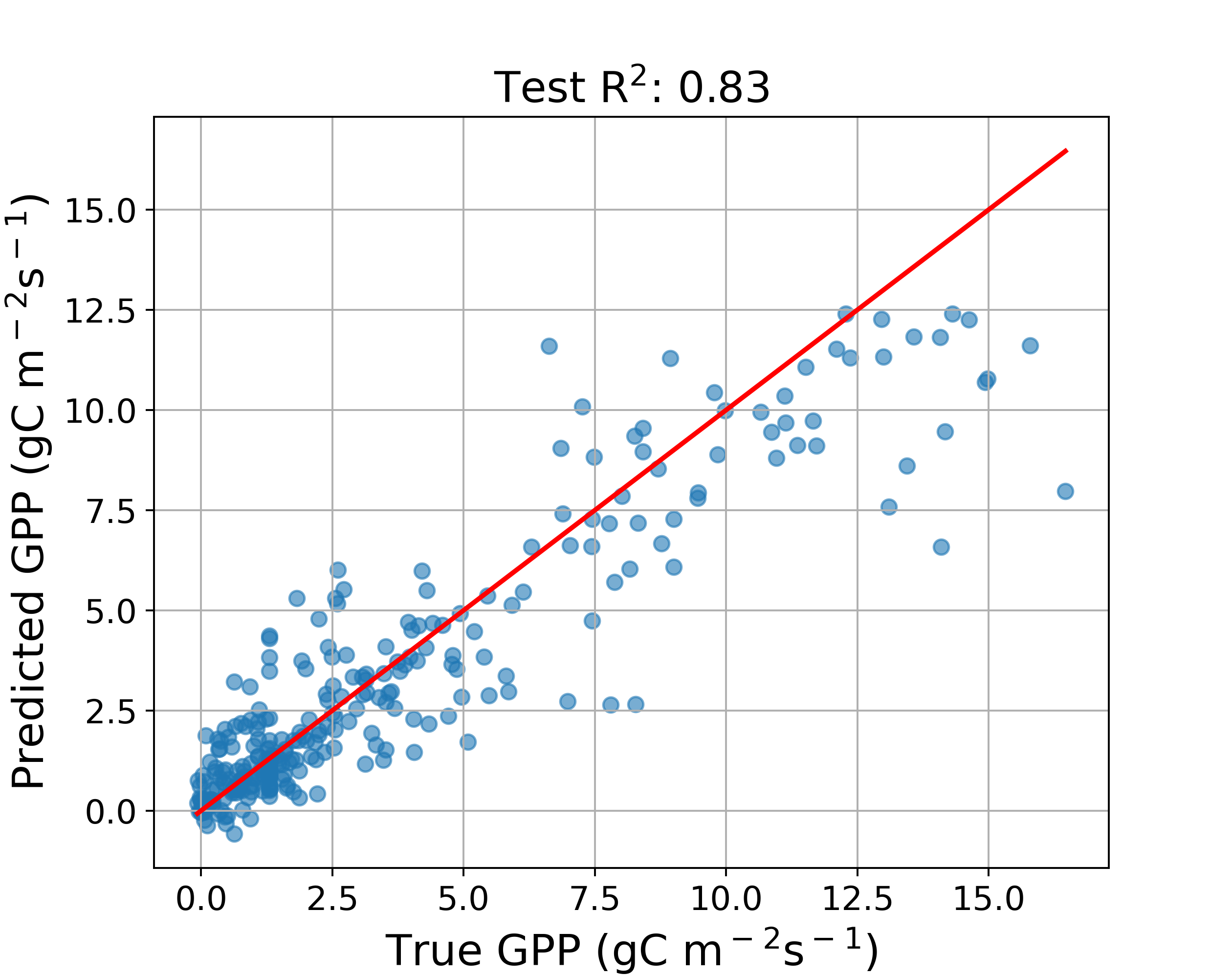
(f) Test: 2020 (287 samples)

(g) Train: 2018-2020 (655 samples)

(h) Test: 2021 (320 samples)

Figure 17: Train test set $R^{2}$ for GPP flux estimation using the leave one year out cross validation over 975 instances of HLS and MERRA-2 data using Prithvi-EO-2.0-600M-TL.

The dataset structure combines three primary components: (1) HLS 6-band reflectance data organized as 50$\times$50$\times$6 pixels (TIFF files), (2) 10-dimensional Modern-Era Retrospective analysis for Research and Applications version 2 (MERRA-2) atmospheric and land surface variables capturing environmental conditions, and (3) daily GPP measurements derived using the night-time partitioning approach. HLS and MERRA-2 data are centered on flux tower locations. The GPP data span 37 globally distributed flux tower sites from 2018 to 2021, encompassing 975 samples. MERRA-2 variables include minimum, maximum, and mean temperatures, soil moisture, heat flux, radiation, precipitation, and other key environmental metrics, identified using specific M2T1NXSLV and M2T1NXLND codes.

The dataset preparation process involves meticulous filtering and quality checks. HLS data are pre-selected based on a 25% maximum cloud threshold and 75% minimum spatial coverage threshold, with further filtering to remove scenes with $>$2% snow cover and $>$5% cloud cover. HLS reflectance values are scaled accordingly. MERRA-2 data are aggregated as daily mean values for each flux site. Instances with GPP values $\leq-0.1gCm^{-2}s^{-1}$, indicative of poor data, are removed. Corresponding HLS and MERRA-2 inputs for each GPP record are matched, and additional filters exclude data with Enhanced Vegetation Index (EVI) values $\leq-0.1$, which signal snow or cloud contamination. EVI values are computed as spatial averages over the HLS chips. This dataset provides a high-quality, integrated framework of remote sensing and ground observations for studying GPP dynamics under diverse environmental conditions.

We adapt the trained Prithvi models to the task of predicting GPP by using the six-band HLS reflectance data and combine the ten input features from MERRA-2 (selected by the subject matter expert), characterizing the atmospheric and land surface properties corresponding to each observation. The fine-tuning architecture designed for this task is shown in Figure 16. To train the models, the multispectral HLS input is passed through the trained and frozen Prithvi encoder to derive encoded HLS representation (Prithvi embeddings) of the flux observation sites, which are then passed through a simple decoder with two linear layers with ReLU activation and flattened. The MERRA-2 input features co-located with flux sites are transformed in parallel via a separate branch consisting of three 2-D convolutional and a linear layer with ReLU activations and then flattened. The flattened HLS representation (from Prithvi encoder and simple decoder) and flattened MERRA-2 representation are then concatenated and regressed to predict the GPP values using a linear layer. The models are trained by minimizing the mean squared error loss between the predicted GPP and true GPP. The approach is designed to facilitate augmenting the Prithvi HLS representation with additional environmental variables and combine multisensor satellite data to predict GPP values at flux tower sites. In the test phase, we pass the HLS data, MERRA-2 data to the model for predicting GPP. Data splitting for training and evaluation follows a leave-one-year-out cross-validation approach, where three years are used for training and one year for testing to mitigate the challenges posed by the relatively small dataset size.

Table 13: $R^{2}$ analysis of baseline model Random Forest vs Prithvi (VIs - vegetation indices, Prithvi Models do not use additional VI) using a leave-one year out cross validation approach over 975 globally distributed flux towers. The years shown here indicate the test set.

Models	2018	2019	2020	2021
RF (-VIs)	0.68	0.78	0.70	0.64
RF (+VI)	0.72	0.77	0.73	0.66
Prithvi-EO-2.0-300M-TL	0.84	0.76	0.74	0.69
Prithvi-EO-2.0-600M-TL	0.88	0.80	0.83	0.74

These steps are replicated with all four variants of Prithvi models and we quantify the model’s skill in predicting GPP using the coefficient of determination, $R^{2}$ measure between the predicted and true GPP values. The $R^{2}$ performance in each train test split across all years is shown in Figure 17. Prithvi is also compared to a baseline model based on random forest, which uses the spatial average of HLS bands across each chip and the MERRA-2 data, representing the state-of-the-art approaches [39]. The baseline model also incorporated vegetation indices, including EVI, Normalized Difference Vegetation Index (NDVI), Normalized Difference Water Index (NDWI), Green Chlorophyll Index (GCI), near-infrared reflectance of vegetation (NIRv), and kernel NDVI. Results in Table 13 show that Prithvi-EO-2.0 models performed better than the random forest without vegetation indexes with up-to 20% improvement on $R^{2}$. Furthermore, the Prithvi-EO-2.0-600M version with temporal and location embeddings consistently outperformed the random forest including the vegetation indexes despite not having this information in its input. The proposed fine-tuning approach using Prithvi-EO-2.0 and MERRA-2 data shows promise for expanding the study to additional flux tower sites and extrapolating GPP beyond the flux network to derive a key climatic variable.

5 Conclusion

We presented Prithvi-EO-2.0, the second iteration of the Prithvi-EO family. Prithvi-EO-2.0 showed strong performance in both standard benchmarking experiments at different resolutions, where it improved up-to 8% its predecessor and outperformed some of the most popular GFMs on GEO-Bench [5]. Prithvi-EO-2.0 also showed state-of-the-art results across a range of SME-led real-world applications in disaster response, land use and crop mapping, and ecosystem dynamics monitoring. Key to the success of this multi-disciplinary cross-institution project was developing a carefully-crafted unbiased multi-temporal dataset for pretraining, and the transparent and thorough evaluation of many aspects of Prithvi-EO-2.0. The project exemplifies the Trusted Open Science Pledge that all project partners subscribed to. In this spirit, we release our models with a permissive license in two different sizes (300M and 600M) on Hugging Face. To maximize community impact and lower entry barriers, we have also onboarded the models in terratorch for easy customization and adoption.

Acknowledgments This work is supported by NASA Grant 80MSFC22M004. We want to express our gratitude to Hugging Face for hosting Prithvi, associated demos, and the corresponding datasets for fine-tuning. The authors gratefully acknowledge the Gauss Centre for Supercomputing e.V. (www.gauss-centre.eu) for funding this project by providing computing time through the John von Neumann Institute for Computing (NIC) on the GCS Supercomputer JUWELS [15] at Jülich Supercomputing Centre (JSC).

References

- \bibcommenthead
- Tuia et al. [2024] Tuia, D., Schindler, K., Demir, B., Zhu, X.X., Kochupillai, M., Džeroski, S., Rijn, J.N., Hoos, H.H., Del Frate, F., Datcu, M., et al.: Artificial intelligence to advance earth observation: A review of models, recent trends, and pathways forward. IEEE Geoscience and Remote Sensing Magazine (2024)
- Tseng et al. [2023] Tseng, G., Cartuyvels, R., Zvonkov, I., Purohit, M., Rolnick, D., Kerner, H.: Lightweight, pre-trained transformers for remote sensing timeseries. arXiv preprint arXiv:2304.14065 (2023)
- Dumeur et al. [2024] Dumeur, I., Valero, S., Inglada, J.: Self-supervised spatio-temporal representation learning of satellite image time series. IEEE Journal of Selected Topics in Applied Earth Observations and Remote Sensing (2024)
- Jakubik et al. [2023] Jakubik, J., et al.: Foundation models for generalist geospatial artificial intelligence. arXiv preprint arXiv:2310.18660 (2023) arXiv:2310.18660 [cs.CV]
- Lacoste et al. [2024] Lacoste, A., Lehmann, N., Rodriguez, P., Sherwin, E., Kerner, H., Lütjens, B., Irvin, J., Dao, D., Alemohammad, H., Drouin, A., et al.: Geo-bench: Toward foundation models for earth monitoring. Advances in Neural Information Processing Systems 36 (2024)
- Claverie et al. [2018] Claverie, M., Ju, J., Masek, J.G., Dungan, J.L., Vermote, E.F., Roger, J.-C., Skakun, S.V., Justice, C.: The Harmonized Landsat and Sentinel-2 Surface Reflectance Data Set. Remote Sensing of Environment 219, 145–161 (2018)
- Buchhorn et al. [2020] Buchhorn, M., Smets, B., Bertels, L., De Roo, B., Lesiv, M., Tsendbazar, N.-E., Herold, M., Fritz, S.: Copernicus global land service: land cover 100 m: collection 3: epoch 2019: Globe. URL: https://zenodo.org/record/3939050 (2020)
- Dinerstein et al. [2017] Dinerstein, E., Olson, D., Joshi, A., Vynne, C., Burgess, N.D., Wikramanayake, E., Hahn, N., Palminteri, S., Hedao, P., Noss, R., et al.: An ecoregion-based approach to protecting half the terrestrial realm. BioScience 67(6), 534–545 (2017)
- He et al. [2022] He, K., Chen, X., Xie, S., Li, Y., Dollár, P., Girshick, R.: Masked Autoencoders Are Scalable Vision Learners. In: Proceedings of the IEEE/CVF Conference on Computer Vision and Pattern Recognition, pp. 16000–16009 (2022)
- Tong et al. [2022] Tong, Z., Song, Y., Wang, J., Wang, L.: Videomae: Masked Autoencoders Are Data-Efficient Learners for Self-Supervised Video Pre-Training. Preprint Available on arXiv:2203.12602 (2022)
- Cong et al. [2022] Cong, Y., Khanna, S., Meng, C., Liu, P., Rozi, E., He, Y., Burke, M., Lobell, D., Ermon, S.: Satmae: Pre-Training Transformers for Temporal and Multi-Spectral Satellite Imagery. Advances in Neural Information Processing Systems 35, 197–211 (2022)
- Reed et al. [2023] Reed, C.J., Gupta, R., Li, S., Brockman, S., Funk, C., Clipp, B., Keutzer, K., Candido, S., Uyttendaele, M., Darrell, T.: Scale-mae: A scale-aware masked autoencoder for multiscale geospatial representation learning. In: Proceedings of the IEEE/CVF International Conference on Computer Vision, pp. 4088–4099 (2023)
- Feichtenhofer et al. [2022] Feichtenhofer, C., fan, h., Li, Y., He, K.: Masked Autoencoders as Spatiotemporal Learners. In: Advances in Neural Information Processing Systems, vol. 35, pp. 35946–35958 (2022)
- Sedona et al. [2019] Sedona, R., Cavallaro, G., Jitsev, J., Strube, A., Riedel, M., Benediktsson, J.: Remote Sensing Big Data Classification with High Performance Distributed Deep Learning. MDPI AG (2019). https://doi.org/10.3390/rs11243056
- Jülich Supercomputing Centre [2021] Jülich Supercomputing Centre: JUWELS Cluster and Booster: Exascale Pathfinder with Modular Supercomputing Architecture at Juelich Supercomputing Centre. Journal of large-scale research facilities 7(A138) (2021) https://doi.org/10.17815/jlsrf-7-183
- Ronneberger et al. [2015] Ronneberger, O., Fischer, P., Brox, T.: U-net: Convolutional networks for biomedical image segmentation. In: Proceedings of the 18th International Conference on Medical Image Computing and Computer-Assisted Intervention (MICCAI), pp. 234–241 (2015)
- Xiao et al. [2018] Xiao, T., Liu, Y., Zhou, B., Jiang, Y., Sun, J.: Unified perceptual parsing for scene understanding. In: Proceedings of the European Conference on Computer Vision (ECCV), pp. 418–434 (2018)
- Wang et al. [2023] Wang, Y., Braham, N.A.A., Xiong, Z., Liu, C., Albrecht, C.M., Zhu, X.X.: Ssl4eo-s12: A large-scale multimodal, multitemporal dataset for self-supervised learning in earth observation [software and data sets]. IEEE Geoscience and Remote Sensing Magazine 11(3), 98–106 (2023)
- Wang et al. [2024] Wang, Y., Albrecht, C.M., Braham, N.A.A., Liu, C., Xiong, Z., Zhu, X.X.: Decoupling common and unique representations for multimodal self-supervised learning. In: 18th European Conference on Computer Vision, ECCV 2024, pp. 1–19 (2024). Springer
- Xiong et al. [2024] Xiong, Z., Wang, Y., Zhang, F., Stewart, A.J., Hanna, J., Borth, D., Papoutsis, I., Le Saux, B., Camps-Valls, G., Zhu, X.X.: Neural plasticity-inspired foundation model for observing the earth crossing modalities. arXiv e-prints, 2403 (2024)
- Bastani et al. [2023] Bastani, F., Wolters, P., Gupta, R., Ferdinando, J., Kembhavi, A.: Satlaspretrain: A large-scale dataset for remote sensing image understanding. In: Proceedings of the IEEE/CVF International Conference on Computer Vision, pp. 16772–16782 (2023)
- Büttner [2014] Büttner, G.: CORINE Land Cover and Land Cover Change Products. Springer (2014). https://doi.org/10.1007/978-94-007-7969-3_5 . http://dx.doi.org/10.1007/978-94-007-7969-3_5
- Bonafilia et al. [2020] Bonafilia, D., Tellman, B., Anderson, T., Issenberg, E.: Sen1Floods11: A Georeferenced Dataset to Train and Test Deep Learning Flood Algorithms for Sentinel-1. In: Proceedings of the IEEE/CVF Conference on Computer Vision and Pattern Recognition Workshops, pp. 210–211 (2020)
- Napper [2006] Napper, C.: Burned Area Emergency Response Treatments Catalog. US Forest Service, San Dimas Technology and Development Center, ??? (2006)
- Ghorbanzadeh et al. [2022] Ghorbanzadeh, O., Xu, Y., Zhao, H., Wang, J., Zhong, Y., Zhao, D., Zang, Q., Wang, S., Zhang, F., Shi, Y., Zhu, X.X., Bai, L., Li, W., Peng, W., Ghamisi, P.: The outcome of the 2022 landslide4sense competition: Advanced landslide detection from multisource satellite imagery. IEEE Journal of Selected Topics in Applied Earth Observations and Remote Sensing 15, 9927–9942 (2022) https://doi.org/10.1109/JSTARS.2022.3220845
- Berman et al. [2018] Berman, M., Triki, A.R., Blaschko, M.B.: The lovász-softmax loss: A tractable surrogate for the optimization of the intersection-over-union measure in neural networks. In: Proceedings of the IEEE Conference on Computer Vision and Pattern Recognition, pp. 4413–4421 (2018)
- Loshchilov and Hutter [2016] Loshchilov, I., Hutter, F.: Sgdr: Stochastic gradient descent with warm restarts. arXiv preprint arXiv:1608.03983 (2016)
- Ronneberger et al. [2015] Ronneberger, O., Fischer, P., Brox, T.: "U-Net: Convolutional Networks for Biomedical Image Segmentation". In: Proceedings of the 18th International Conference on Medical Image Computing and Computer-Assisted Intervention (MICCAI), pp. 234–241 (2015)
- Zhou et al. [2018] Zhou, Z., Rahman Siddiquee, M.M., Tajbakhsh, N., Liang, J.: Unet++: A nested u-net architecture for medical image segmentation. In: Deep Learning in Medical Image Analysis and Multimodal Learning for Clinical Decision Support: 4th International Workshop, DLMIA 2018, and 8th International Workshop, ML-CDS 2018, Held in Conjunction with MICCAI 2018, Granada, Spain, September 20, 2018, Proceedings 4, pp. 3–11 (2018). Springer
- Li et al. [2023] Li, W., Lee, H., Wang, S., Hsu, C.-Y., Arundel, S.T.: Assessment of IBM and NASA’s Geospatial Foundation Model in Flood Inundation Mapping. Preprint Available on arXiv:2309.14500 (2023)
- Ghorbanzadeh et al. [2022] Ghorbanzadeh, O., Xu, Y., Zhao, H., Wang, J., Zhong, Y., Zhao, D., Zang, Q., Wang, S., Zhang, F., Shi, Y., et al.: The outcome of the 2022 landslide4sense competition: Advanced landslide detection from multisource satellite imagery. IEEE Journal of Selected Topics in Applied Earth Observations and Remote Sensing 15, 9927–9942 (2022)
- Ling et al. [2024] Ling, Y., Wang, Y., Lin, Y., Chan, T.O., Awange, J.: Optimized landslide segmentation from satellite imagery based on multi-resolution fusion and attention mechanism. IEEE Geoscience and Remote Sensing Letters (2024)
- Sharma et al. [2024] Sharma, S., Sedona, R., Riedel, M., Cavallaro, G., Paris, C.: Sen4map: Advancing mapping with sentinel-2 by providing detailed semantic descriptions and customizable land-use and land-cover data. IEEE Journal of Selected Topics in Applied Earth Observations and Remote Sensing 17, 13893–13907 (2024) https://doi.org/10.1109/JSTARS.2024.3435081
- d’Andrimont et al. [2020] d’Andrimont, R., Yordanov, M., Martinez-Sanchez, L., Eiselt, B., Palmieri, A., Dominici, P., Gallego, J., Reuter, H.I., Joebges, C., Lemoine, G., Velde, M.: Harmonised lucas in-situ land cover and use database for field surveys from 2006 to 2018 in the european union. Scientific Data 7(1) (2020) https://doi.org/10.1038/s41597-020-00675-z
- Garnot and Landrieu [2021] Garnot, V.S.F., Landrieu, L.: Panoptic Segmentation of Satellite Image Time Series With Convolutional Temporal Attention Networks. In: Proceedings of the IEEE/CVF International Conference on Computer Vision, pp. 4872–4881 (2021)
- Keenan et al. [2023] Keenan, T.F., Luo, X., Stocker, B.D., De Kauwe, M.G., Medlyn, B.E., Prentice, I.C., Smith, N., Terrer, C., Wang, H., Zhang, Y., et al.: A constraint on historic growth in global photosynthesis due to rising co2. Nature Climate Change 13(12), 1376–1381 (2023)
- Baldocchi [2020] Baldocchi, D.D.: How eddy covariance flux measurements have contributed to our understanding of global change biology. Global change biology 26(1), 242–260 (2020)
- Jung et al. [2020] Jung, M., Schwalm, C., Migliavacca, M., Walther, S., Camps-Valls, G., Koirala, S., Anthoni, P., Besnard, S., Bodesheim, P., Carvalhais, N., et al.: Scaling carbon fluxes from eddy covariance sites to globe: synthesis and evaluation of the fluxcom approach. Biogeosciences 17(5), 1343–1365 (2020)
- Kang et al. [2023] Kang, Y., Gaber, M., Bassiouni, M., Lu, X., Keenan, T.: Cedar-gpp: spatiotemporally upscaled estimates of gross primary productivity incorporating co 2 fertilization. Earth System Science Data Discussions 2023, 1–51 (2023)
- Pastorello et al. [2020] Pastorello, G., Trotta, C., Canfora, E., Chu, H., Christianson, D., Cheah, Y.-W., Poindexter, C., Chen, J., Elbashandy, A., Humphrey, M., et al.: The fluxnet2015 dataset and the oneflux processing pipeline for eddy covariance data. Scientific data 7(1), 225 (2020)
- Team [2022] Team, W.W..: Warm Winter 2020 ecosystem eddy covariance flux product for 73 stations in FLUXNET—release 2022-1 (Version 1.0). ICOS Carbon Portal. https://doi.org/10.18160/2G60-ZHAK (2022)