Resource-Adaptive Successive Doubling for Hyperparameter Optimization with Large Datasets on High-Performance Computing Systems

Abstract

The accuracy of Machine Learning (ML) models is highly dependent on the hyperparameters that have to be chosen by the user before the training. However, finding the optimal set of hyperparameters is a complex process, as many different parameter combinations need to be evaluated, and obtaining the accuracy of each combination usually requires a full training run. It is therefore of great interest to reduce the computational runtime of this process. On High-Performance Computing (HPC) systems, several configurations can be evaluated in parallel to speed up this Hyperparameter Optimization (HPO). State-of-the-art HPO methods follow a bandit-based approach and build on top of successive halving, where the final performance of a combination is estimated based on a lower than fully trained fidelity performance metric and more promising combinations are assigned more resources over time. Frequently, the number of epochs is treated as a resource, letting more promising combinations train longer. Another option is to use the number of workers as a resource and directly allocate more workers to more promising configurations via data-parallel training. This article proposes a novel Resource-Adaptive Successive Doubling Algorithm (RASDA), which combines a resource-adaptive successive doubling scheme with the plain Asynchronous Successive Halving Algorithm (ASHA). Scalability of this approach is shown on up to 1,024 Graphics Processing Units on modern HPC systems. It is applied to different types of Neural Networks and trained on large datasets from the Computer Vision (CV), Computational Fluid Dynamics (CFD), and Additive Manufacturing (AM) domains, where performing more than one full training run is usually infeasible. Empirical results show that RASDA outperforms ASHA by a factor of up to $1.9$ with respect to the runtime. At the same time, the solution quality of final ASHA models is maintained or even surpassed by the implicit batch size scheduling of RASDA. With RASDA, systematic HPO is applied to a terabyte-scale scientific dataset for the first time in the literature, enabling efficient optimization of complex models on massive scientific data.

1 Introduction

In recent years, the amount of openly available data has drastically increased. This includes datasets from different scientific fields, such as CV [43], Earth Observation (EO) [45], High-Energy Physics (HEP) [41], AM [9], or CFD [4]. To analyze these data efficiently and gain novel insights based on hidden correlations, the use of Deep Learning (DL) techniques and NNs has become essential due to their ability to automatically extract complex patterns. As the prediction quality of these NN models is highly dependent on the so-called hyperparameters, which are frequently related to, e.g., the NN architecture or the optimizer, systematic HPO has become a crucial ingredient of ML workflows [12]. However, this search for optimal combinations of hyperparameters is challenging due to often high-dimensional search spaces. Furthermore, the performance of a sample from the search space can only be evaluated with a high degree of confidence after a full model training run. In the case of deep NNs trained on large datasets, this can become a major hurdle, even with extensive computing resources. Additionally, the search space is often diverse in nature. For example, the search space could be comprised of the learning rate, an optimizer-related parameter represented as floating point number, and the number of layers, an architectural parameter represented as an integer number $l>0$. Categorical values, such as “type of optimizer” or “type of layer” are also possible. This makes the application of classical, gradient-based optimization methods infeasible. Hyperparameters also change under different models and datasets, making the generalization difficult to assess. One of the state-of-the-art HPO methods is the ASHA [30]. It randomly samples multiple combinations, evaluates their performance with a lower training budget and then – after comparing their performance – terminates under-performing trials early on. To reduce the time to solution, ASHA is frequently executed in parallel, where multiple NN configurations (trials) are evaluated at the same time.

Modern HPC systems offer a natural setting for running this kind of workload. They feature accelerators, such as GPUs, that are ideally suited for efficient NN trainings (fast computation). Furthermore, these accelerators are connected by an optimized communication network that enables fast inter-node communication. While current distributed HPO methods, such as ASHA, leverage the fast computation capabilities to train different hyperparameter candidates, the communication requirements are usually modest and limited to the exchange of the value of a certain metric, e.g., the current loss on the validation set for the comparison of the performance between trials.

This work introduces a novel method, the RASDA, that leverages both HPC features to perform HPO efficiently at scale. It combines two levels of parallelism: (i) on the HPO level, different trials are run in parallel and (ii) on the level of each trial run, the NN training is accelerated with data-parallel training. The latter splits the datasets onto multiple GPUs and performs gradient synchronization after each training step. As these gradients are typically large, they require high-bandwidth communication. RASDA then leverages the successive doubling principle, which progressively allocates more resources to more promising hyperparameter combinations, treating the amount of GPUs that are used for data-parallel training as resources (performing a doubling in space). In contrast, other successive halving techniques, such as the plain ASHA, treat the number of epochs during training of a model as resources and thus perform only halving in time, see Fig. 1.

The developed method is suitable for problems that involve large scientific datasets, where due to long training times, even with HPC resources it is not feasible to train more than the initially sampled hyperparameter configurations and users are interested in getting the best possible, fully-trained model in the shortest amount of time. Therefore, this study performs an extensive evaluation of RASDA on different datasets from the CV, CFD, and AM domains, which are up to 8.3  Terrabyte (TB) in size, to prove its capability to deal with large datasets. These datasets are used to tune the hyperparameters of different types of NNs, namely a Convolutional Neural Network (CNN), an autoencoder and a transformer. RASDA is also benchmarked against the current state-of-the-art successive halving HPO method ASHA. The new RASDA code is openly available on GitHub for the community.

This article is structured as follows. Section 2 summarizes the related work and highlights the differences to this work. The main details of RASDA are presented in Sec. 3. The application cases are explained in Sec. 4, followed by a presentation and discussion of the empirical results of the algorithm in Sec. 5. Finally, a summary and outlook are provided in Sec. 6.

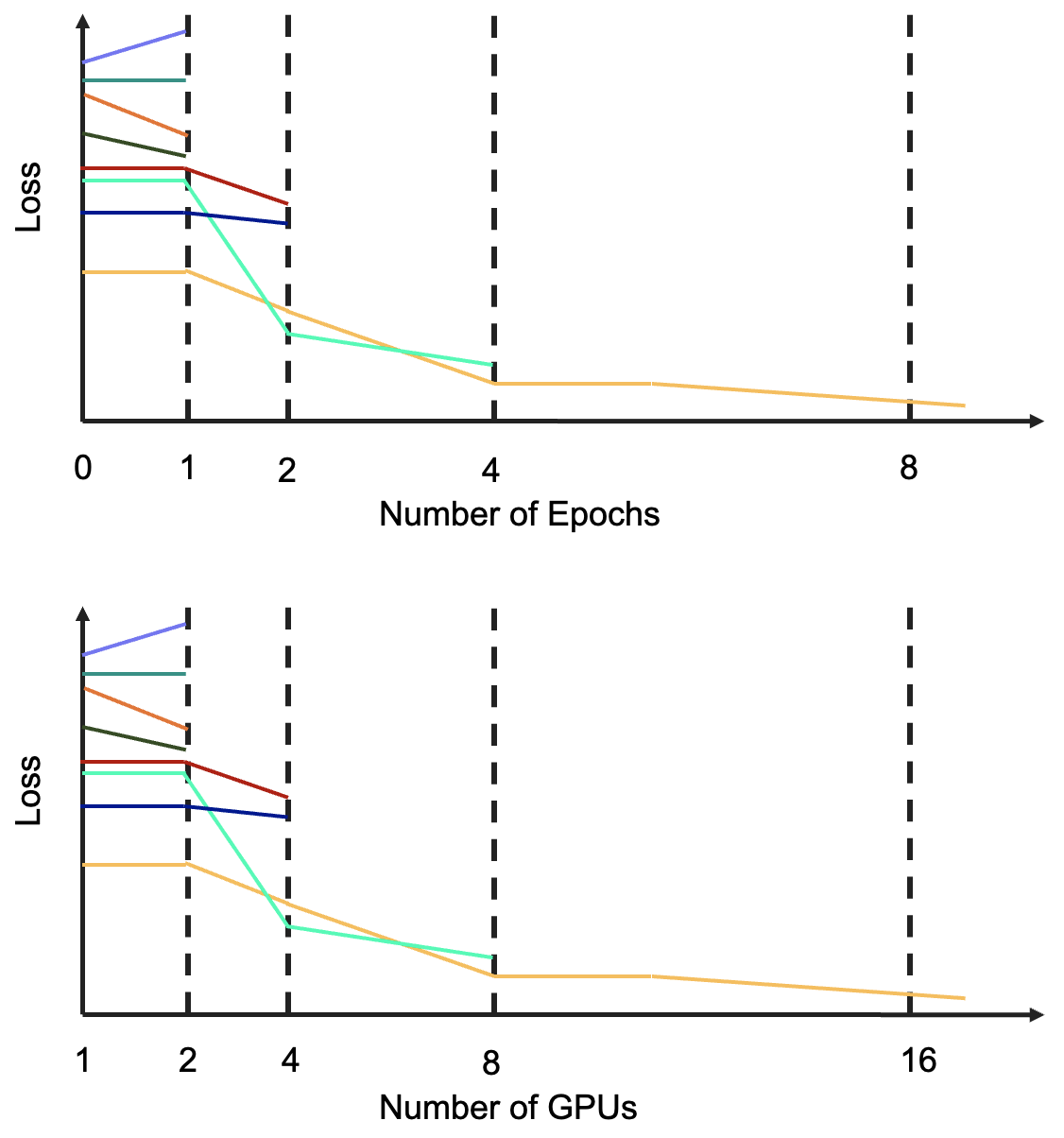
Figure 1: Comparison of successive halving in time (top) and halving in time combined with doubling in space (bottom). Each line corresponds to the learning curve of a single HPO combination.

2 Related Work

In ML, the performance of a certain model measured by a specific metric, such as the validation error, can be represented by the function $f:\mathcal{X}\rightarrow\mathbb{R}$ where $\mathcal{X}$ denotes the space of possible hyperparameter combinations. The primary goal of HPO is to minimize the objective function $f$ by identifying a hyperparameter configuration $x^{*}\in\mathcal{X}$ such that $x^{*}\in\arg\min_{x\in\mathcal{X}}f(x)$. Evaluations of the objective function are costly because they typically involve fully training the model for each configuration. To optimize this workflow, several approaches exist. These are either based on approximating $f(x)$ by a lower fidelity estimate, e.g., by the performance after a few training epochs or a model trained on a fraction of the data, or on choosing better hyperparameter configurations to evaluate, e.g., using Bayesian optimization (BO)). This section summarizes these approaches, i.e. Sec. 2.1 describes the successive halving method, Sec. 2.2 and Sec. 2.3 summarize resource-adaptive as well as other HPO algorithms and Sec. 2.4 introduces the concept of data-parallel training.

2.1 Successive Halving

Successive halving is a variant of Random Search [8], which uses the fact that most ML algorithms are iterative in nature. Intermediate performance results are thus accessible long before the algorithm is fully trained. The problem of finding optimal hyperparameters in a vast search space can then be framed in the context of a multi-armed bandit problem, where each arm represents a hyperparameter combination, and pulling an arm corresponds to training the combination for some iterations [21]. The goal is to identify the arm that yields the highest reward with the lowest budget possible. To do so in an efficient way, successive halving uniformly allocates an initial budget $B$ to $n_{arms}$ arms and evaluates their performance after a few iterations at a milestone with budget $B/n_{arms}$. It then eliminates the worst-performing half of the arms and promotes the most promising-performing arms by continuing to pull them. Each of these successive halving steps is referred to as a rung. When following this procedure for a few steps from rung to rung, only one arm, i.e., the one with the best performance, remains at the end. Hyperband (HB) [29] extends this concept by iterating over different numbers of initial arms $n_{arms}$ (also referred to as brackets) to evaluate.

However, when performing HPO at a larger scale, these methods are sensitive to so-called stragglers. To determine the combinations belonging to the under- and top-performing half, the performance measurement for all combinations needs to be available, which means that faster trials need to wait for the slower ones. ASHA addresses this scalability problem by deciding on a rolling basis which trials are worth continuing. When two trials have finished their initial number of iterations, the trial with the better performance is promoted. At the same time, the other trial is paused until the performance of the next completed trial can be juxtaposed. In contrast to HB, ASHA is mostly performed with only a single bracket, and was evaluated on up to $500$ GPUs in [30].

Another possibility of finding a minimum of the objective function $f$ is to use black-box optimization methods such as BO. The idea behind BO is to use a probabilistic model of $f$ that is based on data points observed in the past. In the case of HPO, this corresponds to finding new promising hyperparameter combinations based on the performance of past combinations. The Bayesian Optimization and HyperBand (BOHB) algorithm [11] combines the BO process with HB for scheduling. To this aim, HB is used to choose the number of hyperparameter configurations and their assigned budget, while BO is used to choose the hyperparameters by deploying a tree parzen estimator [7].

The mentioned methods have in common that they focus only on identifying the most promising arm and delivering that hyperparameter combination as a result at the end of a run. In contrast, RASDA also ensures the full training of the best combination to yield a complete model.

2.2 Resource-Adaptive Schedulers

Most of the existing successive halving-based HPO schedulers treat the number of epochs or training time as resources (also known as fidelity in the literature). It is, however, also possible to treat the spatial amount of computational resources, e.g., the number of GPU, used for training a model as a fidelity. A low-fidelity measurement then corresponds to the performance of a NN trained with a small number of devices. The most relevant existing HPO schedulers that focus on this computational resource-adaptive scheduling are presented in the following.

HyperSched [32] introduces a scheduler to dynamically allocate resources in time and space to the best-performing hyperparameter trials. It thereby not only identifies the most promising model but also trains it – ideally fully – by a fixed deadline. The main novelty of the algorithm is its deadline awareness, which means that it schedules fewer new trials as it approaches the deadline. This way, the exploration of new configurations is stopped in favor of deeper exploitation of the running trials. HyperSched is evaluated in [32] on different CV benchmarking datasets on up to 32 GPUs on Cloud computing instances.

Rubberband [40] extends HyperSched by leveraging the elasticity of the Cloud for the task of scheduling HPO workloads. It takes into account not only the performance of a combination but also the financial costs of a GPU hour, with the goal of minimizing the costs of an HPO job. Based on the idea of diminishing returns when scaling the training of a single model, the algorithm de-allocates resources (and thus saves costs) from less-promising trials, once a promising trial has been identified. It also creates a resource allocation plan a priori the run to optimize the performance of the single trials that are trained via distributed DL. The resource allocation plan is initialized with an initial burn-in period during which training latencies and scaling performance of trials are measured.

Sequential Elimination with Elastic Resources (SEER) [10] further takes advantage of the elasticity in the cloud by adaptively allocating and de-allocating compute resources during the HPO run. At the same time, it focuses on maximizing the accuracy of trials, in combination with minimizing the total financial cost. Therefore, it limits the amount of workers allocated to the top trials once sub-linear scaling performance sets in.

Both Rubberband and SEER rely heavily on the adaptive allocation and de-allocation of GPU instances, which is possible in an elastic cloud setting but not on HPC systems, where the amount of GPUs allocated to the overall HPO job is usually static. HyperSched, meanwhile, focuses on maximizing the performance by the deadline. In contrast, the proposed RASDA method aims to deliver the best-possible result in the shortest amount of time.

2.3 Other HPO Algorithms and Libraries

Many other algorithms and libraries for performing HPO exist. These include BO-based libraries such as Dragonfly [25] and SMAC [34], allowing the user to select different surrogate models and acquisition functions. Optuna [3] also relies on BO and provides automated tracking and visualization of trials. Since parallel computing resources have become increasingly available in recent years, several algorithms have emphasized large-scale, distributed HPO: DeepHyper [6] focuses on performing asynchronous BO on HPC systems and has been applied to several scientific use cases [5, 22, 35]. Distributed evolutionary optimization can be performed with Propulate [46] and Population Based Training (PBT) [20].

While most of these libraries support multi-fidelity HPO, none of them so far supports performing resource-adaptive scheduling of trials, which is, however, supported by RASDA.

2.4 Data-Parallel Deep Learning

Data-parallel training is a technique to reduce the runtime of the training of DL models on large datasets by using multiple devices, such as GPUs. In data-parallel training, the training dataset $\mathcal{D}$ is divided among the number of workers $N$, where each worker is assigned an identical copy of the model to train on a distinct subset of the data $\mathcal{D}_{1}\cup\mathcal{D}_{2}\cup\ldots\cup\mathcal{D}_{N}$. Specifically, each worker $i=1\dots N$ runs one model forward and backward pass with a predefined number of samples, the local batch size $BS_{local}$, of its subset of data to compute its local gradients $\Delta w_{i}$ with respect to the model parameters $w$. After the backward pass, these local gradients are aggregated and averaged across all workers by

$$\Delta w=\frac{1}{N}\sum_{i=1}^{N}\Delta w_{i},$$ (1)

The averaged global gradient is then used to update the model parameters on all workers every $BS_{global}=BS_{local}\cdot N$ samples [31]. To remain computationally efficient, each worker needs a sufficient amount of data to run the training, thus $BS_{local}$ needs to be large. At the same time, $BS_{global}$ increases linearly with $N$. When $BS_{global}$ becomes too large, it can impact the generalization performance for two reasons. First, the number of optimizer updates per epoch decreases, as an update is performed every $BS_{global}$ samples. This can be addressed to some extent by scaling the learning rate with the number of devices [14]. This approach is, however, infeasible for an extremely large $BS_{global}$, since in such a case also the learning rate becomes too large. Second, Stochastic Gradient Descent (SGD) with large batch sizes tends to converge to sharp minima [17] which does not generalize well, see [26] for more details.

3 Resource-Adaptive Successive Doubling Algorithm

This section presents details on RASDA in Sec. 3.1 and provides an explanation on how issues with large batch size training, cf. Sec. 2.4, are addressed in Sec. 3.2.

(a) ASHA

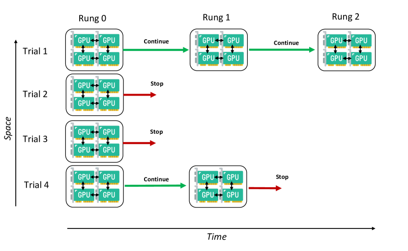
(b) RASDA

Figure 2: Comparison of (plain) ASHA, performing successive halving only in the time domain, and RASDA, performing successive halving in the time and successive doubling in the space domain at the same time on an GPU cluster. In the RASDA case, when a trial is terminated, its workers are allocated to the more promising trials to increase the parallelism of the data-parallel training. Black arrows indicate communication of gradients between GPUs.

Algorithm 1 Resource Adaptive Successive Doubling Method

1:trial_result, base_resources, sf, milestones

2:if trial_result["training_iteration"] $\in$ milestones then

3:     current_rung $\leftarrow$ milestones.index(trial_result["training_iteration"])

4:     new_resources $\leftarrow$ base_resources $\times$ sf${}^{\texttt{current\_rung}}$

5:     return new_resources

6:else

7:     return None

8:end if

3.1 Algorithm Design and Implementation

The main idea of RASDA is to combine a successive halving step in the time domain, i.e., train more promising configurations for longer, and a successive doubling step in the spatial domain, i.e., allocate more workers to more promising configurations. This way, when reaching a rung milestone, the worst-performing trials are terminated (halving in time) and the free workers are allocated to the top-performing trials (doubling in space), see Fig. 2. The additional workers are then used to increase the parallelism of the data-parallel training of the configuration, which leads to faster training times.

For the re-allocation of workers, a second successive doubling routine in addition to the successive halving routine of ASHA is used (the resource allocation part is described in Alg. 1): All trials start out with an initial number of workers
($\mathtt{base\_resources}$). When a trial reports a new $\mathtt{trial\_result}$, it is first checked if the current $\mathtt{training\_}$$\mathtt{iteration}$, e.g., the current epoch, corresponds to one of the rung $\mathtt{mile}$$\mathtt{stones}$. At every rung $\mathtt{milestone}$, the (plain) ASHA scheduler then reduces the number of running trials by the reduction factor $\mathtt{rf}$. The resources for all trials that are allowed to continue are then increased with the scaling factor $\mathtt{sf}$ by the RASDA scheduler, yielding the $\mathtt{new\_resources}$ for the trial (following Alg. 1). If the reduction and scaling factors are equal, i.e. $\mathtt{rf}=\mathtt{sf}$, all workers are continuously allocated to a trial. In practice, however, some trials do run faster than others. The advantage of the ASHA and RASDA scheduler is that they both perform asynchronous halving and doubling, i.e., top-performing trials are promoted to the next rung even if not all trials in the current rung have reached their milestones. This reduces idling times between halving steps. It should be noted that due to this asynchronous execution, the percentage of trials terminated at each milestone can be smaller than $\mathtt{rf}$. As the total number of workers in the system is a constant, the trials that are allowed to continue might need to wait until their new resource requirements are met.

At these rung $\mathtt{milestones}$, two processes occur: the (plain) ASHA scheduler reduces the number of running trials by the reduction factor $\mathtt{rf}$, while Alg.1 handles the reallocation of GPU resources among the remaining trials.

The total number of rungs and their corresponding milestones in the RASDA scheduler are calculated based on the minimum and maximum iterations $\min\_t$ and $\max\_t$, along with the scaling factor $\mathtt{sf}$, as

$$\mathtt{num\_rungs} =\left\lfloor\frac{\log\left(\frac{\max\_t}{\min\_t}\right)}{\log(\mathtt{sf})}\right\rfloor,$$ (2)

$$\mathtt{rung\_milestones} =\min\_t\cdot\mathtt{sf}^{k},$$ (3)

with $k=0,\ldots,\mathtt{num\_rungs}$. This ensures a geometric progression of the milestones, as described for ASHA by Li et al. [30].

The algorithm is implemented with Ray Tune [33], an open-source library for performing distributed HPO. Ray Tune orchestrates the optimization process by launching a single head node and several worker nodes on an HPC cluster. The head node then connects to the worker nodes and starts the trials. During training, the worker nodes report their current status including performance metrics to the head node that makes scheduling decisions, such as termination or continuation of new trials.

Ray Tune already features implementations of several successive halving methods. The implementation of RASDA therefore relies on the implementation of ASHA that exists already inside of Ray Tune for performing the time-wise successive halving. For the spatial successive doubling, RASDA makes use of the ResourceChangingScheduler interface, enabling the modification of resource requirements for trials. At each milestone, the trial is saved, including the current weights of the model. If the decision is made to continue the training, the trial is relaunched with the new resource requirements. It should be noted, that the ASHA implementation of Ray Tune has some minor differences to the original algorithm in [30]. However, empirical evidence shows that these differences do not impact performance.

The data-parallel training part is handled by the PyTorch-DDP library [31], which uses the NVIDIA Collective Communications Library (NCCL) backend for communication and gradient synchronization.

3.2 Large Batch Training

Recall from Sec. 2.4 that scaling the data-parallel training to a large number of devices and increasing $BS_{global}$ can impact the generalization performance of models. The following provides an intuitive explanation of how this issue is addressed by the RASDA scheduler.

McCandlish et al. [39] empirically studied large batch training for various models: they introduce the Gradient Noise Scale (GNS) metric, which serves as a noise-to-signal measure of the training progress. In theory, if the true gradient $G_{true}$ from performing full-batch Gradient Descent without the stochastic component would be available, it would be possible to compute the a simple version of the GNS by

$$\mathrm{GNS}_{simple}=\frac{\mathrm{tr}(\Sigma)}{|G_{true}|^{2}},$$ (4)

where $\Sigma$ is the per-data-sample covariance matrix of $G_{true}$. Essentially, the nominator measures the noise of the gradient, while the denominator measures its magnitude. As the DL model converges, the gradient decreases in size, which results in an increase of the GNS over training time. McCandlish et al. use an approximation to compute the GNS based on the estimated stochastic gradient $G_{est}$ and confirm that the GNS indeed increases over time.

Based on the GNS, Qiao et al. [42] introduce the concept of “statistical efficiency” of the DL training, measuring the amount of training progress made per data sample processed in a batch. The key insight is that when the GNS is low, there is no benefit for the learning progress in adding more data samples to the batch (thus increasing $BS_{global}$), as the stochastic gradient $G_{est}$ is a precise approximation of $G_{true}$ already. However, when the GNS is high, adding more data samples to the batch reduces the noise and leads to a better gradient approximation. As the GNS starts out small and increases over time, this justifies the usage of larger batch sizes during the later part of training. This approach has also been used successfully for HPO and scheduling tasks in the past [42, 2].

Additionally, Smith et al. [44] find that increasing $BS_{global}$ over time has a similar effect as decaying in the learning rate, which is common practice in DL nowadays [36]. Based on these findings, the following two insights can be derived:

• Training with a small $BS_{global}$ generally helps generalization and is computationally efficient at the beginning of training, in terms of the training progress per processed data sample.

• Increasing $BS_{global}$ over time and using a large $BS_{global}$ as the model is converging is computationally efficient as well.

This aligns well with the scheduling of the RASDA algorithm. In the beginning, the trials train with a small $BS_{global}$, i.e., the number of workers allocated for the data-parallel training is small. As time progresses, $BS_{global}$ increases with each resource doubling step, as more and more workers are allocated to the data-parallel training. The evaluation in Sec. 5 shows that by leveraging this approach, the generalization capabilities of the final models match or exceed those of models that are continuously trained with a small $BS_{global}$.

Another crucial point is the correct scaling of the learning rate with the batch size. In the evaluation in Sec. 5, the learning rate is scaled linearly with the number of workers, i.e., up to a factor of $8\times$, when using SGD [28]. Furthermore, it follows a square-root scaling rule when using Adaptive Moment Estimation (ADAM) [37]. In the case of re-scaling, the learning rate is not immediately scaled to a larger value. Instead, there is a warm-up over one or two epochs. This re-scaling parameter is included as a hyperparameter in the search space, see Tab. 1. Thereby, the HPO run automatically optimizes towards learning stability.

3.3 Performance Optimization

To ensure efficient performance, several additional optimizations are made to the trials in the HPO loop. This includes selecting the $BS_{local}$ sufficiently large such that it fills the GPU memory in addition to the model for each of the applications. As the training datasets have to be loaded by each trial in parallel when performing HPO, they are loaded into shared memory when they fit in size. Training datasets that do not fit into shared memory are stored on a partition of the file system with high bandwidth to avoid bottlenecks. For data loading, the native PyTorch data loader as well as the NVIDIA DALI library are used.

A preliminary study determined that saving the model weights into a checkpoint too often can lead to bottlenecks [1]. Therefore, the checkpoint frequency is reduced to every five epochs and the rung milestones of the ASHA and RASDA scheduler are adjusted accordingly. Ray Tune needs an initial start-up time to launch the head node and all connected worker nodes. As this is the same for ASHA and RASDA, these timings are excluded from the measurements.

4 Application Cases

To assess the proposed RASDA scheduler, its performance is evaluated across a range of different tasks from the CV, CFD, and AM domain. These cases feature various models with different hyperparameters to optimize as well as training datasets of different sizes. The application domains and the set-up of these tasks is described in the following.

Table 1: Search space for the experiments, comprised of several optimizer-related and architectural parameters. Superscripts indicate which hyperparameters are used as search space for which applications: CV, CFD, AM. The ”re-scaling warm-up´´ parameter handles the gradual increase of the learning rate when the number of devices and with it $BS_{global}$ is increased.

Hyperparameter	Type	Range
Learning rate${}^{\text{CV, CFD, AM}}$	float	log[1e-5, 1]
Weight decay${}^{\text{CV, CFD, AM}}$	float	log${(0,1e-1]}$
Initial warm-up${}^{\text{CV, CFD, AM}}$	int	[1,2,3,4,5]
Optimizer${}^{\text{CV, CFD, AM}}$	cat	[”sgd”, ”adam”]
Layer initialization${}^{\text{CV, CFD}}$	cat	[”kaiming” [[15]],
		”xavier”[13]]
Activation function${}^{\text{CV, CFD}}$	cat	[”ReLU”,
		”LeakyReLU”,
		”SELU”, ”Tanh”,
		”Sigmoid”]
Convolution kernel size${}^{\text{CV, CFD}}$	int	[5,7,9]
Re-scaling warm-up${}^{\text{CFD, AM}}$	int	[1,2]
Patch size${}^{\text{AM}}$	int	[2, 4]
Depth${}^{\text{AM}}$	int	[1, 2, 4]
Number of attention heads${}^{\text{AM}}$	int	[3, 6, 12, 24]
MLP ratio${}^{\text{AM}}$	float	[1., 2., 3., 4.]

4.1 Computer Vision

For the CV domain, the hyperparameters of a ResNet50 [16] trained on the ImageNet dataset [43] are optimized, as this is still one of the most important reference benchmarks [38]. The ImageNet dataset contains 1,281,167 training images and 50,000 validation images divided into 1,000 object classes. In TFRecord file format, the dataset is approximately $146$ Gigabyte (GB) in size.

The ResNet follows a basic CNN architecture with multiple residual connections between layers. The HPO search space for the ResNet includes several architectural hyperparameters, e.g., the type of activation functions or size of the input convolution kernel, as well as optimizer-related parameters, such as the learning rate or weight decay, see Tab. 1 for an exhaustive list.

All models are trained for $\min\_t=5$ to $\max\_t$ $=40$ epochs and a reduction and scaling factor $\mathtt{sf}=\mathtt{rf}=2$ is chosen for the schedulers. Following Eq. (3), this results in rung milestones at epochs $5,10,20,$ and $40$.

As classification accuracy score, the percentages of the correctly classified training, validation, and test images are computed.

4.2 Additive Manufacturing

The AM dataset is taken from the RAISE-LPBF benchmarking dataset [9], which includes a selection of high-speed video recordings at 20,000 frames per second of a laser powder bed fusion processes for stainless steel. The laser power and speed parameters are systematically varied. The goal is to reconstruct the power and speed of the laser from this video input. By comparing the predicted laser parameters with the pre-set parameters of the machine producing the laser, anomalies in the printing process can be detected faster, leading to more efficient quality control. The base ML model used for this task is a SwinTransformer [47], with the HPO search space consisting of multiple, Transformer-specific architectural and optimizer-related parameters, such as the number of attention heads, see Tab. 1. The model is trained on the C027 cylinder with a 80/20 split for training and validation and is approximately 60 GB in size. It is evaluated on the C028 cylinder for testing purposes. The Mean-Squared Error (MSE) between predicted and actual laser power and speed is computed to assess the accuracy of the SwinTransformer. All models are trained for $\min\_t=5$ to $\max\_t$ $=20$ epochs and a reduction and scaling factor $\mathtt{sf}=\mathtt{rf}=2$ is chosen for the schedulers. Following Eq. (3), this results in rung milestones at epochs $5,10,$ and $20$.

4.3 Computational Fluid Dynamics

The CFD dataset contains actuated turbulent boundary layer flow data, generated from a simulation [4]. The CFD dataset is stored in HDF5 file format and comprises several widths. In this study, widths of $1{,}000,1{,}200,$ and $1{,}600$ are used as training dataset (approximately $4.8$ TB in size). Width of $1{,}800$ and $3{,}000$ are used as validation and test datasets (approximately $3.5$ TB in size) to assess extrapolation performance. Altogether, the dataset is approximately $8.3$ TB in size.

A convolutional autoencoder, selected from the AI4HPC repository [18, 19], is employed for flow reconstruction. The autoencoder comprises an encoder, a decoder, and a latent space representing a compressed, lower-dimensional version of the input. Both the encoder and decoder include four convolutional layers. In the encoder, the initial two layers perform down-sampling to compress the data, while in the decoder, they perform up-sampling to decompress the data in the latent space. The remaining layers perform regular convolution. The HPO search space consists of the type of activation function as an architectural parameter and several optimizer-related ones, see Tab. 1.

The autoencoders are trained for $\min\_t=5$ to $\max\_t=40$ epochs and a reduction and scaling factor $\mathtt{sf}=\mathtt{rf}=2$ is chosen for the schedulers. Following Eq. (3), this results in rung milestones at epochs $5,10,20,$ and $40$.

The MSE between the input and the reconstructed output flow field is computed and used to assess the accuracy of the autoencoders. As a further measure of solution quality, also the relative reconstruction error is computed on the test set.

5 Results

This section presents the experimental results of running the proposed algorithm on two supercomputer systems, which are introduced in Sec. 5.1. Section 5.2 focuses on the scaling performance of the RASDA algorithm on up to 1,024 GPUs, while Sec. 5.3 compares the RASDA against the plain ASHA scheduler without any resource adaptation.

5.1 Supercomputers

The two supercomputer modules used for the experiments in this study are both located at the Jülich Supercomputing Centre.

The first system is the JURECA-DC-GPU module [24] consisting of a total of 192 accelerated compute nodes. Each node is equipped with two AMD EPYC 7742 CPUs with 128 cores clocked at $2.25$ GHz and four NVIDIA A100 GPUs, each with 40 GB high-bandwidth memory. The second HPC system is the JUWELS BOOSTER module [27] consisting of a total of 936 compute nodes. Each node is equipped with two AMD EPYC Rome 7402 CPUs with 48 cores clocked at $2.8$ GHz, and four NVIDIA A100 GPU with $40$ GB high-bandwidth memory. The main difference between the two systems is the number of InfiniBand interconnects: the JURECA-DC-GPU system features only two per node, while the JUWELS BOOSTER has four per node and therefore a higher network transmission bandwidth.

As of June 2024, both supercomputers are among the top $10\%$ most energy-efficient supercomputers in the world, according to the GREEN500 list.

5.2 Scaling Performance

To evaluate the scalability of the RASDA algorithm, two weak scaling experiments, where the number of HPO configurations to evaluate is increased with the number of GPUs, are conducted with a lower number of training epochs. For this purpose, the CV application case as a representative benchmark for DL workloads is selected. It should be noted that while the asynchronous nature of the plain ASHA algorithm naturally leads to good scalability [30], the goal of this study is to demonstrate that the additional resource allocation mechanism in RASDA maintains this favorable scaling behavior.

The first weak scaling experiment considers a smaller scale of $8$ to $64$ GPUs. The runtime and accuracy of the RASDA algorithm is compared to the plain ASHA algorithm for training a ResNet50 on the ImageNet dataset for 20 epochs, see Fig. 3. It can be seen that on all scales (from 8 to 64 GPUs), the RASDA algorithm achieves consistently lower runtimes up to a factor of $1.45$ faster than its ASHA counterpart while matching the final test set accuracy in almost all cases.

The second scaling experiment considers a large scale of $128$ to $1{,}024$ GPUs, see Fig. 4. The weak scalability of the RASDA algorithm is evaluated by training a ResNet for six epochs. The results show that the algorithm maintains a high parallel efficiency of $>0.84$ on up to $1{,}024$ GPUs.

It should be noted that strong scaling experiments that keep the number of hyperparameter configurations consistent across all scales are generally infeasible for this type of HPO workload, as evaluating a large number of configurations on a small number of GPUs would take too long.

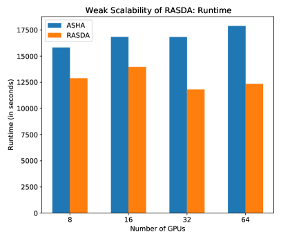
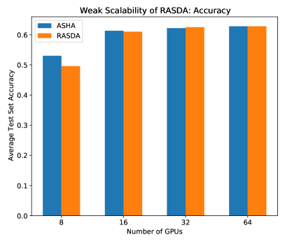
Figure 3: Comparison of ASHA and RASDA for training a ResNet50 model on ImageNet for 20 epochs on different scales on the JURECA-DC-GPU system.

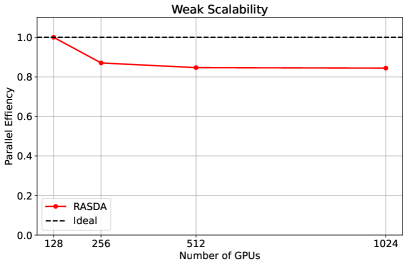
Figure 4: Weak scalability of the RASDA algorithm on up to $1{,}024$ GPUs on the JUWELS BOOSTER system, including ideal scalability for comparison.

5.3 Speed-Ups and Accuracy

To evaluate the performance of the RASDA algorithm in terms of speed-up and accuracy and to juxtapose it to the plain ASHA algorithm considering the application cases, the number of training epochs is increased within the $\min\_t$ and $\max\_t$ range specified in Sec. 4. The general results for the three application case, averaged over three different runs for all application cases, are presented in Tab. 2, Tab. 3, and Tab. 4. The solution quality over time is presented in Fig. 5, an in-depth performance analysis of the runtimes per epoch is given in Fig. 6, and the change of batch size and number of GPUs per trial is depicted in Fig. 7. The results correspond to an exemplary best-performing trial from one of the three runs. The following paragraphs provide a more detailed discussion of these tables and figures.

For the CV application case, a total of 32 hyperparameter combinations are evaluated simultaneously on 64 GPUs on the JURECA-DC-GPU system, with each parallel trial starting with two GPUs. Compared to the plain ASHA approach, the RASDA algorithm reduces the overall average runtime of the HPO process by a factor of $\approx 1.71$ from $527$ to $308$ minutes, see Tab. 2. The average solution quality, i.e., the training, validation, and test set accuracy of the best trial discovered during the process, slightly outperforms the ones of the plain ASHA. This indicates that scaling the batch size and the learning rate during the training process does not impact the learning process in this case. A closer look at one of the best-performing trials in Fig. 6 reveals that indeed the average runtime decreases in the RASDA case once the resource adaptation in space sets in after the first five epochs. As can be seen in Fig. 7, $BS_{global}$ increases from 256 to 2,048 during the training and the number of GPUs from 2 to 16 per trial for the RASDA case, while both stay constant in the plain ASHA case. The plot of the validation accuracy over the number of epochs in Fig. 5 confirms that RASDA slightly outperforms the ASHA approach in terms of solution quality.

For the AM application case, the HPO process evaluates 16 configurations, using a total of 128 GPUs on the JURECA-DC-GPU system. The trials start out with 8 GPUs each, which increases to 32 GPUs for the top-performing trials, at the same time increasing $BS_{global}$ from 64 to 256. As the models are only trained for a total amount of 20 epochs (due to the long training times of transformer models), only two resource-doubling steps, i.e., at epoch 5 and epoch 10, take place, see Fig. 7. Table 3 provides an overview of the results in terms of runtime and solution quality. In comparison with the plain ASHA algorithm, a speed-up by a factor of $1.52$ is achieved, reducing the required HPO runtime of the models from 96 to 63 minutes. On both the validation and test dataset, the best configuration found by RASDA again outperforms the one found with the plain ASHA after 20 epochs, as can be seen in Fig. 5.

The CFD application case features the largest dataset used in this study. The whole HPO process evaluates 16 configurations on 128 GPUs simultaneously on the JUWELS BOOSTER module. Each trial starts with 8 GPUs, which is increased over time to 64 GPU by the RASDA algorithm. As can be seen from Tab. 4, the most significant speed-up with a factor of $\approx 1.9$ is achieved in this case, with RASDA reducing the runtime of the HPO process from 325 to 170 minutes. In this case, also the average MSE decreases by a factor of $\approx 1.88$. This is likely due to the even better generalization capabilities caused by increasing the batch size over time (following the insights explained in Sec. 3.2). Obviously, this outperforms just annealing of the learning rate. This observation is in line with the findings of Smith et al. [44]. RASDA also achieves a low relative reconstruction error of just $1.15\%$ on the test set.

In general, the most substantial speed-up is established on the largest dataset from the CFD domain. This is expected, as with a larger dataset, the benefit of adding more GPUs to the data-parallel training loop also increases. It is additionally interesting to observe that the speed-ups can be attained on both the JURECA-DC-GPU and JUWELS BOOSTER systems, although the latter features twice the network bandwidth. While RASDA already yields substantial benefits on JURECA-DC-GPU with its moderate network infrastructure, the doubled network bandwidth of JUWELS BOOSTER further amplifies these speed-ups, highlighting how the approach particularly profits from fast interconnects.

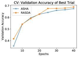
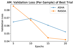
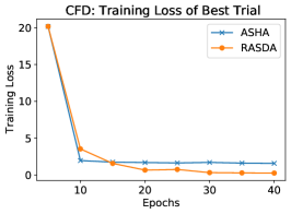
Figure 5: Exemplary comparison of the performance (in terms of validation accuracy, training loss, and validation loss) of the best configuration found by ASHA and RASDA for the different application cases.

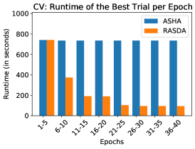
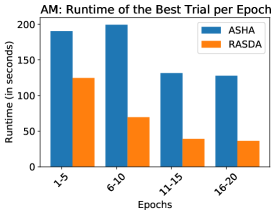
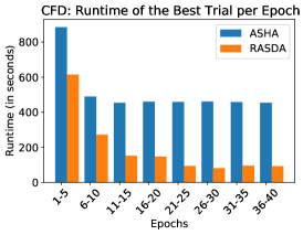
Figure 6: Exemplary comparison of the runtime per epoch of the best configuration found by ASHA and RASDA for the different application cases. Note that for the CFD and AM case, the architectural parameters chosen by the respective HPO method also influence the model size, which is why here differences in runtime can be observed already during the first five epochs.

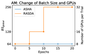
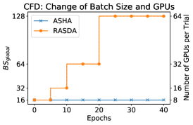
Figure 7: Comparison of the global batch size and the number of GPUs per trial for ASHA and RASDA for the different application cases.

Table 2: HPO for the CV application case, trained for 40 epochs on 64 GPUs on the JURECA-DC-GPU system. Results are averaged over three random seeds. Better results ($\uparrow$ or $\downarrow$ depending on the metric) are underlined.

Metric	ASHA	RASDA	Diff.
Train Accuracy $\uparrow$	0.6976	0.7310	$1.05\times$
Val Accuracy $\uparrow$	0.6728	0.6813	$1.01\times$
Test Accuracy $\uparrow$	0.6688	0.6766	$1.01\times$
Runtime (in seconds) $\downarrow$	31637	18502	$1.71\times$

Table 3: HPO for the AM application case, trained for 20 epochs on 128 GPUs on the JURECA-DC-GPU system. Results are averaged over three random seeds. Better results ($\uparrow$ or $\downarrow$ depending on the metric) are underlined. For better comparison the metrics were recomputed on a per-sample basis after the run.

Metric	ASHA	RASDA	Diff.
Val MSE $\downarrow$	0.0455	0.0404	$1.12\times$
Test MSE $\downarrow$	0.0554	0.0516	$1.07\times$
Runtime (in seconds) $\downarrow$	5784	3803	$1.52\times$

Table 4: HPO for the CFD application case, trained for 40 epochs on 128 GPUs on the JUWELS BOOSTER module. Results are averaged over three random seeds. Better results ($\uparrow$ or $\downarrow$ depending on the metric) are underlined.

Metric	ASHA	RASDA	Diff.
Val MSE $\downarrow$	$5.28\text{\times}{10}^{-06}$	$2.81\text{\times}{10}^{-06}$	$1.88\times$
Test MSE $\downarrow$	$4.42\text{\times}{10}^{-06}$	$2.40\text{\times}{10}^{-06}$	$1.84\times$
Test Relative Error $\downarrow$	0.0185	0.0115	$1.61\times$
Runtime (in seconds) $\downarrow$	19487	10242	$1.90\times$

5.4 Performance at 1,024 GPUs Scale

While the superiority of RASDA over plain ASHA has been confirmed in the previous experiments using 64 and 128 GPUs, a final RASDA experiment on a 1,024 GPU scale is conducted on the JUWELS BOOSTER system. Again, using the CFD application case, the number of configurations to be evaluated is increased to 64, with each trial starting with 16 GPUs. The models are trained for $\min\_t=5$ and $\max\_t=20$ epochs. The HPO run took three hours and resulted in an improved model with a validation MSE of $\approx$3.63\text{\times}{10}^{-07}$$, a test MSE of $\approx$4.88\text{\times}{10}^{-08}$$ and a relative test error of $\approx 0.0016$. Depending on the metric, this is a $7$ to $49$ times increase in solution quality, compared to the results of the HPO run on 128 GPUs (see Tab. 5), which highlights the potential of large-scale HPO for scientific ML.

Table 5: Large-scale HPO for the CFD application case, evaluating $64$ configurations, trained for a maximum of 20 epochs on 1,024 GPUs on the JUWELS BOOSTER module, including relative improvement to the HPO run on 128 GPUs.

Metric	RASDA - 1,024 GPUs	vs. 128 GPUs
Val MSE	$3.63\text{\times}{10}^{-07}$	$7.74\times$
Test MSE	$4.88\text{\times}{10}^{-08}$	$49.22\times$
Test Rel. Error	0.0016	$7.17\times$

6 Summary and Outlook

RASDA, a novel resource-adaptive successive doubling algorithm for HPO, suitable for running on HPC systems, was introduced. The key idea is to not only perform successive halving in time and let promising configurations train for longer (as is already the case in plain ASHA), but to combine it with successive doubling in space and allocate more computational resources to the data-parallel training of promising configurations.

The RASDA method was evaluated extensively on a standard benchmarking task in the CV domain as well as on two large datasets (up to 8.3 TB in size) from the CFD and AM domains. The results confirm that RASDA leads in these cases to speed-ups up to a factor of $\approx 1.9$ in comparison to the ASHA algorithm.

Another property of RASDA is that it progressively scales up the global batch size of the trials as it adds more GPUs to their training loops. This helps them to avoid the degradation in solution quality, which is usually associated with large batch training. Remarkably, the approach did enhance the solution quality, aligning with literature findings suggesting that increasing the batch size can match or surpass the effects of learning rate annealing.

In addition, this study represents the first application of systematic HPO to a scientific dataset at the TB scale. A comparison of the application of RASDA on 128 and 1024 GPUs revealed a significant improvement in model performance. Specifically, the larger-scale application identifies a model that is significantly superior in solution quality. These results demonstrate the scalability and efficiency of the RASDA method, thus paving the way for the application of HPO methods on current and future Exascale supercomputers. For future work, the optimal timing for scaling the batch size (through the addition of more GPUs to the data-parallel training loop) should be investigated more thoroughly. Furthermore, the impact of scaling the batch size on various hyperparameters beyond the learning rate (such as the weight decay values) warrants a deeper exploration.

Conflict of Interest

The authors declare that there are no conflicts of interest related to this work.

Author Contributions

MA: Conceptualization, investigation, methodology, software, visualization, validation, writing - original draft. RS: Methodology, software, validation, writing - review and editing. HN: Supervision, validation, writing - review and editing. MR: Supervision, validation, writing - review and editing. AL: Supervision, validation, writing - review and editing, funding acquisition.

References

- Aach et al. [2023] Aach, M., Sarma, R., Inanc, E., Riedel, M., Lintermann, A., 2023. Short paper: Accelerating hyperparameter optimization algorithms with mixed precision, in: Proceedings of the SC ’23 Workshops of The International Conference on High Performance Computing, Network, Storage, and Analysis, ACM. p. 1776–1779. doi:10.1145/3624062.3624259.
- Aach et al. [2022] Aach, M., Sedona, R., Lintermann, A., Cavallaro, G., Neukirchen, H., Riedel, M., 2022. Accelerating hyperparameter tuning of a deep learning model for remote sensing image classification, in: IGARSS 2022 - 2022 IEEE International Geoscience and Remote Sensing Symposium, IEEE. pp. 263–266. doi:10.1109/IGARSS46834.2022.9883257.
- Akiba et al. [2019] Akiba, T., Sano, S., Yanase, T., Ohta, T., Koyama, M., 2019. Optuna: A next-generation hyperparameter optimization framework, in: Proceedings of the 25th ACM SIGKDD International Conference on Knowledge Discovery & Data Mining, ACM. p. 2623–2631. doi:10.1145/3292500.3330701.
- Albers et al. [2023] Albers, M., Meysonnat, P.S., Fernex, D., Semaan, R., Noack, B.R., Schröder, W., Lintermann, A., 2023. Actuated Turbulent Boundary Layer Flows Dataset. doi:10.34730/5dbc8e35f21241d0889906136cf28d26.
- Balaprakash et al. [2019] Balaprakash, P., Egele, R., Salim, M., Wild, S., Vishwanath, V., Xia, F., Brettin, T., Stevens, R., 2019. Scalable reinforcement-learning-based neural architecture search for cancer deep learning research, in: Proceedings of the International Conference for High Performance Computing, Networking, Storage and Analysis, ACM. doi:10.1145/3295500.3356202.
- Balaprakash et al. [2018] Balaprakash, P., Salim, M., Uram, T.D., Vishwanath, V., Wild, S.M., 2018. Deephyper: Asynchronous hyperparameter search for deep neural networks, in: 2018 IEEE 25th International Conference on High Performance Computing, IEEE. pp. 42–51. doi:10.1109/HiPC.2018.00014.
- Bergstra et al. [2011] Bergstra, J., Bardenet, R., Bengio, Y., Kégl, B., 2011. Algorithms for hyper-parameter optimization, in: Shawe-Taylor, J., Zemel, R., Bartlett, P., Pereira, F., Weinberger, K.Q. (Eds.), Proceedings of the 24th International Conference on Neural Information Processing Systems, Curran Associates, Inc.
- Bergstra and Bengio [2012] Bergstra, J., Bengio, Y., 2012. Random search for hyper-parameter optimization. Journal of Machine Learning Research 13, 281–305. URL: http://jmlr.org/papers/v13/bergstra12a.html.
- Blanc et al. [2023] Blanc, C., Ahar, A., De Grave, K., 2023. Reference dataset and benchmark for reconstructing laser parameters from on-axis video in powder bed fusion of bulk stainless steel. Additive Manufacturing Letters 7, 100161. doi:https://doi.org/10.1016/j.addlet.2023.100161.
- Dunlap et al. [2021] Dunlap, L., Kandasamy, K., Misra, U., Liaw, R., Jordan, M., Stoica, I., Gonzalez, J.E., 2021. Elastic hyperparameter tuning on the cloud, in: Proceedings of the ACM Symposium on Cloud Computing, ACM. p. 33–46. URL: https://doi.org/10.1145/3472883.3486989, doi:10.1145/3472883.3486989.
- Falkner et al. [2018] Falkner, S., Klein, A., Hutter, F., 2018. BOHB: Robust and efficient hyperparameter optimization at scale, in: Proceedings of the 35th International Conference on Machine Learning, PMLR. pp. 1436–1445. URL: https://proceedings.mlr.press/v80/falkner18a.html.
- Feurer and Hutter [2019] Feurer, M., Hutter, F., 2019. Hyperparameter Optimization. Springer International Publishing, Cham. pp. 3–33. doi:10.1007/978-3-030-05318-5_1.
- Glorot and Bengio [2010] Glorot, X., Bengio, Y., 2010. Understanding the difficulty of training deep feedforward neural networks, in: Teh, Y.W., Titterington, M. (Eds.), Proceedings of the Thirteenth International Conference on Artificial Intelligence and Statistics, PMLR. pp. 249–256. URL: https://proceedings.mlr.press/v9/glorot10a.html.
- Goyal et al. [2017] Goyal, P., Dollár, P., Girshick, R., Noordhuis, P., Wesolowski, L., Kyrola, A., Tulloch, A., Jia, Y., He, K., 2017. Accurate, large minibatch sgd: Training imagenet in 1 hour. doi:10.48550/ARXIV.1706.02677, arXiv:1706.02677.
- He et al. [2015] He, K., Zhang, X., Ren, S., Sun, J., 2015. Delving deep into rectifiers: Surpassing human-level performance on imagenet classification, in: Proceedings of the 2015 IEEE International Conference on Computer Vision (ICCV), IEEE. p. 1026–1034. doi:10.1109/ICCV.2015.123.
- He et al. [2016] He, K., Zhang, X., Ren, S., Sun, J., 2016. Deep residual learning for image recognition, in: 2016 IEEE Conference on Computer Vision and Pattern Recognition (CVPR), pp. 770–778. doi:10.1109/CVPR.2016.90.
- Hochreiter and Schmidhuber [1997] Hochreiter, S., Schmidhuber, J., 1997. Flat minima. Neural Comput. 9, 1–42. doi:10.1162/neco.1997.9.1.1.
- Inanc et al. [2023a] Inanc, E., Sarma, R., Aach, M., Lintermann, A., 2023a. AI4HPC. doi:10.5281/zenodo.7705417.
- Inanc et al. [2023b] Inanc, E., Sarma, R., Aach, M., Sedona, R., Lintermann, A., 2023b. AI4HPC: Library to train AI models on HPC systems using CFD datasets, in: Workshop on Advancing Neural Network Training: Computational Efficiency, Scalability, and Resource Optimization (WANT@NeurIPS 2023). URL: https://openreview.net/pdf?id=zQTa2XdPnP.
- Jaderberg et al. [2017] Jaderberg, M., Dalibard, V., Osindero, S., Czarnecki, W.M., Donahue, J., Razavi, A., Vinyals, O., Green, T., Dunning, I., Simonyan, K., Fernando, C., Kavukcuoglu, K., 2017. Population based training of neural networks. arXiv:1711.09846.
- Jamieson and Talwalkar [2016] Jamieson, K., Talwalkar, A., 2016. Non-stochastic best arm identification and hyperparameter optimization, in: Gretton, A., Robert, C.C. (Eds.), Proceedings of the 19th International Conference on Artificial Intelligence and Statistics, PMLR. pp. 240–248. URL: https://proceedings.mlr.press/v51/jamieson16.html.
- Jiang and Balaprakash [2020] Jiang, S., Balaprakash, P., 2020. Graph neural network architecture search for molecular property prediction, in: 2020 IEEE International Conference on Big Data (Big Data), IEEE. pp. 1346–1353. doi:10.1109/BigData50022.2020.9378060.
- Jülich Supercomputing Centre [2021] Jülich Supercomputing Centre, 2021. JUWELS Cluster and Booster: Exascale Pathfinder with Modular Supercomputing Architecture at Juelich Supercomputing Centre. Journal of large-scale research facilities JLSRF 7. doi:10.17815/jlsrf-7-183.
- Jülich Supercomputing Centre [2021] Jülich Supercomputing Centre, 2021. JURECA: Data centric and booster modules implementing the modular supercomputing architecture at Jülich Supercomputing Centre. Journal of large-scale research facilities JLSRF 7. doi:10.17815/jlsrf-7-182.
- Kandasamy et al. [2020] Kandasamy, K., Vysyaraju, K.R., Neiswanger, W., Paria, B., Collins, C.R., Schneider, J., Poczos, B., Xing, E.P., 2020. Tuning hyperparameters without grad students: Scalable and robust bayesian optimisation with dragonfly. Journal of Machine Learning Research 21, 1–27. URL: http://jmlr.org/papers/v21/18-223.html.
- Keskar et al. [2017] Keskar, N.S., Mudigere, D., Nocedal, J., Smelyanskiy, M., Tang, P.T.P., 2017. On large-batch training for deep learning: Generalization gap and sharp minima. doi:10.48550/arXiv.1609.04836, arXiv:1609.04836.
- Kesselheim et al. [2021] Kesselheim, S., Herten, A., Krajsek, K., Ebert, J., Jitsev, J., Cherti, M., Langguth, M., Gong, B., Stadtler, S., Mozaffari, A., Cavallaro, G., Sedona, R., Schug, A., Strube, A., Kamath, R., Schultz, M.G., Riedel, M., Lippert, T., 2021. JUWELS booster – a supercomputer for large-scale AI research, in: Jagode, H., Anzt, H., Ltaief, H., Luszczek, P. (Eds.), High Performance Computing, Springer. pp. 453–468. doi:10.1007/978-3-030-90539-2_31.
- Krizhevsky [2014] Krizhevsky, A., 2014. One weird trick for parallelizing convolutional neural networks. arXiv:1404.5997.
- Li et al. [2018] Li, L., Jamieson, K., DeSalvo, G., Rostamizadeh, A., Talwalkar, A., 2018. Hyperband: A novel bandit-based approach to hyperparameter optimization. Journal of Machine Learning Research 18, 1–52. URL: https://jmlr.org/papers/v18/16-558.html.
- Li et al. [2020a] Li, L., Jamieson, K., Rostamizadeh, A., Gonina, E., Ben-tzur, J., Hardt, M., Recht, B., Talwalkar, A., 2020a. A system for massively parallel hyperparameter tuning, in: Dhillon, I., Papailiopoulos, D., Sze, V. (Eds.), Proceedings of Machine Learning and Systems 2 (MLSys 2020), pp. 230–246. URL: https://proceedings.mlsys.org/paper_files/paper/2020/hash/a06f20b349c6cf09a6b171c71b88bbfc-Abstract.html.
- Li et al. [2020b] Li, S., Zhao, Y., Varma, R., Salpekar, O., Noordhuis, P., Li, T., Paszke, A., Smith, J., Vaughan, B., Damania, P., Chintala, S., 2020b. PyTorch distributed: Experiences on accelerating data parallel training. Proceedings of Very Large Data Base Endowment 13, 3005–3018. doi:10.14778/3415478.3415530.
- Liaw et al. [2019] Liaw, R., Bhardwaj, R., Dunlap, L., Zou, Y., Gonzalez, J.E., Stoica, I., Tumanov, A., 2019. HyperSched: Dynamic resource reallocation for model development on a deadline, in: Proceedings of the ACM Symposium on Cloud Computing, ACM. p. 61–73. doi:10.1145/3357223.3362719.
- Liaw et al. [2018] Liaw, R., Liang, E., Nishihara, R., Moritz, P., Gonzalez, J.E., Stoica, I., 2018. Tune: A research platform for distributed model selection and training. arXiv:1807.05118.
- Lindauer et al. [2022] Lindauer, M., Eggensperger, K., Feurer, M., Biedenkapp, A., Deng, D., Benjamins, C., Ruhkopf, T., Sass, R., Hutter, F., 2022. SMAC3: A versatile bayesian optimization package for hyperparameter optimization. Journal of Machine Learning Research 23, 1–9. URL: http://jmlr.org/papers/v23/21-0888.html.
- Liu et al. [2024] Liu, X., Rüttgers, M., Quercia, A., Egele, R., Pfaehler, E., Shende, R., Aach, M., Schröder, W., Balaprakash, P., Lintermann, A., 2024. Refining computer tomography data with super-resolution networks to increase the accuracy of respiratory flow simulations. Future Generation Computer Systems 159, 474–488. doi:https://doi.org/10.1016/j.future.2024.05.020.
- Loshchilov and Hutter [2017] Loshchilov, I., Hutter, F., 2017. SGDR: Stochastic gradient descent with warm restarts, in: International Conference on Learning Representations. URL: https://openreview.net/pdf?id=Skq89Scxx.
- Malladi et al. [2022] Malladi, S., Lyu, K., Panigrahi, A., Arora, S., 2022. On the SDEs and scaling rules for adaptive gradient algorithms, in: Koyejo, S., Mohamed, S., Agarwal, A., Belgrave, D., Cho, K., Oh, A. (Eds.), Proceedings of the 36th International Conference on Neural Information Processing Systems, Curran Associates, Inc. URL: https://proceedings.neurips.cc/paper_files/paper/2022/file/32ac710102f0620d0f28d5d05a44fe08-Paper-Conference.pdf.
- Mattson et al. [2020] Mattson, P., Cheng, C., Diamos, G., Coleman, C., Micikevicius, P., Patterson, D., Tang, H., Wei, G.Y., Bailis, P., Bittorf, V., Brooks, D., Chen, D., Dutta, D., Gupta, U., Hazelwood, K., Hock, A., Huang, X., Kang, D., Kanter, D., Kumar, N., Liao, J., Narayanan, D., Oguntebi, T., Pekhimenko, G., Pentecost, L., Janapa Reddi, V., Robie, T., St John, T., Wu, C.J., Xu, L., Young, C., Zaharia, M., 2020. MLPerf training benchmark, in: Dhillon, I., Papailiopoulos, D., Sze, V. (Eds.), Proceedings of Machine Learning and Systems, pp. 336–349. URL: https://proceedings.mlsys.org/paper_files/paper/2020/file/411e39b117e885341f25efb8912945f7-Paper.pdf.
- McCandlish et al. [2018] McCandlish, S., Kaplan, J., Amodei, D., Team, O.D., 2018. An empirical model of large-batch training. arXiv:1812.06162.
- Misra et al. [2021] Misra, U., Liaw, R., Dunlap, L., Bhardwaj, R., Kandasamy, K., Gonzalez, J.E., Stoica, I., Tumanov, A., 2021. Rubberband: cloud-based hyperparameter tuning, in: Proceedings of the Sixteenth European Conference on Computer Systems, ACM. p. 327–342. doi:10.1145/3447786.3456245.
- Pata et al. [2024] Pata, J., Wulff, E., Mokhtar, F., Southwick, D., Zhang, M., Girone, M., Duarte, J., 2024. Improved particle-flow event reconstruction with scalable neural networks for current and future particle detectors. Communications Physics 7, 124. doi:10.1038/s42005-024-01599-5.
- Qiao et al. [2021] Qiao, A., Choe, S.K., Subramanya, S.J., Neiswanger, W., Ho, Q., Zhang, H., Ganger, G.R., Xing, E.P., 2021. Pollux: Co-adaptive cluster scheduling for goodput-optimized deep learning, in: 15th USENIX Symposium on Operating Systems Design and Implementation (OSDI 21), USENIX Association. pp. 1–18. URL: https://www.usenix.org/conference/osdi21/presentation/qiao.
- Russakovsky et al. [2015] Russakovsky, O., Deng, J., Su, H., Krause, J., Satheesh, S., Ma, S., Huang, Z., Karpathy, A., Khosla, A., Bernstein, M., Berg, A.C., Fei-Fei, L., 2015. Imagenet large scale visual recognition challenge. International Journal of Computer Vision 115, 211–252. doi:10.1007/s11263-015-0816-y.
- Smith et al. [2018] Smith, S.L., Kindermans, P.J., Le, Q.V., 2018. Don’t decay the learning rate, increase the batch size, in: International Conference on Learning Representations. URL: https://openreview.net/pdf?id=B1Yy1BxCZ.
- Sumbul et al. [2019] Sumbul, G., Charfuelan, M., Demir, B., Markl, V., 2019. Bigearthnet: A large-scale benchmark archive for remote sensing image understanding, in: IGARSS 2019 - 2019 IEEE International Geoscience and Remote Sensing Symposium, IEEE. pp. 5901–5904. doi:10.1109/IGARSS.2019.8900532.
- Taubert et al. [2023] Taubert, O., Weiel, M., Coquelin, D., Farshian, A., Debus, C., Schug, A., Streit, A., Götz, M., 2023. Massively parallel genetic optimization through asynchronous propagation of populations, in: Bhatele, A., Hammond, J., Baboulin, M., Kruse, C. (Eds.), High Performance Computing. ISC High Performance 2023, Springer. pp. 106–124. doi:10.1007/978-3-031-32041-5_6.
- Yang et al. [2023] Yang, Y.Q., Guo, Y.X., Xiong, J.Y., Liu, Y., Pan, H., Wang, P.S., Tong, X., Guo, B., 2023. Swin3d: A pretrained transformer backbone for 3d indoor scene understanding. arXiv:2304.06906.