Gravitational atoms beyond the test field limit:
The case of Sgr A* and ultralight dark matter

Abstract

We construct gravitational atoms including self-gravity, obtaining solutions of the Einstein-Klein-Gordon equations for a scalar field surrounding a non-rotating black hole in a quasi-stationary approximation. We resolve the region near the horizon as well as the far field region. Our results are relevant in a wide range of masses, from ultralight to MeV scalar fields and for black holes ranging from primordial to supermassive. For instance, a system with a scalar field consistent with ultralight dark matter and a black hole mass comparable to that of Sagittarius A* can be modeled. A density spike near the event horizon, although present, is negligible, contrasting with the prediction in [P. Gondolo and J. Silk, Phys. Rev. Lett., 83:1719–1722, 1999] for cold dark matter.

Introduction.—Efforts to disentangle dark matter (DM) properties using direct [1, 2, 3] or indirect [4, 5, 6] detection methods have reported null results, pointing towards the fact that DM may only interact through gravity. Experimental and observational searches have disfavored heavy DM candidates, including massive compact halo objects (MACHOs) and weakly interacting massive particles (WIMPs). This has led to growing interest in lighter DM candidates, often with masses below that of the proton. Examples of these include spin zero particles such as the QCD axion [7, 8, 9, 10], for which $10^{-6}\,\textrm{eV}<m_{a}c^{2}<10^{-3}\,\textrm{eV}$, axion-like particles (ALPs) [11] with masses lighter than the QCD axion, $10^{-26}\,\textrm{eV}<m_{\textrm{ALP}}c^{2}<10^{-6}\,\textrm{eV}$, and fuzzy DM [12], also known as ultralight DM or scalar field (SF) DM [13, 14, 15], where $m_{\textrm{SFDM}}c^{2}\sim 10^{-22}\,\textrm{eV}$.

For scalar light candidates, a rich phenomenology arises when their reduced Compton wavelength $\lambda_{\phi}=\frac{\hbar}{m_{\phi}c}$ ($m_{\phi}$ being the DM particle mass) becomes macroscopic. In previous works [16, 17, 18, 19], we have explored configurations of a SF surrounding a non-rotating black hole (BH), showing that, in the test field approximation they can form quasi-bound states provided that $\lambda_{\phi}$ is larger than twice the Schwarzschild radius $R_{\rm Sch}=\frac{2GM_{BH}}{c^{2}}$, i.e.

$$\left(\frac{4GM_{BH}}{c^{2}}\right)\left(\frac{m_{\phi}c}{\hbar}\right)=\frac{2R_{\rm Sch}}{\lambda_{\phi}}<1\,,$$ (1)

where $M_{BH}$ is the black hole mass. Furthermore, if the left-hand side of Eq. (1) is sufficiently small, this scalar cloud is not radiated away or rapidly swallowed by the BH; on the contrary, it can survive for cosmological times [17]. Moreover, its spectrum resembles that of the hydrogen atom, $(\hbar/m_{\phi}c^{2})\omega_{n}=\sqrt{1-\alpha_{G}^{2}/n^{2}}$ [20, 17, 21], with $\alpha_{G}$ defined in Eq. (2) below. Configurations with these characteristics have been named scalar wigs in [17, 18], and are also known as gravitational atoms in the context of superradiance [22, 23].

By introducing a new set of coordinates that generalize the ingoing Eddington-Finkelstein ones to the self-gravitating case, in this work we further develop the approach of [19] and construct gravitational atoms in spherical symmetry including self-gravity, obtaining quasi-stationary solutions of the Einstein-Klein-Gordon (EKG) equations describing a SF that surrounds a BH.

In terms of the gravitational fine structure constant [24], defined by

$$\alpha_{G}\equiv\frac{GM_{BH}m_{\phi}}{\hbar c}=7.5\times 10^{9}\left(\frac{M_{BH}}{M_{\odot}}\right)\left(\frac{m_{\phi}c^{2}}{\mathrm{eV}}\right),$$ (2)

the condition (1) for the existence of SF clouds in the test field limit becomes $\alpha_{G}<1/4$. Here, given BH and SF masses satisfying this inequality, we obtain a family of solutions parameterized by the SF amplitude $A$ at the horizon. Although the solutions depend on these three parameters, configurations with the same $\alpha_{G}$ and $A$ are related to each other by a simple re-scaling. This facilitates considering a wide set of astrophysical realizations (see Table 1 for relevant examples).

The study of ultralight DM + supermassive BH systems is a long-standing problem [16, 17, 18, 19, 25, 26, 27, 28, 29, 30, 31, 32, 33, 34, 35, 36]. A key challenge in these systems arises from the vastly different scales between the BH and the DM halo core, resulting in configurations with $\alpha_{G}\sim 10^{-6}$ and $R_{\textrm{Sch}}/R_{\textrm{core}}\sim 10^{-10}$. With our model, we can follow very precisely the self-gravitating SF’s behavior from scales many orders of magnitude larger than the BH radius all the way to the apparent horizon, and explore the energy density in the BH’s vicinity even in the strong gravity regime. This allows us, for instance, to study the existence and characteristics of DM spikes [37, 38].

Quasi-stationary model.—We consider a complex SF $\phi$ of mass $m_{\phi}$ minimally coupled to gravity. A key feature that allows us to describe our gravitational atoms accurately is the use of horizon-penetrating coordinates (see also [39, 40] for related work in the context of BHs in cosmology). Specifically, we represent the spherically symmetric spacetime metric as

$$ds^{2}=-a^{2}dt^{2}+dr^{2}+\frac{2m}{r}(adt+dr)^{2}+r^{2}d\Omega^{2},$$ (3)

where $a$ and $m$ are positive functions of the time and areal radial coordinates $(t,r)$, and $d\Omega^{2}$ is the usual line element on the unit two-sphere. In this section only, we use Planck units such that $c=\hbar=G=1$. When $a=1$ and $m$ is constant Eq. (3) reduces to the Schwarzschild metric in the Kerr-Schild form, and the coordinates $(t,r)$ are regular on the future horizon $r=2m$ [41]. In general, the surface $r=2m$ in the spacetime described by the metric (3) is a non-expanding horizon [42], along which the expansion with respect to the outward null vector $(\nabla^{\mu}r)\partial_{\mu}=a^{-1}\partial_{t}$ vanishes.

For the following, we focus on quasi-stationary solutions, for which the SF has the form

$$\phi(t,r)=e^{st}\psi(r),$$ (4)

with $s=\sigma+i\omega$, where $\sigma<0$ is the decay rate and $\omega$ the oscillation frequency. Substituting Eqs. (3,4) into the EKG equations and defining $\gamma:=\sqrt{1+2m/r}$ yields the system

$$\left(1-\frac{2m}{r}\right)\psi^{\prime\prime}=B\psi^{\prime}+C\psi,$$ (5a)

$$2m^{\prime}=e^{2\sigma t}r^{2}\left[\gamma^{2}\left|\frac{s}{a}\psi\right|^{2}+m_{\phi}^{2}|\psi|^{2}+\left(1-\frac{2m}{r}\right)\left|\psi^{\prime}\right|^{2}\right],\qquad$$ (5b)

$$\frac{a^{\prime}}{a}=e^{2\sigma t}r\left|\frac{s}{a}\psi-\psi^{\prime}\right|^{2},$$ (5c)

where a prime denotes derivation with respect to $r$ and

$$B := -\frac{2}{r}\left(1-\frac{m}{r}\right)-\frac{4m}{r}\frac{s}{a}$$ (6a)

$$+ \frac{e^{2\sigma t}r}{\gamma^{2}}\biggl{[}(\gamma^{4}-1)\left|\frac{s}{a}\psi\right|^{2}+\gamma^{2}m_{\phi}^{2}|\psi|^{2}$$

$$+ (1+\gamma^{2})\left(1-\frac{2m}{r}\right)\mbox{Re}\left(\frac{s^{*}}{a}\psi^{*}\psi^{\prime}\right)\biggr{]},$$

$$C := m_{\phi}^{2}+\gamma^{2}\left(\frac{s}{a}\right)^{2}-\frac{2m}{r^{2}}\frac{s}{a}$$ (6b)

$$- e^{2\sigma t}r\biggl{[}\left|\frac{s}{a}\psi\right|^{2}+m_{\phi}^{2}|\psi|^{2}+\left(1-\frac{2m}{r}\right)\left|\psi^{\prime}\right|^{2}$$

$$- \left(1-\frac{2m}{r}\right)\mbox{Re}\left(\frac{s^{*}}{a}\psi^{*}\psi^{\prime}\right)\biggr{]}\frac{s}{a}.$$

Einstein’s equations also yield an equation for the time derivative of $m$ which will not be used in our model. The quasi-stationary approximation consists in replacing the factors $e^{2\sigma t}$ in Eqs. (5b,5c,6) by $1$, such that the metric coefficients $a$ and $m$ can be assumed to be time-independent. After the specification of appropriate boundary conditions at $r=2m$ and $r\to\infty$, the resulting system (5) for $(\psi,m,a)$ constitutes a nonlinear eigenvalue problem for the complex frequency $s$. Their corresponding solutions $(\phi,m,a)$, with $\phi$ given by Eq. (4), yield approximate solutions of the EKG equations which are expected to be accurate on time scales $t\ll t_{0}:=1/|\sigma|$.

At $r\to\infty$ we demand $\psi\to 0$, as required by asymptotic flatness. At $r=2m$ a difficulty arises because the coefficient in front of $\psi^{\prime\prime}$ in Eq. (5a) vanishes there. To treat this problem, we write

$$r=r_{0}(1+z),\quad 2m=r_{0}\left[1+zp(z)\right],$$ (7)

where $r_{0}=2m(r_{0}):=2M_{BH}>0$ is a given parameter which is equal to the apparent horizon radius and $p$ is a positive function of the dimensionless coordinate $z$. Since $1-\frac{2m}{r}=\frac{z}{1+z}(1-p)$ we require that $p<1$ for all $z\geq 0$ in order to avoid the presence of a second horizon in the region $r>r_{0}$. In terms of the new variables $z$ and $p$, Eq. (5a) can be brought into the form

$$z\frac{d^{2}\psi}{dz^{2}}+\Delta(z)\frac{d\psi}{dz}=\Gamma(z)\psi,$$ (8)

with the coefficients $\Delta(z):=-\frac{rB}{1-p}$ and $\Gamma(z):=\frac{r_{0}rC}{1-p}$. If a solution that is regular at $z=0$ exists, then evaluating Eq. (8) at $z=0$ yields

$$\left.\frac{1}{\psi}\frac{d\psi}{dz}\right|_{z=0} = \frac{\Gamma(0)}{\Delta(0)}.$$ (9)

Owing to the factor $1-2m/r$ that multiplies the terms involving $\psi^{\prime}$ in the expressions for $2m^{\prime}$, $B$ and $C$, Eq. (9) can be solved explicitly to determine the first derivative of $\psi$ at $z=0$. Assuming without loss of generality that $a(r_{0})=1$ and noticing that $p(0)=\left.2m^{\prime}\right|_{r=r_{0}}$ can be evaluated using Eq. (5b), one finds

$$p(0) = 2\left(2\alpha_{G}^{2}+\left|\bar{s}\right|^{2}\right)|A|^{2},$$ (10a)

$$\Delta(0) = 1+\frac{4\bar{s}+|\bar{s}|^{2}|A|^{2}}{2(1-p(0))},$$ (10b)

$$\Gamma(0) = \frac{4\alpha_{G}^{2}+2\bar{s}^{2}-\bar{s}-\left(p(0)-\left|\bar{s}\right|^{2}|A|^{2}\right)\bar{s}}{1-p(0)},$$ (10c)

where we have used $r_{0}m_{\phi}=2M_{BH}m_{\phi}=2\alpha_{G}$, and defined $\bar{s}:=r_{0}s$ and $A:=\psi(r_{0})$.

Summarizing, the apparent horizon boundary conditions are

$$\psi(r_{0})=A,\;\;\psi^{\prime}(r_{0})=\frac{A}{r_{0}}\frac{\Gamma(0)}{\Delta(0)},\;\;2m(r_{0})=r_{0},\;\;a(r_{0})=1,$$ (11)

where $\Delta(0)$ and $\Gamma(0)$ are given in Eqs. (10b,10c). Besides $r_{0}=2M_{BH}>0$, the only other free parameter at the horizon is the SF’s amplitude $A$ whose norm should be chosen small enough such that $p(0)<1$. We have assumed that $a(r_{0})=1$ to simplify the calculations; however one can recover the general case by replacing $s$ with $s/a(r_{0})$ in the expressions above. More precise horizon boundary conditions which include an explicit expression for $\psi^{\prime\prime}(r_{0})$ are provided in the supplemental material.

Results.—The solutions are obtained by numerical integration of Eqs. (5) using a shooting algorithm, with boundary conditions at the horizon obtained from Eq. (11), and demanding $\psi\rightarrow 0$ exponentially for large $r$. We concentrate on the ground-state solutions (i.e. those with no zeros of $|\psi(r)|$) and leave the study of the excited states for future work. Some examples are shown in Fig. 1, where the energy density $\rho:=m^{\prime}/(4\pi r^{2})$ and mass function $m$ at $t=0$ are shown for different parameters.

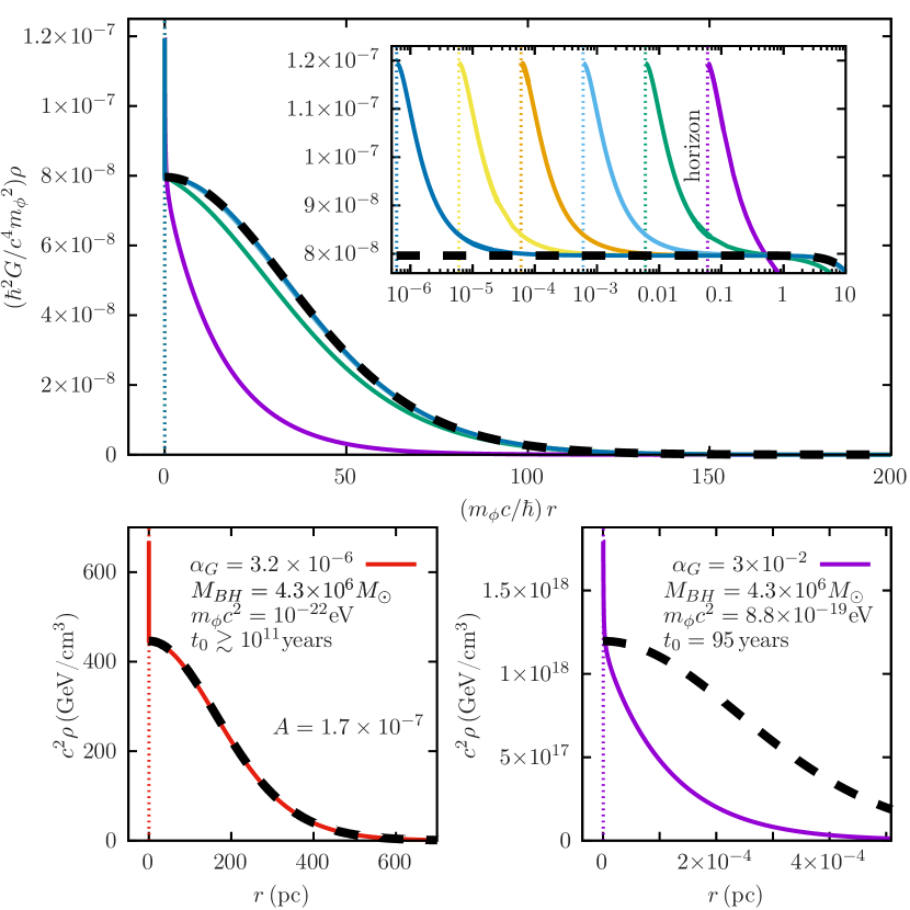
(a) Energy density

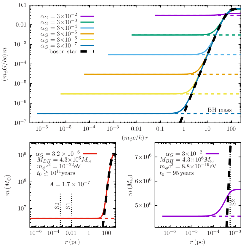
(b) Mass function

Figure 1: Energy density and mass function at $t=0$ for solutions with various values of $\alpha_{G}$, together with those for BSs with the same central amplitude in each case. The amplitude is $A=10^{-3}$ in all cases except the one indicated as $A=1.7\times 10^{-7}$. Color dotted lines in the density plots indicate each apparent horizon’s location, color dashed lines in the mass plots indicate each BH mass, and black dotted lines indicate the pericenter distance of stars S1 and S2 in the case of Sgr A*. The curves belonging to $\alpha_{G}=3{\times}10^{-4}$ to $3{\times}10^{-7}$ are not clearly seen in most of the region because they are superposed almost perfectly with the BS curve.

Let us concentrate first on the top plots in Fig. 1, in which all configurations have $A=10^{-3}$. For small enough $\alpha_{G}$, the solutions (re-scaled by $m_{\phi}$) look very similar to each other and to a boson star (BS) of the same amplitude almost everywhere, except for a very small region close to the horizon, showing a wide core. As $\alpha_{G}$ becomes larger, the solutions begin to differ more and more, displaying a sharper profile. Although it is possible to see an over-density (or spike) [37, 35, 27, 31, 33] near the horizon, its contribution to the mass function is negligible in most cases, even close to the apparent horizon, where $m$ is practically identical to the BH mass. Note that, for fixed $A$, solutions with different values of $\alpha_{G}$ have density spikes with approximately the same height. This is consistent with the fact that at the horizon $8\pi\rho=r_{0}^{2}p_{0}=(m_{\phi}^{2}+2|s|^{2}|)|A|^{2}$, where we have used Eq. (10a), and that $s\approx m_{\phi}$ in these cases.

To exemplify with a particular physical system, we concentrate on Sgr A* setting $M_{BH}=4.3{\times}10^{6}M_{\odot}$, and consider two cases, shown in the bottom plots of Fig. 1, (i) $\alpha_{G}=3.2{\times}10^{-6}$ ($m_{\phi}c^{2}=10^{-22}\mathrm{eV}$), $A=1.7\times 10^{-7}$ and (ii) $\alpha_{G}=3{\times}10^{-2}$ ($m_{\phi}c^{2}=8.8{\times}10^{-19}\mathrm{eV}$), $A=10^{-3}$. We see that the configuration in case (i) is almost identical to a BS with the same parameters, having enough mass to explain the dispersion velocities of bulge stars in spiral galaxies, where supermassive BHs inhabit but play an insignificant role in the galaxy dynamics [44]. S-stars’ trajectories and the BH’s image would be unaffected in this case. On the other hand, in case (ii) the configuration departs strongly from that of a BS. In this case, the SF has a high concentration around the BH. Thus, the contribution of the self-gravitating SF mass in that region is important, and it could even affect the dynamics of S-stars. Note also the huge difference in the characteristic times $t_{0}$ of these configurations. We have $t_{0}\gtrsim 10^{11}\,\mathrm{years}$  in case (i), consistent with galactic lifetimes, and the extremely small value $t_{0}=95\,\mathrm{years}$ in case (ii).

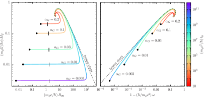
Figure 2: $M_{T}$ vs $R_{99}$ (left panel) and $M_{T}$ vs $\omega$ (right panel) of solutions with various values of $\alpha_{G}$, varying $A$. The color map indicates the characteristic time $t_{0}$. Black dots indicate, for each $\alpha_{G}$, the points where $M_{T}=M_{BH}$, $R_{99}=R_{\rm Sch}$ and $(\hbar/m_{\phi}c^{2})\omega_{n}=\sqrt{1-\alpha_{G}^{2}/n^{2}}$ (with $n=1$). Short vertical lines indicate the locations of the test field’s effective potential minima.

Some solutions’ properties throughout the parameter space are shown in Fig. 2, where the total mass $M_{T}:=m(r\rightarrow\infty)$ is shown as a function of the radius $R_{99}$  and the frequency $\omega$. Each curve is obtained by fixing $\alpha_{G}$ and varying $A$. For small $A$, the test field limit is recovered, at which point the solutions accumulate as $A\rightarrow 0$. The black dots indicate the values $M_{T}=M_{BH}$, $R_{99}=R_{\rm Sch}$ and $(\hbar/m_{\phi}c^{2})\omega_{n}=\sqrt{1-\alpha_{G}^{2}/n^{2}}$ (with $n=1$). As expected, the first two values are recovered for small $A$, whereas the last one is recovered when both $A$ and $\alpha_{G}$ are small enough [18]. In another region of the parameter space, the properties shown become identical to those of BSs, indicated by a dashed line. Note that although this limit occurs at large $A$, it is not necessarily true that it is obtained from $A\rightarrow\infty$ at fixed $\alpha_{G}$. We also see that the characteristic times $t_{0}$, indicated by the color map, span many orders of magnitude.

The condition $\alpha_{G}<1/4$ for the existence of quasi-stationary solutions in the test field limit is recovered empirically for the self-gravitating case, as we were able to find solutions close to, but not beyond that limit. Additionally, for all the solutions obtained in this work, $M_{T}$ is bounded from above by the same value as BSs, that is $(m_{\phi}G/\hbar c)M_{T}<0.633$, with solutions close to this maximum for large enough $A$. In the opposite limit, we have $M_{T}>M_{BH}$, and solutions get close to that minimum for small $A$. Regarding the characteristic time $t_{0}$, we see that it is limited from above by that of the test filed limit for each value of $\alpha_{G}$. This limit can be evaluated in the small $\alpha_{G}$ approximation as shown in [17]. Finally, we provide size estimates. The minimum size in each case is simply given by the Schwarzschild radius, $R_{99}^{\rm min}=R_{\rm Sch}$. Lacking a simple expression for the maximum size, we can provide bounds. An upper bound, $R_{99}^{{\rm max}+}$, is given by the BSs curve, as is evident from Fig. 2. Using the approximation $M_{T}=10\,\hbar^{2}/(Gm_{\phi}^{2}R_{99})$, valid in the non-relativistic limit, we get $R_{99}^{{\rm max}+}=10\,\hbar^{2}/(Gm_{\phi}^{2}M_{BH})$. To estimate a lower bound, $R_{99}^{{\rm max}-}$, we note that the maximum radius is to the right of the test field region. Hence, a lower bound is given by the location of the test field effective potential minimum [18]. Although this is not a very tight bound, it can still be useful for evaluating certain astrophysical scenarios’ plausibility.

Table 1: Limits of $M_{T}$, $R_{99}$ and $t_{0}$ for combinations of $m_{\phi}$ and $M_{BH}$ motivated by various astrophysical scenarios. Note that for $\alpha_{G}>1/4$ there are no solutions, hence those cases are not included. For clarity, we only show orders of magnitude.

$\alpha_{G}$	$m_{\phi}c^{2}$	$M_{BH}=$	$M_{T}^{\rm max}$	$R_{99}^{\rm min}=$	$R_{99}^{{\rm max}-}$	$R_{99}^{{\rm max}+}$	$t_{0}^{\rm max}$	Motivation	Motivation
	(eV)	$M_{T}^{\rm min}\,(M_{\odot})$	$(M_{\odot})$	$R_{\rm Sch}$ (pc)	(pc)	(pc)	(years)	for $m_{\phi}$	for $M_{BH}$
$10^{-29}$	$10^{-22}$	$10^{-17}$	$10^{12}$	$10^{-30}$	$0.1$	$10^{29}$	$10^{144}$	Fuzzy DM	Primordial BH
$10^{-25}$	$10^{-18}$	$10^{-17}$	$10^{8}$	$10^{-30}$	$10^{-5}$	$10^{21}$	$10^{120}$	ALP	Primordial BH
$10^{-25}$	$10^{-22}$	$10^{-13}$	$10^{12}$	$10^{-26}$	$0.1$	$10^{25}$	$10^{124}$	Fuzzy DM	Microlensing limit
$10^{-21}$	$10^{-18}$	$10^{-13}$	$10^{8}$	$10^{-26}$	$10^{-5}$	$10^{17}$	$10^{100}$	ALP	Microlensing limit
$10^{-12}$	$10^{-5}$	$10^{-17}$	$10^{-5}$	$10^{-30}$	$10^{-18}$	$10^{-5}$	$10^{42}$	QCD axion	Primordial BH
$10^{-12}$	$10^{-22}$	$1$	$10^{12}$	$10^{-13}$	$0.1$	$10^{12}$	$10^{59}$	Fuzzy DM	Stellar BH
$10^{-10}$	$10^{-22}$	$100$	$10^{12}$	$10^{-11}$	$0.1$	$10^{10}$	$10^{49}$	Fuzzy DM	LIGO detection
$10^{-8}$	$10^{-5}$	$10^{-13}$	$10^{-5}$	$10^{-26}$	$10^{-18}$	$10^{-9}$	$10^{22}$	QCD axion	Microlensing limit
$10^{-8}$	$10^{-18}$	$1$	$10^{8}$	$10^{-13}$	$10^{-5}$	$10^{4}$	$10^{35}$	ALP	Stellar BH
$10^{-6}$	$10^{-18}$	$100$	$10^{8}$	$10^{-30}$	$10^{-5}$	$100$	$10^{25}$	ALP	LIGO detection
$10^{-6}$	$10^{-22}$	$10^{6}$	$10^{12}$	$10^{-7}$	$0.1$	$10^{6}$	$10^{29}$	Fuzzy DM	Sgr A*
$10^{-3}$	$10^{-22}$	$10^{9}$	$10^{12}$	$10^{-4}$	$0.1$	$10^{3}$	$10^{14}$	Fuzzy DM	M87*
$10^{-2}$	$10^{-18}$	$10^{6}$	$10^{8}$	$10^{-7}$	$10^{-5}$	$10^{-2}$	$10^{5}$	ALP DM	Sgr A*
$10^{-1}$	$10^{6}$	$10^{-17}$	$10^{-16}$	$10^{-30}$	$10^{-29}$	$10^{-27}$	$10^{-24}$	MeV DM	Primordial BH

We now consider some relevant astrophysical examples corresponding to particular values of $M_{BH}$ and $m_{\phi}$ (and hence $\alpha_{G}$), shown in Table 1. The values chosen for $M_{BH}$ are motivated by primordial BHs as dark matter [47], limit BH by micro-lensing [48], stellar BHs, LIGO BH detection [49], Sgr A* [50, 51] and M87*; and those of $m_{\phi}$ by fuzzy DM [12, 13, 14], axion-like particles DM [11], QCD axion DM and MeV DM. Each combination of these sets fixes the two masses, leaving a family of solutions parameterized by $A$ whenever $\alpha_{G}<1/4$, and no solutions otherwise. For the cases with solutions, we show limiting values of $M_{T}$, $R_{99}$, and $t_{0}$ in the table.

Discussion.—The configurations obtained here resemble the quasi-bound states for small values of $A$, while they depart from the hydrogen-like bosonic clouds and yield new self-gravitating configurations for large $A$. In a suitable limit, these configurations approach BSs.

Most configurations display a sort of decoupling, behaving quite differently at different scales. Typically, the relatively small region near the BH (which can however be much larger than the BH itself) has a mass function practically identical to that of the BH alone, whereas at large scale (usually on an extension many orders of magnitude the BH radius) the mass function coincides with that of a BS (without any effect of the central BH).

Of particular interest are cases where the SF is ultralight and the BH is supermassive, for which our solutions are consistent with long-lived DM halo cores with BHs in their center; see examples in Table 1. In particular, the characteristic times of these configurations are larger than cosmological times. In those cases, a density spike is present very close to the apparent horizon. However, its contribution to the mass function is negligible compared to that of the BH, and we do not expect it would alter nearby trajectories significantly. This result contrasts with that reported for cold DM in [37].

Acknowledgments.—This work was partially supported by the CONAHCyT Network Projects No. 376127 “Sombras, lentes y ondas gravitatorias generadas por objetos compactos astrofísico” and No. 304001 “Estudio de campos escalares con aplicaciones en cosmología y astrofísica”, by CONAHCyT-SNII, by PAPIIT-UNAM projects IN100523 and IN110523, by CIC grant No. 18315 of the Universidad Michoacana de San Nicolás de Hidalgo, by the Center for Research and Development in Mathematics and Applications (CIDMA) through the Portuguese Foundation for Science and Technology (FCT - Fundação para a Ciência e a Tecnologia), references UIDB/04106/2020 and UIDP/04106/2020, and by the programme HORIZON-MSCA2021-SE-01 Grant No. NewFun-FiCO101086251. A.D.T. acknowledges support from DAIP project CIIC 2024 198/2024. DN acknowledges the sabbatical support given by PAPIIT-UNAM in the elaboration of the present work. JB, AB, DN and OS thank the Mathematics Department at the University of Aveiro for their hospitality, where part of this work was completed. MM acknowledges financial support from CONICET (PIP 11220210100914CO).

I Supplemental Material

Here, we further develop the apparent horizon boundary conditions and derive an explicit expression for $\psi^{\prime\prime}(r_{0})$. This allows one to start the integration of Eqs. (5) at $r=r_{0}$ and even continue the solution in a small region inside the horizon, which should be useful for numerical evolutions.

Given the central amplitude $A=\psi(r_{0})$ of the field, evaluating Eq. (8) and its first derivative at $z=0$ yields

$$\psi^{\prime}(r_{0}) = \frac{A}{r_{0}}\frac{\Gamma_{0}}{\Delta_{0}},$$ (12)

$$\psi^{\prime\prime}(r_{0}) = \frac{A}{r_{0}^{2}}\frac{\Gamma_{0}^{2}-\Gamma_{0}\Delta_{1}+\Gamma_{1}\Delta_{0}}{\Delta_{0}(1+\Delta_{0})},$$ (13)

with $\Gamma_{k}$ and $\Delta_{k}$ denoting the $k$th order coefficients of

$$\Delta(z):=-\frac{rB}{1-p},\qquad\Gamma(z):=\frac{r_{0}rC}{1-p}$$ (14)

in their Taylor expansion around $z=0$. For the following, we compute these coefficients for $k=0,1$, as needed for Eq. (13).

From Eq. (14), we first obtain

$$\Delta_{0}=-\frac{r_{0}B_{0}}{1-p_{0}},\qquad\Gamma_{0}=-\frac{r_{0}^{2}C_{0}}{1-p_{0}},$$ (15)

$$\Delta_{1}=-\frac{r_{0}}{1-p_{0}}\left(B_{1}+\frac{1-p_{0}+p_{1}}{1-p_{0}}\,B_{0}\right),$$ (16)

$$\Gamma_{1}=\frac{r_{0}^{2}}{1-p_{0}}\left(C_{1}+\frac{1-p_{0}+p_{1}}{1-p_{0}}\,C_{0}\right),$$ (17)

where $p_{k}$, $B_{k}$ and $C_{k}$ refer again to the Taylor coefficients at $z=0$. Evaluating Eqs. (6a,6b) at $z=0$ one first finds

$$r_{0}B_{0} =-\left[1+2\bar{s}-\left(8{\alpha_{G}}^{2}+3|\bar{s}|^{2}\right)\frac{|A|^{2}}{2}\right],$$ (18)

$$r_{0}^{2}C_{0} =4{\alpha_{G}}^{2}+2|\bar{s}|^{2}-\bar{s}\,\left[1+\left(4{\alpha_{G}}^{2}+|\bar{s}|^{2}\right)|A|^{2}\right],$$ (19)

where we recall the definitions $\bar{s}:=r_{0}s$ and $\alpha_{G}=r_{0}m_{\phi}/2$. Together with the expression for $p_{0}$ in Eq. (10a) this yields the results for $\Delta_{0}$ and $\Gamma_{0}$ listed in Eqs. (10b,10c).

Next, in order to compute $p_{1}$, we differentiate Eq. (7) twice and evaluate at $z=0$, which yields $p_{1}=r_{0}\left.m^{\prime\prime}\right|_{r=r_{0}}$. To evaluate the second derivative of $m$, we use Eq. (5b) together with the following identities which can be inferred from Eqs. (7,5c) and the definition of $\gamma$:

$$\left.(\gamma^{2})^{\prime}\right|_{r=r_{0}}=\frac{p_{0}-1}{r_{0}},\qquad\left.a^{\prime}\right|_{r=r_{0}}=\frac{1}{r_{0}}\left|\bar{s}-T_{0}\right|^{2}|A|^{2},$$ (20)

where we have introduced $T_{0}:=\Gamma_{0}/\Delta_{0}$ to simplify the notation. This yields

$$p_{1} = \frac{p_{0}}{2}\left(2+T_{0}+T_{0}^{*}\right)+\frac{1}{2}(p_{0}-1)\left(|\bar{s}|^{2}-|T_{0}|^{2}\right)|A|^{2}$$ (21)

$$- 2|\bar{s}|^{2}\left|\bar{s}-T_{0}\right|^{2}|A|^{4}.$$

Finally, differentiating Eqs. (6a,6b) and using the identities (20) again one obtains

$$r_{0}B_{1} = h_{a}\,|T_{0}|^{2}+h_{b}\,T_{0}+h_{c}\,T_{0}^{*}+h_{d},$$ (22)

$$r_{0}^{2}C_{1} = j_{a}\,|T_{0}|^{2}+j_{b}\,T_{0}+j_{c}\,T_{0}^{*}+j_{d},$$ (23)

with coefficients

$$h_{a} = \bar{s}\,|A|^{2}\,\left(2-3\,\bar{s}^{*}\,|A|^{2}\right),$$

$$h_{b} = -\frac{|A|^{2}}{4}\,\left[6\,|A|^{2}\,\bar{s}^{*}\,\left(2\,{\alpha_{G}}^{2}-|\bar{s}|^{2}\right)-16\,{\alpha_{G}}^{2}+\right.$$

$$\left.2\,|\bar{s}|^{2}-3\,\bar{s}^{*}\right],$$

$$h_{c} = -\frac{|A|^{2}}{4}\,\left[6\,|A|^{2}\,\bar{s}\,\left(2\,{\alpha_{G}}^{2}-|\bar{s}|^{2}\right)-16\,{\alpha_{G}}^{2}+8\,\bar{s}^{2}\right.$$

$$\left.-6\,|\bar{s}|^{2}-3\,\bar{s}\right],$$

$$h_{d} = \frac{|A|^{4}\,|\bar{s}|^{2}}{2}\,\left(10\,{\alpha_{G}}^{2}-\,|\bar{s}|^{2}\right)+2\bar{s}+$$

$$|A|^{2}\,\left[8\,{\alpha_{G}}^{2}\,\left(1-|\bar{s}|^{2}\right)+|\bar{s}|^{2}\,\left(\frac{9}{4}-2\bar{s}\right)\right],$$

$$j_{a} = \bar{s}\,|A|^{2}\,\left[|A|^{2}\,\left(8\,{\alpha_{G}}^{2}+5\,|\bar{s}|^{2}\right)-4\,\bar{s}^{*}\right],$$ (24)

$$j_{b} = -\frac{|A|^{2}\,\bar{s}}{2}\left[4\,|A|^{2}\,\bar{s}^{*}\,\left(3\,{\alpha_{G}}^{2}+2\,|\bar{s}|^{2}\right)+\right.$$

$$\left.2\,\left(4\,{\alpha_{G}}^{2}+|\bar{s}|^{2}-4\,\left(\bar{s}^{*}\right)^{2}\right)+\bar{s}^{*}\right],$$

$$j_{c} = -\frac{|A|^{2}\,\bar{s}}{2}\left[4\,|A|^{2}\,\bar{s}\,\left(3\,{\alpha_{G}}^{2}+2\,|\bar{s}|^{2}\right)+\right.$$

$$\left.8\,{\alpha_{G}}^{2}-6\,|\bar{s}|^{2}+\bar{s}\right],$$

$$j_{d} = \bar{s}\,\left[|A|^{4}\,|\bar{s}|^{2}\,\left(4\,{\alpha_{G}}^{2}+3\,|\bar{s}|^{2}\right)+\right.$$

$$\left.2\,|A|^{2}\,\left(2\,{\alpha_{G}}^{2}\,\bar{s}^{*}-\bar{s}^{*}\,|\bar{s}|^{2}-4\,{\alpha_{G}}^{2}-|\bar{s}|^{2}\right)-\bar{s}^{*}+2\right].$$

References

- [1] Yue Meng et al. Dark Matter Search Results from the PandaX-4T Commissioning Run. Phys. Rev. Lett., 127(26):261802, 2021.
- [2] J. Aalbers et al. First Dark Matter Search Results from the LUX-ZEPLIN (LZ) Experiment. Phys. Rev. Lett., 131(4):041002, 2023.
- [3] E. Aprile et al. First Dark Matter Search with Nuclear Recoils from the XENONnT Experiment. Phys. Rev. Lett., 131(4):041003, 2023.
- [4] Deheng Song, Kohta Murase, and Ali Kheirandish. Constraining decaying very heavy dark matter from galaxy clusters with 14 year Fermi-LAT data. JCAP, 03:024, 2024.
- [5] Man Ho Chan, Lang Cui, Jun Liu, and Chun Sing Leung. Ruling out GeV thermal relic annihilating dark matter by radio observation of the Andromeda galaxy. Astrophys. J., 872(2):177, 2019.
- [6] Rahool Kumar Barman, Geneviève Bélanger, Biplob Bhattacherjee, Rohini M. Godbole, and Rhitaja Sengupta. Is Light Neutralino Thermal Dark Matter in the Phenomenological Minimal Supersymmetric Standard Model Ruled Out? Phys. Rev. Lett., 131(1):011802, 2023.
- [7] R. D. Peccei and Helen R. Quinn. CP Conservation in the Presence of Instantons. Phys. Rev. Lett., 38:1440–1443, 1977.
- [8] L. F. Abbott and P. Sikivie. A Cosmological Bound on the Invisible Axion. Phys. Lett. B, 120:133–136, 1983.
- [9] Michael Dine and Willy Fischler. The Not So Harmless Axion. Phys. Lett. B, 120:137–141, 1983.
- [10] John Preskill, Mark B. Wise, and Frank Wilczek. Cosmology of the Invisible Axion. Phys. Lett. B, 120:127–132, 1983.
- [11] David J. E. Marsh. Axion Cosmology. Phys. Rept., 643:1–79, 2016.
- [12] Wayne Hu, Rennan Barkana, and Andrei Gruzinov. Cold and fuzzy dark matter. Phys. Rev. Lett., 85:1158–1161, 2000.
- [13] Tonatiuh Matos, Francisco Siddhartha Guzman, and L. Arturo Urena-Lopez. Scalar field as dark matter in the universe. Class. Quantum Grav., 17:1707–1712, 2000.
- [14] Tonatiuh Matos and L. Arturo Urena-Lopez. A Further analysis of a cosmological model of quintessence and scalar dark matter. Phys. Rev. D, 63:063506, 2001.
- [15] Lam Hui, Jeremiah P. Ostriker, Scott Tremaine, and Edward Witten. Ultralight scalars as cosmological dark matter. Phys. Rev. D, 95(4):043541, 2017.
- [16] Juan Barranco, Argelia Bernal, Juan Carlos Degollado, Alberto Diez-Tejedor, Miguel Megevand, Miguel Alcubierre, Dario Nunez, and Olivier Sarbach. Are black holes a serious threat to scalar field dark matter models? Phys. Rev. D, 84:083008, 2011.
- [17] Juan Barranco, Argelia Bernal, Juan Carlos Degollado, Alberto Diez-Tejedor, Miguel Megevand, Miguel Alcubierre, Dario Nunez, and Olivier Sarbach. Schwarzschild black holes can wear scalar wigs. Phys. Rev. Lett., 109:081102, 2012.
- [18] Juan Barranco, Argelia Bernal, Juan Carlos Degollado, Alberto Diez-Tejedor, Miguel Megevand, Miguel Alcubierre, Darío Núñez, and Olivier Sarbach. Schwarzschild scalar wigs: spectral analysis and late time behavior. Phys. Rev. D, 89(8):083006, 2014.
- [19] Juan Barranco, Argelia Bernal, Juan Carlos Degollado, Alberto Diez-Tejedor, Miguel Megevand, Dario Nunez, and Olivier Sarbach. Self-gravitating black hole scalar wigs. Phys. Rev. D, 96(2):024049, 2017.
- [20] Steven L. Detweiler. Klein-Gordon equation and rotating black holes. Phys. Rev. D, 22:2323–2326, 1980.
- [21] Sam R. Dolan. Instability of the massive Klein-Gordon field on the Kerr spacetime. Phys. Rev. D, 76:084001, 2007.
- [22] Daniel Baumann, Horng Sheng Chia, John Stout, and Lotte ter Haar. The Spectra of Gravitational Atoms. JCAP, 12:006, 2019.
- [23] Daniel Baumann, Gianfranco Bertone, John Stout, and Giovanni Maria Tomaselli. Ionization of gravitational atoms. Phys. Rev. D, 105(11):115036, 2022.
- [24] Asimina Arvanitaki, Masha Baryakhtar, and Xinlu Huang. Discovering the QCD Axion with Black Holes and Gravitational Waves. Phys. Rev. D, 91(8):084011, 2015.
- [25] Luis Arturo Urena-Lopez and Andrew R. Liddle. Supermassive black holes in scalar field galaxy halos. Phys. Rev. D, 66:083005, 2002.
- [26] Alejandro Cruz-Osorio, F. Siddhartha Guzman, and Fabio D. Lora-Clavijo. Scalar Field Dark Matter: behavior around black holes. JCAP, 06:029, 2011.
- [27] Elliot Yarnell Davies and Philip Mocz. Fuzzy Dark Matter Soliton Cores around Supermassive Black Holes. Mon. Not. Roy. Astron. Soc., 492(4):5721–5729, 2020.
- [28] Nitsan Bar, Kfir Blum, Thomas Lacroix, and Paolo Panci. Looking for ultralight dark matter near supermassive black holes. JCAP, 07:045, 2019.
- [29] Lam Hui, Daniel Kabat, Xinyu Li, Luca Santoni, and Sam S. C. Wong. Black Hole Hair from Scalar Dark Matter. JCAP, 06:038, 2019.
- [30] Katy Clough, Pedro G. Ferreira, and Macarena Lagos. Growth of massive scalar hair around a Schwarzschild black hole. Phys. Rev. D, 100(6):063014, 2019.
- [31] Zhi Li, Juntai Shen, and Hsi-Yu Schive. Testing the Prediction of Fuzzy Dark Matter Theory in the Milky Way Center. 1 2020.
- [32] Vitor Cardoso, Taishi Ikeda, Rodrigo Vicente, and Miguel Zilhão. Parasitic black holes: The swallowing of a fuzzy dark matter soliton. Phys. Rev. D, 106(12):L121302, 2022.
- [33] Reggie C. Pantig and Ali Övgün. Black Hole in Quantum Wave Dark Matter. Fortsch. Phys., 71(1):2200164, 2023.
- [34] Josu C. Aurrekoetxea, Katy Clough, Jamie Bamber, and Pedro G. Ferreira. Effect of Wave Dark Matter on Equal Mass Black Hole Mergers. Phys. Rev. Lett., 132(21):211401, 2024.
- [35] Riccardo Della Monica and Ivan de Martino. Bounding the mass of ultralight bosonic dark matter particles with the motion of the S2 star around Sgr A*. Phys. Rev. D, 108(10):L101303, 2023.
- [36] Josu C. Aurrekoetxea, James Marsden, Katy Clough, and Pedro G. Ferreira. Self-interacting scalar dark matter around binary black holes. Phys. Rev. D, 110(8):083011, 2024.
- [37] Paolo Gondolo and Joseph Silk. Dark matter annihilation at the galactic center. Phys. Rev. Lett., 83:1719–1722, 1999.
- [38] Laleh Sadeghian, Francesc Ferrer, and Clifford M. Will. Dark matter distributions around massive black holes: A general relativistic analysis. Phys. Rev. D, 88(6):063522, 2013.
- [39] Sarah Chadburn and Ruth Gregory. Time dependent black holes and scalar hair. Class. Quantum Grav., 31(19):195006, October 2014.
- [40] Ruth Gregory, David Kastor, and Jennie Traschen. Evolving Black Holes in Inflation. Class. Quantum Grav., 35(15):155008, 2018.
- [41] Subrahmanyan Chandrasekhar. The mathematical theory of black holes. 1985.
- [42] A. Ashtekar and B. Krishnan. Isolated and dynamical horizons and their applications. Living Reviews in Relativity, 7(1):10, 2004.
- [43] See Supplemental Material at [URL] for more details on the boundary conditions.
- [44] Ivan De Martino, Tom Broadhurst, S. H. Henry Tye, Tzihong Chiueh, and Hsi-Yu Schive. Dynamical Evidence of a Solitonic Core of in the Milky Way. Phys. Dark Univ., 28:100503, 2020.
- [45] In this case is many orders of magnitude smaller than , which makes it difficult to obtain its value accurately. We are still able to obtain an approximate upper bound, and hence an approximate lower bound for .
- [46] As usual, we define the radius as that of a sphere containing of the total mass.
- [47] Bernard Carr and Florian Kuhnel. Primordial Black Holes as Dark Matter: Recent Developments. Ann. Rev. Nucl. Part. Sci., 70:355–394, 2020.
- [48] Hiroko Niikura et al. Microlensing constraints on primordial black holes with Subaru/HSC Andromeda observations. Nature Astron., 3(6):524–534, 2019.
- [49] B. P. Abbott et al. Observation of Gravitational Waves from a Binary Black Hole Merger. Phys. Rev. Lett., 116(6):061102, 2016.
- [50] R. Schodel et al. A Star in a 15.2 year orbit around the supermassive black hole at the center of the Milky Way. Nature, 419:694–696, 2002.
- [51] A. M. Ghez et al. Measuring Distance and Properties of the Milky Way’s Central Supermassive Black Hole with Stellar Orbits. Astrophys. J., 689:1044–1062, 2008.