\ul
Scalable Multi-Objective Reinforcement Learning with Fairness Guarantees using Lorenz Dominance
Abstract
Multi-Objective Reinforcement Learning (MORL) aims to learn a set of policies that optimize trade-offs between multiple, often conflicting objectives. MORL is computationally more complex than single-objective RL, particularly as the number of objectives increases. Additionally, when objectives involve the preferences of agents or groups, ensuring fairness is socially desirable. This paper introduces a principled algorithm that incorporates fairness into MORL while improving scalability to many-objective problems. We propose using Lorenz dominance to identify policies with equitable reward distributions and introduce -Lorenz dominance to enable flexible fairness preferences. We release a new, large-scale real-world transport planning environment and demonstrate that our method encourages the discovery of fair policies, showing improved scalability in two large cities (Xi’an and Amsterdam). Our methods outperform common multi-objective approaches, particularly in high-dimensional objective spaces.
1 Introduction
Reinforcement Learning (RL) is a powerful framework for sequential decision-making, in which agents learn to maximize long-term rewards by interacting with an environment (?). In typical RL applications, rewards are formalized by combining multiple criteria (or objectives) into a single scalar value, by weighting them (?). This approach, however, assumes prior knowledge of precise preferences over these objectives, which may not always be available in real-world scenarios. Additionally, real-world problems often involve multiple, often conflicting objectives. Defining a scalar reward function prior to training can bias the decision-making process, potentially overlooking valuable policies that vary primarily in how these objectives are weighted (?).
Multi-Objective Reinforcement Learning (MORL) addresses this challenge by introducing a distinct reward function for each objective (?). This results in a set of candidate optimal policies, rather than a single solution, allowing decision-makers to select policies based on their private preferences. MORL has been successfully applied to various domains, including decision-making under unknown preferences (?, ?), human-value alignment (?, ?), robot locomotion (?), and multi-agent systems (?, ?, ?).
Multi-policy methods in MORL address situations with unknown preference settings by assuming a monotonically increasing utility function and optimizing for all objectives simultaneously, approximating the Pareto front of optimal, efficient policies (?, ?, ?). However, even with this minimal assumption, the solution set scales exponentially with the number of objectives, a challenge that is particularly pronounced in many-objective optimization, where the problem involves many different objectives (?, ?). As a result, multi-policy methods often struggle to scale efficiently in such scenarios, underscoring the importance of further research in many-objective optimization within RL (?).
Furthermore, learning the complete Pareto front of a problem is often unnecessary, as certain policies may be inherently undesirable (?). For example, in fairness-critical applications, some Pareto-non-dominated policies may lead to inequitable reward distributions between different objectives, which is particularly undesirable when objectives represent the utilities of different societal groups or people (?, ?). Although egalitarian approaches, such as maxmin or equal weighting can address this, they assume a predefined exact preference over the different objectives, often limiting flexibility and can sometimes result in inefficient solutions (?). This reveals a research gap in MORL: no current multi-policy method (a) provides fairness guarantees to the decision-maker, (b) allows control over the fairness constraint, and (c) scales effectively to problems with many objectives.
In this paper, we propose leveraging Lorenz dominance to identify a subset of the Pareto front that ensures equitable reward distribution without predefined preferences. We extend this approach with -Lorenz dominance, which allows decision-makers to adjust the strictness of fairness constraints via a parameter . We formally demonstrate that -Lorenz dominance enables interpolation between Lorenz and Pareto dominance, offering decision-makers fine-grained control over fairness constraints. Furthermore, we introduce Lorenz Conditioned Networks (LCN), a novel algorithm designed to optimize for -Lorenz dominance.
To support scalability in many-objective settings, we design a new large-scale, multi-objective environment for planning transport networks in real-world cities with a flexible number of objectives. We conducted experiments in the cities of Xi’an (China) and Amsterdam (Netherlands) and show that LCN generates fair policy sets in large objective spaces. As Lorenz-optimal sets are generally smaller than Pareto-optimal sets (?), LCN exhibits excellent scalability, especially for many-objective problems.
Alongside the paper, we release the code and data used to generate our results 111Github repository: https://github.com/sias-uva/mo-transport-network-design.
2 Related Work
Our work lies at the intersection of multi-policy methods for MORL (?) and algorithmic fairness in sequential decision-making problems (?).
2.1 Multi-Policy MORL
Early multi-policy methods in reinforcement learning (RL) used Pareto Q-learning, which was mainly limited to small-scale environments (?, ?, ?). To address scalability, many approaches assume that decision makers have linear preferences, leading to a simpler solution set known as the convex coverage set (?, ?, ?). For example, GPI-LS, a state-of-the-art method against which we compare our method, decomposes the multi-objective problem into single-objective subproblems in which the reward function is a convex combination of the original vectorial reward and subsequently trains a neural network to approximate the optimal policies under different weights (?). Beyond linear preferences, the Iterated Pareto Referent Optimisation (IPRO) method takes a similar decomposition-based approach and provides strong theoretical guarantees but was shown to suffer when increasing the number of objectives (?). In contrast, Pareto Conditioned Networks (PCNs) do not decompose the problem, but instead train a return-conditioned policy(?, ?, ?). Similarly, PD-MORL approximates the Pareto front by uniformly sampling preferences across the preference space (?). We propose a method inspired by PCNs that focuses on fairness, avoiding the need to search the entire preference space. This allows for scalability to higher dimensions while learning a set of fair policies, and offers flexibility in setting fairness preferences.
2.2 Fairness in MORL
Research on fairness in RL can be categorized along two main themes (?): fairness in domains where individuals belong to protected groups (societal bias) and fairness in resource allocation problems (non-societal bias). Our work aligns closely with the first theme, focusing on the fair distribution of benefits among different societal groups. Group fairness has been studied in RL before, specifically in multi-agent scenarios (?, ?), where agents learn individual policies. Although here we focus on single-agent RL, we assume that the policies learned by the agent will impact groups of individuals, possibly with conflicting preferences.
Fairness in RL often involves balancing multiple objectives. Many studies in this area incorporate diverse objectives into a single fairness-based reward function. This is typically achieved through linear reward scalarization (?, ?, ?), generalization to nonlinear combinations of rewards, and welfare functions such as the Generalized Gini Index (?, ?, ?), as well as other reward-shaping mechanisms (?, ?, ?, ?). Alternatively, some methods modify the reward function during training to comply with fairness constraints (?). These approaches require encoding the desired fairness principles into the reward functions beforehand, requiring preferential information prior to training. Our approach does not make such assumptions.
Our work is closely related to (?), who propose a formal MORL fairness framework that encodes six fairness notions as objectives. They train PCN to identify Pareto-optimal trade-offs between these fairness notions. Although our method can be applied within this framework, it differs in that it does not precalculate any specific fairness notion. Instead, it learns a set of non-dominated policies across all objectives, allowing the decision-maker to define their criteria post-training. While Lorenz-dominance has previously been used in multi-objective optimization methods (?, ?), this paper is the first attempt to use its properties to learn multiple policies in MORL.
3 Preliminaries
In this section, we formally introduce multi-objective reinforcement learning and the fairness criterion we focus on.
3.1 Multi-Objective Reinforcement Learning
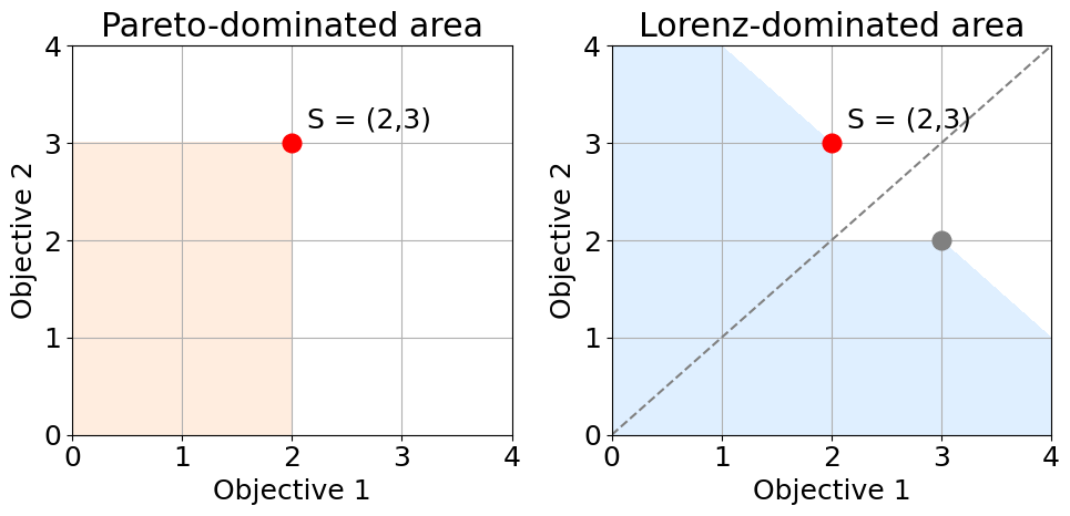
We consider reinforcement learning agents that interact with aMulti-Objective Markov Decision Process (MOMDP). MOMDPs are represented as a tuple consisting of a set of states , set of actions , transition function , vector-based reward function , with the number of objectives, and a discount factor . To act in an MOMDP, we consider deterministic policies mapping states to actions. When the reward is vector-based, there is generally not a single optimal policy and we instead consider learning a set of optimal policies using some dominance criterion. In particular, it is common in MORL to apply Pareto dominance, formally defined below, resulting in a solution set known as the Pareto front.
Definition 1.
(Pareto dominance) Consider two vectors . We say that Pareto dominates , denoted , when and .
In essence, Pareto dominates when it is at least equal in all objectives and better in at least one. For a set of vectors , the Pareto front contains all vectors that are non-Pareto dominated.
3.2 Fairness in Many-Objective Reinforcement Learning
One common fairness approach in multi-objective reinforcement learning (MORL) is to treat all objectives as equally important, optimizing a single, equally weighted objective. However, this assumes absolute equality in reward distribution, which may be infeasible in certain problems, and yields a single policy, without offering options to the decision-maker. Another approach, inspired by Rawlsian justice theory and the maxmin principle, focuses on maximizing the minimum reward between objectives. However, this often results in solutions that are not fully efficient for all users (?).
To train a multi-policy algorithm with fair trade-offs, it is necessary to identify all optimal trade-offs that achieve a fair distribution of rewards. To achieve this, we use Lorenz dominance, a refinement of Pareto dominance that considers the distribution of values within a vector (?). This concept, traditionally used in economics to assess income inequality (?), is adapted here for fairness in MORL.
Definition 2.
(Lorenz dominance) Let be the Lorenz vector of a vector , defined as follows:
| (1) |
where are the values of the vector , sorted in increasing order. A vector Lorenz dominates a vector , when its Lorenz vector Pareto dominates the Lorenz vector (?).
Our fairness criterion seeks Pareto-optimal trade-offs that distribute rewards fairly across objectives, without encoding this preference explicitly into a scalarization function. This approach generates a set of trade-offs, allowing the decision-maker to select the most appropriate one after training. Lorenz-based fairness is grounded in the Pigou-Dalton transfer principle from economics (?, ?). For a vector with for some , a transfer of any () to create , where and are indicator vectors for the th and th elements, respectively, results in a preferred distribution of rewards while preserving the total sum (?). Consider, for example, vector . If we perform a transfer of , the new vector is more desirable under Lorenz-fairness, since the reward is distributed equally between the two dimensions, while the total sum remains the same.
In MORL, we define vectors as the expected return of the policies , across all objectives of the environment, respectively. We define fair policies as those that are non-Lorenz dominated. The set of non-dominated value vectors is called a Lorenz coverage set, which is usually (but not necessarily) significantly smaller than a Pareto coverage set (?). Our fairness approach satisfies the criteria outlined by ?. It is Lorenz-efficient as the learned policies are non-Lorenz-dominated; it is impartial, since it treats all objectives as equally important, and it is equitable, as Lorenz dominance satisfies the Pigou-Dalton principle (?). In Figure 1, we show the difference between Pareto and Lorenz dominance. The latter extends the are of undesired solutions, allowing for fewer non-dominated solutions and providing fairness guarantees in the two objectives.
4 Flexible Fairness with -Lorenz Dominance
To give decision-makers fine-grained control over the fairness needs of their specific problem, we introduce a novel criterion, called -Lorenz dominance. -Lorenz dominance operates on the return vectors directly, rather than introducing a weighting over the objectives (such as the Generalized Gini Index (?)). Furthermore, by selecting a single parameter , -Lorenz dominance allows decision-makers to balance Pareto optimality and Lorenz optimality. We formally define -Lorenz dominance in Definition 3.
Definition 3 (-Lorenz dominance).
Let be the vector sorted in increasing order. Given , a vector -Lorenz dominates another vector , denoted if,
| (2) |
Intuitively, for , it is assumed that the decision-maker cares equally about all objectives and thus may reorder them. This ensures that vectors that were not Pareto-dominated can become dominated. Consider, for example, and . While no vector is Pareto dominated, reordering the objectives in increasing order leads to and and therefore allows ignoring the second vector. This approach may already reduce the size of the Pareto front, but does not yet achieve the same fairness constraints imposed by the Lorenz front. Setting ensures that the solution set is equal to the Lorenz front.
The -Lorenz front of a given set , denoted contains all vectors which are pairwise non -Lorenz dominated. In Theorem 1 we show that, by decreasing , the solution set smoothly converges to the Lorenz front. The detailed proof can be found in the supplementary material.
Theorem 1.
and the following relations hold.
| (3) |
Proof sketch.
To prove Theorem 1, we provide three auxiliary results. First, we demonstrate that for all parameters and vectors we have that:
| (4) |
Together with some algebra, this result is subsequently used to show that for all parameters and such that ,
| (5) |
Finally, we extend a previous result from ? to show that Pareto dominance implies -Lorenz dominance as well. These components are combined to obtain the desired result. ∎
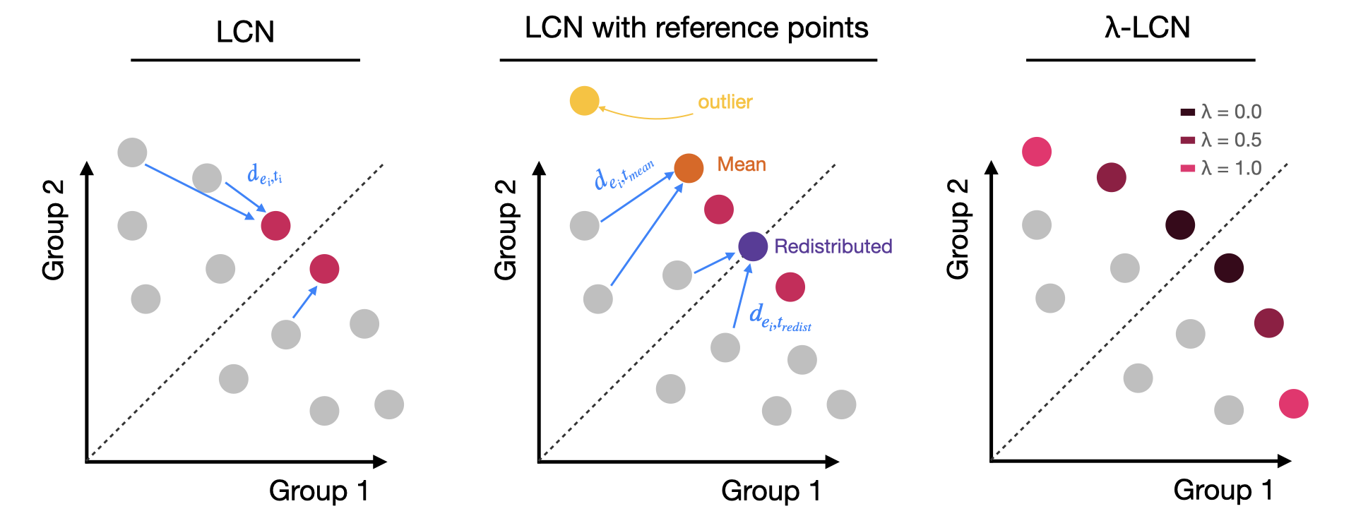
It is a straightforward corollary that for while for . In Figure 2 (right) we illustrate conceptually how the controls the size of the coverage set to consider.
5 Lorenz Conditioned Networks
We introduce Lorenz Conditioned Networks (LCNs), an adaptation of PCNs aimed at learning a -Lorenz front. We then identify a significant drawback in PCN’s management of the ER buffer (Section 5.4) and propose the use of reference points to mitigate ER volatility.
LCNs belong to the class of conditioned networks, also referred to as inverse reinforcement learning (IRL), where a policy is trained as a single neural network through supervised learning (?, ?). This policy maps states and desired rewards to probability distributions over actions by using collected experiences—taking actions as labels and states/rewards as inputs. In a multi-objective setting, the network learns multiple policies, each representing a Lorenz-optimal trade-off.
5.1 Network
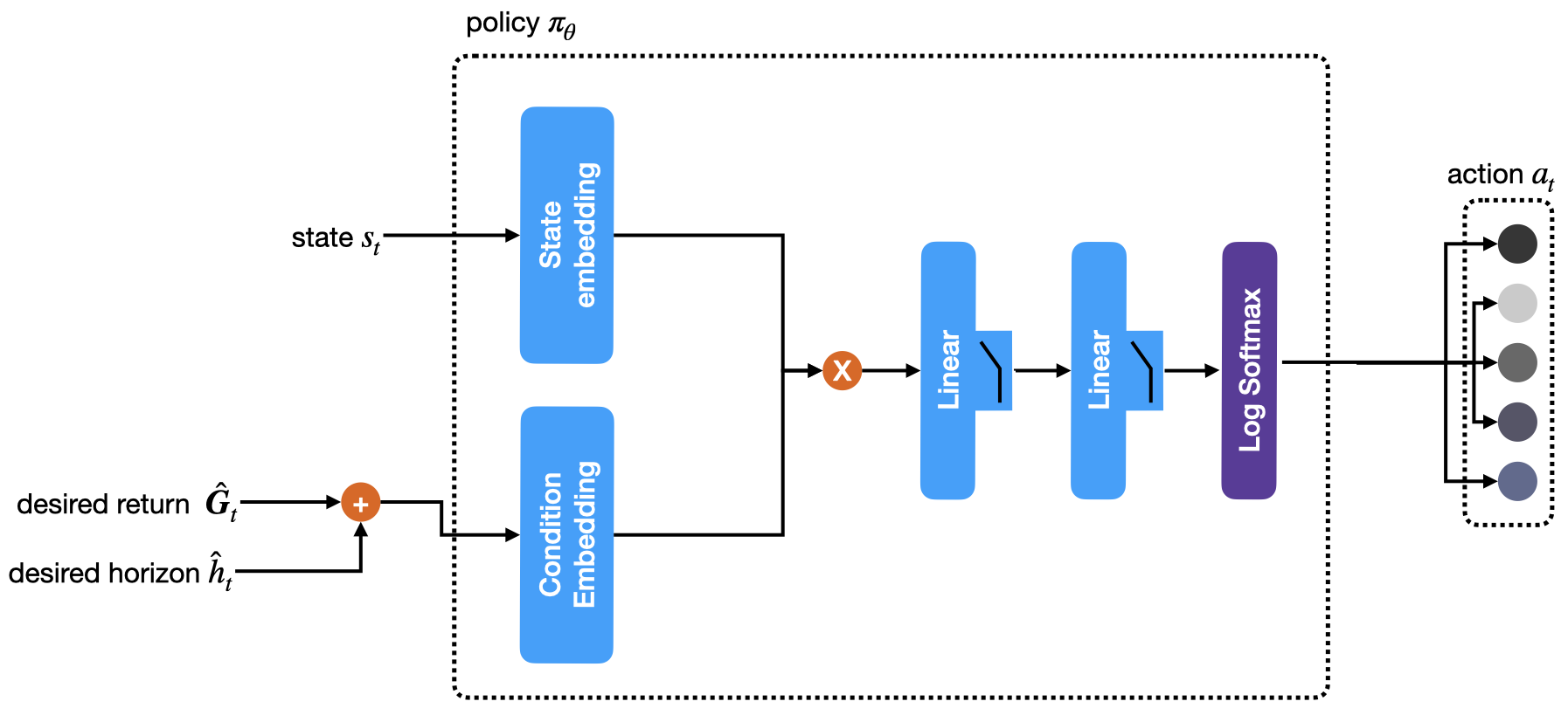
Just like PCN, LCN uses a single neural network to learn policy , which maps the current state , the desired horizon and the desired return to the next action . Note that is a vector, with equal to the number of objectives. The network receives an input tuple and returns a probability distribution over the next actions. It is trained with supervised learning on samples collected by the agent during exploration. The network updates its parameters using a cross-entropy loss function:
| (6) |
where is the batch size, is the -th sample action taken by the agent (ground truth), if and otherwise and represents the predicted probability of action for the -th sample, conditioned on its specific state , horizon , and return .
The training process involves sampling collected, non-dominated experiences, and then training the policy with supervised learning to imitate these experiences. Given a sufficient number of good experiences, the agent will learn good policies.
5.2 Collecting experiences
LCN is an off-policy method that learns the policy network by interacting with the environment, collecting experiences, and storing them in an Experience Replay (ER) buffer. These experiences are then used to train the policy via supervised learning (?, ?). Because action selection involves conditioning the network on a specified return, the primary mechanism for collecting higher-quality experiences is to iteratively improve the desired return used as the conditioning input.
To achieve this improvement, a non-dominated return is randomly sampled from the current non-dominated experiences in the ER buffer. This sampled return is then increased by a value drawn from a uniform distribution , where represents the standard deviation of all non-dominated points in the ER buffer (?). The updated return is subsequently used as the input for the policy network. Through this iterative process—refining the condition, collecting improved experiences, and training the policy network on non-dominated experiences—the network progressively learns to approximate all non-dominated trade-offs, forming a Lorenz coverage set. To ensure that the ER buffer contains experiences that will contribute most to performance improvement, however, the buffer must be filtered to retain only the most useful experiences.
5.3 Filtering experiences
PCN improves the experience replay buffer by filtering out experiences that are far away from the currently approximated Pareto front (non-dominated collected experiences). This is done by calculating the distance of each collected experience to the closest non-Pareto-dominated point in the buffer. In addition, a crowding distance is calculated for each point, measuring its distance to its closest neighbors (?). Points with many neighbors have a high crowding distance and are penalized by doubling their distance metric, ensuring that ER experiences are distributed throughout the objective space (?). With this approach, the set of Pareto-optimal solutions grows exponentially with the number of states and objectives, and maintaining a good ER buffer becomes a great challenge. In applications where fairness is important, much of the Pareto front is undesirable.
Lorenz Conditioned Networks (LCN), on the other hand, seek fairly distributed policies. Thus, the evaluation of each experience in the Experience Replay buffer is determined by its proximity to the nearest non-Lorenz dominated point . In Figure 2 (left) we show an example of this distance calculation. We denote the distance between an experience and a reference point as , where is the nearest non-Lorenz-dominated point, which we refer to as reference point. We formalize the final distance for the evaluation as follows:
| (7) |
Where is the crowding distance of and is the crowding distance threshold. A constant penalty is added to the points below the threshold, whose distance is also doubled. The points in the ER buffer are sorted based on, and those with the highest get replaced first when a better experience is collected.
5.4 Improving the filtering mechanism with reference points
The nearest-point filtering method employed by previous works has two drawbacks. Firstly, during exploration, stored experiences undergo significant changes as the agent discovers new, improved trajectories. This leads to a volatile ER buffer and moving targets, posing stability challenges during supervised learning. Secondly, we know in advance that certain experiences, even if non-dominated, are undesirable due to their unfair distribution of rewards.
Consider, for example, vectors: and their corresponding Lorenz vectors . Both and are non-Lorenz dominated, and would typically be used as targets for evaluating other experiences. However, is not a desirable target due to its unfair distribution of rewards (this is essentially a limitation of Lorenz dominance, when one objective is very large). To address these issues, we adopt the concept of reference points from Multi-Objective Optimization (?, ?, ?), and propose reference points for filtering the experiences. We introduce two reference point mechanisms: a redistribution mechanism and a mean reference point mechanism. Both of these reference points are optimistic, meaning that the agent seeks to minimize the distance to them.
5.4.1 Redistributed Reference Point (LCN-Redist)
This mechanism draws inspiration from the Pigou-Dalton principle we introduced in Section 3.2. Under this axiomatic principle, any experience in the ER buffer can be adjusted to provide a more desirable one. We identify the experience with the highest sum of rewards and evenly distribute the total reward across all dimensions of the vector. This is then assigned as the new reference point for all experiences :
| (8) |
5.4.2 Non-Dominated Mean Reference Point (LCN-Mean)
Additionally, we propose an alternative, simpler reference point mechanism: a straightforward averaging of all non-Lorenz dominated vectors in the experience replay (ER) buffer. This approach provides a non-intrusive method for incorporating collected experiences, while simultaneously smoothing out outlier non-dominated points. The reference point, denoted as , is defined as follows: Let represent the set of non-Lorenz dominated experiences in the ER buffer,
| (9) |
In Figure 2 (left) we show how this approach defines a reference point.
6 A Large Scale Many-Objective Environment
Existing discrete MORL benchmarks are often small-scale, with small state-action spaces or low-dimensional objective spaces (?, ?). In addition, they do not cover allocation of resources such as public transport, where fairness in the distribution is crucial. We introduce a novel and modular MORL environment, named the Multi-Objective Transport Network Design Problem (MO-TNDP). Built on MO-Gymnasium (?), the MO-TNDP environment simulates public transport design in cities of varying size and morphology, addressing TNDP, an NP-hard optimization problem aiming to generate a transport line that maximizes the satisfied travel demand (?).
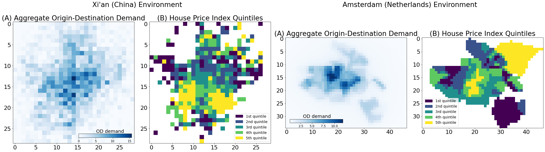
In MO-TNDP, a city is represented as , a grid with equally sized cells. The mobility demand forecast between cells is captured by an Origin-Destination (OD) flow matrix . Each cell is associated with a socioeconomic group , which determines the dimensionality of the reward function. In this paper, we scale it from 2 to 10 groups (objectives).
Episodes last a predefined number of steps. The agent traverses the city, connecting grid cells with eight available actions (movement in all directions). At each time step, the agent receives a vectorial reward of dimension , each corresponding to the percent satisfaction of the demand of each group. We formulate it as an MOMDP , where is the current location of the agent, is the next direction of movement, and is the additional demand satisfied by taking the last action for each group. Given the discrete and episodic nature, we set the discount factor to 1. The transition function is deterministic, and each episode starts in the same state.
Additional directional constraints can be imposed on the agent action space. The environment code enables developers to modify the city object, incorporating adjustments to grid size, OD matrix, cell group membership, and directional constraints, making it adaptable to any city. It supports both creating transport networks from scratch and expanding existing ones. MO-TNDP is available online 222Githup repository: https://github.com/dimichai/mo-tndp.
7 Experiments
We focus on two cities: Xi’an in China (841 cells, 20 episode steps) and Amsterdam in the Netherlands (1645 cells, 10 episode steps). Group membership for cells is determined by the average house price, which is divided into 2-10 equally sized buckets. Figure 3 illustrates two instances of the MO-TNDP environment for five objectives (a map of group membership for all objectives is provided in the supplementary material). LCN is built using the MORL-Baselines library and the code is attached as supplementary material (?).
Through a Bayesian hyperparameter search of 100 runs, we tuned the batch size, learning rate, ER buffer size, number of layers, and hidden dimension across all reported models, environments, and objective dimensions (details in the supplementary material). We compare LCN with two state-of-the-art multi-policy baselines: PCN (?) and GPI-LS (?), on widely used MO evaluation metrics. To fairly compare them, we trained all algorithms for a maximum of steps.
7.1 Evaluation Metrics
We use three common MO evaluation metrics to compare our method with the baselines. Hypervolume: an axiomatic metric that measures the volume of a set of points relative to a specific reference point and is maximized for the Pareto front. In general, it assesses the quality of a set of non-dominated solutions, its diversity, and spread (?).
| (10) |
where is the set of non-dominated policies, computes the Lebesgue measure of the input space and is the box spanned by the reference and policy value.
Expected Utility Metric (EUM): a utility-based metric that measures the expected utility of a given set of solutions, under some distribution of utility functions. EUM measures the actual expected utility of the policies, and is more interpretable compared to axiomatic approaches like the hypervolume (?). The score is defined as:
| (11) |
where is the set of non-dominated policies, is a distribution over utility functions (we use 100 equidistant weight vectors as was done in (?)) and is the value of the best policy in the , according to the utility function , defined by the sampled weights.
Sen Welfare: a welfare function, inspired by Sen’s social welfare theory, that combines total efficiency (total satisfied demand) and equality into a single measure. Equality is expressed through the Gini coefficient—a quantification of the Lorenz curve that measures reward distribution among groups (with indicating perfect equality and perfect inequality) (?). The final score is measured as follows:
| (12) |
where is the sum of the returns of all objectives in policy , and is its Gini Index. We use this metric for comparative purposes, reflecting a balanced scenario where both efficiency and equality are considered. Sen welfare has been utilized in economic simulations employing RL before (?). A higher Sen welfare value signifies increased efficiency and equity.
7.2 Results
In addition to the MO-TNDP environment, we also tested our methods on the DeepSeaTreasure environment, a common two-objective MORL benchmark where an agent controls a submarine and collects treasures (?). The agent faces a trade-off between fuel consumption and treasure value — moving uses fuel, but treasures at greater depths tend to be more valuable. Since the time objective is negative, only the baseline LCN is applicable in our experiments.
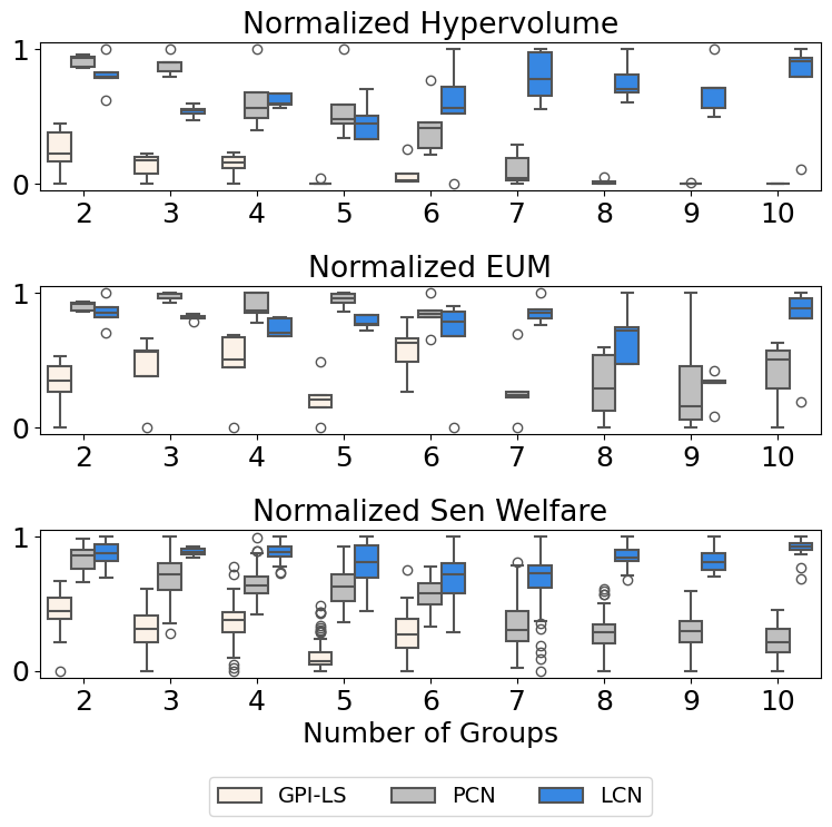
In Table 1, we show that LCN performs on par with PCN on the DeepSeaTreasure environment. In the rest of this section, we focus on MO-TNDP. The results discussed here are based on 5 different random seeded runs. Figure 4 (a) presents a comparison between PCN, GPI-LS and LCN across all objectives in the MO-TNDP-Xi’an environment, and Figure 4 (b) compares the vanilla LCN to the reference point alternatives.
| GPI-LS | PCN | LCN | |
|---|---|---|---|
| HV | |||
| EUM |
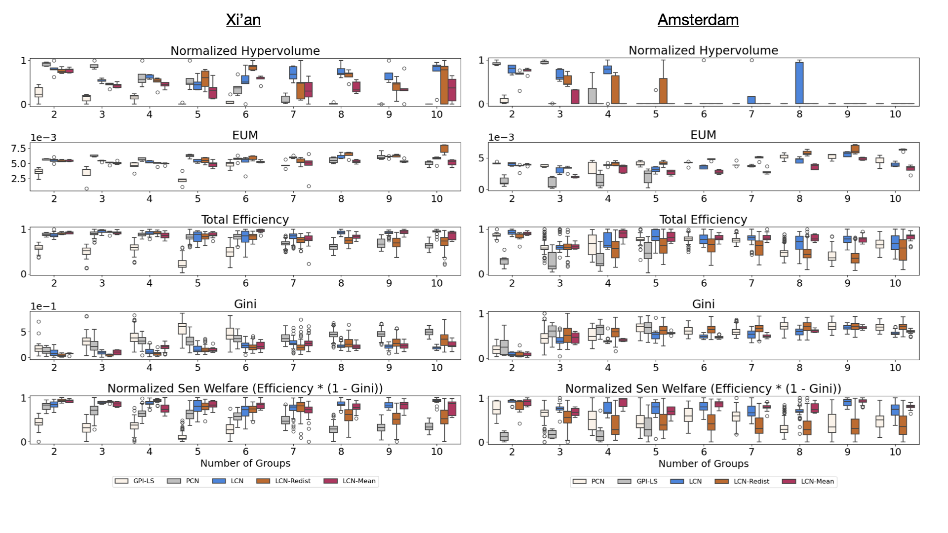
7.3 LCN outperforms PCN on many objective settings
As shown in Figure 4 (a), GPI-LS exhibits significantly lower performance across all objectives compared to PCN and LCN (GPI-LS was only tested up to objectives due to the exponentially increasing runtime). This performance gap is primarily due to the combination of the high-dimensional state-action-reward space and the limited number of timesteps. The original experiments on larger domains were conducted over more than k steps; to ensure a fair comparison, we have restricted training to k steps.
We focus on PCN vs LCN on the rest of the discussion. PCN shows strong performance on hypervolume and EUM in environments with 2–6 objectives. This is expected, as PCN is designed to learn diverse, non-Pareto-dominated solutions, which maximize these metrics. However, for larger objectives, LCN surpasses PCN even in hypervolume and EUM — metrics it is not specifically designed for. This occurs because, given the high state-action space of the environment, the non-Pareto-dominated solutions significantly expand with objectives, making the supervised training of PCN challenging. Furthermore, we observe that when scaling above seven objective, hypervolume for PCN collapses. In contrast, LCN effectively scales across the objective space, leveraging the smaller non-Lorenz-dominated set.
LCN consistently outperforms PCN in Sen welfare across all objectives. The Sen Welfare metric, which promotes solutions balancing efficiency and equality, shows that LCN excels in generating effective policies even when the solution space is constrained. In particular, LCN maintains its superior performance relative to PCN even as the number of objectives increases.
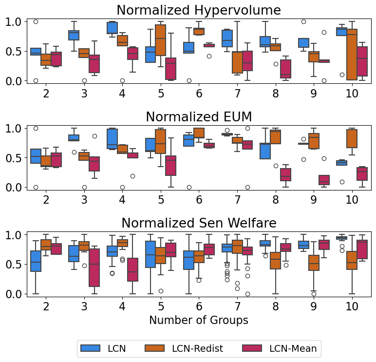
7.4 Reference points improve training
In Figure 4 (b), we compare the reference point mechanisms (LCN-Redist and LCN-Mean) with vanilla LCN. While the axiomatic hypervolume metric shows minimal impact of reference points on the model’s performance, the utility-based metrics, particularly EUM and Sen Welfare, reveal a different story. Vanilla LCN performs well when the objective space is limited. However, as the number of objectives increases, the introduction of reference points increases stability and outperforms the raw distance from non-dominated points.
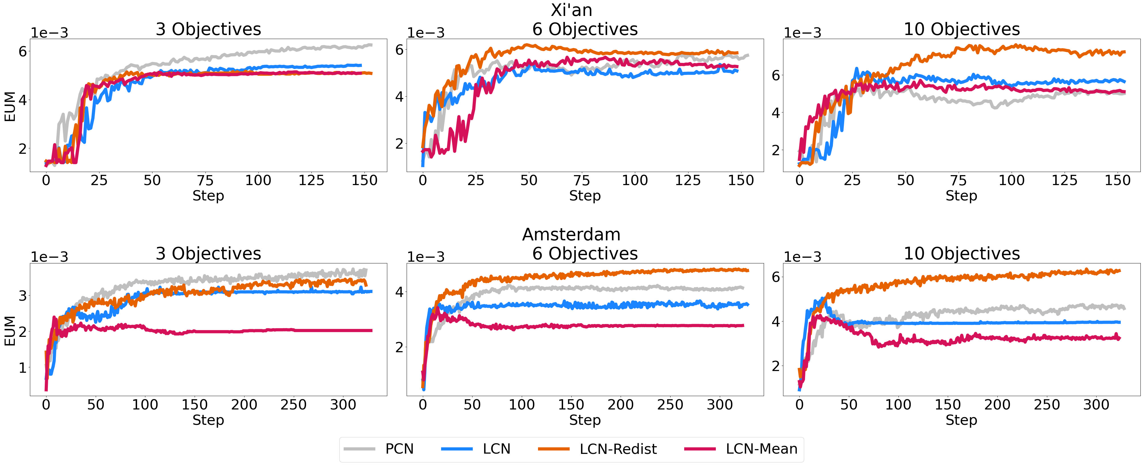
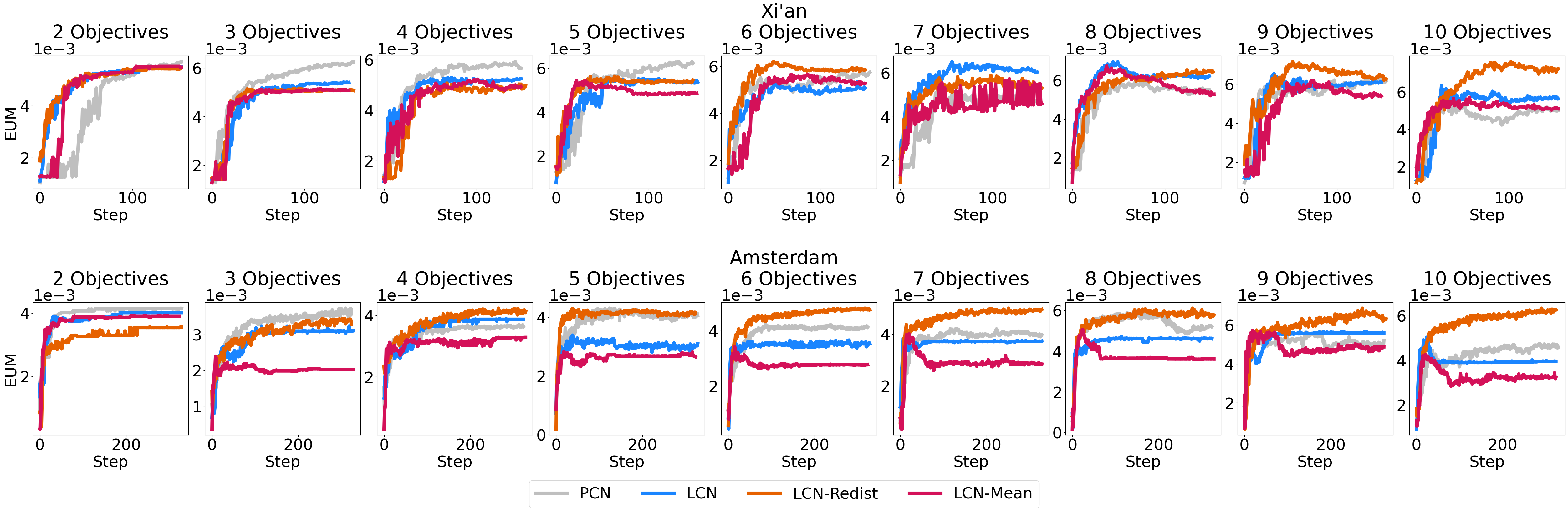
Specifically, LCN-Redist demonstrates superior performance in EUM when . Although this seems counterintuitive, the redistribution mechanism, which creates a reference point with equal objectives, also ensures that all objectives are represented, even if they were absent in the original vector. This approach promotes policies that offer desirable trade-offs across the solution spectrum. The effectiveness of LCN-Redist is further illustrated by the learning curves in Figure 5.
Conversely, LCN-Mean performs the worst in EUM as the number of objectives increases. This outcome can be attributed to the potential skewing of the mean vector by large disparities among dimensions. If a group is consistently underrepresented in the collected experiences, its mean dimension will be close to zero, negatively affecting EUM.
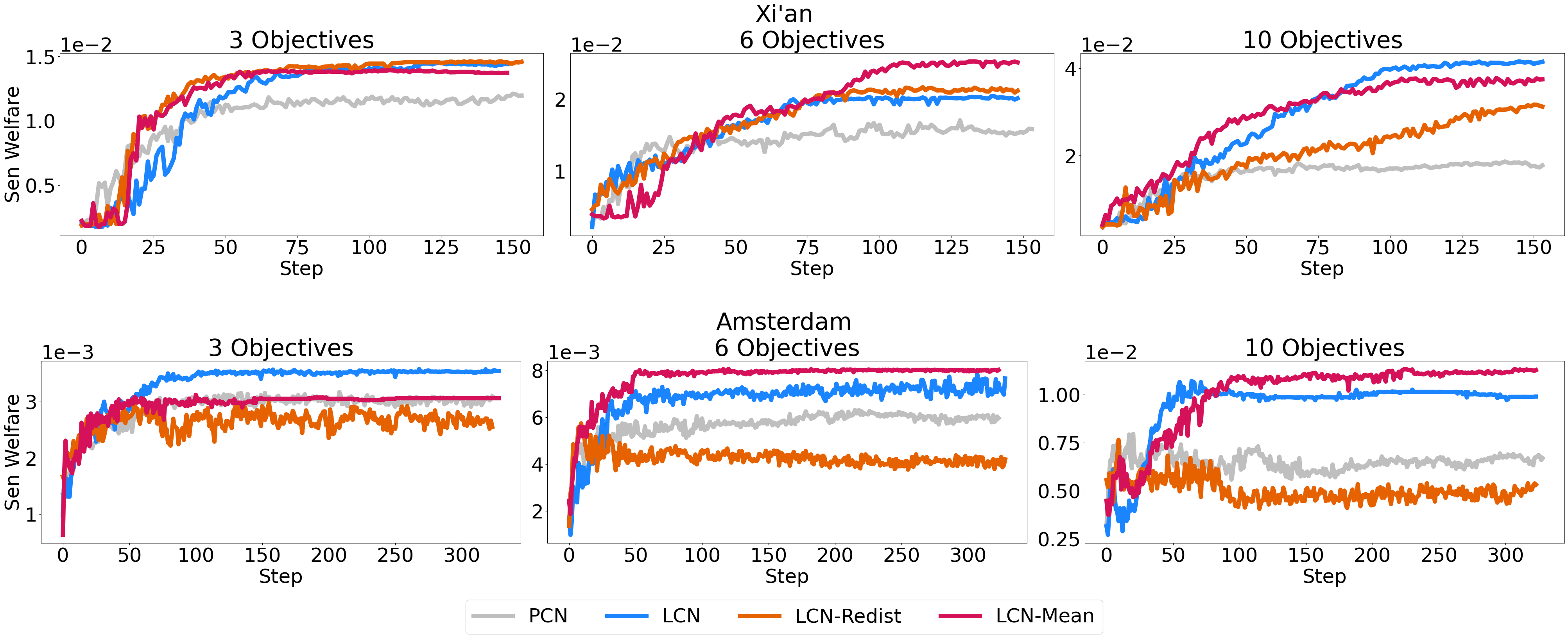
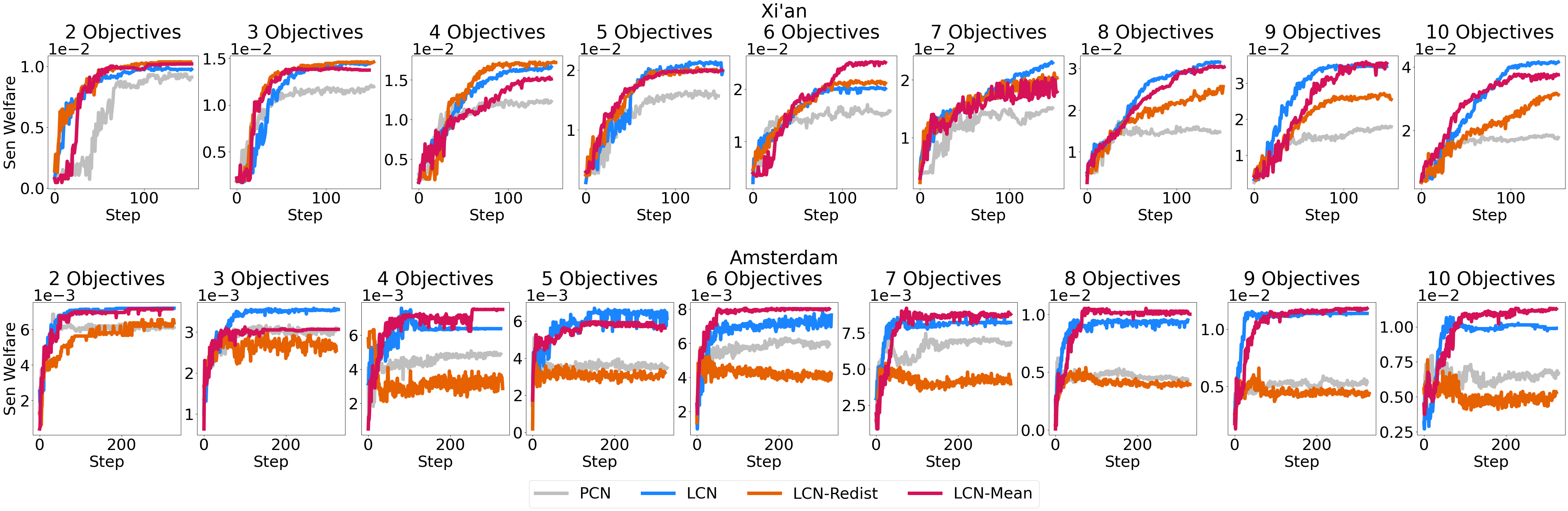
However, LCN-Mean performs great in Sen Welfare across all objectives, offering better stability than LCN-Redist. This result is expected, as LCN is designed to maximize Sen Welfare. LCN-Mean effectively balances outliers and creates reference points that balance efficiency and equality with minimal intervention. The learning curves for Sen Welfare are presented in Figure 6.
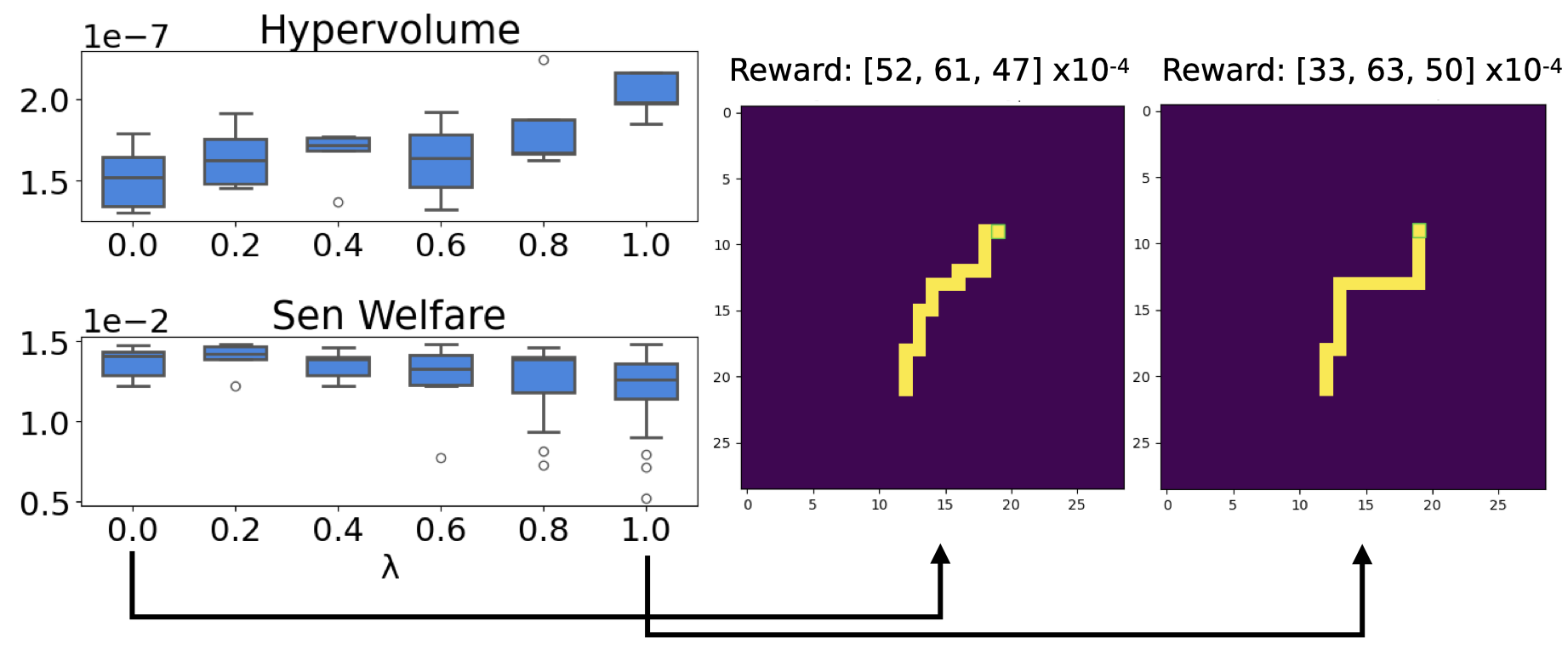
7.5 -LCN can be used to achieve control over the amount of fairness preference
In Figure 7, we illustrate the flexibility of -LCN in achieving diverse solutions across different fairness preferences. When , there is little flexibility, as the goal is to find the most equally distributed policies. This results in high performance for Sen Welfare but, as expected, lower performance in terms of hypervolume due to the concentrated solutions, which cover a smaller area. On the other hand, when , the space of accepted solutions expands, leading to a larger hypervolume. However, by accepting less fair solutions, the overall Sen Welfare decreases, adding an extra layer of complexity to the decision-making process. On the right side of the figure, we also show two transport lines originating from the same cell, one for and the other for . While the lines follow a similar direction, the placement of stations and the areas they traverse can differ substantially based on the fairness preference.
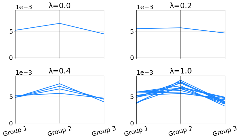
In Figure 8, we present parallel coordinate plots of the learned coverage sets for various values of . Here, too we demonstrate that as increases, the flexibility for distributing rewards less fairly among different groups also increases. This leads to an expanded coverage set, providing the decision maker with more policy trade-offs.
8 Conclusion
We addressed key challenges in multi-objective, multi-policy reinforcement learning, by proposing methods that perform well over large state-action and objective spaces. We developed a new, multi-objective environment for simulating Public Transport Network Design, thereby enhancing the applicability of MORL to real-world scenarios. We proposed LCN, an adaptation of state-of-the-art methods that outperforms baselines in high-reward dimensions. Finally, we present an effective method for controlling the fairness constraint. These contributions move the research field toward more realistic and applicable solutions in real-world contexts, thereby advancing the state-of-the-art in algorithmic fairness in sequential decision-making and MORL.
Acknowledgments
This research was in part supported by the European Union’s Horizon Europe research and innovation programme under grant agreement No 101120406 (PEER). DM is supported by the Innovation Center for AI (ICAI, The Netherlands). WR is supported by the Research Foundation – Flanders (FWO), grant number 1197622N. F. P. Santos acknowledges funding by the European Union (ERC, RE-LINK, 101116987).
References
- Abels, Roijers, Lenaerts, Nowé, and Steckelmacher Abels, A., Roijers, D., Lenaerts, T., Nowé, A., and Steckelmacher, D. (2019). Dynamic Weights in Multi-Objective Deep Reinforcement Learning. In Proceedings of the 36th International Conference on Machine Learning, pp. 11–20. PMLR. ISSN: 2640-3498.
- Adler Adler, M. D. (2013). The Pigou-Dalton Principle and the Structure of Distributive Justice..
- Alegre, Bazzan, Roijers, Nowé, and da Silva Alegre, L. N., Bazzan, A. L. C., Roijers, D. M., Nowé, A., and da Silva, B. C. (2023). Sample-efficient multi-objective learning via generalized policy improvement prioritization. In Proceedings of the 2023 International Conference on Autonomous Agents and Multiagent Systems, AAMAS ’23, p. 2003–2012, Richland, SC. International Foundation for Autonomous Agents and Multiagent Systems.
- Alegre, Felten, Talbi, Danoy, Nowé, Bazzan, and da Silva Alegre, L. N., Felten, F., Talbi, E.-G., Danoy, G., Nowé, A., Bazzan, A. L. C., and da Silva, B. C. (2022a). MO-Gym: A library of multi-objective reinforcement learning environments. In Proceedings of the 34th Benelux Conference on Artificial Intelligence BNAIC/Benelearn 2022.
- Alegre, Bazzan, and Silva Alegre, L. N., Bazzan, A., and Silva, B. C. D. (2022b). Optimistic Linear Support and Successor Features as a Basis for Optimal Policy Transfer. In Proceedings of the 39th International Conference on Machine Learning, pp. 394–413. PMLR. ISSN: 2640-3498.
- Basaklar, Gumussoy, and Ogras Basaklar, T., Gumussoy, S., and Ogras, U. Y. (2023). Pd-morl: Preference-driven multi-objective reinforcement learning algorithm..
- Blandin and Kash Blandin, J., and Kash, I. A. (2024). Group fairness in reinforcement learning via multi-objective rewards..
- Cao and Zhan Cao, Y., and Zhan, H. (2021). Efficient multi-objective reinforcement learning via multiple-gradient descent with iteratively discovered weight-vector sets. Journal of Artificial Intelligence Research, 70, 319–349.
- Chabane, Basseur, and Hao Chabane, B., Basseur, M., and Hao, J.-K. (2019). Lorenz dominance based algorithms to solve a practical multiobjective problem. Computers & Operations Research, 104, 1–14.
- Chen, Wang, and Lan Chen, J., Wang, Y., and Lan, T. (2021). Bringing Fairness to Actor-Critic Reinforcement Learning for Network Utility Optimization. In IEEE INFOCOM 2021 - IEEE Conference on Computer Communications, pp. 1–10. ISSN: 2641-9874.
- Chen, Wang, Thomas, and Ulmer Chen, X., Wang, T., Thomas, B. W., and Ulmer, M. W. (2023). Same-day delivery with fair customer service. European Journal of Operational Research, 308(2), 738–751.
- Cheng, Jin, Olhofer, and Sendhoff Cheng, R., Jin, Y., Olhofer, M., and Sendhoff, B. (2016). A reference vector guided evolutionary algorithm for many-objective optimization. IEEE Transactions on Evolutionary Computation, 20(5), 773–791.
- Cimpeana, Jonkerb, Libina, and Nowéa Cimpeana, A., Jonkerb, C., Libina, P., and Nowéa, A. (2023). A multi-objective framework for fair reinforcement learning. In Multi-Objective Decision Making Workshop 2023.
- Deb, Agrawal, Pratap, and Meyarivan Deb, K., Agrawal, S., Pratap, A., and Meyarivan, T. (2000). A Fast Elitist Non-dominated Sorting Genetic Algorithm for Multi-objective Optimization: NSGA-II. In Schoenauer, M., Deb, K., Rudolph, G., Yao, X., Lutton, E., Merelo, J. J., and Schwefel, H.-P. (Eds.), Parallel Problem Solving from Nature PPSN VI, Lecture Notes in Computer Science, pp. 849–858, Berlin, Heidelberg. Springer.
- Deb and Jain Deb, K., and Jain, H. (2014). An evolutionary many-objective optimization algorithm using reference-point-based nondominated sorting approach, part i: Solving problems with box constraints. IEEE Transactions on Evolutionary Computation, 18(4), 577–601.
- Delgrange, Reymond, Nowe, and Pérez Delgrange, F., Reymond, M., Nowe, A., and Pérez, G. (2023). Wae-pcn: Wasserstein-autoencoded pareto conditioned networks. In Cruz, F., Hayes , C., Wang, C., and Yates, C. (Eds.), Proc. of the Adaptive and Learning Agents Workshop (ALA 2023) (15 edition)., Vol. https://alaworkshop2023.github.io/, pp. 1–7. 2023 Adaptive and Learning Agents Workshop at AAMAS, ALA 2023 ; Conference date: 29-05-2023 Through 30-05-2023.
- Fan, Peng, Tian, and Fain Fan, Z., Peng, N., Tian, M., and Fain, B. (2023). Welfare and Fairness in Multi-objective Reinforcement Learning. In Proceedings of the 2023 International Conference on Autonomous Agents and Multiagent Systems, AAMAS ’23, pp. 1991–1999, Richland, SC. International Foundation for Autonomous Agents and Multiagent Systems.
- Farahani, Miandoabchi, Szeto, and Rashidi Farahani, R. Z., Miandoabchi, E., Szeto, W. Y., and Rashidi, H. (2013). A review of urban transportation network design problems. European journal of operational research, 229(2), 281–302.
- Fasihi, Tavakkoli-Moghaddam, and Jolai Fasihi, M., Tavakkoli-Moghaddam, R., and Jolai, F. (2023). A bi-objective re-entrant permutation flow shop scheduling problem: minimizing the makespan and maximum tardiness. Operational Research, 23(2), 29.
- Felten, Alegre, Nowé, Bazzan, Talbi, Danoy, and Silva Felten, F., Alegre, L. N., Nowé, A., Bazzan, A. L. C., Talbi, E. G., Danoy, G., and Silva, B. C. d. (2023). A toolkit for reliable benchmarking and research in multi-objective reinforcement learning. In Proceedings of the 37th Conference on Neural Information Processing Systems (NeurIPS 2023).
- Felten, Talbi, and Danoy Felten, F., Talbi, E.-G., and Danoy, G. (2024). Multi-objective reinforcement learning based on decomposition: A taxonomy and framework. J. Artif. Int. Res., 79.
- Feng and Zhang Feng, T., and Zhang, J. (2014). Multicriteria evaluation on accessibility-based transportation equity in road network design problem. Journal of Advanced Transportation, 48(6), 526–541. _eprint: https://onlinelibrary.wiley.com/doi/pdf/10.1002/atr.1202.
- Gajane, Saxena, Tavakol, Fletcher, and Pechenizkiy Gajane, P., Saxena, A., Tavakol, M., Fletcher, G., and Pechenizkiy, M. (2022). Survey on Fair Reinforcement Learning: Theory and Practice.. arXiv:2205.10032 [cs].
- Hayes, Rădulescu, Bargiacchi, Källström, Macfarlane, Reymond, Verstraeten, Zintgraf, Dazeley, Heintz, Howley, Irissappane, Mannion, Nowé, Ramos, Restelli, Vamplew, and Roijers Hayes, C. F., Rădulescu, R., Bargiacchi, E., Källström, J., Macfarlane, M., Reymond, M., Verstraeten, T., Zintgraf, L. M., Dazeley, R., Heintz, F., Howley, E., Irissappane, A. A., Mannion, P., Nowé, A., Ramos, G., Restelli, M., Vamplew, P., and Roijers, D. M. (2022). A practical guide to multi-objective reinforcement learning and planning. Autonomous Agents and Multi-Agent Systems, 36(1), 26.
- Hu, Zhang, Xia, Wei, Dai, and Li Hu, X., Zhang, Y., Xia, H., Wei, W., Dai, Q., and Li, J. (2023). Towards fair power grid control: A hierarchical multi-objective reinforcement learning approach. IEEE Internet of Things Journal, PP, 1–1.
- Jabbari, Joseph, Kearns, Morgenstern, and Roth Jabbari, S., Joseph, M., Kearns, M., Morgenstern, J., and Roth, A. (2017). Fairness in reinforcement learning. In Precup, D., and Teh, Y. W. (Eds.), Proceedings of the 34th International Conference on Machine Learning, Vol. 70 of Proceedings of Machine Learning Research, pp. 1617–1626. PMLR.
- Ju, Ghosh, and Shroff Ju, P., Ghosh, A., and Shroff, N. B. (2023). Achieving fairness in multi-agent markov decision processes using reinforcement learning..
- Kumar and Yeoh Kumar, A., and Yeoh, W. (2023). Fairness in scarce societal resource allocation: A case study in homelessness applications. In Proceedings of the workshop” Autonomous Agents for Social Good”. online.
- Kumar, Peng, and Levine Kumar, A., Peng, X. B., and Levine, S. (2019). Reward-conditioned policies..
- Lopez, Behrisch, Bieker-Walz, Erdmann, Flötteröd, Hilbrich, Lücken, Rummel, Wagner, and Wiessner Lopez, P. A., Behrisch, M., Bieker-Walz, L., Erdmann, J., Flötteröd, Y.-P., Hilbrich, R., Lücken, L., Rummel, J., Wagner, P., and Wiessner, E. (2018). Microscopic Traffic Simulation using SUMO. In 2018 21st International Conference on Intelligent Transportation Systems (ITSC), pp. 2575–2582. ISSN: 2153-0017.
- Mandal and Gan Mandal, D., and Gan, J. (2023). Socially Fair Reinforcement Learning.. arXiv:2208.12584 [cs].
- Mannion, Heintz, Karimpanal, and Vamplew Mannion, P., Heintz, F., Karimpanal, T. G., and Vamplew, P. (2021). Multi-objective decision making for trustworthy ai. In Proceedings of the Multi-Objective Decision Making (MODeM) Workshop.
- Moffaert and Nowé Moffaert, K. V., and Nowé, A. (2014). Multi-Objective Reinforcement Learning using Sets of Pareto Dominating Policies. Journal of Machine Learning Research, 15(107), 3663–3692.
- Nguyen, Nguyen, Vamplew, Nahavandi, Dazeley, and Lim Nguyen, T. T., Nguyen, N. D., Vamplew, P., Nahavandi, S., Dazeley, R., and Lim, C. P. (2020). A multi-objective deep reinforcement learning framework. Engineering Applications of Artificial Intelligence, 96, 103915.
- Osika, Salazar, Roijers, Oliehoek, and Murukannaiah Osika, Z., Salazar, J. Z., Roijers, D. M., Oliehoek, F. A., and Murukannaiah, P. K. (2023). What lies beyond the pareto front? A survey on decision-support methods for multi-objective optimization. In Proceedings of the Thirty-Second International Joint Conference on Artificial Intelligence, IJCAI 2023, 19th-25th August 2023, Macao, SAR, China, pp. 6741–6749. ijcai.org.
- Parisi, Pirotta, and Restelli Parisi, S., Pirotta, M., and Restelli, M. (2016). Multi-objective reinforcement learning through continuous pareto manifold approximation. Journal of Artificial Intelligence Research, 57, 187–227.
- Perny, Weng, Goldsmith, and Hanna Perny, P., Weng, P., Goldsmith, J., and Hanna, J. (2013). Approximation of Lorenz-Optimal Solutions in Multiobjective Markov Decision Processes.. arXiv:1309.6856 [cs].
- Peschl, Zgonnikov, Oliehoek, and Siebert Peschl, M., Zgonnikov, A., Oliehoek, F. A., and Siebert, L. C. (2021). MORAL: Aligning AI with Human Norms through Multi-Objective Reinforced Active Learning.. arXiv:2201.00012 [cs].
- Rădulescu, Mannion, Roijers, and Nowé Rădulescu, R., Mannion, P., Roijers, D. M., and Nowé, A. (2019). Equilibria in multi-objective games: a utility-based perspective. In Proceedings of the adaptive and learning agents workshop (ALA-19) at AAMAS.
- Reymond, Bargiacchi, and Nowé Reymond, M., Bargiacchi, E., and Nowé, A. (2022a). Pareto conditioned networks. In Proceedings of the 21st International Conference on Autonomous Agents and Multiagent Systems, AAMAS ’22, p. 1110–1118, Richland, SC. International Foundation for Autonomous Agents and Multiagent Systems.
- Reymond, Hayes, Willem, Rădulescu, Abrams, Roijers, Howley, Mannion, Hens, Nowé, and Libin Reymond, M., Hayes, C. F., Willem, L., Rădulescu, R., Abrams, S., Roijers, D. M., Howley, E., Mannion, P., Hens, N., Nowé, A., and Libin, P. (2022b). Exploring the Pareto front of multi-objective COVID-19 mitigation policies using reinforcement learning.. arXiv:2204.05027 [cs, q-bio].
- Rodriguez-Soto, Lopez-Sanchez, and Aguilar Rodriguez-Soto, M., Lopez-Sanchez, M., and Aguilar, J. A. R. (2021). Multi-Objective Reinforcement Learning for Designing Ethical Environments.. Vol. 1, pp. 545–551. ISSN: 1045-0823.
- Rodriguez-Soto, Serramia, Lopez-Sanchez, and Rodriguez-Aguilar Rodriguez-Soto, M., Serramia, M., Lopez-Sanchez, M., and Rodriguez-Aguilar, J. A. (2022). Instilling moral value alignment by means of multi-objective reinforcement learning. Ethics and Information Technology, 24(1), 9.
- Roijers, Whiteson, and Oliehoek Roijers, D. M., Whiteson, S., and Oliehoek, F. A. (2015). Computing Convex Coverage Sets for Faster Multi-objective Coordination. Journal of Artificial Intelligence Research, 52, 399–443.
- Röpke Röpke, W. (2023). Reinforcement learning in multi-objective multi-agent systems. In Proceedings of the 2023 International Conference on Autonomous Agents and Multiagent Systems, AAMAS ’23, p. 2999–3001, Richland, SC. International Foundation for Autonomous Agents and Multiagent Systems.
- Ruiz-Montiel, Mandow, and Pérez-de-la Cruz Ruiz-Montiel, M., Mandow, L., and Pérez-de-la Cruz, J.-L. (2017). A temporal difference method for multi-objective reinforcement learning. Neurocomputing, 263, 15–25.
- Röpke, Reymond, Mannion, Roijers, Nowé, and Rădulescu Röpke, W., Reymond, M., Mannion, P., Roijers, D. M., Nowé, A., and Rădulescu, R. (2024). Divide and conquer: Provably unveiling the pareto front with multi-objective reinforcement learning..
- Satija, Lazaric, Pirotta, and Pineau Satija, H., Lazaric, A., Pirotta, M., and Pineau, J. (2023). Group fairness in reinforcement learning. Trans. Mach. Learn. Res., 2023.
- Schläpfer, Dong, O’Keeffe, Santi, Szell, Salat, Anklesaria, Vazifeh, Ratti, and West Schläpfer, M., Dong, L., O’Keeffe, K., Santi, P., Szell, M., Salat, H., Anklesaria, S., Vazifeh, M., Ratti, C., and West, G. B. (2021). The universal visitation law of human mobility. Nature, 593(7860), 522–527. Number: 7860 Publisher: Nature Publishing Group.
- Sen Sen, A. (1976). Poverty: An Ordinal Approach to Measurement. Econometrica, 44(2), 219–231. Publisher: [Wiley, Econometric Society].
- Shorrocks Shorrocks, A. F. (1983). Ranking income distributions. Economica, 50(197), 3–17.
- Siddique, Weng, and Zimmer Siddique, U., Weng, P., and Zimmer, M. (2020). Learning fair policies in multi-objective (Deep) reinforcement learning with average and discounted rewards. In III, H. D., and Singh, A. (Eds.), Proceedings of the 37th International Conference on Machine Learning, Vol. 119 of Proceedings of Machine Learning Research, pp. 8905–8915. PMLR.
- Vamplew, Dazeley, Berry, Issabekov, and Dekker Vamplew, P., Dazeley, R., Berry, A., Issabekov, R., and Dekker, E. (2011). Empirical evaluation methods for multiobjective reinforcement learning algorithms. Machine Learning, 84(1), 51–80.
- Vamplew, Smith, Källström, Ramos, Rădulescu, Roijers, Hayes, Heintz, Mannion, Libin, Dazeley, and Foale Vamplew, P., Smith, B. J., Källström, J., Ramos, G., Rădulescu, R., Roijers, D. M., Hayes, C. F., Heintz, F., Mannion, P., Libin, P. J. K., Dazeley, R., and Foale, C. (2022). Scalar reward is not enough: a response to Silver, Singh, Precup and Sutton (2021). Autonomous Agents and Multi-Agent Systems, 36(2), 41.
- Wang, Liu, Zhang, Feng, Huang, Li, and Zhang Wang, H.-n., Liu, N., Zhang, Y.-y., Feng, D.-w., Huang, F., Li, D.-s., and Zhang, Y.-m. (2020). Deep reinforcement learning: a survey. Frontiers of Information Technology & Electronic Engineering, 21(12), 1726–1744.
- Wei, Mao, Zhao, Zou, and An Wei, Y., Mao, M., Zhao, X., Zou, J., and An, P. (2020). City Metro Network Expansion with Reinforcement Learning. In Proceedings of the 26th ACM SIGKDD International Conference on Knowledge Discovery & Data Mining, pp. 2646–2656, Virtual Event CA USA. ACM.
- Yu, Qin, Lee, and Gao Yu, E. Y., Qin, Z., Lee, M. K., and Gao, S. (2022). Policy Optimization with Advantage Regularization for Long-Term Fairness in Decision Systems.. arXiv:2210.12546 [cs].
- Zheng, Trott, Srinivasa, Parkes, and Socher Zheng, S., Trott, A., Srinivasa, S., Parkes, D. C., and Socher, R. (2022). The AI Economist: Taxation policy design via two-level deep multiagent reinforcement learning. Science Advances, 8(18), eabk2607. Publisher: American Association for the Advancement of Science.
- Zimmer, Glanois, Siddique, and Weng Zimmer, M., Glanois, C., Siddique, U., and Weng, P. (2021). Learning Fair Policies in Decentralized Cooperative Multi-Agent Reinforcement Learning. In Proceedings of the 38th International Conference on Machine Learning, pp. 12967–12978. PMLR. ISSN: 2640-3498.
A Theoretical Results
In this section, we provide the detailed theoretical results for -LCN that we sketched on the main paper. In particular, we show that -Lorenz dominance is a generalisation of Lorenz dominance that can be used to flexibly set a desired fairness level. Moreover, by decreasing , the resulting solution set moves monotonically closer to the Lorenz front.
We first introduce a necessary auxiliary result in lemma 2 which shows that -Lorenz dominance implies Lorenz dominance.
Lemma 2.
and ,
| (13) |
Proof.
By contradiction, assume there is some and such that but does not Lorenz dominate . Then there is some smallest index such that . Since and , we know that . Then for all indices we have . Given that , we have that . However, this implies that and therefore does not -Lorenz dominate leading to a contradiction. ∎
In theorem 3 we use lemma 2 to demonstrate that when some vector -Lorenz dominates, it necessarily also dominates it for any smaller .
Theorem 3.
and ,
| (14) |
Proof.
Let . From Definition 3, this can equivalently be written as . In addition, from lemma 2 we know that since . Then, for any index we have that,
| (15) | ||||
| (16) | ||||
| (17) | ||||
| (18) |
where the last step holds since and by lemma 2. ∎
We now contribute an additional auxiliary result which guarantees that when some vector Pareto dominates another, it also -Lorenz dominates the vector. This result is an extension of the fact that Pareto dominance implies Lorenz dominance.
Lemma 4.
and ,
| (19) |
Proof.
From Definition 3, -Lorenz dominance can be written as . Let us first recall that (?). It is then necessary to demonstrate an analogous result for . We prove this by induction.
Let and . By contradiction, assume that but does not Pareto dominate . This implies that there is some index such that . Let us consider the four cases for and .
If and this cannot occur. Moreover, if both vectors are in reverse it also cannot be the case.
When and , cannot be greater than since by transitivy then also which is a contradiction. Furthermore, cannot be greater than because then which is again a contradiction.
The final case where and , gives the same contradictions.
Assuming that the result holds for vectors of dimension , we demonstrate that it must also hold for . Let and . Consider now and which are extensions of the vectors and . Then . By contradiction, assume again that does not dominate . Let be the smallest index where . There are four cases where this may occur. Either this happens when and have both not been inserted yet, has been inserted but not , has been inserted but not and both have been inserted. Clearly, when neither or both were inserted, this leads to a contradiction.
If only was inserted, by transitivity we have that and therefore which is a contradiction. Lastly, if only was inserted then and implying that and leading to a contradiction. ∎
Finally, we provide a proof for Theorem 1 of the main paper. This result demonstrates that when is , the solution set starts closest to the Pareto front and decreasing to monotonically reduces the solution set until it results in the Lorenz front. As such, by selecting a , a decision-maker can determine their preferred balance between Pareto optimality and Lorenz fairness. We first restate the theorem below and subsequently provide the proof.
Theorem 5.
(Referred to as Theorem 1 in the main text) and the following relations hold.
| (20) |
B Preparing the Xi’an and Amsterdam Environments.
The MO-TNDP environment released with this paper is adaptable for training an agent in any city, provided there are three elements: grid size (defined by the number of rows and columns), OD matrix, and group membership assigned to each grid cell. The grid size is specified as an argument in the constructor of the environment object, along with the file paths leading to the CSV files containing the OD matrix and group membership data. We have configured the environments for both Xi’an and Amsterdam, and these are included alongside the code for the environment.
Xi’an environment preparation
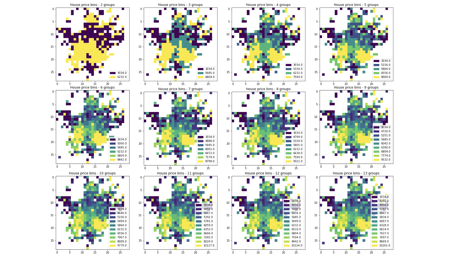
We generated the Xi’an environment utilizing the data provided by ?. 333source: https://github.com/weiyu123112/City-Metro-Network-Expansion-with-RL. The city is divided into a grid of dimensions , with cells of equal size (). The OD demand matrix was formulated using GPS data gathered from 25 million mobile phones, with their movements tracked over a one-month period Additionally, each cell is assigned an average house price index, which is categorized into quintiles. Figure 9 provides a comprehensive breakdown of the city into various sized groups.
Amsterdam environment preparation
We generate and release the data associated with the Amsterdam environment. The city is divided into a grid of dimensions , consisting of equally sizes cells of . The choice of this cell size takes into consideration Amsterdam’s smaller size compared to Xi’an. Since GPS data is unavailable for Amsterdam, we estimate the OD demand using the recently published universal law of human mobility, which states that the total mobility flow between two areas, denoted as and , depends on their distance and visitation frequency (?). The estimation is computed using the formula:
| (21) |
Where represents the total area of the origin location , is the (Manhattan) distance between and is the magnitude of flows, calculated as follows:
| (22) |
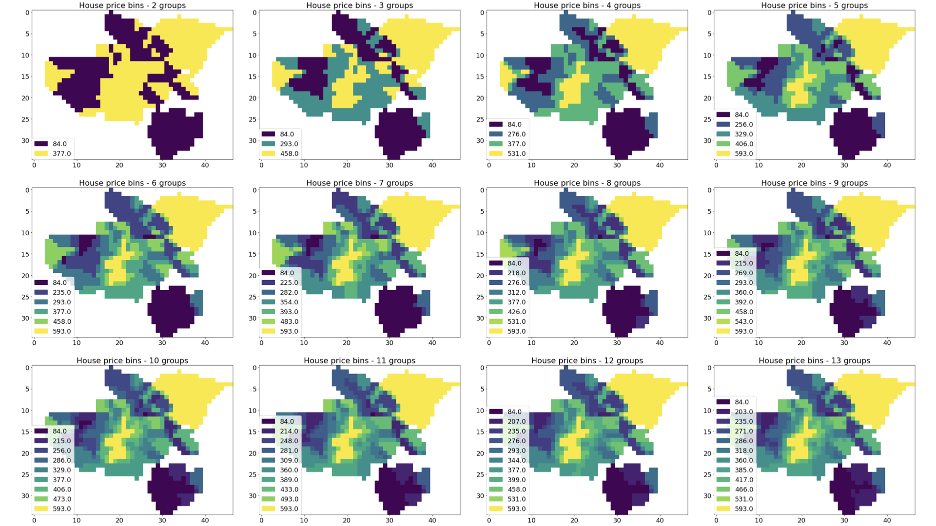
Where is the radius of area j. The flows are estimated for a full week, and in the model, this is accomplished by setting and to and respectively. Since the grid cells are of equal size in our case, the term can be omitted from the calculation. An illustration of the Amsterdam environment is presented in A detailed breakdown of the city into different-sized groups is depicted in Figure 10. Similar to the Xi’an environment, each cell in Amsterdam is associated with an average house price, sourced from the publicly available statistical bureau of The Netherlands dataset 444source: https://www.cbs.nl/nl-nl/maatwerk/2019/31/kerncijfers-wijken-en-buurten-2019.
C Experiment Reproducibility Details
Each model presented in the paper for training MO-TNDP was trained for 30000 steps. Hyperparameter were tuned via a bayes search over 100 settings, with the following ranges:
PCN/LCN
-
•
Batch size: [128, 256]
-
•
Learning Rate: [0.1, 0.01]
-
•
Number of Linear Layers: [1, 2]
-
•
Hidden Dims: [64, 128]
-
•
Experience Replay Buffer Size: [50, 100]
-
•
Model Updates: [5, 10]
GPI-LS
-
•
Network Architecture: [64, 64, 64]
-
•
Learning Rate: [0.00001, 0.0001, 0.001, 0.01]
-
•
Batch Size: [16, 32, 64, 128, 256, 512]
-
•
Buffer Size: [256, 512, 2048, 4096, 8192, 16384, 32768]
-
•
Learning Starts: 50
-
•
Target Net Update Frequency: [10, 20, 50, 100]
-
•
Gradient Updates: [1, 2, 5]
fig. 11 shows the architecture used for the policy network. In the provided code, we provide the exact commands to reproduce all of our experiments, including the environments, hyperparameters, and seeds used to generate our results. Furthermore, the details of the hyperparameters we used for each experiment are available on a public Notion page 555https://aware-night-ab1.notion.site/Project-B-MO-LCN-Experiment-Tracker-b4d21ab160eb458a9cff9ab9314606a7. Finally, we commit to sharing the output model weights upon request.
D
Additional Results
Total efficiency: measures how effectively a generated line captures the total travel demand of a city. It is calculated as the simple sum of all elements in the value vector – the sum of all satisfied demands for each group.
Gini coefficient: quantifies the reward distribution among various groups in the city. A value of 0 indicates perfect equality (equal percentage of satisfied OD flows per group), while 1 represents perfect inequality (only the demand of one group is satisfied). Although traditionally used to assess income inequality (?), it has also been employed in the context of transportation network design (?). In fig. 12 and table 2, we show detailed results on both Xi’an and Amsterdam for all objectives. fig. 13 and fig. 14 shows the learning curves of PCN and LCN for all objectives.
| Normalized Hypervolume | |||||||||
| Number of Objectives | |||||||||
| Xi’an | 2 | 3 | 4 | 5 | 6 | 7 | 8 | 9 | 10 |
| GPI-LS | |||||||||
| PCN | |||||||||
| LCN | |||||||||
| LCN-Redist. | |||||||||
| LCN-Mean | |||||||||
| Amsterdam | 2 | 3 | 4 | 5 | 6 | 7 | 8 | 9 | 10 |
| GPI-LS | |||||||||
| PCN | |||||||||
| LCN | |||||||||
| LCN-Redist. | |||||||||
| LCN-Mean | |||||||||
| Normalized EUM | |||||||||
| Xi’an | 2 | 3 | 4 | 5 | 6 | 7 | 8 | 9 | 10 |
| GPI-LS | |||||||||
| PCN | |||||||||
| LCN | |||||||||
| LCN-Redist. | |||||||||
| LCN-Mean | |||||||||
| Amsterdam | 2 | 3 | 4 | 5 | 6 | 7 | 8 | 9 | 10 |
| GPI-LS | |||||||||
| PCN | |||||||||
| LCN | |||||||||
| LCN-Redist. | |||||||||
| LCN-Mean | |||||||||
| Normalized Total Efficiency | |||||||||
| Xi’an | 2 | 3 | 4 | 5 | 6 | 7 | 8 | 9 | 10 |
| GPI-LS | |||||||||
| PCN | |||||||||
| LCN | |||||||||
| LCN-Redist. | |||||||||
| LCN-Mean | |||||||||
| Amsterdam | 2 | 3 | 4 | 5 | 6 | 7 | 8 | 9 | 10 |
| GPI-LS | |||||||||
| PCN | |||||||||
| LCN | |||||||||
| LCN-Redist. | |||||||||
| LCN-Mean | |||||||||
| Gini Index (the lower the better) | |||||||||
| Xi’an | 2 | 3 | 4 | 5 | 6 | 7 | 8 | 9 | 10 |
| GPI-LS | |||||||||
| PCN | |||||||||
| LCN | |||||||||
| LCN-Redist. | |||||||||
| LCN-Mean | |||||||||
| Amsterdam | 2 | 3 | 4 | 5 | 6 | 7 | 8 | 9 | 10 |
| GPI-LS | |||||||||
| PCN | |||||||||
| LCN | |||||||||
| LCN-Redist. | |||||||||
| LCN-Mean | |||||||||