mumax⁺: extensible GPU-accelerated micromagnetics and beyond

Abstract

We present the design and verification of mumax⁺, an extensible GPU-accelerated micromagnetic simulator with a Python user interface. It is a general solver for the space- and time-dependent evolution of the magnetization and related vector quantities, using a finite-difference discretization. In this work, we test the new features of mumax⁺, which are antiferromagnetism and elasticity, against several theoretical models including a dispersion relation for (elastic) antiferromagnets.

1 Introduction

In the last decades, micromagnetic calculations have been an essential tool in the development of the field of modern magnetism. Especially, the availability of open source[1, 2, 3, 4, 5] and GPU accelerated software packages [6, 7, 5, 8] have boosted the research, enabling the efficient numerical study of nano- and micrometer sized magnetic system efficiently, complementary to experimental studies.

In recent years, the research efforts shifted to more complex magnetic systems such as antiferromagnets and 2D magnetic heterostructures (Van der Waals systems).

mumax⁺ is a new and versatile GPU-accelerated micromagnetic simulation package. It calculates the space- and time-evolution of nano- to microscale magnets using a finite-difference scheme which has been independently designed from its predecessors mumaxn¹, mumax² and mumax³ [2, 3, 5]. Unlike its predecessors, it has a Python [9] based user interface. This allows users to use packages such as Numpy [10] and Scipy [11] to process their data directly. The Python module wraps the main part of the program, which is written in C++ [12] and CUDA [13]. The latter allows calculations to be done by a GPU, reducing computation time compared to CPU based programs. The use of CUDA requires the user to have an NVIDIA GPU in order to be able to compile mumax⁺. Another feature is that it’s possible to compile the package using double instead of single precision, which is convenient for simulations which require a high level of precision.
Many micromagnetic simulation software packages already exist, such as OOMMF [1], mumax³ [5], Boris [8] and many more. What makes mumax⁺ special is that, in addition to direct Python integration of all the calculations from mumax³, it can handle antiferromagnets and ferrimagnets. Not only that, but the magnetoelastic features, which were only a fork of mumax³ [14], are now fully embedded in the code. This allows users to perform magnetoelastic simulations with antiferromagnets and ferrimagnets.

The mumax⁺ software is open-source and freely available on GitHub (https://github.com/mumax/plus) under the GPLv3 licence. Details about dependencies and installation instructions can be found in the repository. We kindly ask that the repository and this paper are referenced in any work using mumax⁺.

In this paper, we first present the design of the software package and the included physics with an emphasis on its versatility and extensibility. The main focus of these parts will be on the new features (antiferromagnetism and magnetoelastics) and not a repeat of features present in mumax³. The software has already been thoroughly tested against micromagnetic standard problems [15], mumax³ and analytical results. All of these tests can be found in the GitHub repository. Therefore, we use the remainder of this paper to demonstrate its new capabilities by comparing antiferromagnets simulated in mumax⁺ against theoretical models for the width of domain walls stabilized by interfacial DMI and the velocity of current-driven domain walls. As another test, we calculate the dispersion relations of spin waves and magnetoelastic waves in antiferromagnets and demonstrate that mumax⁺ obtains the correct results.

2 Software design

2.1 Object-orientation

mumax⁺ fully embraces the object-oriented character of C++ and Python. Different magnetic materials can be created and manipulated as different class instances. Each instance holds on to their own material parameters and has many different quantities which can be evaluated. Furthermore, each magnetic instance lives in a certain user-defined world with a certain user-defined grid. Multiple magnets can exist in the same world and multiple independent worlds can exist at the same time, allowing for flexibility and versatility. This is in stark contrast with mumax³, where the simulation space exists a priori and different regions have to be used in order to create different materials or inhomogeneities in material parameters [5]. Over the years, all kinds of tricks have been found to deal with this and to create more and more complex set-ups, but the framework of object-oriented programming (OOP) makes this much clearer, cleaner and user-friendly.

Not only is the Python user interface built around this principle of OOP, but the C++ framework is also designed for this exact purpose [12]: internally, mumax⁺ handles only ferromagnet objects. Antiferromagnets are defined as the set of two such objects, i.e. ferromagnetic sublattices. Using this two-sublattice model, simulating e.g. ferrimagnets is trivial, since each sublattice can be specified independently. Consequently, all aspects of our discussion concerning antiferromagnets are equally applicable to ferrimagnets. This OOP set-up also provides a way to investigate non-collinear antiferromagnets where three ferromagnetic sublattices come into play. This modular design makes mumax⁺ very extendable to create other more exotic systems in future releases.

The downside of this framework, however, is that mumax⁺ underperforms compared to mumax³. The reasoning behind the implementation of mumax⁺ is mostly based on the “plus”, i.e. versatility, extensibility and user-friendliness play a more important role than performance and speed. This package won’t replace mumax³, but offers functionalities that mumax³ lacks.

2.2 Interface

The mumax⁺ module can be imported into a Python input script as any normal package. This module contains different classes which can be used to set up a simulation. For example, to create a stack of a ferromagnet and an antiferromagnet, one could use the code snippet below.

    from mumaxplus import World, Grid, Ferromagnet, Antiferromagnet

    world = World(cellsize=(1e-9, 1e-9, 1e-9))
    gridsize = (128, 32, 1)
    FM = Ferromagnet(world, Grid(gridsize))
    AFM = Antiferromagnet(world, Grid(gridsize, origin=(0, 0, 1)))

Material parameters can be set as a scalar value or using a NumPy [10] array with the same shape as the grid to create inhomogeneities inside the magnetic material. The array indexing logic of NumPy makes this trivial. Alternatively, one can set material parameters using a function which returns a value for each grid coordinate. The different ways of parameter setting are shown in many of the example scripts in the GitHub repository.

2.3 Shapes and regions

Two extra arguments can be passed when creating a new magnet inside a simulation world. Firstly, each magnet can have a certain geometry. This argument is passed as a Boolean array of the same shape as the simulation grid, where each element declares whether a certain cell is inside the geometry. Alternatively, a function which returns a Boolean value for a given (cell) coordinate can be used. To this end, just like in mumax³, mumax⁺ uses Constructive Solid Geometry to define shapes. A whole class of predefined Shapes is provided, which can be easily transformed and combined using (Boolean) operators in order to create complex geometries.

The second optional argument considers regions which can be defined inside the magnetic material. The use of regions is different from mumax³, because the possibility of setting material parameters using arrays already provides a way to create inhomogeneities. The definition of certain regions, however, creates a user-friendly way to alter the exchange interaction between different (groups of) cells. Complementary, the option to create two-dimensional Voronoi tessellations is also implemented in mumax⁺, as is done in mumax³ [5]. This provides a way to simulate multi-grain samples.

3 Implemented physics

3.1 Micromagnetism

The mumax⁺ timesolver solves the dynamic equation

$$\partialderivative{\mathbf{m}}{t}=\boldsymbol{\tau}\,,$$ (1)

where the $\mathbf{m}$ is the magnetization normalized with respect to the saturation magnetization $M_{s}$, $\boldsymbol{\tau}$ is the sum of the Landau-Lifshitz-Gilbert (LLG) torque and any additional spin-transfer torques as formulated by Zhang and Li [16] or Slonczewski [17], which are implemented as in mumax³. The LLG torque is given by

$$\boldsymbol{\tau}_{\text{LLG}}=\frac{\gamma}{1+\alpha^{2}}\left[\,\mathbf{m}\crossproduct\mathbf{B}_{\text{eff}}+\alpha\left(\mathbf{m}\crossproduct\left(\mathbf{m}\crossproduct\mathbf{B}_{\text{eff}}\right)\right)\,\right]\,,$$ (2)

with $\gamma$ the gyromagnetic ratio and $\alpha$ the dimensionless Gilbert damping constant [18, 19]. The different field terms which play a role and add up to the effective field $\mathbf{B}_{\text{eff}}$ are calculated based on the current magnetization state $\mathbf{m}$. These fields include an external field, the uniaxial or cubic anisotropy field, a demagnetizing field, stray fields from other magnets, the exchange field, the field induced by the Dzyaloshinskii-Moriya interaction (DMI) and a thermal field. The external field, anisotropy fields and the thermal field for ferromagnets [20] are implemented in the same way as in mumax³ [5], so these will not be repeated here and we only focus on the differences and new features.

3.1.1 Exchange field

The ferromagnetic exchange field is implemented as in mumax³ [5]. This field is extended by two field terms to account for an antiferromagnetic exchange interaction. The total exchange field acting on sublattice $s$ under the influence of the other sublattice $s^{\prime}$ is described by Ref. [21]

$$\mathbf{B}_{\text{exch}}^{(s)}=\frac{2A_{11}^{(s)}}{M_{s}^{(s)}}\nabla^{2}\mathbf{m}^{(s)}+\frac{A_{12}}{M_{s}^{(s^{\prime})}}\nabla^{2}\mathbf{m}^{(s^{\prime})}+\frac{4A_{0}}{M_{s}^{(s^{\prime})}a^{2}}\mathbf{m}^{(s^{\prime})}\,.$$ (3)

The first term in equation (3) accounts for the standard ferromagnetic exchange interaction. The second term contains the inhomogeneous exchange stiffness constant $A_{12}<$ $0\text{\,}\mathrm{J}\text{/}\mathrm{m}$ and describes a similar antiferromagnetic exchange between sublattices. The last term accounts for the homogeneous exchange interaction between antiferromagnetically coupled spins in the same simulation cell. This term is described by a homogeneous exchange constant $A_{0}<$ $0\text{\,}\mathrm{J}\text{/}\mathrm{m}$ and a lattice parameter $a$.

3.1.2 Dzyaloshinskii–Moriya interaction

In mumax⁺, we provide the antisymmetric rank-$3$ tensor $D_{ijk}$ of the Dzyaloshinskii–Moriya interaction (DMI) which encompasses the DMI strengths and chiral properties of the considered lattice. In principle, each tensor element can be set individually, but because in many cases the full DMI can be described by one scalar value (e.g. interfacial DMI), mumax⁺ provides methods to do so. The corresponding ferromagnetic energy density is defined by

$$\mathcal{E}_{\text{DMI}}^{\text{FM}}=\frac{1}{2}\sum_{i,j,k}D_{ijk}\left[m_{j}\partial_{i}m_{k}-m_{k}\partial_{i}m_{j}\right]\,,$$ (4)

where the summation runs over spatial indices $x$, $y$ and $z$ [22, 23]. The structure of Eq. (4) denotes the antisymmetric character of the DMI tensor ($D_{ijk}=-D_{ikj}$), meaning it can be described using 9 independent parameters. The tensorial character of the DMI also comes into play when calculating the Neumann boundary conditions. This is the default setting in mumax⁺ and for ferromagnets this is implemented as [22]

$$2A_{11}\partial_{\mathbf{n}}\mathbf{m}=\mathbf{\Gamma}\,,\mbox{\quad where\quad}\Gamma_{k}=\sum_{i,j}m_{j}n_{i}D_{ijk}\,,$$ (5)

and $\mathbf{n}$ is the surface normal.

Since the DMI tensor is determined by the crystallographic and magnetic symmetries of the material, each antiferromagnetic sublattice can have its own tensor. Furthermore, another antiferromagnetic DMI tensor is used to describe the intersublattice interaction. Generally, the energy density due to DMI in an antiferromagnet can be written as [23]

$$\mathcal{E}_{\text{DMI}}^{\text{AFM}}=\sum_{s,s^{\prime},i,j,k}D_{ijk}^{(s,s^{\prime})}m_{j}^{(s)}\partial_{i}m_{k}^{(s^{\prime})}\,,$$ (6)

where the indices $s$ and $s^{\prime}$ denote the different sublattices. It is assumed that $D_{ijk}^{(s,s^{\prime})}=D_{ijk}^{(s^{\prime},s)}$, meaning there can be up to three tensors to describe the full DMI in an antiferromagnet.

The Neumann boundary conditions in Eq. (5) are extended in the antiferromagnetic case to take both sublattices into account. Given the form of the exchange field in Eq. (3), the boundary conditions for a sublattice in an antiferromagnet are given by [22, 21]

$$2A_{11}^{(s)}\partial_{\mathbf{n}}\mathbf{m}^{(s)}=A_{12}\left(\partial_{\mathbf{n}}\mathbf{m}^{(s^{\prime})}\crossproduct\mathbf{m}^{(s)}\right)\crossproduct\mathbf{m}^{(s)}+\mathbf{\Gamma}^{(s)}\,,$$ (7)

where an extra term, proportional to the inhomogeneous exchange constant $A_{12}$ takes the interaction with the sister sublattice into account. The derivative of the latter in the direction of the surface normal is approximated by taking the bulk derivative closest to the edge. The term $\mathbf{\Gamma}^{(s)}$ is calculated as in Eq. (5).

3.1.3 Demagnetizing and stray fields

The calculation of the demagnetizing and stray fields is entirely based on the work in Ref. [24]. At cell $i$ with position $\mathbf{r}_{i}$, the field is given by

$$\mathbf{B}(\mathbf{r}_{i})=-\mu_{0}M_{s}\sum_{j}\hat{\mathbf{N}}(\mathbf{r}_{i}-\mathbf{r}_{j})\cdot\mathbf{m}(\mathbf{r}_{j}).$$ (8)

Here the sum runs over all cells $j$ in a magnet (the same magnet as cell $i$ for the calculation of the demagnetizing field and another magnet for the stray field) and $\hat{\mathbf{N}}(\mathbf{r}_{i}-\mathbf{r}_{j})$ is the symmetric demagnetizing tensor. The field equation (8) has the form of a convolution. This means that it can be computed by using a fast Fourier transform, which improves the performance for large grids.

The demagnetizing tensor is given by

$$\hat{\mathbf{N}}(\mathbf{r}_{i}-\mathbf{r}_{j})=\frac{1}{4\pi V_{i}}\int_{S_{i}}d\mathbf{S}\int_{S_{j}^{\prime}}\frac{d\mathbf{S}^{\prime}}{|\mathbf{r}-\mathbf{r}^{\prime}|}.$$ (9)

The integrals in this equation are over the surface of the corresponding cell and $V_{i}$ is the volume of cell $i$. The complete analytical derivation of this tensor between any two rectangular blocks (cells) of an array is given in Ref. [24] and the result is used in mumax⁺.

This procedure differs from mumax³, where the integrals of the demagnetization tensor are computed numerically. This yields a different result and makes mumax⁺ faster. However, the analytical result is less accurate at large distances, as demonstrated in Ref. [25].

In order to improve performance, the demagnetizing field in an antiferromagnet is calculated based on the total magnetization per simulation cell, $M_{s}^{(1)}\mathbf{m}^{(1)}+M_{s}^{(2)}\mathbf{m}^{(2)}$, where we account for the possibility of a different saturation magnetization $M_{s}$ for both sublattices.

3.1.4 Thermal fields in antiferromagnets

The thermal field in antiferromagnets is implemented as in Boris [8], with each sublattice having its own thermal field as if it were an independent ferromagnet instance. To prove that this approach is correct, one can consider an antiferromagnet with uniaxial anisotropy and a positive coupling between the different sublattices which are uniformly magnetized in the direction of the anisotropy axis. Due to this uniaxial anisotropy, the system has two energy minima which are separated by an energy barrier. The spins can switch from one minimum to the other under the influence of a thermal field. The analytical expression of this switching rate in case of ferromagnets is well-known and can be found in Refs. [5, 26].

In the limit of low (positive) antiferromagnetic coupling, one would expect the system to have the same switching rate as a ferromagnet with the same saturation magnetization and anisotropy constant, since each sublattice acts independently from one another as a single ferromagnetic lattice. In the limit of high (positive) antiferromagnetic coupling, the switching rate should correspond to a ferromagnet with double the saturation magnetization and double the anisotropy constant. It’s evident that a strong coupling leads to twice the amount of magnetic moments which switch at the same time, but to keep the anisotropic energy per moment constant, one would need to double the anisotropy constant as well.Figure 1 shows results of this investigation. It’s clear that mumax⁺ follows this reasoning and that each sublattice should experience an uncorrelated random thermal field. The fact that the datapoints in Fig. 1 undershoot this theoretical value in the case of a strong coupling, comes from the fact that there are extra degrees of freedom to store thermal energy when considering two coupled spins as opposed to one. This lowers the switching rate.

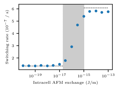
Figure 1: Datapoints show simulated switching rates ,using mumax⁺, of an antiferromagnet with a saturation magnetization of $M_{s}=400\,\mathrm{kA/m}$ and an uniaxial anisotropy constant $K_{u1}=2.5\,\mathrm{kJ/m^{3}}$ as a function of the antiferromagnetic coupling constant $A_{0}$. The dashed lines show simulated results of the switching rate of a ferromagnet. In the limit of low $A_{0}$, the antiferromagnetic system behaves as a ferromagnet with the same $M_{s}$ and $K_{u1}$. In the limit of high coupling, the datapoints approximate the switching rate of a ferromagnet with $2M_{s}$ and $2K_{u1}$.

3.2 Elasticity

Based on a previous extension of mumax³ [14], the mumax⁺ timesolver can also solve the second order elastodynamic equation [27, 28]

$$\rho\frac{\partial^{2}\mathbf{u}}{\partial^{2}t}=\mathbf{f}_{\text{tot}},$$ (10)

or equivalently the two first order differential equations

$$\begin{split}\partialderivative{\mathbf{u}}{t}&=\mathbf{v}\\ \partialderivative{\mathbf{v}}{t}&=\mathbf{a}=\frac{\mathbf{f}_{\text{tot}}}{\rho},\end{split}$$ (11)

with $\mathbf{u}$ the elastic displacement, $\mathbf{v}$ the velocity, $\mathbf{a}$ the acceleration, $\rho$ the mass density and $\mathbf{f}_{\text{tot}}$ the total body force density. It contains a damping force $\mathbf{f}_{\text{d}}=-\eta\mathbf{v}$ with a phenomenological damping parameter $\eta$, an external force $\mathbf{f}_{\text{ext}}$ set by the user, and the elastic body force $\mathbf{f}_{\text{el}}=\divergence{\hat{\mathbf{\sigma}}}$. The second order mechanical stress tensor $\hat{\mathbf{\sigma}}$ is given by Hooke’s law $\hat{\mathbf{\sigma}}=\hat{\mathbf{c}}:\hat{\mathbf{\varepsilon}}$, where $\hat{\mathbf{c}}$ is the fourth order stiffness tensor and $\hat{\mathbf{\varepsilon}}=\frac{1}{2}\left(\gradient\mathbf{u}+\left(\gradient\mathbf{u}\right)^{\intercal}\right)$ is the symmetric second order strain tensor. The material is assumed to have a cubic crystal structure, so $\hat{\mathbf{c}}$ can be described fully by three components of the stiffness tensor in reduced dimensionality (Voigt notation): $C_{11}$, $C_{12}$ and $C_{44}$.

Unlike in the previous implementation of Ref. [14], the numerical implementation of the elastic force $\mathbf{f}_{\text{el}}$ does not use written-out second order differentials of the elastic displacement. Rather, the strain is computed numerically using the gradient of the displacement, then the force is computed numerically as the divergence of the stress. In this way, traction-free boundary conditions are easily implemented, where $\hat{\mathbf{\sigma}}\cdot\mathbf{n}=\mathbf{0}$ applies at the boundary, with $\mathbf{n}$ the normal to the boundary. Future expansion of the code is also easier, for example to use a generalized stiffness tensor or to add additional strain terms such as piezoelectric strain. Lastly, the accuracy is higher, as both spatial derivative calculations utilize a fourth order accurate central difference scheme [29].

3.3 Magnetoelasticity

Magnetoelasticity for ferromagnets is implemented exactly as described in Ref. [14]. It is the combination of magnetostriciton [30], where the magnetization affects the elastic behaviour of the material, and the Villari effect or inverse magnetostriction [30], where the elastic strain affects the magnetization. For materials with cubic crystal symmetry, the first effect is described by an additional body force density

$$\mathbf{f}_{\text{mel}}=2B_{1}\matrixquantity[m_{x}\partialderivative{m_{x}}{x}\\ m_{y}\partialderivative{m_{y}}{y}\\ m_{z}\partialderivative{m_{z}}{x}]+B_{2}\matrixquantity[m_{x}\left(\partialderivative{m_{y}}{y}+\partialderivative{m_{z}}{z}\right)+m_{y}\partialderivative{m_{x}}{y}+m_{z}\partialderivative{m_{x}}{z}\\ m_{y}\left(\partialderivative{m_{x}}{x}+\partialderivative{m_{z}}{z}\right)+m_{x}\partialderivative{m_{y}}{x}+m_{z}\partialderivative{m_{y}}{z}\\ m_{z}\left(\partialderivative{m_{x}}{x}+\partialderivative{m_{y}}{y}\right)+m_{x}\partialderivative{m_{z}}{x}+m_{y}\partialderivative{m_{z}}{y}\\ ],$$ (12)

while the second effect adds a magnetoelastic field $\mathbf{B}_{\text{mel}}$ to the effective field $\mathbf{B}_{\text{eff}}$.

$$\mathbf{B}_{\text{mel}}=-\frac{2}{M_{s}}\left(B_{1}\matrixquantity[\varepsilon_{xx}m_{x}\\ \varepsilon_{yy}m_{y}\\ \varepsilon_{zz}m_{z}]+B_{2}\matrixquantity[\varepsilon_{xy}m_{y}+\varepsilon_{xz}m_{z}\\ \varepsilon_{xy}m_{x}+\varepsilon_{yz}m_{z}\\ \varepsilon_{xz}m_{x}+\varepsilon_{yz}m_{y}\\ ]\right)$$ (13)

$B_{1}$ and $B_{2}$ are the first and second magnetoelastic coupling constants and $\varepsilon_{ij}$ are the components of the strain tensor $\hat{\mathbf{\varepsilon}}$.

Magnetoelasticity for antiferromagnets and ferrimagnets is implemented similarly to Ref. [31]. The whole magnet has a shared elastic displacement, velocity, stiffness and body force, while each ferromagnetic sublattice $s$ has its own magnetoelastic coupling constants $B_{1}^{(s)}$ and $B_{2}^{(s)}$ and uses its own magnetization $\mathbf{m^{(s)}}$ and saturation magnetization $M_{s}^{(s)}$. Each sublattice then creates a magnetoelastic body force $\mathbf{f}_{\text{mel}}^{(s)}$, which is added to the total body force $\mathbf{f}_{\text{tot}}$. Conversely, each sublattice magnetization is affected by a unique magnetoelastic field $\mathbf{B}_{\text{mel}}^{(s)}$ created by its magnetization $\mathbf{m}^{(s)}$ and the shared strain $\hat{\mathbf{\varepsilon}}$.

3.4 Time integration

For the numerical time integration of the dynamical equations, mumax⁺ utilizes several Runge-Kutta methods with the option to use adaptive time stepping. However, at the time of writing, the adaptive time stepping should not be used when performing magnetoelastic simulations, due to the different scales of the velocity and acceleration, Eq. (11), and torque, Eq. (1). In those cases the time steps should be set to a constant value. In Tab. 1 we show the methods currently available with their convergence order and the order of the error estimate, which is used for adaptive time stepping. The Fehlberg method is the default solver in mumax⁺ and all methods are implemented by using their butcher tableaux, making it relatively easy to add more.

Table 1: Runge-Kutta solvers in mumax⁺ together with their convergence order and error estimate order which is used for adaptive time stepping.

Method	Convergence order	Error estimate order
Heun (RK12)	2	1
Bogacki-Shampine (RK23)	3	2
Cash-Karp	5	4
Fehlberg (RKF45)	5	4
Dormand-Prince (RK45)	5	4

Besides the standard time integration using butcher tableaux, mumax⁺ also provides a minimize and relax function to find the system’s energy minimum. The implementation of both is similar as in mumax³. In order to find the energy minimum of an antiferromagnet, the algorithms considers both sublattices and their energy is minimized simultaneously.

4 Verification

The mumax⁺ software was thoroughly tested with the different micromagnetic standard problems [15], physical and analytical results and by comparing it with results from mumax³. These tests can be found in the Github repository and can be run using pytest [32]. Since the implementation of antiferromagnets and elastodynamics forms an extension of the main mumax³ physics, the remainder of this section will treat the verification of these two features.

4.1 Width of domain wall stabilized by interfacial DMI

In Ref. [21] it is shown that an antiferromagnetic domain wall can be stabilized by interfacial DMI in a thin film antiferromagnet with uniaxial out-of-plane anisotropy. The authors give an analytical derivation of the static domain wall width, which results in [21]

$$\Delta=\sqrt{\frac{2A_{11}-A_{12}}{2K_{u1}}}\,.$$ (14)

We compare this result with simulations performed with mumax⁺. Figure 2 shows the domain wall width in the same system as considered in Ref. [21] for a range of different material parameters. The results from mumax⁺ agree well with the analytical result in equation (14). This forms a test of the implementation of both the different exchange terms given in equation (3) and the DMI in antiferromagnetic systems.

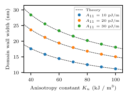
Figure 2: Figure shows domain wall widths simulated with mumax⁺ in an antiferromagnetic thin-film consisting of $200\times 100\times 1$ cubic cells with a length of $2\,\mathrm{nm}$ with varying uniaxial anisotropy and inhomogeneous ferromagnetic exchange constants, $K_{u1}$ and $A_{11}$ respectively. The sublattices have a saturation magnetization of $0.4\,\mathrm{MA/m}$ and antiferromagnetic exchange coupling constants of $A_{0}=-25\,\mathrm{pJ/m}$ and $A_{12}=-5\,\mathrm{pJ/m}$. The domain wall is stabilized by an interfacial DMI with a strength of $0.11\,\mathrm{mJ/m^{2}}$. The results correspond well to the analytical description given in Ref. [21] and shown in Eq. 14.

4.2 Current driven domain wall motion in antiferromagnets

The system mentioned in figure 2 and described in Ref. [21] can be investigated further by applying a current to the antiferromagnetic thin film. mumax⁺ forms a tool to investigate such dynamics. An analytical derivation of the domain wall velocity is derived in Ref. [21] and given by

$$v=\Delta(J)\cdot\frac{\pi\gamma\hbar}{8e}\cdot\frac{PJ}{t\alpha M_{s}}\left(\cos\Phi^{(2)}-\cos\Phi^{(2)}\right)\,,$$ (15)

where $\hbar$, $e$, $t$, $P$ and $J$ are the reduced Planck’s constant, elementary charge, film thickness, current polarization and applied current respectively. $\Phi^{(s)}$ is the angle between the sublattice magnetization $\mathbf{m}^{(s)}$ and the $x$-axis. Figure 3shows simulation results of the domain wall velocity under different applied currents. These results correspond well to the ones obtained in Ref. [21] and given in Eq. 15.

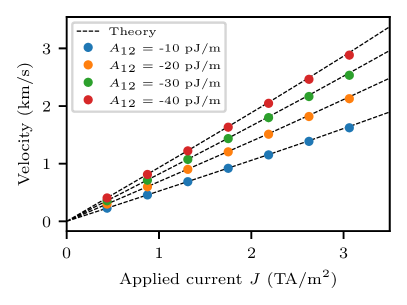
Figure 3: Figure shows domain wall velocities simulated with mumax⁺ in the same antiferromagnetic thin-film as in Fig. 2 for different applied currents and inhomogeneous antiferromagnetic exchange constants, $J$ and $A_{12}$ respectively. The applied current causes a Slonczewski spin-transfer torque with a polarization of $0.044$ and $\Lambda=1$ [5]. The anisotropy constant, ferromagnetic exchange constant and homogeneous antiferromagnetic exchange constant are held fixed at $64\,\mathrm{kJ/m^{3}}$, $2\,\mathrm{pJ/m}$ and $-2\mathrm{pJ/m}$ respectively. The results correspond well to the analytical description given in Ref. [21] and shown in Eq. 15.

4.3 Spinwaves in antiferromagnets

The dispersion relation for spinwaves in ferromagnets has been calculated in Refs. [33, 34, 35, 36]. The method can be extended to antiferromagnets. In this case there are two dynamic vector equations (1) with the LLG torque (2), one for each sublattice, which are coupled by the exchange fields (3). We assume a collinear antiferromagnet with uniaxial anisotropy $K_{u1}$ and an external field $B_{\text{ext}}$ in the $z$-direction. The demagnetizing field is assumed to be negligible due to the collinearity. The unperturbed magnetization lies along the $z$-direction and we apply a perturbation in the $x$- and $y$-direction. The resulting magnetization of the sublattices is then given by

$$\textbf{m}^{(1)}=\begin{bmatrix}0\\ 0\\ 1\end{bmatrix}+\begin{bmatrix}m_{x}^{(1)}\\ m_{y}^{(1)}\\ 0\end{bmatrix}e^{i(\omega t+\mathbf{k}\cdot\mathbf{r})},\qquad\textbf{m}^{(2)}=\begin{bmatrix}0\\ 0\\ -1\end{bmatrix}+\begin{bmatrix}m_{x}^{(2)}\\ m_{y}^{(2)}\\ 0\end{bmatrix}e^{i(\omega t+\mathbf{k}\cdot\mathbf{r})}.$$ (16)

The dispersion relation can now be obtained by calculating each component of the LLG equation up to first order in the perturbation for both sublattices. The result is a set of four equations given by

$$\begin{split}i\omega m_{x}^{(1)}+\left(\omega_{\text{ext}}+\omega_{\text{ani}}-\omega_{0}+\omega_{11}\right)m_{y}^{(1)}-\left(\omega_{0}-\omega_{12}\right)m_{y}^{(2)}&=0\\ i\omega m_{y}^{(1)}-\left(\omega_{\text{ext}}+\omega_{\text{ani}}-\omega_{0}+\omega_{11}\right)m_{x}^{(1)}+\left(\omega_{0}-\omega_{12}\right)m_{x}^{(2)}&=0\\ i\omega m_{x}^{(2)}+\left(\omega_{\text{ext}}-\omega_{\text{ani}}+\omega_{0}-\omega_{11}\right)m_{y}^{(2)}+\left(\omega_{0}-\omega_{12}\right)m_{y}^{(1)}&=0\\ i\omega m_{y}^{(2)}-\left(\omega_{\text{ext}}-\omega_{\text{ani}}+\omega_{0}-\omega_{11}\right)m_{x}^{(2)}-\left(\omega_{0}-\omega_{12}\right)m_{x}^{(1)}&=0.\end{split}$$ (17)

Here we defined

$$\omega_{\text{ext}}=\gamma B_{\text{ext}},\qquad\omega_{\text{ani}}=\gamma\frac{2K_{u1}}{M_{s}},\qquad\omega_{0}=\gamma\frac{4A_{0}}{a^{2}M_{s}},$$

$$\omega_{11}=\gamma\frac{2A_{11}}{M_{s}}k^{2},\qquad\omega_{12}=\gamma\frac{A_{12}}{M_{s}}k^{2},$$

where $M_{s}$, $K_{u1}$ and $A_{11}$ are identical for both sublattices. Notice that there are no equations for the $z$-component of the LLG equations, as these only contain terms of second order in the perturbations. This system of equations can also be rewritten in matrix notation with a $4\times 4$ matrix, resulting in

$$\begin{bmatrix}i\omega&\omega_{\text{ext}}+\omega_{b}&0&-\omega_{0}+\omega_{12}\\ -\omega_{\text{ext}}-\omega_{b}&i\omega&\omega_{0}-\omega_{12}&0\\ 0&\omega_{0}-\omega_{12}&i\omega&\omega_{\text{ext}}-\omega_{b}\\ -\omega_{0}+\omega_{12}&0&-\omega_{\text{ext}}+\omega_{b}&i\omega\end{bmatrix}\cdot\begin{bmatrix}m_{1,x}\\ m_{1,y}\\ m_{2,x}\\ m_{2,y}\end{bmatrix}=0,$$

where

$$\omega_{b}=\omega_{\text{ani}}-\omega_{0}+\omega_{11}.$$

Nontrivial solutions of the system are found only when the determinant is equal to zero. This expression yields the four dispersion relations for a bulk antiferromagnet.

$$\omega=\pm\sqrt{(\omega_{\text{ani}}+\omega_{11}-\omega_{12})(\omega_{\text{ani}}+\omega_{11}-2\omega_{0}+\omega_{12})}\pm\omega_{\text{ext}}.$$ (18)

The anisotropy creates an energy gap, while the external field lifts the degeneracy. In absence of anisotropy, $\omega_{\text{ani}}=$0\text{\,}\mathrm{THz}\text{/}\mathrm{rad}$$, the dispersion relation becomes characteristically linear [37, 38, 39] for small values of the wave number $k$.

$$\omega\approx\pm\frac{\gamma}{M_{s}}\sqrt{-8\frac{A_{0}}{a^{2}}\left(2A_{11}-A_{12}\right)}\absolutevalue{k}\,\pm\,\omega_{\text{ext}},\qquad k\ll\sqrt{\frac{-8A_{0}/a^{2}}{2A_{11}+A_{12}}}$$ (19)

To check if mumax⁺ obtains the same dispersion relation, we ran a simulation of a wire containing $512$ cubic cells with a length of $0.5\text{\,}\mathrm{nm}\text{/}$ and a lattice parameter $a$ of $3.5\text{\,}\mathrm{\SIUnitSymbolAngstrom}\text{/}$. The magnet has a saturation magnetization of $400\text{\,}\mathrm{kA}\text{/}\mathrm{m}$ and the exchange parameters are $A_{11}=$10\text{\,}\mathrm{pJ}\text{/}\mathrm{m}$$, $A_{0}=$-400\text{\,}\mathrm{pJ}\text{/}\mathrm{m}$$, $A_{12}=$-5\text{\,}\mathrm{pJ}\text{/}\mathrm{m}$$. The uniaxial anisotropy has a value of $1\text{\,}\mathrm{k}\mathrm{J}\mathrm{/}\mathrm{m}^{3}$ and the external field has a strength of $0.4\text{\,}\mathrm{T}\text{/}$. The simulation ran for $2\text{\,}\mathrm{ps}\text{/}$, during which a magnetic field sinc pulse was applied in the wire direction. A temporal and spatial Fourier transform of the magnetization of one of the sublattices was then taken and the result is shown in Fig. 4. This result shows a good correspondence between mumax⁺ and the theoretical result in Eq. 18.

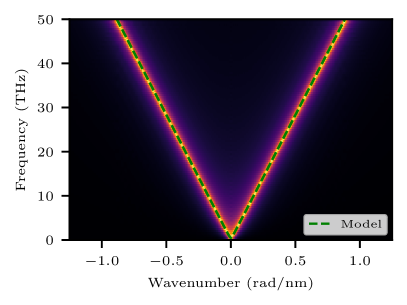
Figure 4: Dispersion relation obtained with mumax⁺ and compared with the analytical result (green curve). The parameters are given in the text.

4.4 Magnetoelastic waves in antiferromagnets

To calculate the dispersion relation of elastic waves, the following wave-like ansatz can be inserted in the elastodynamic equation (10).

$$\textbf{u}=\left[u_{x},\,u_{y},\,u_{z}\right]^{\intercal}e^{i(\omega t+\mathbf{k}\cdot\mathbf{r})}.$$ (20)

Assuming an isotropic stiffness tensor, $C_{12}$ can be replaced by $C_{11}-2C_{44}$, which simplifies the calculation. This has already been done in Ref. [33, 40] and the authors found three solutions. One of these corresponds to a longitudinal wave with a dispersion relation given by $\omega_{l}=\sqrt{\frac{C_{11}}{\rho}}k$ and the other two correspond to transversal waves with a dispersion relation given by $\omega_{t}=\sqrt{\frac{C_{44}}{\rho}}k$.

Analogously to Ref. [33], magnetoelastic waves in antiferromagnets are created by coupling the elastodynamic equation (10) to the two sublattice LLG equations (1, 2). As described in Section 3.3, this is done by incorporating the magnetoelastic body forces of both sublattices $\mathbf{f}_{\text{mel}}^{(s)}$ into the total body force $\mathbf{f}_{\text{tot}}$ and by adding the respective magnetoelastic fields $\mathbf{B}_{\text{mel}}^{(s)}$ (13) to the effective fields $\mathbf{B}_{\text{eff}}^{(s)}$. The elastic and spin waves will mutually interact with each other, resulting in the anticrossing of the elastic and magnetic dispersion relations [36, 41], characterized by the formation of a gap.

The uniaxial anisotropy, external field and magnetizations are still assumed to lie in the $z$-direction as in Section 4.3, and we assume a combined wave-like solution with equations (16) and (20). The remaining $xy$-plane isotropy lets us choose the $\mathbf{k}$-vector in the $xz$-plane without loss of generality, with $\mathbf{k}=\left[k\sin(\theta),0,k\cos(\theta)\right]^{\intercal}$. The $x$ and $z$ displacement components are rewritten in components along ($u_{l}$) and perpendicular to ($u_{t}$) the wave propagation $\mathbf{k}$. Neglecting non-linear terms yields the following set of coupled differential equations.

$$\begin{split}\left(\omega^{2}-\omega_{l}^{2}\right)\sin(\theta)u_{l}+\left(\omega^{2}-\omega_{H}^{2}\right)\cos(\theta)u_{t}+\frac{iB_{2}k\cos(\theta)}{\rho}\left(m_{x}^{(1)}-m_{x}^{(2)}\right)&=0\\ \left(\omega^{2}-\omega_{V}^{2}\right)u_{y}+\frac{iB_{2}k\cos(\theta)}{\rho}\left(m_{y}^{(1)}-m_{y}^{(2)}\right)&=0\\ \left(\omega^{2}-\omega_{l}^{2}\right)\cos(\theta)u_{l}-\left(\omega^{2}-\omega_{H}^{2}\right)\sin(\theta)u_{t}+\frac{iB_{2}k\sin(\theta)}{\rho}\left(m_{x}^{(1)}-m_{x}^{(2)}\right)&=0\\ i\gamma\frac{B_{2}}{M_{s}}k\cos(\theta)u_{y}+i\omega m_{x}^{(1)}+(\omega_{\text{ext}}+\omega_{b})m_{y}^{(1)}-(\omega_{0}-\omega_{12})m_{y}^{(2)}&=0\\ -i\gamma\frac{B_{2}}{M_{s}}k[\sin(2\theta)u_{l}+\cos(2\theta)u_{t}]+i\omega m_{y}^{(1)}-(\omega_{\text{ext}}+\omega_{b})m_{x}^{(1)}+(\omega_{0}-\omega_{12})m_{x}^{(2)}&=0\\ i\gamma\frac{B_{2}}{M_{s}}k\cos(\theta)u_{y}+i\omega m_{x}^{(2)}+(\omega_{\text{ext}}-\omega_{b})m_{y}^{(2)}+(\omega_{0}-\omega_{12})m_{y}^{(1)}&=0\\ -i\gamma\frac{B_{2}}{M_{s}}k[\sin(2\theta)u_{l}+\cos(2\theta)u_{t}]+i\omega m_{y}^{(2)}-(\omega_{\text{ext}}-\omega_{b})m_{x}^{(2)}-(\omega_{0}-\omega_{12})m_{x}^{(1)}&=0.\end{split}$$ (21)

Writing this in matrix notation with a $7\times 7$ matrix and setting the determinant equal to zero results in the implicit magnetoelastic dispersion relation of the form

$$\begin{gathered}2Jk^{2}\omega_{\text{ag}}\cos^{2}(\theta)\Bigl{\{}Jk^{2}\omega_{\text{ag}}(\omega_{l}^{2}+\omega_{H}^{2}-2\omega^{2})\\ -(\omega_{l}^{2}-\omega^{2})(\omega_{H}^{2}-\omega^{2})\bigl{[}\omega_{\text{mag}}^{2}-\omega_{\text{ext}}^{2}-\omega^{2}\bigr{]}\\ +Jk^{2}\omega_{\text{ag}}(\omega_{l}^{2}-\omega_{H}^{2})\cos(4\theta)\Bigr{\}}\\ +(\omega_{V}^{2}-\omega^{2})\Bigl{\{}-Jk^{2}\omega_{\text{ag}}(\omega_{l}^{2}+\omega_{H}^{2}-2\omega^{2})\bigl{[}\omega_{\text{mag}}^{2}-\omega_{\text{ext}}^{2}-\omega^{2}\bigr{]}\\ +(\omega_{l}^{2}-\omega^{2})(\omega_{H}^{2}-\omega^{2})\bigl{[}\omega_{\text{mag}}^{2}-(\omega_{\text{ext}}-\omega)^{2}\bigr{]}\bigl{[}\omega_{\text{mag}}^{2}-(\omega_{\text{ext}}+\omega)^{2}\bigr{]}\\ -Jk^{2}\omega_{\text{ag}}(\omega_{l}^{2}-\omega_{H}^{2})\bigl{[}\omega_{\text{mag}}^{2}-\omega_{\text{ext}}^{2}-\omega^{2}\bigr{]}\cos(4\theta)\Bigr{\}}\\ =0.\end{gathered}$$ (22)

Here we introduced

$$\omega_{\text{mag}}^{2}=\omega_{\text{m}}\omega_{\text{ag}}=\left(\omega_{\text{ani}}+\omega_{11}-\omega_{12}\right)\left(\omega_{\text{ani}}+\omega_{11}+\omega_{12}-2\omega_{0}\right),$$

$$\omega_{H}=\omega_{V}=\omega_{t},\qquad J=\frac{\gamma B_{2}^{2}}{\rho M_{s}}.$$

$\omega_{\text{H}}$ and $\omega_{\text{V}}$ are the angular frequencies of the horizontally ($u_{t}$) and vertically ($u_{y}$) polarized transversal elastic waves, respectively. Both are equal to $\omega_{\text{t}}$ due to the isotropic stiffness, but are kept separate for interpretation.

In mumax⁺ we simulate a wire consisting of $4096$ cells of $1\text{\,}{\mathrm{nm}}^{3}\text{/}$ with periodic boundary conditions. The used parameters are based on MnPS3, with $M_{s}=$566\text{\,}\mathrm{kJ}\text{/}\mathrm{m}$$ [31], $a=$0.61\text{\,}\mathrm{nm}\text{/}$$, $K_{u1}=$611\text{\,}\mathrm{k}\mathrm{J}\mathrm{/}\mathrm{m}^{3}$$ [42], $A_{11}=$2.48\text{\,}\mathrm{pJ}\text{/}\mathrm{m}$$, $A_{0}/a^{2}=$-0.993\text{\,}\mathrm{M}\mathrm{J}\mathrm{/}\mathrm{m}^{3}$$ and $A_{12}=$0\text{\,}\mathrm{J}\text{/}\mathrm{m}$$ [31]. The elastic parameters are chosen to be $\rho=$2800\text{\,}\mathrm{k}\mathrm{g}\mathrm{/}\mathrm{m}^{3}$$ [43], $C_{11}=$200\text{\,}\mathrm{GPa}\text{/}$$, $C_{44}=$70\text{\,}\mathrm{GPa}\text{/}$$ [42], $C_{12}=C_{11}-2C_{44}=$60\text{\,}\mathrm{GPa}\text{/}$$ [33] and $B_{1}=B_{2}=$-5.5\text{\,}\mathrm{M}\mathrm{J}\mathrm{/}\mathrm{m}^{3}$$ [33, 42]. The applied external field has a strength of $2\text{\,}\mathrm{T}\text{/}$, which has an angle $\theta$ of $30\text{\,}\mathrm{\SIUnitSymbolDegree}\text{/}$ with the wave propagation. This magnitude is low enough to avoid the spin-flop transition, but strong enough to clearly lift the degeneracy. We simulate $0.8\text{\,}\mathrm{ns}\text{/}$ while a magnetic field and an external force sinc pulse is applied in every direction. A Fourier transform is then applied to the space- and time-dependent magnetization and displacement components. The result of this simulation can be seen in Fig. 5 together with the analytical solutions of the uncoupled and coupled system.

The results show that mumax⁺ corresponds very well to the theory. There is clear anticrossing behavior at multiple points, showing the correct interaction between the elastic and spin waves. Even the lifting of the degeneracy between the horizontally ($\omega_{H}$) and vertically ($\omega_{V}$) polarized transversal elastic waves can be seen. There is an additional straight line at $k=$0\text{\,}\mathrm{r}\mathrm{a}\mathrm{d}\mathrm{/}\mathrm{n}\mathrm{m}$$ however. This is only present in the Fourier transform of the displacement and is the result of a translation of the entire system.

In the case of wave propagation perpendicular to the magnetization with $\theta=$90\text{\,}\mathrm{\SIUnitSymbolDegree}\text{/}$$, the vertically polarized and longitudinal elastic waves are uncoupled, while the horizontally polarized waves remain coupled to the spinwaves. This can be seen by simplifying Eq. 22, which results in

$$\begin{gathered}(\omega_{l}^{2}-\omega^{2})(\omega_{V}^{2}-\omega^{2})\Bigl{\{}-2Jk^{2}\omega_{\text{ag}}(\omega_{\text{mag}}^{2}-\omega_{ext}^{2}-\omega^{2})\\ +(\omega_{H}^{2}-\omega^{2})\bigl{[}\omega_{\text{mag}}^{2}-(\omega_{ext}-\omega)^{2}\bigr{]}\bigl{[}\omega_{\text{mag}}^{2}-(\omega_{ext}+\omega)^{2}\bigr{]}\bigr{\}}=0.\end{gathered}$$ (23)

This can also be clearly seen in the simulation results of Fig. 6, where the anticrossing is only observed between the spinwaves and one of the transversal elastic waves, while the other elastic wave dispersion relations remain unchanged. This result qualitatively corresponds well to the theoretical results for small wave numbers obtained in Refs. [42, 44].

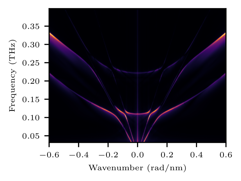
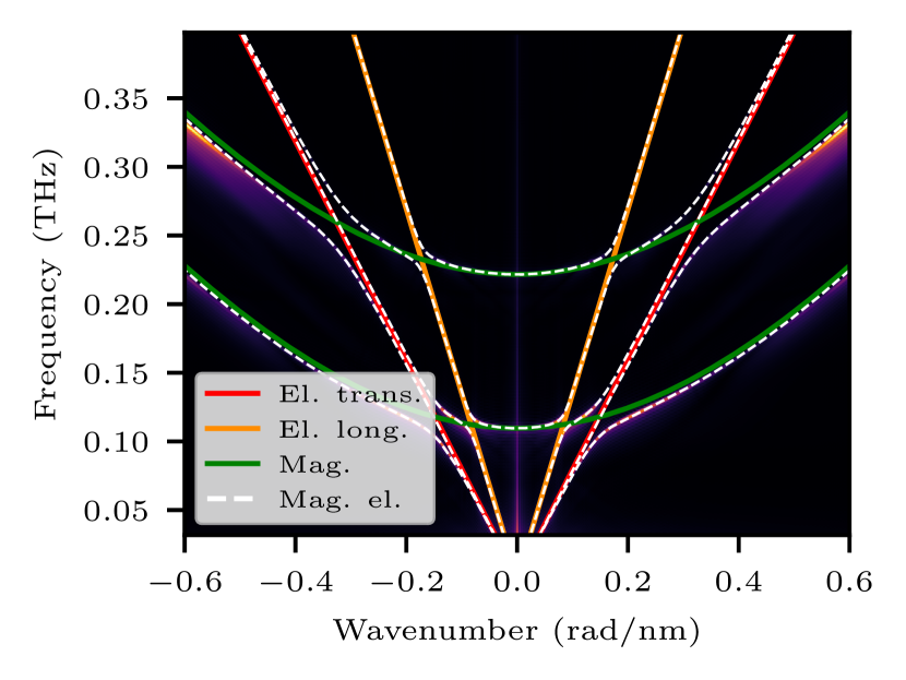
Figure 5: Magnetoelastic dispersion relation for antiferromagnets simulated with mumax⁺. The red, orange and green curves are the transversal elastic, longitudinal elastic and magnetic dispersion relations without magnetoelastic coupling respectively. The white dashed line is the analytical solution of the coupled dispersion relation. The parameters are given in the text and the angle between the wave propagation and the external field is $30\text{\,}\mathrm{\SIUnitSymbolDegree}\text{/}$.

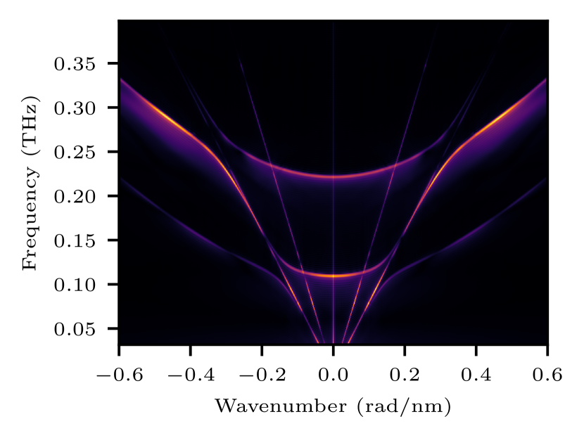
Figure 6: Magnetoelastic dispersion relation for antiferromagnets simulated with mumax⁺. The red, orange and green curves are the transversal elastic, longitudinal elastic and magnetic dispersion relations without magnetoelastic coupling respectively. The white dashed line is the analytical solution of the coupled dispersion relation. The parameters are given in the text and the angle between the wave propagation and the external field is $90\text{\,}\mathrm{\SIUnitSymbolDegree}\text{/}$.

5 Conclusions and outlook

We presented the micromagnetic model employed by mumax⁺ and how it differs from its predecessor mumax³. These differences include a Python based interface, the ability to perform calculations using antiferromagnets and ferrimagnets, and magnetoelasticity for every type of magnet in the package. These new tools have been verified by performing comparisons with analytical results and by deriving an antiferromagnetic magnetoelastic dispersion relation.

The development and maintenance of mumax⁺ is ongoing and many more functionalities are expected in future releases. Some possibilities include non-collinear antiferromagnets, adaptive time stepping for magnetoelastic simulations, a more general stiffness tensor and piezoelectric coupling. Since mumax⁺ is open source and built with an object-oriented design for easy extensibility, anyone can, in principle, fork the repository and enhance the module with additional features.

References

- \bibcommenthead
- Donahue [1999] Donahue, M.: OOMMF User’s Guide, Version 1.0. - 6376, National Institute of Standards and Technology, Gaithersburg, MD (1999). https://doi.org/10.6028/NIST.IR.6376
- Vansteenkiste and Van de Wiele [2011] Vansteenkiste, A., Van de Wiele, B.: Mumax: A new high-performance micromagnetic simulation tool. Journal of Magnetism and Magnetic Materials 323(21), 2585–2591 (2011) https://doi.org/10.1016/j.jmmm.2011.05.037
- Vansteenkiste et al. [2012] Vansteenkiste, A., Van de Wiele, B., Dvornik, M., Lassalle-Balier, R., Rowlands, G.: mumax2 (2012). https://github.com/mumax/2
- Scholz et al. [2003] Scholz, W., Fidler, J., Schrefl, T., Suess, D., Dittrich, R., Forster, H., Tsiantos, V.: Scalable parallel micromagnetic solvers for magnetic nanostructures. Computational Materials Science 28(2), 366–383 (2003) https://doi.org/%****␣sn-article.bbl␣Line␣100␣****10.1016/S0927-0256(03)00119-8 . Proceedings of the Symposium on Software Development for Process and Materials Design
- Vansteenkiste et al. [2014] Vansteenkiste, A., Leliaert, J., Dvornik, M., Helsen, M., Garcia-Sanchez, F., Van Waeyenberge, B.: The design and verification of MuMax3. AIP Advances 4(10), 107133 (2014) https://doi.org/10.1063/1.4899186
- Chang et al. [2011] Chang, R., Li, S., Lubarda, M.V., Livshitz, B., Lomakin, V.: Fastmag: Fast micromagnetic simulator for complex magnetic structures (invited). Journal of Applied Physics 109(7), 07–358 (2011) https://doi.org/10.1063/1.3563081 https://pubs.aip.org/aip/jap/article-pdf/doi/10.1063/1.3563081/16748870/07d358_1_online.pdf
- Kakay et al. [2010] Kakay, A., Westphal, E., Hertel, R.: Speedup of fem micromagnetic simulations with graphical processing units. IEEE Transactions on Magnetics 46(6), 2303–2306 (2010) https://doi.org/10.1109/TMAG.2010.2048016
- Lepadatu [2020] Lepadatu, S.: Boris computational spintronics—high performance multi-mesh magnetic and spin transport modeling software. Journal of Applied Physics 128(24), 243902 (2020) https://doi.org/10.1063/5.0024382
- Van Rossum and Drake [2009] Van Rossum, G., Drake, F.L.: Python 3 Reference Manual. CreateSpace, Scotts Valley, CA (2009)
- Harris et al. [2020] Harris, C.R., Millman, K.J., Walt, S.J., Gommers, R., Virtanen, P., Cournapeau, D., Wieser, E., Taylor, J., Berg, S., Smith, N.J., Kern, R., Picus, M., Hoyer, S., Kerkwijk, M.H., Brett, M., Haldane, A., Río, J.F., Wiebe, M., Peterson, P., Gérard-Marchant, P., Sheppard, K., Reddy, T., Weckesser, W., Abbasi, H., Gohlke, C., Oliphant, T.E.: Array programming with NumPy. Nature 585(7825), 357–362 (2020) https://doi.org/10.1038/s41586-020-2649-2
- Virtanen et al. [2020] Virtanen, P., Gommers, R., Oliphant, T.E., Haberland, M., Reddy, T., Cournapeau, D., Burovski, E., Peterson, P., Weckesser, W., Bright, J., van der Walt, S.J., Brett, M., Wilson, J., Millman, K.J., Mayorov, N., Nelson, A.R.J., Jones, E., Kern, R., Larson, E., Carey, C.J., Polat, İ., Feng, Y., Moore, E.W., VanderPlas, J., Laxalde, D., Perktold, J., Cimrman, R., Henriksen, I., Quintero, E.A., Harris, C.R., Archibald, A.M., Ribeiro, A.H., Pedregosa, F., van Mulbregt, P., SciPy 1.0 Contributors: SciPy 1.0: Fundamental Algorithms for Scientific Computing in Python. Nature Methods 17, 261–272 (2020) https://doi.org/10.1038/s41592-019-0686-2
- [12] The C++ programming language (2024). https://cplusplus.com/
- [13] NVIDIA CUDA C programming guide (2024). https://docs.nvidia.com/cuda/index.html
- Vanderveken et al. [2021] Vanderveken, F., Mulkers, J., Leliaert, J., Van Waeyenberge, B., Sorée, B., Zografos, O., Zografos, O., Ciubotaru, F., Adelmann, C.: Finite difference magnetoelastic simulator. Open Research Europe 1(35) (2021) https://doi.org/%****␣sn-article.bbl␣Line␣300␣****10.12688/openreseurope.13302.1
- [15] muMAG Micromagnetic Modeling Activity Group. https://www.ctcms.nist.gov/~rdm/mumag.org.html
- Zhang and Li [2004] Zhang, S., Li, Z.: Roles of nonequilibrium conduction electrons on the magnetization dynamics of ferromagnets. Phys. Rev. Lett. 93, 127204 (2004) https://doi.org/10.1103/PhysRevLett.93.127204
- Slonczewski [1996] Slonczewski, J.C.: Current-driven excitation of magnetic multilayers. Journal of Magnetism and Magnetic Materials 159(1), 1–7 (1996) https://doi.org/10.1016/0304-8853(96)00062-5
- Landau and Lifshitz [1935] Landau, L., Lifshitz, E.: On the theory of the dispersion of magnetic permeability in ferromagnetic bodies. reproduced in collected papers of ld landau. Pergamon, New York (1935)
- Gilbert [1955] Gilbert, T.L.: A lagrangian formulation of the gyromagnetic equation of the magnetization field. Phys. Rev. 100, 1243 (1955)
- Leliaert et al. [2017] Leliaert, J., Mulkers, J., De Clercq, J., Coene, A., Dvornik, M., Van Waeyenberge, B.: Adaptively time stepping the stochastic landau-lifshitz-gilbert equation at nonzero temperature: Implementation and validation in mumax3. AIP Advances 7(12), 125010 (2017) https://doi.org/10.1063/1.5003957 https://pubs.aip.org/aip/adv/article-pdf/doi/10.1063/1.5003957/19733887/125010_1_online.pdf
- Sánchez-Tejerina et al. [2020] Sánchez-Tejerina, L., Puliafito, V., Khalili Amiri, P., Carpentieri, M., Finocchio, G.: Dynamics of domain-wall motion driven by spin-orbit torque in antiferromagnets. Phys. Rev. B 101, 014433 (2020) https://doi.org/10.1103/PhysRevB.101.014433
- Hals and Everschor-Sitte [2017] Hals, K.M.D., Everschor-Sitte, K.: New boundary-driven twist states in systems with broken spatial inversion symmetry. Phys. Rev. Lett. 119, 127203 (2017) https://doi.org/10.1103/PhysRevLett.119.127203
- Mahfouzi and Kioussis [2022] Mahfouzi, F., Kioussis, N.: Bulk generalized dzyaloshinskii-moriya interaction in -symmetric antiferromagnets. Phys. Rev. B 106, 220404 (2022) https://doi.org/10.1103/PhysRevB.106.L220404
- Newell et al. [1993] Newell, A.J., Williams, W., Dunlop, D.J.: A generalization of the demagnetizing tensor for nonuniform magnetization. Journal of Geophysical Research: Solid Earth 98(B6), 9551–9555 (1993) https://doi.org/10.1029/93JB00694
- Chernyshenko and Fangohr [2015] Chernyshenko, D., Fangohr, H.: Computing the demagnetizing tensor for finite difference micromagnetic simulations via numerical integration. Journal of Magnetism and Magnetic Materials 381, 440–445 (2015) https://doi.org/10.1016/j.jmmm.2015.01.013
- Breth et al. [2012] Breth, L., Suess, D., Vogler, C., Bergmair, B., Fuger, M., Heer, R., Brueckl, H.: Thermal switching field distribution of a single domain particle for field-dependent attempt frequency. Journal of Applied Physics 112(2), 023903 (2012) https://doi.org/10.1063/1.4737413
- Graff [1975] Graff, K.F.: Wave motion in elastic solids. (1975). https://api.semanticscholar.org/CorpusID:137511754
- Achenbach [1973] Achenbach, J.D.: Wave Propagation in Elastic Solids. North-Holland Publishing Company/American Elsevier, Amsterdam (1973)
- Sauer and Sauer [2012] Sauer, T., Sauer, T.: Numerical Analysis. Always learning. Pearson, London (2012)
- Chikazumi [2009] Chikazumi, S.: Physics of Ferromagnetism. International Series of Monographs on Physics. OUP Oxford, Oxford (2009)
- Barra et al. [2018] Barra, A., Domann, J., Kim, K.W., Carman, G.: Voltage control of antiferromagnetic phases at near-terahertz frequencies. Phys. Rev. Appl. 9, 034017 (2018) https://doi.org/10.1103/PhysRevApplied.9.034017
- Krekel et al. [2004] Krekel, H., Oliveira, B., Pfannschmidt, R., Bruynooghe, F., Laugher, B., Bruhin, F.: pytest (2004). https://github.com/pytest-dev/pytest
- Vanderveken et al. [2021] Vanderveken, F., Ciubotaru, F., Adelmann, C.: In: Kamenetskii, E. (ed.) Magnetoelastic Waves in Thin Films, pp. 287–322. Springer, Cham (2021). https://doi.org/10.1007/978-3-030-62844-4_12
- Cottam [1994] Cottam, M.G.: Linear and Nonlinear Spin Waves in Magnetic Films and Superlattices. WORLD SCIENTIFIC, New Jersey (1994). https://doi.org/%****␣sn-article.bbl␣Line␣575␣****10.1142/1687
- Stancil and Prabhakar [2009] Stancil, D.D., Prabhakar, A.: Spin Waves: Theory and Applications. Springer, New York (2009)
- Gurevich and Melkov [1996] Gurevich, A.G., Melkov, G.A.: Magnetization Oscillations and Waves. Taylor & Francis, London (1996)
- Coey [2010] Coey, J.M.D.: Magnetism and Magnetic Materials. Magnetism and Magnetic Materials. Cambridge University Press, Cambridge (2010)
- Samuelsen and Shirane [1970] Samuelsen, E.J., Shirane, G.: Inelastic neutron scattering investigation of spin waves and magnetic interactions in -. physica status solidi (b) 42(1), 241–256 (1970) https://doi.org/%****␣sn-article.bbl␣Line␣625␣****10.1002/pssb.19700420125
- Samuelsen et al. [1970] Samuelsen, E.J., Hutchings, M.T., Shirane, G.: Inelastic neutron scattering investigation of spin waves and magnetic interactions in . Physica 48(1), 13–42 (1970) https://doi.org/10.1016/0031-8914(70)90158-8
- Achenbach [1973] Achenbach, J.D.: Wave Propagation in Elastic Solids. Applied Mathematics and Mechanics Series. North-Holland Publishing Company, Amsterdam (1973)
- Tucker and Rampton [1972] Tucker, J.W., Rampton, V.W.: Microwave Ultrasonics in Solid State Physics. Amsterdam : North-Holland, Amsterdam (1972)
- Zhang et al. [2020] Zhang, S., Go, G., Lee, K.-J., Kim, S.K.: Su(3) topology of magnon-phonon hybridization in 2d antiferromagnets. Phys. Rev. Lett. 124, 147204 (2020) https://doi.org/10.1103/PhysRevLett.124.147204
- Jain et al. [2013] Jain, A., Ong, S., Hautier, G., Chen, W., Richards, W., Dacek, S., Cholia, S., Gunter, D., Skinner, D., Ceder, G., Persson, K.: Commentary: The materials project: A materials genome approach to accelerating materials innovation. APL Materials 1, 011002 (2013) https://doi.org/10.1063/1.4812323
- Go et al. [2024] Go, G., Yang, H., Park, J.-G., Kim, S.K.: Topological magnon polarons in honeycomb antiferromagnets with spin-flop transition. Phys. Rev. B 109, 184435 (2024) https://doi.org/10.1103/PhysRevB.109.184435