Defective regression models for cure rate modeling in Marshall-Olkin family

Abstract

Regression model have a substantial impact on interpretation of treatments, genetic characteristics and other covariates in survival analysis. In many datasets, the description of censoring and survival curve reveals the presence of cure fraction on data, which leads to alternative modelling. The most common approach to introduce covariates under a parametric estimation are the cure rate models and their variations, although the use of defective distributions have introduced a more parsimonious and integrated approach. Defective distributions is given by a density function whose integration is not one after changing the domain of one the parameters. In this work, we introduce two new defective regression models for long-term survival data in the Marshall-Olkin family: the Marshall-Olkin Gompertz and the Marshall-Olkin inverse Gaussian. The estimation process is conducted using the maximum likelihood estimation and Bayesian inference. We evaluate the asymptotic properties of the classical approach in Monte Carlo studies as well as the behavior of Bayes estimates with vague information. The application of both models under classical and Bayesian inferences is provided in an experiment of time until death from colon cancer with a dichotomous covariate. The Marshall-Olkin Gompertz regression presented the best adjustment and we present some global diagnostic and residual analysis for this proposal.

1 Introduction

In survival analysis, the statistical analysis focuses on descriptions and inferences about the time until the occurrence of a specific event. This event, often referred as failure time, is a random variable defined on the non-negative real numbers. The fundamental assumption in failure time experiments is that all observed individuals will eventually experience the event of interest (Colosimo & Giolo, 2021). However, with advancements in medical treatments and pharmaceuticals, a significant portion of observed individuals tend to exhibit a cure for the outcome or recurrence of a disease (Maller & Zhou, 1996). Lin & Zhu (2008) discuss about this phenomena in reliability studies, where similarly situations arises when repair designs are incorporated into equipment to delay the failure time. Thus, assuming that the event of interest will occur for all sample units, despite the presence of a cure factor, leads to invalid inferences. Therefore, an alternative approach to traditional probabilistic models is necessary.

The first methodology introduced in the literature comprises the standard mixture models of Boag (1949) and Berkson & Gage (1952). These models adjust the survival function by adding a new parameter ($p$) to capture the fraction of cured individuals, as shown by $S(t)=p+(1-p)S_{0}(t)$, where $S_{0}(t)$ is a proper survival function. As $t\rightarrow\infty$, the survival function $S(t)$ converges to $p$. Additionally, there are variations of promotion time models in which the number of competing risks follows a Poisson distribution (Tsodikov et al., 1996), and an even more unified version where the number of competing causes follows a Negative Binomial distribution (Rodrigues et al., 2009).

A recent and integrated advancement in modeling data with a cure fraction lies in the study of defective models. This class is defined by a proper probability distribution that, upon modifying the natural parametric space of one of its parameters, becomes improper as it no longer integrates to one (Rodrigues, 2020). In practical scenarios, a defective model detects the presence of a cure fraction in the observations when one of its parameter takes a value outside the corresponding original parametric space. Otherwise, parameter estimation proceeds conventionally. In this regard, this framework provides a comprehensive approach to data with or without long-term survival times. If the model assumes a defective form, the survival function decreases to a constant value $1-p$, indicating the fraction of cured individuals in the observed data (Rodrigues, 2020). This can be estimated through a derived estimand ($i.e$., a function of the estimated parameters). In the literature, two distributions are widely applied: the Gompertz distribution and the Inverse Gaussian distribution. Both can adopt a defective version, with the primary advantage of requiring the estimation of one fewer parameter compared to standard cure models.

In the work of Rocha (2016), two new flexible defective distributions within the Marshall-Olkin family are introduced. The Marshall-Olkin family provides a framework for creating new probability distributions based on existing ones. Rocha (2016) demonstrates that, by employing the defective versions of the Gompertz and Inverse Gaussian distributions, the models within the Marshall-Olkin family also become defective. Mathematical properties of the Marshall-Olkin family are present in depth in the paper of Barreto-Souza et al. (2013). Under the frequentist approach, Rocha et al. (2016) presented simulation studies to evaluate the properties of maximum likelihood estimation and conducted model comparison experiments to demonstrate the ability to make accurate inferences for the Marshall-Olkin Gompertz and Marshall-Olkin Inverse Gaussian distributions. Three applications to different datasets were provided to showcase the practical performance of the defective versions compared to the mixture cure models for these two new distributions.

However, for data with a cured fraction, it is also interesting to investigate the effects of treatments, genetic characteristics, or other endogenous factors that may influence a patient’s immunity. Martinez & Achcar (2017) introduce the parametric regression under frequentist and Bayesian infereces for the defective generalized Gompertz model. An approach for interval-censored survival data with immune subjects for Gompertz and inverse Gaussian deffective distributions is discussed by Calsavara et al. (2019). Currently, there are no models in the literature with a regression structure that incorporate the Marshall-Olkin Gompertz and Marshall-Olkin Inverse Gaussian distributions. Therefore, the objective of this paper is to propose the Marshall-Olkin Gompertz and Marshall-Olkin Inverse Gaussian distributions as alternatives to comprehensive models for estimating the parametric survival function in the presence of a cured fraction in the population. In addition, this paper introduces the first approach under Bayesian paradigm for the two defective models proposed by Rocha (2016).

The remainder of the paper is organized as follows. Section 2 introduces the two new defective regression models as well as the inference methods. Section 3 presents simulation studies under both frequentist and Bayesian approaches. Section 4 includes an application to a colon cancer dataset. Conclusions are provided in Section 5.

2 Methodology

2.1 Classical defective distributions

Defective models represent a new approach to analyzing data from populations that contain immune individuals. Two commonly used defective distributions are the Gompertz distribution and the Inverse Gaussian distribution. There are more defective distributions distributions in literature, such as Dagum distribution (Martinez & Achcar, 2018), but this study prioritized the most applied in health studies.

According tGieser et al. (1998), the Gompertz distribution is one of the most widely used in studies of cure rates, especially when the hazard function is demonstrates an exponential behavior. Let $T$ be a random variable representing the time to failure following a Gompertz distribution. Its probability density function is

$$f(t\mid\alpha,\beta)=\beta e^{\alpha t}e^{-\frac{\beta}{\alpha}\left(e^{\alpha t}-1\right)},$$ (1)

for $\alpha>0$, $\beta>0$ and $t>0$. The corresponding survival function in the Gompertz distribution is

$$S(t\mid\alpha,\beta)=e^{-\frac{\beta}{\alpha}\left(e^{\alpha t}-1\right)}.$$ (2)

In the definition of Equation 1, the probability density function is proper. By changing the original parametric space of $\alpha$ to $(-\infty,0)$ the distribution becomes improper because it does not integrate 1. However, the cure fraction in data ($p$) can be easily computed as

$$p=\lim_{t\rightarrow\infty}S(t)=e^{\frac{\beta}{\alpha}}\in(0,1).$$

Once the values of $\alpha$ and $\beta$ are estimated, it is possible to obtain the cure fraction in data.

The inverse Gaussian is another usual alternative to survival modeling. Let $T$ be a random variable which represents the survival time following a inverse Gaussian distribution, its probability density function is given by

$$f(t\mid\alpha,\beta)=\frac{1}{\sqrt{2\beta\pi t^{3}}}e^{-\frac{1}{2\beta t}(1-\alpha t)^{2}},$$ (3)

for $\alpha>0$, $\beta>0$ and $t>0$. The reciprocal survival function is

$$S(t\mid\alpha,\beta)=1-\left[\Phi\left(\frac{\alpha t-1}{\sqrt{\beta t}}\right)+e^{\frac{2\alpha}{\beta}}\Phi\left(\frac{-(\alpha t+1)}{\sqrt{\beta t}}\right)\right],$$ (4)

where $\Phi$(.) denotes the cumulative distribution function of the standard normal distribution. The defective version of inverse Gaussian distribution is obtained by changing the domain of parameter $\alpha$ to $(-\infty,0)$. Consequently, the cumulative distribution function of inverse Gaussian does not integrate 1 anymore, becoming improper. Nevertheless, the cure fraction can be computed as

$$p=\lim_{t\rightarrow\infty}S(t)=\lim_{t\rightarrow\infty}\left(1-\left[\Phi\left(\frac{\alpha t-1}{\sqrt{\beta t}}\right)+e^{\frac{2\alpha}{\beta}}\Phi\left(\frac{-(\alpha t+1)}{\sqrt{\beta t}}\right)\right]\right)=1-e^{\frac{2\,\alpha}{\beta}}\in(0,1).$$

After the parameters $\alpha$ and $\beta$ being estimated, we can infer about the quantity of cure fraction in data.

2.2 The Marshal-Olkin family

The Marshall-Olkin famiky is a base field in probability distributions, in which is possible to create new flexible distributions based on the basal probability density function and basal cumulative distribution function of any well-defined distribution function in $\mathbb{R}$ with respect to Lebesgue measure. In the new structure, a parameter ($\lambda$) is added. Thus, the basal model is also included in this new group of distribution as a particular case (Marshall & Olkin, 1997).

Suppose that $S(t\mid\bm{\theta})$ and $f(t\mid\bm{\vartheta})$ are known probability density and survival functions, respectively, where $\bm{\theta}$ is the vector of parameters which identifies the statistical model. The extended version of survival function in the Marshal-Olkin Family is

$$S_{MO}(t\mid\bm{\theta},\lambda)=\dfrac{\lambda S(t\mid\bm{\theta})}{1-(1-\lambda)S(t\mid\bm{\vartheta})},$$ (5)

where $\lambda>0$ and $t>0$. Through the relationship between functions in survival analysis and derivations rules, we can obtain the probability density function in the Marshal-Olkin family given by

$$f_{MO}(t\mid\bm{\theta},\lambda)=\dfrac{\lambda f(t\mid\bm{\theta})}{\left[1-(1-\lambda)S(t\mid\bm{\theta})\right]^{2}}.$$ (6)

Rocha et al. (2016) proofs that $S_{MO}(t\mid\bm{\theta},\lambda)$ will be also defective if the basal $S(t\mid\bm{\theta})$ is defective, and this result enables the development of two new defective distributions: the Marshal-Olkin Gompertz and the Marshal-Olkin inverse Gaussian.

2.3 Marshal-Olkin Gompertz distribution

According to Rocha (2016), the survival function of Marshal-Olkin Gompertz model can be defined using the survival function in (2) in (5),

$$S(t\mid\alpha,\beta,\lambda)=\dfrac{\lambda e^{-\frac{\beta}{\alpha}\left(e^{\alpha t}-1\right)}}{1-(1-\lambda)e^{-\frac{\beta}{\alpha}\left(e^{\alpha t}-1\right)}}$$ (7)

for $\alpha>0$, $\beta>0$, $\lambda>0$, and $t>0$. Using the survival function in (2) and the probability density function in (1) of Gompertz distribution, the survival function of Marshall-Olkin Gompertz distribution can also be obtained as

$$f(t\mid\alpha,\beta,\lambda)=\dfrac{\lambda\beta e^{\alpha t}e^{-\frac{\beta}{\alpha}\left(e^{\alpha t}-1\right)}}{\left[1-(1-\lambda)e^{-\frac{\beta}{\alpha}\left(e^{\alpha t}-1\right)})\right]^{2}}.$$ (8)

Based on Gompertz distribution, if the parameter $\alpha<0$, the Marshall-Olkin Gompertz distribution is also defective. Its cure fraction is computed as

$$p=\lim_{t\rightarrow\infty}S(t)=\lim_{t\rightarrow\infty}\dfrac{\lambda e^{-\frac{\beta}{\alpha}\left(e^{\alpha t}-1\right)}}{1-(1-\lambda)e^{-\frac{\beta}{\alpha}\left(e^{\alpha t}-1\right)}}=\dfrac{\lambda p_{0}}{1-(1-\lambda)p_{0}},$$

where $p_{0}=e^{\frac{\beta}{\alpha}}$ is the cure fraction computed on the defective Gompertz distribution, commented in Section 2.1.

2.4 Marshal-Olkin inverse Gaussian distribution

Using the definition 5 and the survival function of inverse Gaussian distribution (4), the survival function of Marshall-Olkin inverse Gaussian distribution is

$$S(t\mid\alpha,\beta,\lambda)=\dfrac{\lambda\left(1-\left[\Phi\left(\frac{\alpha t-1}{\sqrt{\beta t}}\right)+e^{\frac{2\alpha}{\beta}}\Phi\left(\frac{-(\alpha t+1)}{\sqrt{\beta t}}\right)\right]\right)}{1-(1-\lambda)\left(1-\left[\Phi\left(\frac{\alpha t-1}{\sqrt{\beta t}}\right)+e^{\frac{2\alpha}{\beta}}\Phi\left(\frac{-(\alpha t+1)}{\sqrt{\beta t}}\right)\right]\right)},$$ (9)

for $\alpha>0$, $\beta>0$, $\lambda>0$, and $t>0$. Based on the Definition 6, the probability density function of Marshall-Olkin inverse Gaussian is

$$f(t\mid\alpha,\beta,\lambda)=\dfrac{\lambda e^{-\frac{1}{2\beta t}(1-\alpha t)^{2}}}{\sqrt{2\beta\pi t^{3}}\left[1-(1-\lambda)\left(1-\left[\Phi\left(\frac{\alpha t-1}{\sqrt{\beta t}}\right)+e^{\frac{2\alpha}{\beta}}\Phi\left(\frac{-(\alpha t+1)}{\sqrt{\beta t}}\right)\right]\right)\right]^{2}}.$$ (10)

The cure fraction informed by the defective Marshall-Olkin inverse Gaussian distribution is computed as

$$p=\lim_{t\rightarrow\infty}S(t)=\lim_{t\rightarrow\infty}\dfrac{\lambda\left(1-\left[\Phi\left(\frac{\alpha t-1}{\sqrt{\beta t}}\right)+e^{\frac{2\alpha}{\beta}}\Phi\left(\frac{-(\alpha t+1)}{\sqrt{\beta t}}\right)\right]\right)}{1-(1-\lambda)\left(1-\left[\Phi\left(\frac{\alpha t-1}{\sqrt{\beta t}}\right)+e^{\frac{2\alpha}{\beta}}\Phi\left(\frac{-(\alpha t+1)}{\sqrt{\beta t}}\right)\right]\right)}=\dfrac{\lambda p_{0}}{1-(1-\lambda)p_{0}},$$

where $p_{0}=1-e^{\frac{2\alpha}{\beta}}$ is the cure fraction calculated on defective inverse Gaussian distribution, presented in Section 2.1.

2.5 Model with covariates

Considering a survival experiment with periodic follow-ups and considering a sample of $n$ independent individuals with survival time, censoring and covariate information, the data set is expressed by $D=\left\{(t_{i},\delta_{i},\mathbf{X}_{i}):i=1,2,\dots,n\right\}$, where $t_{i}$ is the survival time registered, $\delta_{i}$ is the event indicator, and $\mathbf{X}_{i}$ is the covariate information for the $i-$th observation.

We include the covariate effects ($\mathbf{x}_{1}$) in the analysis to the shape parameter $\alpha$, which can be either positive (no cure fraction in data) or negative (presence of cure fraction in data), using the identity link function, that is,

$$\alpha(\mathbf{x}_{1i})={x}_{1i}^{\top}\bm{a},$$

where $\mathbf{x}_{1i}=(1,{x}_{1_{i1}},{x}_{1_{i2}},\dots,{x}_{1_{ip}})$ is a vector of observations from $p$ independent variables for the $i$-th observation and $\bm{a}=(a_{0},a_{1},\dots,a_{p})^{\top}$ is the vector of their corresponding regression coefficients. Similarly, covariate information ($\mathbf{x}_{2}$) can also be provided to the shape parameter $\beta>0$, because of its parametric domain, the logarithm link function is used,

$$\beta(\mathbf{x}_{2i},\mathbf{x}_{2i})=\exp({x}_{2i}^{\top}\mathbf{b}),$$

where $\mathbf{x}_{2i}=(1,{x}_{2_{i1}},{x}_{2_{i2}},\dots,{x}_{2_{iq}})$ is a vector of observations from $q$ independent variables for the $i$-th observation and $\bm{b}=(b_{0},b_{1},\dots,b_{q})^{\top}$ is the vector of their corresponding regression coefficients. Accordingly, the covariate information is defined as $\bm{X}_{i}=(\mathbf{x}_{1i},\mathbf{x}_{2i})$, $i=1,2,\dots,n$.

In the Marshall-Olkin defective models, it is also possible to introduce the covariate effects in the parameter $\lambda$; however, we opted to study the covariate information only in the scale ($\alpha$) and shape ($\beta$) parameters of basal distribution to model their basal cure fraction ($p_{0}$). For the Marshall-Olkin Gompertz regression, the $i-$th basal cure fraction is given by

$$p_{0_{i}}(\mathbf{x}_{1i},\mathbf{x}_{2i})=\exp\left(\dfrac{\exp({x}_{2i}^{\top}\mathbf{b})}{{x}_{1i}^{\top}\bm{a}}\right).$$

For the Marshall-Olkin inverse Gaussian regression, the $i-$th basal cure fraction is computed as

$$p_{0_{i}}(\mathbf{x}_{1i},\mathbf{x}_{2i})=1-\exp\left(2\,\dfrac{{x}_{1i}^{\top}\bm{a}}{\exp({x}_{2i}^{\top}\mathbf{b})}\right).$$

It is evident that, in both cases, $p_{0_{i}}(\mathbf{x}_{1i},\mathbf{x}_{2i})$ is an estimand of the vectors $\bm{a}=(a_{0},a_{1},\dots,a_{p})^{\top}$ and $\bm{b}=(b_{0},b_{1},\dots,b_{q})^{\top}$. Additionally, other link functions and regression structures can be proposed, but it is out of the scope of this study.

2.6 Frequentist Inference

Consider $T_{1},T_{2},\dots,T_{n}$ a sequence of $n$ independent non-negative random variables with survival function $S(.\mid\bm{\vartheta})$ and probability density function $f(.\mid\bm{\vartheta})$, indexed by a vector of parameters $\bm{\vartheta}$, under the right-censoring mechanism, the likelihood function is

$$L(\bm{\vartheta})=\prod_{i=1}^{n}f(t_{i}\mid\bm{\vartheta})^{\delta_{i}}\times S(t_{i}\mid\bm{\vartheta})^{(1-\delta_{i})}.$$ (11)

The corresponding log-likelihood function is

$$\ell(\bm{\vartheta})=\sum_{i=1}^{n}\delta_{i}\log(f(t_{i}\mid\bm{\vartheta}))+(1-\delta_{i})\log(S(t_{i}\mid\bm{\vartheta})).$$ (12)

For the Marshall-Olkin Gompertz distribution, the likelihood and log-likehood functions are, respectively,

$$L(\bm{\vartheta})=\prod_{i=1}^{n}\left(\dfrac{\lambda\exp({x}_{2i}^{\top}\mathbf{b})e^{{x}_{1i}^{\top}\bm{a}\,t_{i}}e^{-\frac{\exp({x}_{2i}^{\top}\mathbf{b})}{{x}_{1i}^{\top}\bm{a}}\left(e^{{x}_{1i}^{\top}\bm{a}\,t_{i}}-1\right)}}{\left[1-(1-\lambda)e^{-\frac{\exp({x}_{2i}^{\top}\mathbf{b})}{{x}_{1i}^{\top}\bm{a}}\left(e^{{x}_{1i}^{\top}\bm{a}\,t_{i}}-1\right)})\right]^{2}}\right)^{\delta_{i}}\times\left(\dfrac{\lambda e^{-\frac{\exp({x}_{2i}^{\top}\mathbf{b})}{{x}_{1i}^{\top}\bm{a}}\left(e^{{x}_{1i}^{\top}\bm{a}\,t_{i}}-1\right)}}{1-(1-\lambda)e^{-\frac{\exp({x}_{2i}^{\top}\mathbf{b})}{{x}_{1i}^{\top}\bm{a}}\left(e^{{x}_{1i}^{\top}\bm{a}\,t_{i}}-1\right)}}\right)^{(1-\delta_{i})},$$ (13)

$$\ell(\bm{\vartheta})=\sum_{i=1}^{n}\delta_{i}\log\left(\dfrac{\lambda\exp({x}_{2i}^{\top}\mathbf{b})e^{{x}_{1i}^{\top}\bm{a}\,t_{i}}e^{-\frac{\exp({x}_{2i}^{\top}\mathbf{b})}{{x}_{1i}^{\top}\bm{a}}\left(e^{{x}_{1i}^{\top}\bm{a}\,t_{i}}-1\right)}}{\left[1-(1-\lambda)e^{-\frac{\exp({x}_{2i}^{\top}\mathbf{b})}{{x}_{1i}^{\top}\bm{a}}\left(e^{{x}_{1i}^{\top}\bm{a}\,t_{i}}-1\right)})\right]^{2}}\right)+(1-\delta_{i})\log\left(\dfrac{\lambda e^{-\frac{\exp({x}_{2i}^{\top}\mathbf{b})}{{x}_{1i}^{\top}\bm{a}}\left(e^{{x}_{1i}^{\top}\bm{a}\,t_{i}}-1\right)}}{1-(1-\lambda)e^{-\frac{\exp({x}_{2i}^{\top}\mathbf{b})}{{x}_{1i}^{\top}\bm{a}}\left(e^{{x}_{1i}^{\top}\bm{a}\,t_{i}}-1\right)}}\right).$$ (14)

For the Marshall-Olkin inverse Gaussian distribution, the likelihood and log-likehood functions are, respectively,

$$L(\bm{\vartheta}) =\prod_{i=1}^{n}\left(\dfrac{\lambda e^{-\frac{1}{2\exp({x}_{2i}^{\top}\mathbf{b})\,t_{i}}(1-{x}_{1i}^{\top}\bm{a}\,t_{i})^{2}}}{\sqrt{2\exp({x}_{2i}^{\top}\mathbf{b})\pi\,t_{i}^{3}}\left[1-(1-\lambda)\left(1-\left[\Phi\left(\frac{{x}_{1i}^{\top}\bm{a}\,t_{i}-1}{\sqrt{\exp({x}_{2i}^{\top}\mathbf{b})\,t_{i}}}\right)+e^{\frac{2{x}_{1i}^{\top}\bm{a}}{\exp({x}_{2i}^{\top}\mathbf{b})}}\Phi\left(\frac{-({x}_{1i}^{\top}\bm{a}\,t_{i}+1)}{\sqrt{\exp({x}_{2i}^{\top}\mathbf{b})\,t_{i}}}\right)\right]\right)\right]^{2}}\right)^{\delta_{i}}$$ (15)

$$\hskip 28.45274pt\times\left(\dfrac{\lambda\left(1-\left[\Phi\left(\frac{{x}_{1i}^{\top}\bm{a}\,t_{i}-1}{\sqrt{\exp({x}_{2i}^{\top}\mathbf{b})\,t_{i}}}\right)+e^{\frac{2{x}_{1i}^{\top}\bm{a}}{\exp({x}_{2i}^{\top}\mathbf{b})}}\Phi\left(\frac{-({x}_{1i}^{\top}\bm{a}\,t_{i}+1)}{\sqrt{\exp({x}_{2i}^{\top}\mathbf{b})\,t_{i}}}\right)\right]\right)}{1-(1-\lambda)\left(1-\left[\Phi\left(\frac{{x}_{1i}^{\top}\bm{a}\,t_{i}-1}{\sqrt{\exp({x}_{2i}^{\top}\mathbf{b})\,t_{i}}}\right)+e^{\frac{2{x}_{1i}^{\top}\bm{a}}{\exp({x}_{2i}^{\top}\mathbf{b})}}\Phi\left(\frac{-({x}_{1i}^{\top}\bm{a}\,t_{i}+1)}{\sqrt{\exp({x}_{2i}^{\top}\mathbf{b})\,t_{i}}}\right)\right]\right)}\right)^{(1-\delta_{i})},$$ (16)

$$\ell(\bm{\vartheta}) =\sum_{i=1}^{n}\delta_{i}\log\left(\dfrac{\lambda e^{-\frac{1}{2\exp({x}_{2i}^{\top}\mathbf{b})\,t_{i}}(1-{x}_{1i}^{\top}\bm{a}\,t_{i})^{2}}}{\sqrt{2\exp({x}_{2i}^{\top}\mathbf{b})\pi\,t_{i}^{3}}\left[1-(1-\lambda)\left(1-\left[\Phi\left(\frac{{x}_{1i}^{\top}\bm{a}\,t_{i}-1}{\sqrt{\exp({x}_{2i}^{\top}\mathbf{b})\,t_{i}}}\right)+e^{\frac{2{x}_{1i}^{\top}\bm{a}}{\exp({x}_{2i}^{\top}\mathbf{b})}}\Phi\left(\frac{-({x}_{1i}^{\top}\bm{a}\,t_{i}+1)}{\sqrt{\exp({x}_{2i}^{\top}\mathbf{b})\,t_{i}}}\right)\right]\right)\right]^{2}}\right)$$ (17)

$$\hskip 28.45274pt+(1-\delta_{i})\log\left(\dfrac{\lambda\left(1-\left[\Phi\left(\frac{{x}_{1i}^{\top}\bm{a}\,t_{i}-1}{\sqrt{\exp({x}_{2i}^{\top}\mathbf{b})\,t_{i}}}\right)+e^{\frac{2{x}_{1i}^{\top}\bm{a}}{\exp({x}_{2i}^{\top}\mathbf{b})}}\Phi\left(\frac{-({x}_{1i}^{\top}\bm{a}\,t_{i}+1)}{\sqrt{\exp({x}_{2i}^{\top}\mathbf{b})\,t_{i}}}\right)\right]\right)}{1-(1-\lambda)\left(1-\left[\Phi\left(\frac{{x}_{1i}^{\top}\bm{a}\,t_{i}-1}{\sqrt{\exp({x}_{2i}^{\top}\mathbf{b})\,t_{i}}}\right)+e^{\frac{2{x}_{1i}^{\top}\bm{a}}{\exp({x}_{2i}^{\top}\mathbf{b})}}\Phi\left(\frac{-({x}_{1i}^{\top}\bm{a}\,t_{i}+1)}{\sqrt{\exp({x}_{2i}^{\top}\mathbf{b})\,t_{i}}}\right)\right]\right)}\right).$$ (18)

The maximum likelihood estimators (MLE) are obtained solving simultaneously the equation $U(\bm{\vartheta})=\dfrac{d\ell(\bm{\vartheta})}{d\bm{\vartheta}}=\bm{0}$. Since the expression can not be solved analytically to obtain the maximum likelihood estimates (MLEs), we rely on numerical and iterative algorithms, such as the Newton-Raphson method and its variants. We used the Broyden–Fletcher–Goldfarb–Shanno (BFGS) algorithm implemented optim function in the R software (R Core Team, 2024).

Under suitable regularity conditions, the MLE ($\hat{\bm{\vartheta}}$) has an asymptotic multivariate normal distribution with mean $\bm{\vartheta}$ and covariance matrix $\bm{\Sigma}$, estimated by

$$\hat{\bm{\Sigma}}(\hat{\bm{\vartheta}})=\begin{bmatrix}-\dfrac{d^{2}\ell(\bm{\vartheta})}{d\bm{\vartheta}d\bm{\vartheta}^{\top}}\end{bmatrix}^{-1}$$

evaluated at $\bm{\vartheta}=\hat{\bm{\vartheta}}$.

The approximate multivariate $Normal_{p+q+3}(\bm{\vartheta},\hat{\bm{\Sigma}}(\hat{\vartheta}))$ distribution is useful to construct approximate confidence regions for the vector of parameters $\bm{\vartheta}$. For each parameter $\theta_{s}\in\bm{\vartheta}$, a confidence interval with at level $(1-\alpha)$ can be expressed as

$$\left(\hat{\theta}_{s}-z_{\alpha/2}\sqrt{\hat{\bm{\Sigma}}_{s,s}};\hat{\theta}_{s}+z_{\alpha/2}\sqrt{\hat{\bm{\Sigma}}_{s,s}}\right),$$

where $\hat{\bm{\Sigma}}_{s,s}$ is the $s-$th element of $diag(\hat{\bm{\Sigma}}(\hat{\bm{\vartheta}}))$ and $z_{\alpha/2}$ denotes the ($1-\alpha$) percentile of a standard normal random variable.

As standard mixture models, the verification of regularity conditions os the MLEs in defective models is not an easy task (Rocha et al., 2016). For this reason, to verify the quality of the frequentist estimation, an extensive simulation study is performed in Section 3 to check the asymptotic behavior of the maximum likelihood estimates.

2.7 Bayesian Inference

The foundations of Bayesian inference assumes the statistical model has the vector of unknown parameters ($\bm{\vartheta}$) as random, whose a probability density function is assigned based on prior knowledge (Paulino et al., 2018). The Bayes theorem provides the posterior density, which is the mathematical object for all required inference about $\bm{\vartheta}$,

$$\pi(\bm{\vartheta}\mid D)=\dfrac{\pi(\bm{\vartheta})\times L(\bm{\vartheta})}{\pi(D)}\propto\pi(\bm{\vartheta})\times L(\bm{\vartheta}),$$

where $\propto$ denotes the proportional information about $\bm{\vartheta}$, $\pi(\bm{\vartheta})$ is the prior distribution, and $L(\bm{\vartheta})$ is the likelihood function.

For the Marshall-Olkin Gompertz model, we assume the following prior densities for the components of the vector of parameters $\bm{\vartheta}=(\bm{a},\bm{b},\lambda)$,

$$a_{k}\sim Normal(\mu_{1k},\sigma^{2}_{1k}),\,k=1,2,\dots,p.$$

$$b_{j}\sim Normal(\mu_{2j},\sigma^{2}_{2j}),\,j=1,2,\dots,q.$$

$$\lambda\sim Gamma(\gamma,\omega),$$

where $(\mu_{1k},\sigma^{2}_{1k}),k=1,2,\dots,p$, $(\mu_{2j},\sigma^{2}_{2j}),j=1,2,\dots,q$, $\gamma$ and $\omega$ are known hyperparameters.

Supposing independence among the elements of the parameter vector $\bm{\vartheta}$, the posterior distribution is given by

$$\pi(\bm{\vartheta}\mid D)\propto\prod_{k=1}^{p}\exp\left\{\dfrac{1}{2\sigma_{1k}^{2}}(a_{k}-\mu_{1k})^{2}\right\}\times\prod_{j=1}^{q}\exp\left\{\dfrac{1}{2\sigma_{2}^{2j}}(b_{j}-\mu_{2j})^{2}\right\}\times\lambda^{\gamma-1}\,\exp\left\{-\omega\,\lambda\right\}\times L(\bm{\vartheta}),$$ (19)

where $L(\bm{\vartheta})$ is the likelihood function described in 13.

Similarly, for the Marshall-Olkin inverse Gaussian distribution, we assume the following densities to express prior knowledge about the components of the vector of parameters $\bm{\vartheta}=(\bm{a},\bm{b},\lambda)$,

$$a_{k}\sim Normal(\mu_{1k},\sigma^{2}_{1k}),\,k=1,2,\dots,p.$$

$$b_{j}\sim Normal(\mu_{2j},\sigma^{2}_{2j}),\,j=1,2,\dots,q.$$

$$\lambda\sim Gamma(\gamma,\omega),$$

where $(\mu_{1k},\sigma^{2}_{1k}),k=1,2,\dots,p$, $(\mu_{2j},\sigma^{2}_{2j}),j=1,2,\dots,q$, $\gamma$ and $\omega$ are known hyperparameters.

Under the independence assumption among the elements of the parameters parameter vector $\bm{\vartheta}$, the posterior distribution is given by

$$\pi(\bm{\vartheta}\mid D)\propto\prod_{k=1}^{p}\exp\left\{\dfrac{1}{2\sigma_{1k}^{2}}(a_{k}-\mu_{1k})^{2}\right\}\times\prod_{j=1}^{q}\exp\left\{\dfrac{1}{2\sigma_{2}^{2j}}(b_{j}-\mu_{2j})^{2}\right\}\times\lambda^{\gamma-1}\,\exp\left\{-\omega\,\lambda\right\}\times L(\bm{\vartheta}),$$ (20)

where $L(\bm{\vartheta})$ is the likelihood function specified in 16.

In both cases, the integration of the joint posterior density $\pi(\bm{\vartheta}\mid D)$ is analytically intractable. As an alternative, Markov Chain Monte Carlo (MCMC) algorithm is implemented to produce samples from $\pi(\bm{\vartheta}\mid D)$ and, then, conduct inferences about $\bm{\vartheta}$. A famous version of MCMC is the Hamiltonian Monte Carlo (HMC) sampler, which is inspired by the dynamics of trajectories in physics. In the context of Bayesian inference, HMC generates samples of the parameter vector $\bm{\vartheta}$ from a posterior distribution $\pi(\bm{\vartheta})$ using an auxiliary parameter vector and Hamiltonian dynamics. According to Burda & Maheu (2013), two critical hyperparameters require careful tuning: the number of solutions to the Störmer-Verlet equations (which describe motion over the parameter space), denoted as LF, and $\epsilon$, the initial step size. The No-U-Turn Sampler (NUTS) is an extension of HMC that automatically determines the appropriate number of steps (LF) during each iteration. This adaptability eliminates the need for manual tuning, reducing reliance on user expertise to achieve a satisfactory acceptance rate. Specifically, NUTS improves efficiency by dynamically adjusting LF and $\epsilon$ without requiring ad-hoc adjustments. The NUTS-HMC algorithm is available in the R programming language (R Core Team, 2023) within the rstan package (Stan Development Team, 2024).

The convergence of chains were good after checking the diagnosis summaries provided by the software, the traceplot of each sample, and the tools available in coda package (Plummer et al., 2006). Posteriorly, the Bayesian estimates of the parameters were obtained computing the mean of posterior samples for the point estimation, the same step was done to obtain the approximate posterior standard deviation, and the 95% Highest Posterior Density (HPD) for credibility intervals, which was computed by the $0.025\times 100\%$ and $0.975\times 100\%$ percentiles of the posterior samples.

2.8 Global Influence

Global influence is a framework under frequentist inference to evaluate the impact of each observation in the estimation of vector $\bm{\vartheta}$. Usually, we repeat the maximum likelihood estimation based on case-deletion, that is, the technique consists of dropping the $i-$th observation of the data set repeatedly. Hence, the corresponding maximized log-likelihood functions, presented in Section 2.6, are denoted by $\ell(\hat{\bm{\vartheta}_{i}})$ to represent the computation without the $i-$th individual. If any component of vector $\hat{\bm{\vartheta}}$ changes abruptly by a deletion of an observation, more attention should be paid to that observation. The first measure is based on the quantification of how far $\hat{\bm{\vartheta}_{i}}$ is from $\hat{\bm{\vartheta}}$, known as the generalized Cook distance (GD) defined by

$$GD_{i}(\hat{\bm{\vartheta}})=(\hat{\bm{\vartheta}}-\hat{\bm{\vartheta}}_{i})^{\top}\{\hat{\bm{\Sigma}}(\hat{\bm{\vartheta}})\}^{-1}(\hat{\bm{\vartheta}}-\hat{\bm{\vartheta}}_{i}),$$

where $\hat{\bm{\Sigma}}(\hat{\bm{\vartheta}})$, evaluated at $\bm{\vartheta}=\hat{\bm{\vartheta}}$ is an estimated of $\bm{\Sigma}(\hat{\bm{\vartheta}})$, as seen in Section 2.6.

The second global influence measure the difference of $\hat{\bm{\vartheta}_{i}}$ and $\hat{\bm{\vartheta}}$ in terms of the log-likelihood function to verify if the $i-$th deletion impacts in the maximization of $\ell(.)$, namely

$$LD_{i}(\hat{\bm{\vartheta}})=2\{\ell(\hat{\bm{\vartheta}})-\ell(\hat{\bm{\vartheta}_{i}})\}.$$

2.9 Residual analysis

In order to verify the error assumptions ans the presence of outliers, we apply two types of residuals analysis for our defective model for both inferences (frequentist and Bayesian): a deviance component residual and a martigale-type residual. The martingale residuals are skew, they have maximum value +1 and minimum value $-\infty$. In the parametric survival models, the martingale residuals can be expressed as

$$r_{Mi}=\delta_{i}+\log(S(t_{i}\mid\hat{\bm{\vartheta}})),$$

where $S(t_{i}\mid\hat{\bm{\vartheta}})$ is the survival function computed in sample data under the vector of parameters estimated ($\hat{\bm{\vartheta}}$), and $\delta_{i}$ is the indicator function for the occurrence of event of interest (Colosimo & Giolo, 2021).

Therneau et al. (1990) introduce the deviance component residual as a transformation of martingale residuals to lessen its skewness, this approach is the same for generalized linear models. In particular, the deviance component residuals to parametric regression model with explainable covariates can be expressed as

$$r_{Di}=\text{signal}(r_{Mi})\{-2\,[r_{Mi}+\delta_{i}\log(\delta_{i}-r_{Mi})]\}^{1/2},$$

where $r_{Mi}$ is the martingale residual.

3 Simulation Study

In this section, some simulation experiments are conducted to evaluate the asymptotic properties of the MLE and frequentist behavior of point and interval estimation of posterior distribution of the Marshall-Olkin Gompertz and Marshal-Olkin inverse Gaussian model parameters.

Let $F(t)$ represent the cumulative distribution function for the survival time associated with a specified event of interest. Suppose we aim to generate a sample of $n$ independent observations that includes failure times, censoring indicators, and covariate data, while incorporating the proportion of cure fraction $p$. The scheme for generating survival data with right censoring for defective distributions is described in Algorithm 1.

Algorithm 1 Dataset generation algorithm from defective distributions with covariates

Define the values of $(a_{0}$, $a_{1}$, $a_{2})\in\mathbb{R}^{3}$, $(b_{0}$, $b_{1}$, $b_{2})\in\mathbb{R}^{3}$, and $\lambda>0$;

for $i=1:n$ do

     Generate $x_{1_{i1}}\sim Bernoulli(0.7)$, $x_{1_{i2}}\sim Uniform(0,1)$, $x_{2_{i1}},\sim Bernoulli(0.5)$, $x_{2_{i2}}\sim Uniform(0,1)$;

     Determine the cure rate $p_{i}(\bm{x}_{i1},\bm{x}_{i2})$;

     Generate $M_{i}\sim Bernoulli(1-p_{i}(\bm{x}_{i1},\bm{x}_{i2}))$;

     if $M_{i}=0$ then

         Set $t^{*}_{i}=\infty$;

     else if $M_{i}=1$ then

         Take $t^{*}_{i}$ as the root of $F(t)=u$, where $u\sim Uniform(0,1-p_{i}(\bm{x}_{i1},\bm{x}_{i2})))$ and $F(t)$ is the cdf of Marshall-Olkin Gompertz distribution or Marshall-Olkin inverse gaussian distribution;

     end if

     Generate $u^{*}_{i}\sim Uniform(0,\,max(t^{*}_{i}))$, considering only the finite values of $t^{*}_{i}$

     Calculate $t_{i}=min(t^{*}_{i},u^{*}_{i})$ and $\delta_{i}=\mathds{1}(t^{*}_{i}\leq u^{*}_{i})$.

end for

The final dataset is $D=\left\{(t_{i},\delta_{i},x_{1_{i1}},x_{1_{i2}},x_{2_{i1}},x_{2_{i2}}):i=1,2,\dots,n\right\}$.

For frequentist and Bayesian inferences, we carried out a Monte Carlo simulation study considering samples sizes $n$ = 50, 100, 500, 1,000, and 5,000. For the Marshall-Olkin Gompertz regression, we considered the model with parameters $\alpha(x_{1_{i1}},x_{1_{i2}})=a_{0}+x_{1_{i1}}a_{1}+x_{1_{i1}}a_{2}$, where $a_{0}=-1.2$, $a_{1}=0.5$ and $a_{2}=0.2$, and $\beta(x_{2_{i1}},x_{2_{i2}})=b_{0}+x_{2_{i1}},b_{1}+x_{2_{i2}}b_{2}$, where $b_{0}=-1.1$, $b_{1}=1.5$ and $b_{2}=0.9$, and $\lambda=2.0$. For the Marshall-Olkin inverse Gaussian regression, we considered the model with parameters $\alpha(x_{1_{i1}},x_{1_{i2}})=a_{0}+x_{1_{i1}}a_{1}+x_{1_{i2}}a_{2}$, where $a_{0}=-1.0$, $a_{1}=0.5$ and $a_{2}=0.2$, and $\beta(x_{2_{i1}},x_{2_{i2}})=b_{0}+x_{2_{i1}}b_{1}+x_{2_{i1}}b_{2}$, where $b_{0}=-1.1$, $b_{1}=1.8$ and $b_{2}=0.8$, and $\lambda=0.5$. It worth mentioning that both parameters $\alpha$ and $\beta$ can be modelled using the same covariates.

Under the classical approach, for 1,000 Monte Carlo replicates, we computed the average of MLEs of parameters ($\hat{\bm{\vartheta}}$), the average of standard deviation (SD), the mean of relative bias expressed as $B(\hat{\bm{\vartheta}})=(\hat{\bm{\vartheta}}-\bm{\vartheta})/\bm{\vartheta}\times 100$, and the coverage probability (CP) of 95% confidence interval. For the Bayesian approach, to evaluate the frequentist properties, we set vague information for the prior distributions of components of vector $\bm{\vartheta}$ in Marshall-Olkin Gompertz regression and Marshall-Olkin Gaussian inverse regression. In fact, in both models the prior densities were set to $a_{k}\sim Normal(0,10^{2})$, $k=1,2,\dots,p$, $b_{j}\sim Normal(0,10^{2})$, $j=1,2,\dots,q$, and $\lambda\sim Gamma(0.01,0.01)$. We generated 5,000 samples from the posterior distribution, excluding the first 1,000 values considered as burn-in period, using the NUTS-HMC sampler. In this sense, considering 500 Monte Carlo replicates of posterior estimation, we studied the average of posterior means of $\bm{\vartheta}$, the mean of standard deviation (SD), the mean of relative bias given by $B(\hat{\bm{\vartheta}})=(\hat{\bm{\vartheta}}-\bm{\vartheta})/\bm{\vartheta}\times 100$, and the coverage probability (CP) of the 95% HPD for credibility interval.

Tables LABEL:tab:freq_MC_MOG and LABEL:tab:freq_MC_MOIG display the Monte Carlo results of the mean, standard deviation, the relative bias and coverage probability for 95% confidence intervals of $\hat{\bm{\vartheta}}=(\hat{a_{0}},\hat{a_{1}},\hat{b_{2}},\hat{b_{0}},\hat{b_{1}},\hat{b_{2}},\hat{\lambda})$ considering different sample sizes (50, 100, 500, 1,000 and 5,000) for simulated data from the Marshall-Olkin Gompertz regression and Marshall-Olkin inverse Gaussian regression, respectively.

The simulation results show the approximation of the mean of replicates to the true parameters with the decrease of its standard deviations as the sample size increases. The average of relative bias also decreases, showing satisfactory results for $n\geq 100$. The relative bias is close to zero for all parameter when $n\geq 500$. For the parameter $\lambda$, the relative bias is always positive, indicating more cases of overestimation. For the sample size $n\geq 500$, the coverage probability shows the nominal values next to 95%, which are related to the frequentist theory of 95% confidence intervals. For the cases with small samples (50 and 100), the coverage probabilities appear to be far from the nominal value for the parameters $b_{0},b_{1}$ and $\lambda$. In the scenario with 5,000 simulated observations per replicate, comparing with the case with 50 simulated observations, we conclude that the method presents the asymptotic properties of the maximum likelihood estimator.

Tables LABEL:tab:bayes_MC_MOG and LABEL:tab:bayes_MC_MOIG show the summary of average of posterior mean, the average of posterior standard deviation, the average of relative bias computed using posterior mean of Monte Carlo replicates and the coverage probability (CP) of the 95% HPD for credibility intervals.

For both regression models, the experiment reveals point estimation presents close values to the set of parameters specified when the sample size $n$ is greater or equal to 500, with low variability outlined by values of standard deviations. The relative bias also points out the proximity of the true vector of parameters when $n\geq 500$. For sample size equals to 100, the nominal values of 95% credibility intervals show desirable outcomes. These conclusions for both introduced regression models on this work under the Bayesian estimation with vague information underlie a consistent inference.

Table 1: Results of Monte Carlo simulation based on 1,000 simulated samples of Marshall-Olkin Gompertz regression model under the frequentist approach. The mean of point estimation, standard deviation of point estimation, relative bias average and coverage probability.

N	Parameter	True	Mean	SD	Bias%	Coverage Probability
50	$a_{0}$	-1.2	-1.4021	1.2227	0.1684	0.9350
	$a_{1}$	0.5	0.6237	0.9546	0.2473	0.9390
	$a_{2}$	0.2	0.2066	1.1122	0.0329	0.9440
	$b_{0}$	-1.1	-1.3077	1.9726	0.1888	0.8840
	$b_{1}$	1.5	1.6324	0.9111	0.0883	0.8890
	$b_{2}$	0.9	0.9811	0.2635	0.0901	0.9230
	$\lambda$	2.0	6.4669	11.8267	2.2335	0.8970
100	$a_{0}$	-1.2	-1.2860	0.5634	0.0717	0.9370
	$a_{1}$	0.5	0.5462	0.4269	0.0923	0.9490
	$a_{2}$	0.2	0.2241	0.5336	0.1203	0.9520
	$b_{0}$	-1.1	-1.1762	1.2008	0.0693	0.9120
	$b_{1}$	1.5	1.5457	0.4440	0.0305	0.9170
	$b_{2}$	0.9	0.9370	0.4983	0.0411	0.9290
	$\lambda$	2.0	3.3149	3.3571	0.6575	0.9150
500	$a_{0}$	-1.2	-1.2175	0.1787	0.0146	0.9530
	$a_{1}$	0.5	0.5029	0.1346	0.0057	0.9490
	$a_{2}$	0.2	0.2074	0.1707	0.0370	0.9460
	$b_{0}$	-1.1	-1.0866	0.3987	-0.0122	0.9460
	$b_{1}$	1.5	1.4985	0.1715	-0.0010	0.9460
	$b_{2}$	0.9	0.9105	0.1984	0.0116	0.9390
	$\lambda$	2.0	2.2068	0.7754	0.1034	0.9580
1,000	$a_{0}$	-1.2	-1.2075	0.1194	0.0062	0.9510
	$a_{1}$	0.5	0.5004	0.0932	0.0008	0.9440
	$a_{2}$	0.2	0.2058	0.1119	0.0290	0.9590
	$b_{0}$	-1.1	-1.0933	0.2849	-0.0061	0.9430
	$b_{1}$	1.5	1.5018	0.1259	0.0012	0.9420
	$b_{2}$	0.9	0.8997	0.1342	-0.0003	0.9550
	$\lambda$	2.0	2.1031	0.5146	0.0516	0.9360
5,000	$a_{0}$	-1.2	-1.1997	0.0505	-0.0003	0.9520
	$a_{1}$	0.5	0.5000	0.0396	-0.0001	0.9420
	$a_{2}$	0.2	0.2002	0.0453	0.0010	0.9560
	$b_{0}$	-1.1	-1.1069	0.1187	0.0063	0.9420
	$b_{1}$	1.5	1.5027	0.0532	0.0018	0.9590
	$b_{2}$	0.9	0.9046	0.0599	0.0051	0.9520
	$\lambda$	2.0	2.0094	0.2051	0.0047	0.9460

Table 2: Results of Monte Carlo simulation based on 1,000 simulated samples of Marshall-Olkin inverse Gaussian regression model under the frequentist approach. The mean of point estimation, standard deviation of point estimation, relative bias average and coverage probability.

N	Parameter	True	Mean	SD	Bias%	Coverage Probability
50	$a_{0}$	-1.0	-1.2255	0.7356	0.2255	0.9300
	$a_{1}$	0.5	0.6667	0.6330	0.3333	0.9430
	$a_{2}$	0.2	0.2150	0.6036	0.0749	0.9550
	$b_{0}$	-1.1	-1.3993	0.6694	0.2721	0.9120
	$b_{1}$	1.8	1.8911	0.5876	0.0506	0.9240
	$b_{2}$	0.8	0.8668	0.6596	0.0834	0.9400
	$\lambda$	0.5	0.4515	0.3621	-0.0970	0.7680
100	$a_{0}$	-1.0	-1.0693	0.3704	0.0693	0.9490
	$a_{1}$	0.5	0.5448	0.3164	0.0896	0.9460
	$a_{2}$	0.2	0.2113	0.3082	0.0567	0.9580
	$b_{0}$	-1.1	-1.2194	0.3831	0.1085	0.9330
	$b_{1}$	1.8	1.8290	0.3421	0.0161	0.9240
	$b_{2}$	0.8	0.8254	0.4332	0.0317	0.9370
	$\lambda$	0.5	0.4824	0.2507	-0.0351	0.8380
500	$a_{0}$	-1.0	-1.0227	0.1377	0.0227	0.9520
	$a_{1}$	0.5	0.5146	0.1147	0.0293	0.9480
	$a_{2}$	0.2	0.2085	0.1063	0.0426	0.9590
	$b_{0}$	-1.1	-1.1167	0.1468	0.0152	0.9500
	$b_{1}$	1.8	1.8031	0.1239	0.0017	0.9440
	$b_{2}$	0.8	0.7991	0.1750	-0.0011	0.9410
	$\lambda$	0.5	0.4969	0.1008	-0.0062	0.9200
1.000	$a_{0}$	-1.0	-1.0114	0.0921	0.0114	0.9510
	$a_{1}$	0.5	0.5106	0.0760	0.0213	0.9550
	$a_{2}$	0.2	0.1988	0.0715	-0.0060	0.9580
	$b_{0}$	-1.1	-1.1083	0.1007	0.0075	0.9550
	$b_{1}$	1.8	1.8032	0.0827	0.0018	0.9520
	$b_{2}$	0.8	0.7997	0.1235	-0.0004	0.9390
	$\lambda$	0.5	0.4965	0.0678	-0.0070	0.9340
5.000	$a_{0}$	-1.0	-1.0021	0.0393	0.0021	0.9550
	$a_{1}$	0.5	0.5023	0.0323	0.0045	0.9510
	$a_{2}$	0.2	0.1992	0.0303	-0.0040	0.9500
	$b_{0}$	-1.1	-1.1008	0.0453	0.0008	0.9480
	$b_{1}$	1.8	1.8028	0.0374	0.0016	0.9390
	$b_{2}$	0.8	0.8029	0.0533	0.0036	0.9570
	$\lambda$	0.5	0.5023	0.0304	0.0046	0.9370

Table 3: Results of Monte Carlo simulation based on 500 simulated samples of Marshall-Olkin Gompertz regression model under the Bayesian approach. The average of posterior means. average of posterior standard deviations, relative bias average and coverage probability.

N	Parameter	True	Mean	SD	Bias%	Coverage Probability
50	$a_{0}$	-1,2	-1,2446	1,0309	3,7142	0,8540
	$a_{1}$	0,5	0,9599	0,8537	91.9864	0.8540
	$a_{2}$	0.2	0.3235	1.0691	61.7554	0.8520
	$b_{0}$	-1.1	-15.2103	7.0979	1282.7524	0.5060
	$b_{1}$	1.5	2.2436	0.6577	49.5740	0.7640
	$b_{2}$	0.9	1.2022	0.9011	33.5797	0.8600
	$\lambda$	2.0	1.2230	2.4878	-38.8522	0.5560
100	$a_{0}$	-1.2	-1.1166	0.5068	-6.9510	0.8500
	$a_{1}$	0.5	0.6866	0.3960	37.3206	0.8420
	$a_{2}$	0.2	0.2202	0.5153	10.0883	0.8560
	$b_{0}$	-1.1	-12.0541	5.9970	995.8298	0.6740
	$b_{1}$	1.5	1.9538	0.4171	30.2547	0.7660
	$b_{2}$	0.9	1.0655	0.5335	18.3900	0.8500
	$\lambda$	2.0	1.5791	1.8133	-21.0444	0.6820
500	$a_{0}$	-1.2	-1.2047	0.1826	0.3908	0.9500
	$a_{1}$	0.5	0.5185	0.1369	3.7006	0.9440
	$a_{2}$	0.2	0.1868	0.1708	-6.5869	0.9460
	$b_{0}$	-1.1	-1.3114	0.4444	19.2157	0.9360
	$b_{1}$	1.5	1.5436	0.1797	2.9070	0.9460
	$b_{2}$	0.9	0.9207	0.1985	2.3014	0.9500
	$\lambda$	2.0	2.0738	0.7468	3.6890	0.9360
1,000	$a_{0}$	-1.2	-1.2119	0.1226	0.9952	0.9540
	$a_{1}$	0.5	0.5062	0.0923	1.2489	0.9680
	$a_{2}$	0.2	0.2034	0.1142	1.7099	0.9620
	$b_{0}$	-1.1	-1.1395	0.2842	3.5946	0.9460
	$b_{1}$	1.5	1.5165	0.1231	1.1012	0.9540
	$b_{2}$	0.9	0.8990	0.1349	-0.1077	0.9600
	$\lambda$	2.0	2.0602	0.4990	3.0098	0.9460
5,000	$a_{0}$	-1.2	-1.1986	0.0508	-0.1131	0.9460
	$a_{1}$	0.5	0.4999	0.0387	-0.0272	0.9560
	$a_{2}$	0.2	0.1989	0.0466	-0.5496	0.9480
	$b_{0}$	-1.1	-1.1124	0.1187	1.1261	0.9700
	$b_{1}$	1.5	1.5064	0.0530	0.4276	0.9540
	$b_{2}$	0.9	0.8998	0.0586	-0.0267	0.9400
	$\lambda$	2.0	2.0020	0.2055	0.1023	0.9700

Table 4: Results of Monte Carlo simulation based on 500 simulated samples of Marshall-Olkin inverse Gaussian regression model under the Bayesian approach. The average of posterior means. average of posterior standard deviations, relative bias average and coverage probability.

N	Parameter	True	Mean	SD	Bias%	Coverage Probability
50	$a_{0}$	-1.0	-2.5481	2.5785	154.8146	0.9120
	$a_{1}$	0.5	1.8403	2.4052	268.0670	0.9260
	$a_{2}$	0.2	0.3194	2.4723	59.7006	0.9280
	$b_{0}$	-1.1	0.1967	1.5406	-117.8829	0.8520
	$b_{1}$	1.8	2.4822	0.9255	37.9026	0.9320
	$b_{2}$	0.8	1.0375	1.1351	29.6821	0.9600
	$\lambda$	0.5	27.0193	42.4841	5303.8651	0.7540
100	$a_{0}$	-1.0	-1.3014	0.4687	30.1405	0.9320
	$a_{1}$	0.5	0.7099	0.3947	41.9855	0.9460
	$a_{2}$	0.2	0.2930	0.3678	46.5074	0.9280
	$b_{0}$	-1.1	-1.0142	0.4127	-7.7969	0.9480
	$b_{1}$	1.8	1.8926	0.3436	5.1426	0.9620
	$b_{2}$	0.8	0.8312	0.4617	3.9017	0.9740
	$\lambda$	0.5	0.9620	1.5538	92.3972	0.9400
500	$a_{0}$	-1.0	-1.0476	0.1371	4.7621	0.9379
	$a_{1}$	0.5	0.5370	0.1131	7.4025	0.9419
	$a_{2}$	0.2	0.2092	0.1075	4.5850	0.9339
	$b_{0}$	-1.1	-1.0978	0.1477	-0.1972	0.9339
	$b_{1}$	1.8	1.8089	0.1230	0.4958	0.9579
	$b_{2}$	0.8	0.8166	0.1728	2.0692	0.9419
	$\lambda$	0.5	0.5273	0.1038	5.4699	0.9399
1,000	$a_{0}$	-1.0	-1.0174	0.0924	1.7404	0.9198
	$a_{1}$	0.5	0.5125	0.0761	2.5044	0.9519
	$a_{2}$	0.2	0.2052	0.0725	2.6163	0.9339
	$b_{0}$	-1.1	-1.0882	0.1034	-1.0706	0.9499
	$b_{1}$	1.8	1.8100	0.0849	0.5579	0.9419
	$b_{2}$	0.8	0.8082	0.1207	1.0288	0.9178
	$\lambda$	0.5	0.5265	0.0709	5.3098	0.9379
5.,000	$a_{0}$	-1.0	-1.0170	0.0408	1.7035	0.9200
	$a_{1}$	0.5	0.5124	0.0337	2.4763	0.9260
	$a_{2}$	0.2	0.2011	0.0315	0.5275	0.9560
	$b_{0}$	-1.1	-1.0694	0.0449	-2.7842	0.9260
	$b_{1}$	1.8	1.7971	0.0366	-0.1599	0.9360
	$b_{2}$	0.8	0.7996	0.0533	-0.0525	0.9340
	$\lambda$	0.5	0.5376	0.0307	7.5122	0.9260

4 Application

Colon cancer (or colon carcinoma) is among the most detrimental diseases in western countries, second only to breast cancer in incidence rates (Huang et al., 2021). Multiple risk factors can influence the prognosis of colon cancer. According to Tepper et al. (2001) and Le Voyer et al. (2003), lymph node involvement is a major prognostic factor and one of the most frequently reported in the medical literature. The number of positive lymph nodes refers to the count of cancerous cells that have spread to the affected tissue region. Thus, the higher the number of positive lymph nodes, the greater the likelihood of colon cancer recurrence due to metastasis or the higher the risk of mortality from the disease. According to Sigurdson (2003), the number and staging of lymph nodes analyzed by the pathologist following oncologic surgery can significantly affect patient survival. This theory is based on the understanding that lymph node involvement more accurately determines the disease stage and, consequently, its prognosis.

The data set arises from a prospective study of adjuvant chemotherapy for colon cancer collected in available in survival package (Therneau, 2024) in R language (R Core Team, 2023). In total, the data contains the information of 929 observations and 10 covariates to evaluate the time (in days) until the death of the patient. The censoring percentage is 51.3455%. One of the 10 covariates is a categorization based on the number of positive lymph nodes: more than 4 positive lymph nodes (success) or equal or fewer than 4 positive lymph nodes (failure). The Kaplan-Meier estimated survival curves for colon cancer mortality are presented in Figures 1 and 4, corresponding to the estimates obtained via frequentist and Bayesian methods, respectively. In both figures, a cure fraction for the two groups is observed, as indicated by a plateau in the estimated survival curves, along with a higher survival probability among patients with up to four positive lymph nodes detected.

4.1 Frequentist Analysis

Using the frequentist approach, we estimated the parameters of the defective regression models: Marshall-Olkin Gompertz, Marshall-Olkin inverse Gaussian, Gompertz, and inverse Gaussian. To find the values that maximize the likelihood function for each model and the covariance matrix, we used the optim function in the R programming language, as described in the frequentist methodology in Section 2.6. The parameters were modelled using their respective link functions, incorporating the dichotomous covariate representing more than 4 positive lymph nodes ($X_{1}$) in both regression structures

$$\alpha(X_{1})=a_{0}+a_{1}\,X_{1},$$

$$\beta(X_{1})=\exp(b_{0}+b_{1}\,X_{1}).$$

To compare the goodness of fit of the proposed models in this study, we conducted two procedures to assess their adequacy relative to classical distributions in defective modeling. Table LABEL:tab:lr_test shows the likelihood ratio test statistic and the associated p-value under the null hypothesis probability distribution. To evaluate the nested models, we formulated the following hypotheses:

$$H_{0}:\text{The restrictive model (particular case) is better for data than the full model.}$$

$$H_{1}:\text{The full model is better for data than the restrictive model (particular case).}$$

Considering $H_{0}$ true, the statistic $S_{LR}=-2\times(\ell(\tilde{\bm{\vartheta}})-\ell(\hat{\bm{\vartheta}}))$, where $\ell(\tilde{\bm{\vartheta}})$ is the maximized log-likelihood of restrictive model and $\ell(\hat{\bm{\vartheta}})$ s the maximized log-likelihood of full model, has a chi-squared distribution with degrees of freedom equals to the number of restrictions in the particular model. In the analysis of Table LABEL:tab:lr_test, we reject the null hypothesis when comparing the classical defective models versus their construction in the Marshall-Olkin family, because of the small p-values computed, for colon cancer data.

Table 5: Log-likelihood ratio test for the classical defective regression models versus the proposed defective regression models to colon dataset.

Models comparison	LR test statistic	p-value
Gompertz/Marshall-Olkin Gompertz	54,4701	$1.5787\times 10^{-13}$
Inverse Gaussian/Marshall-Olkin inverse Gaussian	31,4718	$2.0236\times 10^{-08}$

Secondly, to evaluate the maximization of the log-likelihood function under the penalization of the number of parameters involved in the estimation process, we calculated the AICc, BIC, HQIC, and CAIC metrics, which are discussed in Appendix A.1. These measures in application are presented in Table 6, along with the maximum value of the log-likelihood function for the four models under study. Notably, the Marshall-Olkin Gompertz model is the most suitable for describing the data with a cure fraction, as it exhibits the lowest value across all selection metrics. When comparing the Marshall-Olkin inverse Gaussian regression model to the inverse Gaussian regression model, the more general model achieves lower values for the selection metrics and a higher value for the maximized log-likelihood function, indicating that it is more appropriate for the data than its restricted version.

Table 6: Values of AICc, BIC, HQIC, CAIC, maximized log-lokelihood for Gompertz regression, inverse Gaussian regression, Marshall-Olkin Gompertz regression and Marshall-Olkin inverse Gaussian regression models, for colon data set under the frequentist approach.

Model	AICc	BIC	HQIC	CAIC	Max $\ell(\bm{\vartheta})$
Gompertz	2833.40	2852.69	2840.73	2856.69	-1412.68
Inverse Gaussian	2858.49	2877.78	2865.82	2881.78	-1425.22
Marshall Olkin Gompertz	2780.95	2805.06	2790.11	2810.06	-1385.44
Marshall Olkin inverse Gaussian	2829.04	2853.14	2838.19	2858.14	-1409.49

Tables LABEL:tab:mles_mo_gompertz and LABEL:tab:mles_mo_ig shows the maximum likelihood estimates, standard errors and the estimated 95% confidence interval for the Marshall-Olkin Gompertz regression and the Marshall-Olkin inverse Gaussian regression, respectively. The two regression coefficients related to scale parameter ($\alpha$) for the Marshall-Olkin Gompertz regression are negative numbers, indicating the cure fraction for the two groups. On the other hand, the same conclusion can not be done for the the Marshall-Olkin inverse Gaussian regression because the same coefficients are positive numbers, which means that the defective model could not capture the proportion of cured individuals. Figure 1 reiterate the inference elucidating the form of survival curves for both models after 8 years of observed and censored survival times over the Kaplan-Meier estimator. For this reason, the cure fraction for people with less or more than 4 positive lymph nodes in the the Marshall-Olkin Gompertz regression are, respectively,

$$\hat{p}(X_{01})=\dfrac{\hat{\lambda}\,\hat{p}_{0}(X_{01})}{\hat{\lambda}\,\hat{p}_{0}(X_{01})+1-\hat{p}_{0}(X_{01})}=\dfrac{40.9295\,\hat{p}_{0}(X_{01})}{40.9295\,\hat{p}_{0}(X_{01})+1-\hat{p}_{0}(X_{01})}=0.5399,$$

where $\hat{p}_{0}(X_{01})=\exp\left\{\dfrac{\exp(\hat{b}_{0})}{\hat{a}_{0}}\right\}=\exp\left\{\dfrac{\exp(0.4478)}{-0.4371}\right\}=0.02787$, and

$$\hat{p}(X_{11})=\dfrac{\hat{\lambda}\,\hat{p}_{0}(X_{11})}{\hat{\lambda}\,\hat{p}_{0}(X_{11})+1-\hat{p}_{0}(X_{11})}=\dfrac{40.9295\,\hat{p}_{0}(X_{11})}{40.9295\,\hat{p}_{0}(X_{11})+1-\hat{p}_{0}(X_{11})}=0.2710,$$

where $\hat{p}_{0}(X_{11})=\exp\left\{\dfrac{\exp(\hat{b}_{0}+\hat{b}_{1})}{\hat{a}_{0}+\hat{a}_{1}}\right\}=\exp\left\{\dfrac{\exp(0.4478+0.6126)}{-0.4371-0.1753}\right\}=\exp\left\{\dfrac{\exp(1.0604)}{-0.6124}\right\}=0.0090$.

Table 7: Frequentist results of parameters estimates for Marshall-Olkin Gompertz regression for colon data set.

Parameter	MLE	SE	C.I (95%)
$a_{0}$	-0.4371	0.0456	(-0.5264 ; -0.3477)
$a_{1}$	-0.1753	0.0509	(-0.275 ; -0.0756)
$b_{0}$	0.4478	0.1765	(0.1019 ; 0.7938)
$b_{1}$	0.6126	0.0906	(0.4351 ; 0.7901)
$\lambda$	40.9295	14.4794	(12.5498 ; 69.3091)

Table 8: Frequentist results of parameters estimates for Marshall-Olkin inverse Gaussian regression for colon data set.

Parameter	MLE	SE	C.I (95%)
$a_{0}$	0.1254	0.0499	(0.0276 ; 0.2233)
$a_{1}$	0.3189	0.0549	(0.2114 ; 0.4265)
$b_{0}$	-0.3555	0.1784	(-0.7051 ; -0.0059)
$b_{1}$	0.5528	0.1966	(0.1675 ; 0.9382)
$\lambda$	4.3368	1.1497	(2.0833 ; 6.5903)

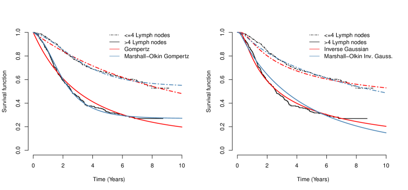
Figure 1: Estimated survival curve obtained via Kaplan-Meier estimator (black line) for colon dataset, and frequentist survival function estimates according to Gompertz regression, inverse Gaussian regression, Marshall-Olkin Gompertz regression and Marshall-Olkin inverse Gaussian regression models.

Figure 2 presents the study of case-deletion measures $GD_{i}(\bm{\vartheta})$ and $LD_{i}(\bm{\vartheta})$, which were presented in Section 1, for the Marshall-Olkin Gompertz model. For the total of 929 observations, the measures detected 7 potential influential observations: 14 ($t_{14}=7.972603$, $\delta_{14}=1$, $X_{1_{14}}=0$), 21 ($t_{21}=7.972603$, $\delta_{21}=1$, $X_{1_{21}}=0$), 116 ($t_{116}=7.641096$, $\delta_{116}=1$, $X_{1_{116}}=1$), 139 ($t_{139}=7.446575$, $\delta_{139}=1$, $X_{1_{139}}=0$), 172 ($t_{172}=7.104110$, $\delta_{172}=1$, $X_{1_{172}}=0$), 226 ($t_{228}=1.641096$, $\delta_{226}=1$, $X_{1_{226}}=0$) and 235 ($t_{235}=7.465753$, $\delta_{235}=1$, $X_{1_{235}}=0$). The majority of influential points detected from both measures has large survival time in years, with the occurence of the event of interest. On exception in an observation of group 0 (less than 4 positive lymph nodes) with survival time equal to 1.641096.

Figure 2: Index plot of $GD_{i}(\bm{\vartheta})$ and $LD_{i}(\bm{\vartheta})$ for $\bm{\vartheta}$ on the colon data set.

In order to evaluate the impact on the defective regression model of detected influential cases, we develop two relative cases (RC) measures. They are computed by excluding the influential observations detected by $GD_{i}(\bm{\vartheta})$ or $LD_{i}(\bm{\vartheta})$, and repeating the estimation process. The RC for parameters and their standard errors (SEs) are respectively given by

$$\text{RC}(\theta_{j(I_{i})})=\left|\dfrac{\hat{\theta}_{j}-\hat{\theta}_{j(I_{i})}}{\hat{\theta}_{j}}\right|\times 100\%\quad\quad\text{RC}(SE(\theta_{j(I_{i})}))=\left|\dfrac{\widehat{SE}(\hat{\theta}_{j})-\widehat{SE}(\hat{\theta}_{j})_{(I_{i})}}{\widehat{SE}(\hat{\theta}_{j})}\right|\times 100\%,$$

where $\hat{\theta}_{j(I_{i})}$ and $\widehat{SE}(\hat{\theta}_{j})_{(I_{i})}$ are the ML estimates without the $i-$th set of observations ($I_{i}$), respectively, for all $\theta_{j}\in\bm{\vartheta}$, $j=1,2,3,4,5$. The corresponding values of $\text{RC}(\theta_{j(I_{i})})$, $\text{RC}(SE(\theta_{j(I_{i})}))$, and the 95% confidence interval for parameters for 9 different dropping cases are presented in Table LABEL:tab:rc_mog. In analysis, for the majority of cases, the values of these measures are high, revealing an impact in the frequentist estimation. The statistical significance through the 95% confidence intervals is not evident for when considering the sets of dropping cases: $I_{1}=\{14\}$, $I_{2}=\{21\}$, $I_{3}=\{116\}$, $I_{4}=\{172\}$, $I_{5}=\{228\}$, $I_{6}=\{235\}$, $I_{7}=\{235\}$ and $I_{8}=\{14,21,116,139,172,228,235\}$. The most favorable scenario occurs when we drop all influential observations, when the values of $\text{RC}(\theta_{j(I_{i})})$ and $\text{RC}(SE(\theta_{j(I_{i})}))$ are small and the statistical significance remains after exclusion.

Table 9: RCs (in %) in Ml estimates and their corresponding SEs for the indicated parameter and dropped cases, and respective 95% confidence intervals for colon data.

Dropping case		$\hat{a}_{0}$	$\hat{a}_{1}$	$\hat{b}_{0}$	$\hat{b}_{1}$	$\hat{\lambda}$
{14}	RC($\hat{\bm{\vartheta}}$)	107,7488	134,8056	1378,3497	79,4254	99,9122
	RC($SE(\hat{\bm{\vartheta}})$)	28,4056	18,0945	567,8944	94,1157	99,7093
	C.I (95%)	[-0,0301 ; 0,0978]	[-0,0567 ; 0,1788]	[-8,0356 ; -3,4143]	[0,7546 ; 1,4438]	[0,0000 ; 0,1184]
{21}	RC($\hat{\bm{\vartheta}}$)	107,1138	131,313	1272,7028	79,4718	99,8593
	RC($SE(\hat{\bm{\vartheta}})$)	24,0553	32,2441	1015,3776	94,2255	99,2206
	C.I (95%)	[-0,0368 ; 0,099]	[-0,077 ; 0,1867]	[-9,1105 ; -1,3931]	[0,7547 ; 1,4443]	[0,0000 ; 0,2788]
{116}	RC($\hat{\bm{\vartheta}}$)	108,6693	129,6043	1378,7423	83,1414	99,9114
	RC($SE(\hat{\bm{\vartheta}})$)	28,7278	18,721	568,3116	94,1907	99,7067
	C.I (95%)	[-0,0258 ; 0,1016]	[-0,0665 ; 0,1703]	[-8,0388 ; -3,4146]	[0,7772 ; 1,4667]	[0,0000 ; 0,1195]
{139}	RC($\hat{\bm{\vartheta}}$)	107,3013	133,0448	1307,9833	78,7314	99,88
	RC($SE(\hat{\bm{\vartheta}})$)	27,1161	22,4484	732,1279	94,0243	99,5046
	C.I (95%)	[-0,0332 ; 0,097]	[-0,0642 ; 0,18]	[-8,2886 ; -2,531]	[0,7505 ; 1,4394]	[0,0000 ; 0,1897]
{172}	RC($\hat{\bm{\vartheta}}$)	107,6837	133,5917	1344,5848	79,7658	99,8977
	RC($SE(\hat{\bm{\vartheta}})$)	27,8237	20,3085	690,4795	94,0946	99,5988
	C.I (95%)	[-0,0309 ; 0,0981]	[-0,0611 ; 0,1788]	[-8,3084 ; -2,839]	[0,7567 ; 1,4458]	[0,0000 ; 0,1557]
{228}	RC($\hat{\bm{\vartheta}}$)	107,8193	134,6593	1377,4635	79,5317	99,9117
	RC($SE(\hat{\bm{\vartheta}})$)	28,451	18,1151	570,4407	94,1229	99,7067
	C.I (95%)	[-0,0298 ; 0,0981]	[-0,057 ; 0,1785]	[-8,0404 ; -3,4015]	[0,7552 ; 1,4444]	[0,0000 ; 0,1194]
{235}	RC($\hat{\bm{\vartheta}}$)	107,8254	134,7978	1381,378	79,4943	99,9133
	RC($SE(\hat{\bm{\vartheta}})$)	28,4941	17,9398	557,7398	94,1273	99,7174
	C.I (95%)	[-0,0297 ; 0,0981]	[-0,0566 ; 0,1786]	[-8,014 ; -3,463]	[0,755 ; 1,4442]	[0,0000 ; 0,1157]
{14, 21, 116, 172, 228, 235}	RC($\hat{\bm{\vartheta}}$)	102,7269	132,1297	1168,9944	76,2331	99,7849
	RC($SE(\hat{\bm{\vartheta}})$)	78,5597	280,9923	4218,4356	110,2445	95,3827
	C.I (95%)	[-0,1477 ; 0,1715]	[-0,3236 ; 0,4362]	[-19,7273 ; 10,1525]	[0,7064 ; 1,4529]	[0,0000 ; 1,3984]
{14, 21, 116, 139, 172, 228, 235}	RC($\hat{\bm{\vartheta}}$)	13,0082	10,5628	38,7732	10,2693	31,5898
	RC($SE(\hat{\bm{\vartheta}})$)	1,4468	1,8015	8,3273	6,0493	30,4851
	C.I (95%)	[-0,582 ; -0,4059]	[-0,2583 ; -0,0553]	[0,3043 ; 0,9386]	[0,3829 ; 0,7165]	[16,8278 ; 90,8902]

The two residual measures for the Marshall-Olkin Gompertz defective regression model using frequentist estimation in colon data set described in previous sections are shown in Figure 3. By analyzing the deviance component residual plot, we can notice a set of 5 observations as possible outliers, indicating the model is well-fitted to data.

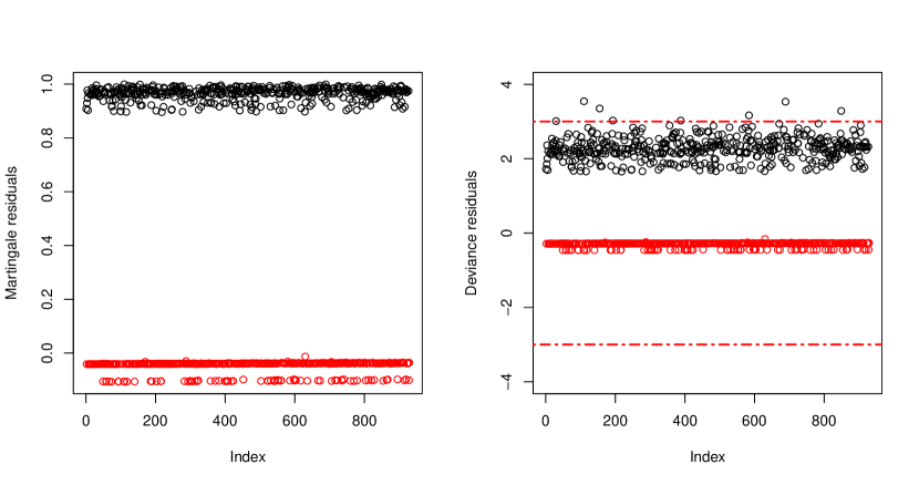
Figure 3: Index plot of the Martingale and Deviance residuals for censored (red) and non-censored (black) observations on frequentist approach for the colon data set.

4.2 Bayesian Analysis

The same analysis was conducted in colon data set under the Bayesian approach presented in Section 2.7. For the MCMC sampler, we considered the same prior distribution and set vague information to model parameters, i.e, $a_{0}\sim Normal(0,10^{2})$, $a_{1}\sim Normal(0,10^{2})$, $b_{0}\sim Normal(0,10^{2})$, $b_{1}\sim Normal(0,10^{2})$ and $\lambda\sim Gamma(0.01,0.01)$, for both Marshall-Olkin Gompertz regression and Marshall-Olkin inverse Gaussian regression. We generated one chain with 8,000 iterations and eliminated the first 2,000 ones as burn-in period. Thereby, with a total of 6,000 samples from the posterior distribution, which presented good diagnostic outcomes.

For model selection in Table LABEL:tab:model_selection_Bayes, we used the metrics LPML, WAIC and DIC criterion. Those ones have a solid theory Based on posterior predictions, which is decribes in Appendix A.2. The transformation for LPML (-2*LPLM) and WAIC (-2*WAIC) were conveniently defined to help with the same interpretation as the DIC criterion, that is, the smaller the value, the better the model fits the data used. Based on Table LABEL:tab:model_selection_Bayes, we can notice the Marshall-Olkin Gompertz regression model presents the lowest values for the three criterion metrics, indicating a more appropriate fit to colon data set.

Table 10: Values of -2*LPML, -2*WAIC and DIC for Gompertz regression, inverse Gaussian regression, Marshall-Olkin Gompertz regression and Marshall-Olkin inverse Gaussian regression models, for colon data set.

Model	-2*LPLM	-2*WAIC	DIC
Gompertz	2833.01	2833.01	2833.51
Inverse Gaussian	2863.40	2863.47	2858.16
Marshall-Olkin Gompertz	2781.08	2781.08	2779.12
Marshall-Olkin inverse Gaussian	2836.58	2836.29	2829.08

The Table LABEL:tab:Bayes_mog shows the posterior summary of Marshall-Olkin Gompertz regression, which is the best model obtained previously. The point estimation through the posterior means of each parameter are close to the values seen in Table LABEL:tab:freq_MC_MOG, which is related to the frequentest approach. The 95% credibility interval also indicates the statistical significant effect of covariate $X_{1}$ to the parameters of shape and scale of the base model. Given that both values of $a_{0}$ and $a_{1}$ estimated as negative, the model becomes defective, enabling the calculation of the cure fraction for both groups. The cure fraction for individuals with less or more than 4 positive lymph nodes in the the Bayesian Marshall-Olkin Gompertz regression are, respectively,

$$\hat{p}(X_{01})=\dfrac{\hat{\lambda}\,\hat{p}_{0}(X_{01})}{\hat{\lambda}\,\hat{p}_{0}(X_{01})+1-\hat{p}_{0}(X_{01})}=\dfrac{38.8549\,\hat{p}_{0}(X_{01})}{38.8549\,\hat{p}_{0}(X_{01})+1-\hat{p}_{0}(X_{01})}=0.5583,$$

where $\hat{p}_{0}(X_{01})=\exp\left\{\dfrac{\exp(\hat{b}_{0})}{\hat{a}_{0}}\right\}=\exp\left\{\dfrac{\exp(0.3877)}{-0.4262}\right\}=0.0315$, and

$$\hat{p}(X_{11})=\dfrac{\hat{\lambda}\,\hat{p}_{0}(X_{11})}{\hat{\lambda}\,\hat{p}_{0}(X_{11})+1-\hat{p}_{0}(X_{11})}=\dfrac{38.8549\,\hat{p}_{0}(X_{11})}{38.8549\,\hat{p}_{0}(X_{11})+1-\hat{p}_{0}(X_{11})}=0.2859,$$

where $\hat{p}_{0}(X_{11})=\exp\left\{\dfrac{\exp(\hat{b}_{0}+\hat{b}_{1})}{\hat{a}_{0}+\hat{a}_{1}}\right\}=\exp\left\{\dfrac{\exp(0.3877+0.6248)}{-0.4262-0.1742}\right\}=\exp\left\{\dfrac{\exp(1.0125)}{-0.6004}\right\}=0.0102$.

Table 11: Bayesian results of parameters estimates for Marshall-Olkin Gompertz regression for colon data set.

Parameter	Mean	SD	C.I (95%)
$a_{0}$	-0.4262	0.0454	(-0.5104 ; -0.3352)
$a_{1}$	-0.1742	0.0496	(-0.2735 ; -0.0815)
$b_{0}$	0.3877	0.1798	(0.0071 ; 0.7060)
$b_{1}$	0.6248	0.0909	(0.4594 ; 0.8184)
$\lambda$	38.8549	13.6441	(18.3463 ; 71.3956)

Additionaly, we also present the results of the Marshall-Olkin inverse Gaussian regression model in Table LABEL:tab:Bayes_moig. Similarly, the posterior means of model parameters are close to the values of MLEs estimates in Table LABEL:tab:freq_MC_MOIG, reflecting the low impact of vague information of prior distribution. The positive estimated values of $a_{0}$ and $a_{1}$ also indicate that this model does not capture the presence of cure fraction in both groups of covariate $X_{1}$.

Table 12: Bayesian results of parameters estimates for Marshall-Olkin inverse Gaussian regression for colon data set.

Parameter	Mean	SD	C.I (95%)
$a_{0}$	0.1426	0.0547	(0.0452 ; 0.2566)
$a_{1}$	0.3384	0.0640	(0.2291 ; 0.4806)
$b_{0}$	-0.2844	0.1951	(-0.6268 ; 0.1312)
$b_{1}$	0.5923	0.2059	(0.2122 ; 1.015)
$\lambda$	4.9451	1.4356	(2.8009 ; 8.2459)

In Figure 4, we present the survival curves of the two models proposed in comparison with Bayesian model fitting of their base form over the description of Kaplan-Meier curve. In the left side, the Marshall-Olkin Gompertz regression describes better the two survival curves, in contrast, the Gompertz regression does not fit well the survival curve for the individuals with more than 4 positive lymph nodes. In the right side, the both Marshal-olkin inverse gaussian and inverse Gaussian regression models does not explain properly the group of patients with with more than 4 positive lymph nodes, indicating that the base distribution and its generalization in the Marshall-Olkin family may not be appropriate for colon data. These conclusions are similar in Figure 1, which presents the survival curves under the frequentist approach.

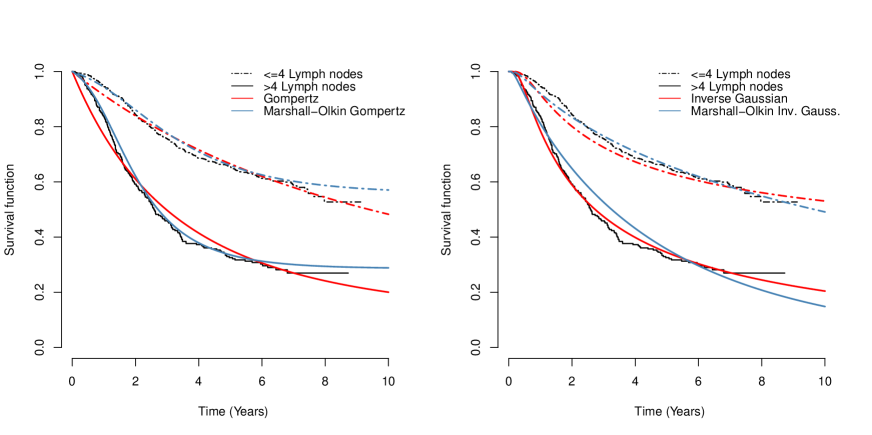
Figure 4: Estimated survival curve obtained via Kaplan-Meier estimator (black line) for colon dataset, and Bayesian survival function estimates according to Gompertz regression, inverse Gaussian regression, Marshall-Olkin Gompertz regression and Marshall-Olkin inverse Gaussian regression models.

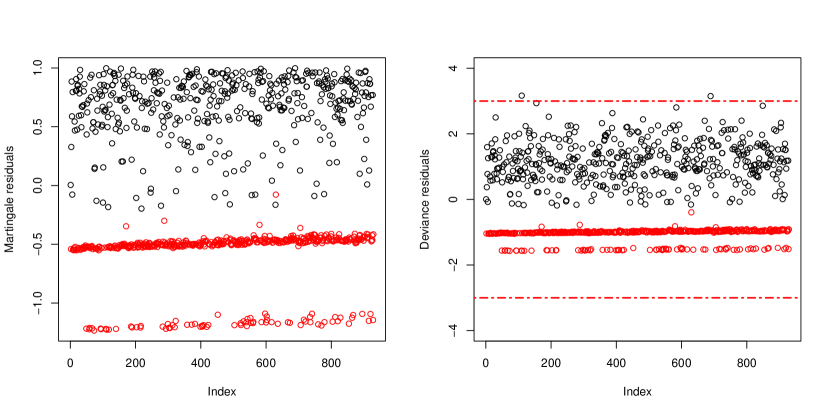
Figure 5: Index plot of the Martingale and deviance component residuals for censored (red) and non-censored (black) observations on Bayesian approach for the colon data set.

As in the classical approach, the martingale and deviance component residuals are presented in the Figure 5, evaluated on the posterior samples. The deviance component residuals indicates only two observations as possible outliers, indicating, suggesting that the Bayesian survival model is also a good fit for colon data set.

5 Conclusion

In this paper, we have proposed two new survival regression model using flexible defective distributions in the Marshall-Olkin family for long-term survival data. The regression structure were implemented in the parameters of basal cure fraction of each model with auxiliary link functions. In addition, we introduce the first estimation under Bayesian paradigm for the Marshall-Olkin Gompertz and Marshall-Olkin inverse Gaussian. Some simulations studies were designed to evaluate the asymptotic properties of maximum likelihood estimation and frequentist behaviour of posterior densities. The proposed regression models were applied to colon cancer data, which demonstrated the improvement for model-fitting in the Marshall-Olkin family and the best performance of Marshall-Olkin Gompertz regression to describe the presence of cure fraction using the quantity of positive lymph nodes of patients as covariate. The development of frailty models is strongly encouraged to capture the effect of unobserved variables for future works. We hope this work will have broad applicability in health data and other fields.

Appendix A Model selection criteria

A.1 Frequentist selection metrics

Under the frequentist estimation framework, after the estimation of the model parameters, model selection metrics aim to evaluate the value obtained from maximizing the log-likelihood function ($\ell$) in relation to the number of parameters in the statistical model ($k$). Some metrics also take into account the sample size ($n$). In general, among the various models applicable to a given dataset, the one that yields the lowest value for the selection metrics is considered the most suitable for fitting. For further details, Choi & Jeong (2019) and Bozdogan (1987) are good references.

In this paper, the following metrics were considered:

AICc $$=(-2\ell+2k)+\dfrac{2k(k+1)}{(n-k-1)},$$ (21)

BIC $$=-2\ell+k\log(n),$$ (22)

HQIC $$=-2\ell+2k\log[\log(n)],$$ (23)

CAIC $$=-2\ell+k\,[\log(n)+1],$$ (24)

where 21 is the Corrected Akaike Information Criteria (AICc), 22 is the Bayesian Information Criterion (BIC), 23 is the Hannan-Quinn Information Criterion (HQIC) and 24 is the Consistent Akaike Information Criterion (CAIC).

A.2 Bayesian selection metrics

For Bayesian statistical models, there are metrics for comparison based on posterior predictions and cross-validation. The famous ones are the logarithm of pseudo-marginal likelihood (LPML), Deviance information (DIC) and Watanabe-Akaike information (WAIC).

Let $t=(t_{1},\dots,t_{n})$ be observed survival times from a probability density function $f(.\mid\bm{\vartheta})$. The conditional predictive ordinate (CPO) estimates from the probability of observing $t_{i}$ in the future after having already observed the data $D_{[-i]}$, where $D_{[-i]}$ denotes full data excluding the $i-$th observation. We denote $\pi(\bm{\vartheta}\mid D_{[-i]})$ as the posterior density of $\bm{\vartheta}$ given $D_{[-i]}$, $i=1,2,\dots,n$. The CPO for the $i-$th observation is given by

$$\text{CPO}_{i}=\int_{\bm{\vartheta}\in\Omega}f(t_{i}\mid\bm{\vartheta})\,\pi(\bm{\vartheta}\mid D_{[-i]})\,d\bm{\vartheta}=\left\{\int_{\bm{\vartheta}}\dfrac{\pi(\bm{\vartheta}\mid D)}{f(t_{i}\mid\bm{\vartheta})}\,d\bm{\vartheta}\right\}^{-1},$$

where $t_{i}$ is the $i-$th observed survival time and $f(t_{i}\mid\bm{\vartheta})$ is the probability density function. When the analytical solution is not possible, the CPO can be estimated from MCMC samples (Ibrahim et al., 2001). By considering the inverse likelihood across $S$ iterations, the CPO for the $i-$th observation can be computed as

$$\widehat{\text{CPO}}_{i}=\left(\dfrac{1}{S}\sum^{S}_{s=1}\dfrac{1}{f(t_{i}\mid\bm{\vartheta}_{s})}\right)^{-1}.$$

To take account the information of CPO computed in each observation, the logarithm of the pseudomarginal likelihood (LPLM) is defined as

$$\text{LPML}=\sum^{n}_{i=1}\log(\widehat{\text{CPO}}_{i}).$$

The model with larger value of LPML is preferred for model-fitting.

The Deviance Criterion Information (DIC) is another measure to compare Bayesian models, which penalizes the model fitting based on complexity (Spiegelhalter et al., 2002). The deviance has the following expression

$$D(\bm{\vartheta})=-2\sum_{i=1}^{n}\log\left(f(t_{i}\mid\bm{\vartheta})\right),$$

where $f(.)$ is the corresponding probability density function of model under evaluation. The posterior mean of $D(\bm{\vartheta})$ can be obtained by from posterior samples. In fact, $\overline{D}=\sum_{s=1}^{S}D(\bm{\vartheta}^{s})$, where $\bm{\vartheta}^{s}$ is the $s-$th posterior sample. Spiegelhalter et al. (2002) recommend the estimation of DIC as

$$\widehat{\text{DIC}}=\overline{D}+0.5\,p_{D},$$

where $p_{D}$ is the effective parameters numbers, estimated via

$$\widehat{\text{Var}}(D(\bm{\vartheta}))=\dfrac{1}{S-1}\sum^{S}_{s=1}[D(\bm{\vartheta})^{s}-\overline{D}]^{2}.$$

Under these definitions, the smaller value of DIC indicates the best model for data.

Watanabe Akaike’s information (WAIC) proposed by Watanabe & Opper (2010) is another criterion for model selection. The method is based on the logarithm of predictive density (lpd), given by

lpd $$=\sum_{i=1}^{n}\log\left(p_{post}(t_{i})\right)$$

$$=\sum_{i=1}^{n}\log\left(\int_{\bm{\vartheta}\in\Omega}f(t_{i}\mid\bm{\vartheta})\,\pi(\bm{\vartheta}\mid D)\,d\bm{\vartheta},\right),$$ (25)

In practice, the lpd can be calculated using the posterior samples obtained from $\pi(\bm{\vartheta}\mid D)$. In this sense,

$$\widehat{lpd}=\sum_{i=1}^{n}\log\left(\dfrac{1}{S}\sum_{s=1}^{S}f(t_{i}\mid\bm{\vartheta}^{(s)})\right),$$

where $f(t_{i}\mid\bm{\vartheta}^{(s)})$ represents the data observed density function evaluated by the $s-$ posterior sample.

We also need to define the correspondent bias correction (pd) for the effective number of parameters to avoid overfitting,

$$pd=\sum^{n}_{i=1}\log\left(\int_{\bm{\vartheta}\in\Omega}f(y_{i}\mid\bm{\vartheta})\,\pi(\bm{\vartheta}\mid D)\,d\bm{\vartheta}\right)-\int_{\bm{\vartheta}\in\Omega}\log\left(f(y_{i}\mid\bm{\vartheta})\right)\,\pi(\bm{\vartheta}\mid D)\,d\bm{\vartheta},$$

which can be estimated from posterior samples as

$$\widehat{pd}=2\sum^{n}_{i=1}\left(\log\left(\dfrac{1}{S}\sum_{s=1}^{S}f(t_{i}\mid\bm{\vartheta}^{s})\right)-\dfrac{1}{S}\sum^{S}_{s=1}\log\left(f(t_{i}\mid\bm{\vartheta}^{s})\right)\right).$$

The WAIC is given by

$$\widehat{WAIC}=\widehat{lpd}-\widehat{pd}.$$

Large values of WAIC computed on Bayesian model indicates a better fit for data. To facilitate the interpreattion of all results (in the same scale), we multiply the LPML and WAIC values by $-2$, respectively.

References

- (1)
- Barreto-Souza et al. (2013) Barreto-Souza, W., Lemonte, A. J. & Cordeiro, G. M. (2013), ‘General results for the marshall and olkin’s family of distributions’, Anais da Academia Brasileira de Ciências 85(1), 3–21.
- Berkson & Gage (1952) Berkson, J. & Gage, R. P. (1952), ‘Survival curve for cancer patients following treatment’, Journal of the American Statistical Association 47(259), 501–515.
- Boag (1949) Boag, J. W. (1949), ‘Maximum likelihood estimates of the proportion of patients cured by cancer therapy’, Journal of the Royal Statistical Society. Series B (Methodological) 11(1), 15–53.
- Bozdogan (1987) Bozdogan, H. (1987), ‘Model selection and akaike’s information criterion (aic): The general theory and its analytical extensions’, Psychometrika 52(3), 345–370.
- Burda & Maheu (2013) Burda, M. & Maheu, J. M. (2013), ‘Bayesian adaptively updated hamiltonian monte carlo with an application to high-dimensional bekk garch models’, Studies in nonlinear dynamics and econometrics 17(4), 345–372.
- Calsavara et al. (2019) Calsavara, V. F., Rodrigues, A. S., Rocha, R., Tomazella, V. & Louzada, F. (2019), ‘Defective regression models for cure rate modeling with interval-censored data’, Biometrical Journal 61(4), 841–859.
- Choi & Jeong (2019) Choi, I. & Jeong, H. (2019), ‘Model selection for factor analysis: Some new criteria and performance comparisons’, Econometric Reviews 38(6), 577–596.
- Colosimo & Giolo (2021) Colosimo, E. A. & Giolo, S. R. (2021), Análise de sobrevivência aplicada, Editora Blucher.
- Gieser et al. (1998) Gieser, P. W., Chang, M. N., Rao, P., Shuster, J. J. & Pullen, J. (1998), ‘Modelling cure rates using the gompertz model with covariate information’, Statistics in medicine 17(8), 831–839.
- Huang et al. (2021) Huang, J., Yu, S., Ding, L., Ma, L., Chen, H., Zhou, H., Zou, Y., Yu, M., Lin, J. & Cui, Q. (2021), ‘The dual role of circular rnas as mirna sponges in breast cancer and colon cancer’, Biomedicines 9(11), 1590.
- Ibrahim et al. (2001) Ibrahim, J. G., Chen, M.-H., Sinha, D., Ibrahim, J. & Chen, M. (2001), Bayesian survival analysis, Vol. 2, Springer.
- Le Voyer et al. (2003) Le Voyer, T., Sigurdson, E., Hanlon, A., Mayer, R., Macdonald, J., Catalano, P. & Haller, D. (2003), ‘Colon cancer survival is associated with increasing number of lymph nodes analyzed: a secondary survey of intergroup trial int-0089’, Journal of clinical oncology 21(15), 2912–2919.
- Lin & Zhu (2008) Lin, J. & Zhu, H. (2008), A cure rate model in reliability for complex system, in ‘2008 IEEE International Conference on Industrial Engineering and Engineering Management’, IEEE, pp. 1395–1399.
- Maller & Zhou (1996) Maller, R. A. & Zhou, X. (1996), ‘Survival analysis with long-term survivors’, (No Title) .
- Marshall & Olkin (1997) Marshall, A. W. & Olkin, I. (1997), ‘A new method for adding a parameter to a family of distributions with application to the exponential and weibull families’, Biometrika 84(3), 641–652.
- Martinez & Achcar (2017) Martinez, E. Z. & Achcar, J. A. (2017), ‘The defective generalized gompertz distribution and its use in the analysis of lifetime data in presence of cure fraction, censored data and covariates’, Electronic Journal of Applied Statistical Analysis 10(2), 463–484.
- Martinez & Achcar (2018) Martinez, E. Z. & Achcar, J. A. (2018), ‘A new straightforward defective distribution for survival analysis in the presence of a cure fraction’, Journal of Statistical Theory and Practice 12(4), 688–703.
- Paulino et al. (2018) Paulino, C. D. M., Turkman, M. A. A. & Murteira, B. (2018), Estatística bayesiana.
-
Plummer et al. (2006)
Plummer, M., Best, N., Cowles, K. & Vines, K. (2006), ‘Coda: Convergence diagnosis and output analysis for mcmc’, R News 6(1), 7–11.
https://journal.r-project.org/archive/ -
R Core Team (2023)
R Core Team (2023), R: A Language and Environment for Statistical Computing, R Foundation for Statistical Computing, Vienna, Austria.
https://www.R-project.org/ -
R Core Team (2024)
R Core Team (2024), R: A Language and Environment for Statistical Computing, R Foundation for Statistical Computing, Vienna, Austria.
https://www.R-project.org/ - Rocha (2016) Rocha, R. F. d. (2016), ‘Defective models for cure rate modeling’.
- Rocha et al. (2016) Rocha, R., Nadarajah, S., Tomazella, V. & Louzada, F. (2016), ‘Two new defective distributions based on the marshall–olkin extension’, Lifetime data analysis 22, 216–240.
- Rodrigues et al. (2009) Rodrigues, J., Cancho, V. G., de Castro, M. & Louzada-Neto, F. (2009), ‘On the unification of long-term survival models’, Statistics & Probability Letters 79(6), 753–759.
- Rodrigues (2020) Rodrigues, J. S. (2020), ‘Cure rate models: alternatives methods to estimate the cure rate’.
- Sigurdson (2003) Sigurdson, E. R. (2003), ‘Lymph node dissection: is it diagnostic or therapeutic?’.
- Spiegelhalter et al. (2002) Spiegelhalter, D. J., Best, N. G., Carlin, B. P. & Van Der Linde, A. (2002), ‘Bayesian measures of model complexity and fit’, Journal of the royal statistical society: Series b (statistical methodology) 64(4), 583–639.
-
Stan Development Team (2024)
Stan Development Team (2024), ‘RStan: the R interface to Stan’.
R package version 2.35.0.9000.
https://mc-stan.org/ - Tepper et al. (2001) Tepper, J. E., O’connell, M. J., Niedzwiecki, D., Hollis, D., Compton, C., Benson III, A. B., Cummings, B., Gunderson, L., Macdonald, J. S. & Mayer, R. J. (2001), ‘Impact of number of nodes retrieved on outcome in patients with rectal cancer’, Journal of clinical oncology 19(1), 157–163.
-
Therneau (2024)
Therneau, T. M. (2024), A Package for Survival Analysis in R.
R package version 3.7-0.
https://CRAN.R-project.org/package=survival - Therneau et al. (1990) Therneau, T. M., Grambsch, P. M. & Fleming, T. R. (1990), ‘Martingale-based residuals for survival models’, Biometrika 77(1), 147–160.
- Tsodikov et al. (1996) Tsodikov, A. D., Yakovlev, A. Y. & Asselain, B. (1996), Stochastic models of tumor latency and their biostatistical applications, Vol. 1, World Scientific.
- Watanabe & Opper (2010) Watanabe, S. & Opper, M. (2010), ‘Asymptotic equivalence of bayes cross validation and widely applicable information criterion in singular learning theory.’, Journal of machine learning research 11(12).