Learning Mean First Passage Time: Chemical Short-Range Order and Kinetics of Diffusive Relaxation
Abstract
Long-timescale processes pose significant challenges in atomistic simulations, particularly for phenomena such as diffusion and phase transitions. We present a deep reinforcement learning (DRL)-based computational framework, combined with a temporal difference (TD) learning method, to simulate long-timescale atomic processes of diffusive relaxation. We apply it to study the emergence of chemical short-range order (SRO) in medium- and high-entropy alloys (MEAs/HEAs), which plays a crucial role in unlocking unique material properties, and find that the proposed method effectively maps the relationship between time, temperature, and SRO change. By accelerating both the sampling of lower-energy states and the simulation of transition kinetics, we identify the thermodynamic limit and the role of kinetic trapping in the SRO. Furthermore, learning the mean first passage time to a given, target SRO relaxation allows capturing realistic timescales in diffusive atomistic rearrangements. This method offers valuable guidelines for optimizing material processing and extends atomistic simulations to previously inaccessible timescales, facilitating the study of slow, thermally activated processes essential for understanding and engineering material properties.
I Introduction
Atomistic simulations have long been confronted with challenges to capture physical phenomena that occur over extended timescales due to inherent computational limitations [1]. Many critical material processes, such as phase transitions and mechanical deformation span a wide range of timescales up to seconds or longer, whereas conventional molecular dynamics (MD) simulations operate within nanoseconds to microseconds [2]. This disparity becomes particularly problematic when the configurational transition rates are exponentially dependent on temperature. To overcome these challenges, advanced simulation techniques have been introduced. Machine learning interatomic potentials (ML-IPs) can accelerate the simulation by providing fast energy and forces calculations, which significantly scale up the simulation size in terms of length [3, 4, 5] compared to ab initio MD. However, they still require small integration time steps to ensure simulation stability. Utilizing transition-state theory (TST), one can accelerate MD and facilitate the sampling of rare events by hyperdynamics [6, 7], off-lattice kinetic Monte Carlo method [8], parallel replica dynamics [9], or diffusive molecular dynamics [10, 11]. Nonetheless, long-timescale simulations of processes consisting of a large number of atomic diffusion events is still a challenging task [2, 12]. Recently, we introduced the use of deep reinforcement learning (DRL) in long-timescale atomistic simulation of diffusion [13]. In this approach, the DRL agent can function as an accelerated KMC simulator for transition kinetics and as a Monte Carlo (MC) sampler for free-energy minimization, corresponding to a transition kinetics simulator (TKS) and lower-energy states sampler (LSS), respectively. One may consider DRL-LSS to be computationally efficient option for reaching thermodynamic equilibrium, while DRL-TKS option to be faithful to the true timescale of kinetics, of say approaching that equilibrium after some external condition sustains a step change, e.g. relaxation.
One particular application where long-timescale phenomena are critical is in the study of chemical short-range order (SRO) in multi-principal-component medium- and high-entropy alloys (MEAs/HEAs) [14, 15, 16, 17]. These alloys have gained significant attention due to their superior mechanical, physical or catalytic properties compared to conventional metal alloys that typically consist of one or two principal components of compositions [18, 19, 20, 21, 22]. The evolution of SRO can have significant effects on applied materials properties, such as mechanical and magnetic properties [23, 24, 25, 26]. The process of inducing SRO in MEAs/HEAs often involves thermal annealing from an elevated temperature [14]. This introduces an engineering degree of freedom to tailor material properties, as SRO does not necessarily correspond to the equilibrium states but depends on the parameters during the material processing.
Understanding the processing-structure-properties relation of MEAs/HEAs is not a trivial task, mainly because experimental quantification of the nanometer scale features of the SRO is very challenging and the formation of SRO is very sensitive to the processing conditions. ML-accelerated simulations have been applied to a number of related tasks in MEAs/HEA. Recently, the Freitas group has developed a ML-IP for CrCoNi and successfully identified the thermodynamic equilibrium atomic configurations via ML-IP accelerated Monte Carlo (MC) sampling as a function of temperature, providing various metrics for SRO [24, 27]. Conventional sampling algorithm of MC for thermal equilibrium states generally do not consider the physical transition of atomic configurations and thus do not provide kinetic information along the evolution trajectory. The Ogata group has demonstrated a machine learning accelerated kinetic Monte Carlo (KMC) simulation of vacancy diffusion in CrCoNi to investigate the SRO formation kinetics [28, 29, 30]. Nevertheless, obtaining a complete transition trajectory to the equilibrium state is nearly unattainable in KMC at lower temperatures, such as room temperature (RT), which is often the application temperature, because of the extensive sampling needed.
In this work, we tackle the long-timescale challenge by employing deep reinforcement learning (DRL) and learning the mean first passage time (MFPT), the time required for an atomic arrangement to evolve toward thermodynamic equilibrium states. We investigate the single-phase transition of atomic ordering with the acquisition of vacancy-mediated SRO formation in CrCoNi. An equivariant graph neural network (GNN) is used to encode vacancy diffusion reactions and predict the kinetic and thermodynamic parameters of these events. The DRL framework enables the successful tracking of SRO formation trajectories at varying temperatures. In addition, we propose a temporal difference (TD) learning scheme to train a time estimator for predicting the MFPT. The time estimator addresses the lack of kinetic information along thermodynamic trajectories of SRO formation. By simulating SRO formation for different annealing temperatures and vacancy concentrations (), we successfully map the correlation between SRO, time, temperature, and . This provides valuable insights and guidelines for optimizing materials processing to achieve desired SROs. Moreover, our method overcomes the timescale limitations of conventional atomistic simulations, extending its applicability to a wide range of long-timescale transformations.
II Results and discussion
II.1 General computational framework
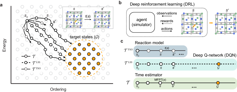
Figure 1 provides an overview of our computational framework for simulating long-timescale processes using the example of vacancy-mediated SRO formation in equiatomic CrCoNi during thermal annealing. In the potential energy landscape of CrCoNi, a potential energy local minimum is denoted as a state , which corresponds to a specific arrangement of atoms and vacancies in the face-centered cubic (fcc) lattice sites. From a given state , multiple atomic transitions involving vacancy diffusion to adjacent states can occur. In this work, we define a mono-vacancy diffusion to a neighboring atomic site as an action, denoted by . Each action corresponds to a transition rate, , whose rate can be evaluated by the transition-state theory [31]:
| (1) |
where and are the energy barrier and attempt frequency of transition from to , respectively. The average stationary time of the system in state can then be defined as:
| (2) |
The set of all possible actions starting from constitutes the action space, , and the collection of all possible states defines the state space . Under annealing conditions at a given temperature, CrCoNi evolves into certain orderings of atomic configurations that, in the time limit, minimize the free energy. Thermodynamic equilibrium of SRO () may be attained from this relaxation process if one waits for “enough” transitions under a constant temperature. We define the states corresponding to thermal equilibrium as the “target states” (). The reason for using a set of states to define thermodynamic equilibrium, instead of a single state, is because at finite temperature, there are equilibrium fluctuations, as clearly indicated by the equilibrium fluctuation-dissipation theorem, which is of the magnitude on a per-atom basis, where is the number of atoms. Thus, the “volume” in phase space is finite, as indicated in Figure 1a.
In a physical process, a series of consecutive states forms a trajectory :
| (3) |
where is an initial atomic structure such as a completely random solid solution (RSS) state and is the time horizon of the trajectory to reach the hypersurface of . It is possible to understand the kinetics along the evolution trajectory of SRO formation during the thermal annealing process, if one simulates a sufficiently long evolution trajectory that covers the whole process of SRO relaxation. However, the SRO formation process may occur at macroscopic timescales at low temperatures, making direct kinetics simulations difficult. Thus, we adopt an alternative approach using the mean first passage time (MFPT) to study the long-timescale processes.
To estimate the transformation time of SRO formation toward the , we define the MFPT as an average time of trajectories () that reach the , expressed as follows:
| (4) | ||||
Here, is a set of first passage trajectories that begin from and first enter the at its last state . The average total time for each trajectory, is given by:
| (5) |
The total probability is the product of the individual transition probabilities, where each transition probability from state to is defined as:
| (6) |
It is apparent that the MFPT equals zero if . Assuming ergodicity of the kinetic system, that means , as all trajectories enter at least once if . However, obtaining the complete trajectory with kinetic information is a very challenging task.
Figure 1b and c demonstrate how complete trajectories are obtained in our framework. In the DRL for atomic transitions, an agent (simulator) is trained to interact with an atomic system to learn optimal transitions (actions) based on an objective function (reward) aimed at either energy minimization or achieving faster transition rates. As a result, we can generate kinetic transition trajectories () and energy minimization trajectories () using the TKS and LSS, respectively. However, each separately has incomplete information. The governed by transition probabilities of vacancy hopping event explores the potential energy landscape by randomly navigating the local minima. This randomness makes it difficult to reach the as the trajectory is spread over vast high-dimensional configurational space. The is driven by the thermodynamic driving force of energy minimization. The DRL-driven LSS accelerates the convergence to and provides the correct structural evolution direction toward . However, it no longer follows the individual physical transition probabilities and loses information on real physical evolution timescale, which is an important aspect of materials kinetics. Accordingly, we re-evaluate the evolution timescale by training a machine learning surrogate model that directly predicts the MFPT.
Figure 1c shows the machine learning models used to construct different trajectories of SRO formation. Using an atomic structure and its transition to , denoted as (, ), as inputs, we developed a reaction model, a deep Q-network model, and a time estimator. The reaction model is used to generate the by predicting the energy barrier and attempt frequency of vacancy hopping event without an explicit transition state calculation. Next, we train the DQN to obtain the that provides accelerated SRO formation processes. Finally, we introduce a machine learning model of time estimator that provides the kinetic information along the , forming a complete and bridging the gap between thermodynamic equilibrium states and their physical evolution over time.
II.2 Graph neural network based reaction encoding
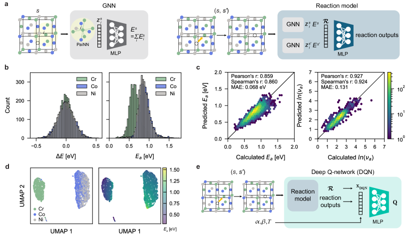
We successfully encode atomic structures and vacancy diffusion reactions with the GNN (Figure 2a). GNNs are widely used to represent atomic structures, where atoms serve as nodes and connections between neighboring atoms as edges. The GNNs, trained with available property labels, automatically learn the relationship between local chemical environments around atoms and materials or atomic properties. In this work, the GNN is designed to learn a representation for each atom () based on the total energy () of the system. For the message-passing architecture, we employ the polarizable atom interaction neural network (PaiNN) model [32], which ensures rotational equivariance for vector features inside the model layers.
To encode the diffusion reaction from a reactant to a product chemical environment, we adopt a similar approach as described in previous studies [33, 34], where the difference between the learned representation vectors of two states, and , is used for encoding the transition (, ). The GNN model is first trained on a simpler task: predicting the total energies of states . In this task, the GNN also outputs a representation vector on each node denoted as ( is the index of the node). Then, the is used to predict our target learning task, predicting transition parameters. The differences between the atomic representations of and are then computed to generate atomic difference features. These features, along with the predicted energy difference by the GNN (), are aggregated into a reaction encoding vector (), as defined in Eq. (7):
| (7) |
where SumPool is the sum pooling operation among all nodes . The reaction encoding vector is then used to predict key reaction outputs, including the energy change of the transition event (after relaxation) , activation energy (), and attempt frequency () for a given vacancy diffusion. To calculate the “ground truth” total energy of the system as well as and for vacancy diffusion, we utilize a universal ML-IP, MACE-MP-0 [35]. Details on the dataset creation and training process of the reaction model for CrCoNi vacancy diffusion are explained in Sec. IV.1.
Figures 2b and S1 depict the distribution of reaction labels. The reaction energies exhibit a unimodal distribution centered around zero for all elements. Interestingly, activation energies for vacancy diffusion to Cr sites are notably lower compared to those for Co and Ni sites. This suggests that Cr is generally more mobile than Co and Ni in vacancy-exchange diffusion events, and the SRO formation kinetics can be tuned by varying the Cr concentration, as it facilitates vacancy diffusion. On the other hand, the thermodynamic equilibrium of SRO may not depend much on vacancy concentration because is dilute (typically less than 0.1 at%). In other words, unlike the major alloying elements like , which are both thermodynamically and kinetically important, it is generally well accepted and understood that while may be key for kinetics following the Kirkendall-Smigelskas experiment in 1947, it can often be ignored for the thermodynamic equilibrium properties.
The GNN-based reaction model shows better predictive accuracy of reaction labels on the vacancy diffusion in CrCoNi than the previous model, as shown in Fig. 2c. More details and comparisons with the previous model are provided in Sec. SA of the Supplementary Information. Furthermore, the learned , effectively captures information about the impact of local environments on diffusion. Figure 2d shows 2D projections of the by the Uniform Manifold Approximation and Projection (UMAP) algorithm [36] for atomic sites of vacancy diffusion in CrCoNi. The 2D projections reveal three distinct clusters, with Co and Ni generally residing in the same cluster, while Cr forms a separate cluster. Nevertheless, distinguishes between Co and Ni within the same cluster. The color-coding of the activation energies aligns with their distribution, highlighting the lower activation energies for Cr compared to Co and Ni sites.
The GNN-based approach, which automatically learns from both structural and reaction inputs, offers distinct advantages. By using atomic feature differences for input parametrization, the model can be more easily generalized. Since vacancy diffusion during SRO formation is highly localized, atoms distant from the diffusion event exhibit minimal changes in their local environments, resulting in near-zero atomic difference features for these atoms. This locality enables the reaction model to scale up to larger cells efficiently as long as the focus remains on local events. Additionally, the reaction model can be trained to encode structures and reactions, providing a warm start (a good pre-trained representation) for the DRL framework, thereby improving training efficiency and convergence.
To build on these advantages, we employ the pre-trained reaction model within a DRL framework to simulate the formation of SRO in CrCoNi. The architecture of deep Q-network (DQN) model, which forms the core of the DRL framework, is illustrated in Fig. 2e and is discussed in detail in the following section.
II.3 Deep reinforcement learning and short-range order formation
The DQN is trained by optimizing the quality function , and is used to formulate a policy () based on Boltzmann distribution of to account for the temperature effect. Since actions are taken based on probabilities, the system’s evolution is non-deterministic. The is trained by maximizing the total reward (), which is the accumulated reward () with a discount factor, , as defined in Eq.(8) and (9):
| (8) |
The reward function, , is a sum of the kinetic () and thermodynamic () contributions, weighted by coefficients and :
| (9) |
where is the activation energy, is the reaction energy, and is the attempt frequency, with being the temperature and the Boltzmann constant.
As shown in Fig. 2e, we design the DQN to predict the for a given transition. In a transition, an action is applied to the current state and moves the system to the next state . Here, we do not relax the state for computational convenience. We first pre-train the reaction model to predict reaction outputs, by learning rich encodings for pairs of reactant-product states, provide a warm-start for DQN training. The DQN feature vector () is formulated as in Eq. (10).
| (10) | |||
We use as the input to the neural network to predict :
| (11) |
where MLPθ represents a multi-layer perceptron. The DQN model parameters are updated according to the Bellman optimality equation [37]:
| (12) |
Here, is a target network that updates less frequently, and is the learning rate. This formulation accounts for both thermodynamic and kinetic driving forces, as well as future rewards, thereby accelerating the simulation process [13]. Yet, for certain conditions of interest we can use a simplified version. If we focus solely on the instantaneous kinetic reward, setting and , the DRL framework is used as the TKS. Here, directly using the reaction model is sufficient. If we set and , we consider future rewards but atomic structure changes are only driven by the energy minimization. Thus, the DRL framework is used as the LSS. Note that the output of the DQN does not have a direct physical meaning but rather represents the quality of the chosen action for maximizing rewards.
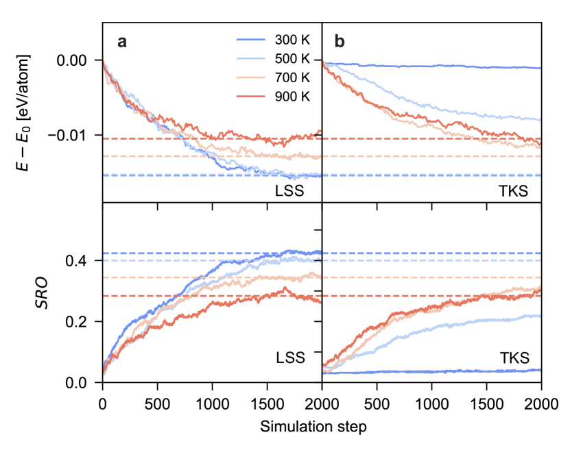
The DRL framework for SRO transformation reveals the temperature-dependent thermodynamic limits of SRO. Figure 3 shows the SRO formation in CrCoNi with a 0.39 at% of vacancy concentration across various temperatures. For LSS, lower temperatures result in lower-energy states and larger SRO, consistent with the previous results at thermal equilibrium [27]. In contrast, TKS leads to higher-energy states and smaller SRO at lower temperatures. This suggests that TKS for the SRO formation in CrCoNi is undercoverged with respect to the thermodynamic limit, because it requires a long-timescale simulation and is prone to kinetic trapping at lower temperatures, preventing the system from reaching the thermodynamic limits due to the high activation energy ( = 0.8 eV). At sufficiently high temperatures (e.g., 900 K), both LSS and TKS converge to similar states in terms of both energy and SRO. These results suggest that kinetic simulations at low temperatures can hardly capture the disorder-to-order transition, as the physical transformation time exceeds the timescale capacity of the simulation.
To further investigate the thermodynamic limits of SRO in CrCoNi, we deployed LSS with varying concentrations, as shown in Fig. S6. Our results show that the converged SRO parameters are insensitive to except at 300 K, and a slightly larger SRO appears at higher vacancy concentrations. The slight difference in equilibrium can be attributed to the volumetric strain of vacancies that changes the relative interaction energies between neighboring atoms. Note that limited by the computationally accessible supercell size, the vacancy concentrations in our simulation are set in the range of approximately to at%. Although the is much lower in most experiments, our simulation results still provide key parameters that can be extrapolated to the dilute vacancy limit in experimental conditions. When , the SRO parameters converge to a constant, and the timescale is proportional to , providing a reliable extrapolation scheme to arbitrary small .
The thermodynamic limits of SRO parameters, denoted as , are set as references of the target states in the following MFPT evaluation. To make cover the equilibrium SRO of different in our calculations, we define as configurations that have the SRO parameters () of the highest case in our simulations within a threshold (). Figure S7 shows these limits, which are considered as the center of across different temperatures. More details of the in SRO formation are explained in Sec. SB of the Supporting Information.
II.4 Time estimation
As introduced in the Sec. II.1, we aim to estimate MFPT at any intermediate state along the . In principle, the MFPT can be evaluated by directly sampling by its definition Eq. (4). However, obtaining one data point of requires sampling the entire trajectory, which is computationally expensive. In addition, the trajectory property has large variance, making the MFPT evaluation data inefficient. Therefore, we adopt a Temporal Difference (TD) learning method in reinforcement learning to train the time estimator.
We use the following Bellman equation in the TD learning:
| (13) |
Note that Eq. (13) is a self-consistent equation: given an initial MFPT, one can evaluate the right-hand side of the equation and obtain a new MFPT. Such updates of MFPT can be done iteratively until convergence. In principle, MFPT() can be updated by sampling a transition from to as shown in Eq. (14).
| (14) | |||
where equals one when is not in and zero otherwise. However, such iteration does not necessarily guarantee convergence. According to proposition 4.4. in Ref. [38], the convergence of the iteration requires the max norm contraction of the update to MFPT, which can be realized with a discount factor on the right-hand side. Therefore, we introduce a characteristic decay time for modified MFPT, denoted as . MFPTτ() is then approximated by the time estimator, . More details on the and the optimization of the time estimator are explained in Sec. IV.2.
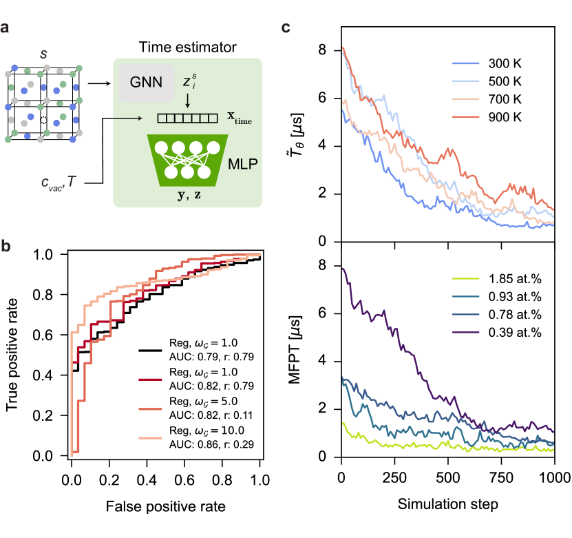
We use a multitask learning approach for the time estimator to predict MFPT of and determine whether belongs to more efficiently. Figure 4a illustrates the model architecture, where an atomic structure is encoded by the GNN and time feature vector () is formulated as follows:
| (15) |
We utilize for two tasks: one for regression to predict the time (), and the other for binary classification to produce logits (), determining whether belongs to . Then the model output, , is computed as:
| (16) |
where is the sigmoid function applied to the logits. To consider the temperature and vacancy concentration dependence of the time, we further introduce a scaler function, , for the final time output . In the training process, both tasks are included in the total loss function (see details in section IV.2. The multitask learning strategy outperforms simple regression for time estimation. Figure 4b shows the test set performance with receiver operating characteristic (ROC) curves for different time estimation models. Here, a true positive indicates that the model correctly predicts that is not in . The area under the curve (AUC) quantifies the overall accuracy at various classification thresholds, with higher AUC values indicating better binary classification accuracy. While the combined model (Reg+Cls) outperforms the regression-only model (Reg) in distinguishing , it shows a decrease in Pearson’s r for time prediction as increases. Based on these observations, Reg+Cls with set to 1.0 is selected for deployment, balancing both classification accuracy and time prediction performance.
The time estimator reveals the annealing time of the disorder-to-order transition of CrCoNi, as shown in Figure 4c and S9. At a fixed vacancy concentration of 0.39 at%, the time estimator correctly predicts the decreasing trend of along the SRO formation trajectory at various temperatures. The results show successful learning of the phase transformation dynamics as a function of temperature. The trends across different temperatures suggest that while the structural transformation is consistent, the transition kinetics vary, with faster kinetics at higher temperatures. At 500 K, a higher vacancy concentration leads to a smaller MFPT, signifying accelerated transformation kinetics due to enhanced atomic mobility. This demonstrates the crucial role of vacancies in inducing diffusion degrees of freedom and facilitating faster ordering. Overall, the time estimator effectively captures the interplay between temperature, vacancy concentration, and kinetics during SRO formation.
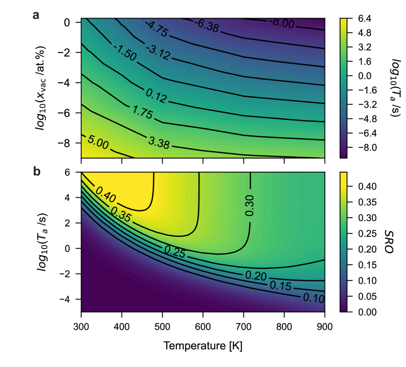
The time estimator effectively complements the thermodynamic trajectory of SRO formation at various temperatures and vacancy concentrations by providing kinetic insights of annealing time (), aiding in understanding of materials processing. We assess the process-structure-SRO relationship in two cases: one is for the SRO formation time (the evolution time from RSS to the ), and the other is for the time-dependent SRO evolution at a given vacancy concentration. Further details on how these insights are obtained are provided in Sec. SC of the Supporting Information. Figure 5a illustrates how temperature and vacancy concentration influence the annealing time to reach . Higher temperatures and increased reduce the time needed to achieve . We consider the annealing process with rapid cooling from near melting temperature of 1500 K [29] so that the vacancy concentration can be evaluated as follows:
| (17) |
where is the number of components and =1.78 eV is an average vacancy formation energies taken from the literature [29]. Under this and temperatures above 700 K, the system quickly reaches (within seconds) due to enhanced atomic mobility. At lower temperatures (300–500 K), annealing time increases exponentially with decreasing temperature, and achieving may take several days. As and annealing temperature can be controlled in experiments, the corresponding SRO formation time can then be estimated by the data presented in Fig. 5a.
Figure 5b demonstrates how temperature and annealing time impact SRO formation in CrCoNi at . The results qualitatively align with previous findings [29], showing that while longer annealing times can enhance SRO, temperature dictates the thermodynamic limits. Notably, our method enables mapping at much lower temperatures than those accessible through previous KMC simulations by integrating the equilibrated SRO formation trajectory from the LSS with the time estimator model. Tuning temperature is more efficient in the high-temperature region, whereas adjusting annealing time at a fixed temperature is more practical in the low-temperature region. Therefore, selecting both annealing temperature and time with precision is crucial to achieving the desired SRO, balancing the need for rapid kinetics at high temperatures with a more gradual ordering process at lower temperatures.
III Conclusion and Outlook
We presented a novel deep reinforcement learning (DRL)-based framework for atomistic simulation, integrated with temporal difference (TD) learning, to develop a time estimator for investigating the chemical short-range order (SRO) formation kinetics in CrCoNi medium-entropy alloy. This approach successfully captured the interplay between temperature, time, and vacancy concentration, providing key insights into the annealing process of SRO formation. Our findings demonstrate that while high temperatures promote rapid SRO formation, lower temperatures—despite providing more atomic ordering—pose high kinetic barriers that prevent the system from achieving full chemical order within practical time frames. The generated time-temperature-SRO map highlights the potential for optimizing SRO formation through tailored annealing strategies, enabling precise control over material properties in CrCoNi and other medium- and high-entropy alloys. By efficiently navigating the kinetics of phase transformations at the atomic level, this method could have far-reaching implications for designing next-generation materials with tailored mechanical, magnetic, and thermal properties. This approach provides a powerful tool for overcoming timescale limitations in atomistic simulations, offering a new pathway to engineer advanced materials with optimized microstructures.
IV Methods
IV.1 Reaction model
To pre-train the reaction model, we constructed model systems of CrCoNi consisting of 108, 256, and 500 atoms with equiatomic composition of Cr, Co, and Ni, and each with varying vacancy concentrations from 1 to 4 atomic defects. The pre-training dataset included configuration changes with labels for the total energy of two states, and , denoted as and , as well as activation energy () and attempt frequency (). The was calculated as the energy difference between the transition state, and the initial state, . The was determined using harmonic transition-state theory (HTST) [39, 13]. The transition state structure () was obtained using Nudged-Elastic Band (NEB) method [40, 41], as implemented in the Atomistic Simulation Environment (ASE) [42]. Starting from a random solid solution (RSS), we randomly sampled vacancy hopping events to generate transition data. The total dataset comprised 8,911 samples for training, with an in-distribution test set of 4,389 samples. The out-of-distribution test set included 627 samples from systems with 864 atoms, to evaluate the model’s generalizability beyond its training domain. The training loss function is defined below:
| (18) |
where is the loss for the predicted energy difference between states, , is the loss for the activation energy, is the loss for the natural logarithm of the attempt frequency, and and are the losses for the total energy of the initial and final states, respectively, weighted by 0.1 to maintain focus on the energy differences and reaction parameters. Each loss component was computed using the mean square error (MSE). For optimization, we used the Adam optimizer with a learning rate of . The training was conducted with a batch size of 8 over 150 epochs.
IV.2 Time estimation
To stabilize the convergence of MFPT training we utilized a modified MFPTτ by introducing a discounting factor. The MFPTτ is written as follows:
| (19) |
When goes to infinity, converges to MFPT. One can consider as another way to average the trajectory time, namely with a kernel function . Then, the Bellman equation can be written as:
| (20) | ||||
In this form, a discounting factor is introduced, making the update function a max-norm contraction. The value of should be in the same order of magnitude of the timescale of simulated processes, so that is neither too close to nor too far from 1.
The time estimator is then used to fit . The equation can be written as the following optimization problem of the loss function:
| (21) | ||||
where is a the probability distribution function of states sampled by kinetics simulations. If can take exactly the function form of , the self-consistently minimized gives an that satisfies Eq. (20). In practice, we update by gradient descend method:
| (22) | ||||
where the summation goes through the current state-next state pairs in the sampled trajectories in the training dataset. The converged parameter gives a solution of the self-consistent equation Eq. (21).
To capture the temperature and vacancy concentration dependence of MFPT more efficiently, the model needs to distinguish these two variables. As we know, the kinetics timescale is inversely proportional to the vacancy concentration and follows Arrhenius form temperature dependence. Therefore, a scaler with the following form is designed:
| (23) |
where the activation energy is determined by fitting the training data (Figure S8). We adopted and 500 K for and , respectively. A classifier is trained to distinguish whether the state is in or not, as shown in Eq. (16). Then we estimate the time when as . The loss function is then modified to effectively account for training data for all parameters with uniform weights:
| (24) | ||||
Here, and are the weight coefficients, where is 1.0 in this work. represents the binary cross-entropy loss [43]:
| (25) |
In addition, and are scaled with the scaler function as:
| (26) |
where is set to 30 in this work.
V Data Availability
The trained models will be available in Figshare https://figshare.com/. Our training and testing dataset are available upon reasonable request to corresponding authors.
VI Code Availability
The code package developed in this work will be made publicly available through Github in repositories https://github.com/learningmatter-mit/RLVacDiffSim and https://github.com/learningmatter-mit/ReactionGraphNeuralNetwork.
VII Acknowledgements
The authors thank Xiaochen Du and Juno Nam for detailed feedback on the manuscript. This material is based upon work supported by the Under Secretary of Defense for Research and Engineering under Air Force Contract No. FA8702-15-D-0001. Any opinions, findings, conclusions or recommendations expressed in this material are those of the author(s) and do not necessarily reflect the views of the Under Secretary of Defense for Research and Engineering. H.T. acknowledges support from the Mathworks Engineering Fellowship.
References
- Uberuaga and Perez [2020] B. P. Uberuaga and D. Perez, Computational methods for long-timescale atomistic simulations, Handbook of Materials Modeling: Methods: Theory and Modeling , 683 (2020).
- Henkelman et al. [2018] G. Henkelman, H. Jónsson, T. Lelièvre, N. Mousseau, and A. F. Voter, Long-timescale simulations: Challenges, pitfalls, best practices, for development and applications, Handbook of Materials Modeling, Andreoni W., Yip S., Eds.(Springer, 2020) , 1 (2018).
- Merchant et al. [2023] A. Merchant, S. Batzner, S. S. Schoenholz, M. Aykol, G. Cheon, and E. D. Cubuk, Scaling deep learning for materials discovery, Nature 624, 80 (2023).
- Deng et al. [2023] B. Deng, P. Zhong, K. Jun, J. Riebesell, K. Han, C. J. Bartel, and G. Ceder, Chgnet as a pretrained universal neural network potential for charge-informed atomistic modelling, Nature Machine Intelligence 5, 1031 (2023).
- Takamoto et al. [2022] S. Takamoto, C. Shinagawa, D. Motoki, K. Nakago, W. Li, I. Kurata, T. Watanabe, Y. Yayama, H. Iriguchi, Y. Asano, et al., Towards universal neural network potential for material discovery applicable to arbitrary combination of 45 elements, Nature Communications 13, 2991 (2022).
- Voter [1997] A. F. Voter, Hyperdynamics: Accelerated molecular dynamics of infrequent events, Physical Review Letters 78, 3908 (1997).
- Hara and Li [2010] S. Hara and J. Li, Adaptive strain-boost hyperdynamics simulations of stress-driven atomic processes, Physical Review B—Condensed Matter and Materials Physics 82, 184114 (2010).
- Henkelman and Jónsson [2001] G. Henkelman and H. Jónsson, Long time scale kinetic monte carlo simulations without lattice approximation and predefined event table, The Journal of Chemical Physics 115, 9657 (2001).
- Voter [1998] A. F. Voter, Parallel replica method for dynamics of infrequent events, Physical Review B 57, R13985 (1998).
- Li et al. [2011] J. Li, S. Sarkar, W. T. Cox, T. J. Lenosky, E. Bitzek, and Y. Wang, Diffusive molecular dynamics and its application to nanoindentation and sintering, Physical Review B 84, 054103 (2011).
- Sarkar et al. [2012] S. Sarkar, J. Li, W. T. Cox, E. Bitzek, T. J. Lenosky, and Y. Wang, Finding activation pathway of coupled displacive-diffusional defect processes in atomistics: Dislocation climb in fcc copper, Physical Review B—Condensed Matter and Materials Physics 86, 014115 (2012).
- Voter [2007] A. F. Voter, Introduction to the kinetic monte carlo method, in Radiation effects in solids (Springer, 2007) pp. 1–23.
- Tang et al. [2024] H. Tang, B. Li, Y. Song, M. Liu, H. Xu, G. Wang, H. Chung, and J. Li, Reinforcement learning-guided long-timescale simulation of hydrogen transport in metals, Advanced Science 11, 2304122 (2024).
- Zhang et al. [2020] R. Zhang, S. Zhao, J. Ding, Y. Chong, T. Jia, C. Ophus, M. Asta, R. O. Ritchie, and A. M. Minor, Short-range order and its impact on the crconi medium-entropy alloy, Nature 581, 283 (2020).
- Ferrari et al. [2023] A. Ferrari, F. Körmann, M. Asta, and J. Neugebauer, Simulating short-range order in compositionally complex materials, Nature Computational Science 3, 221 (2023).
- Walsh et al. [2023] F. Walsh, A. Abu-Odeh, and M. Asta, Reconsidering short-range order in complex concentrated alloys, MRS Bulletin 48, 753 (2023).
- Abdelhafiz et al. [2023] A. Abdelhafiz, A. Tanvir, M. Zeng, B. Wang, Z. Ren, A. Harutyunyan, Y. Zhang, and J. Li, Pulsed light synthesis of high entropy nanocatalysts with enhanced catalytic activity and prolonged stability for oxygen evolution reaction, Adv. Sci. 10, 2300426 (2023).
- Gludovatz et al. [2014] B. Gludovatz, A. Hohenwarter, D. Catoor, E. H. Chang, E. P. George, and R. O. Ritchie, A fracture-resistant high-entropy alloy for cryogenic applications, Science 345, 1153 (2014).
- Yao et al. [2018] Y. Yao, Z. Huang, P. Xie, S. D. Lacey, R. J. Jacob, H. Xie, F. Chen, A. Nie, T. Pu, M. Rehwoldt, et al., Carbothermal shock synthesis of high-entropy-alloy nanoparticles, Science 359, 1489 (2018).
- Li et al. [2022] Y. Li, J.-P. Du, P. Yu, R. Li, S. Shinzato, Q. Peng, and S. Ogata, Chemical ordering effect on the radiation resistance of a conicrfemn high-entropy alloy, Computational Materials Science 214, 111764 (2022).
- Wagner et al. [2022] C. Wagner, A. Ferrari, J. Schreuer, J.-P. Couzinié, Y. Ikeda, F. Körmann, G. Eggeler, E. P. George, and G. Laplanche, Effects of cr/ni ratio on physical properties of cr-mn-fe-co-ni high-entropy alloys, Acta Materialia 227, 117693 (2022).
- Otto et al. [2013] F. Otto, A. Dlouhỳ, C. Somsen, H. Bei, G. Eggeler, and E. P. George, The influences of temperature and microstructure on the tensile properties of a cocrfemnni high-entropy alloy, Acta Materialia 61, 5743 (2013).
- Ziehl et al. [2023] T. J. Ziehl, D. Morris, and P. Zhang, Detection and impact of short-range order in medium/high-entropy alloys, Iscience 26 (2023).
- Sheriff et al. [2024] K. Sheriff, Y. Cao, T. Smidt, and R. Freitas, Quantifying chemical short-range order in metallic alloys, Proceedings of the National Academy of Sciences 121, e2322962121 (2024).
- Ding et al. [2018] J. Ding, Q. Yu, M. Asta, and R. O. Ritchie, Tunable stacking fault energies by tailoring local chemical order in crconi medium-entropy alloys, Proceedings of the National Academy of Sciences 115, 8919 (2018).
- Walsh et al. [2021] F. Walsh, M. Asta, and R. O. Ritchie, Magnetically driven short-range order can explain anomalous measurements in crconi, Proceedings of the National Academy of Sciences 118, e2020540118 (2021).
- Cao et al. [2024] Y. Cao, K. Sheriff, and R. Freitas, Capturing short-range order in high-entropy alloys with machine learning potentials, arXiv preprint arXiv:2401.06622 (2024).
- Li et al. [2024] Y. Li, J.-P. Du, S. Shinzato, and S. Ogata, Tunable interstitial and vacancy diffusivity by chemical ordering control in crconi medium-entropy alloy, npj Computational Materials 10, 134 (2024).
- Du et al. [2022] J.-P. Du, P. Yu, S. Shinzato, F.-S. Meng, Y. Sato, Y. Li, Y. Fan, and S. Ogata, Chemical domain structure and its formation kinetics in crconi medium-entropy alloy, Acta Materialia 240, 118314 (2022).
- Shen et al. [2021] Z. Shen, J.-P. Du, S. Shinzato, Y. Sato, P. Yu, and S. Ogata, Kinetic monte carlo simulation framework for chemical short-range order formation kinetics in a multi-principal-element alloy, Computational Materials Science 198, 110670 (2021).
- Truhlar et al. [1996] D. G. Truhlar, B. C. Garrett, and S. J. Klippenstein, Current status of transition-state theory, The Journal of physical chemistry 100, 12771 (1996).
- Schütt et al. [2021] K. Schütt, O. Unke, and M. Gastegger, Equivariant message passing for the prediction of tensorial properties and molecular spectra, in International Conference on Machine Learning (PMLR, 2021) pp. 9377–9388.
- Grambow et al. [2020] C. A. Grambow, L. Pattanaik, and W. H. Green, Deep learning of activation energies, The journal of physical chemistry letters 11, 2992 (2020).
- Coley et al. [2019] C. W. Coley, W. Jin, L. Rogers, T. F. Jamison, T. S. Jaakkola, W. H. Green, R. Barzilay, and K. F. Jensen, A graph-convolutional neural network model for the prediction of chemical reactivity, Chemical science 10, 370 (2019).
- Batatia et al. [2023] I. Batatia, P. Benner, Y. Chiang, A. M. Elena, D. P. Kovács, J. Riebesell, X. R. Advincula, M. Asta, W. J. Baldwin, N. Bernstein, et al., A foundation model for atomistic materials chemistry, arXiv preprint arXiv:2401.00096 (2023).
- McInnes et al. [2018] L. McInnes, J. Healy, and J. Melville, Umap: Uniform manifold approximation and projection for dimension reduction, arXiv preprint arXiv:1802.03426 (2018).
- Mnih et al. [2015] V. Mnih, K. Kavukcuoglu, D. Silver, A. A. Rusu, J. Veness, M. G. Bellemare, A. Graves, M. Riedmiller, A. K. Fidjeland, G. Ostrovski, S. Petersen, C. Beattie, A. Sadik, I. Antonoglou, H. King, D. Kumaran, D. Wierstra, S. Legg, and D. Hassabis, Human-level control through deep reinforcement learning, Nature 518, 529 (2015).
- Bertsekas and Tsitsiklis [1996] D. Bertsekas and J. N. Tsitsiklis, Neuro-dynamic programming (Athena Scientific, 1996).
- Vineyard [1957] G. H. Vineyard, Frequency factors and isotope effects in solid state rate processes, Journal of Physics and Chemistry of Solids 3, 121 (1957).
- Jónsson et al. [1998] H. Jónsson, G. Mills, and K. W. Jacobsen, Nudged elastic band method for finding minimum energy paths of transitions, in Classical and quantum dynamics in condensed phase simulations (World Scientific, 1998) pp. 385–404.
- Henkelman and Jónsson [2000] G. Henkelman and H. Jónsson, Improved tangent estimate in the nudged elastic band method for finding minimum energy paths and saddle points, The Journal of chemical physics 113, 9978 (2000).
- Larsen et al. [2017] A. H. Larsen, J. J. Mortensen, J. Blomqvist, I. E. Castelli, R. Christensen, M. Dułak, J. Friis, M. N. Groves, B. Hammer, C. Hargus, et al., The atomic simulation environment—a python library for working with atoms, Journal of Physics: Condensed Matter 29, 273002 (2017).
- Shannon [1948] C. E. Shannon, A mathematical theory of communication, The Bell system technical journal 27, 379 (1948).