Entanglement asymmetry in the Hayden-Preskill protocol

In this paper, we consider the time evolution of entanglement asymmetry of the black hole radiation in the Hayden-Preskill thought experiment. We assume the black hole is initially in a mixed state since it is entangled with the early radiation. Alice throws a diary maximally entangled with a reference system into the black hole. After the black hole has absorbed the diary, Bob tries to recover the information that Alice thought should be destroyed by the black hole. In this protocol, we found that a $U(1)$ symmetry of the radiation emerges before a certain transition time. This emergent symmetry is exact in the thermodynamic limit and can be characterized by the vanished entanglement asymmetry of the radiation. The transition time depends on the initial entropy and the size of the diary. What’s more, when the initial state of the black hole is maximally mixed, this emergent symmetry survives during the whole procedure of the black hole radiation. We successfully explained this novel phenomenon using the decoupling inequality.

1 Introduction

The black hole information paradox, first raised by Stephen Hawking[1, 2], poses a significant challenge to our understanding of fundamental physics. Hawking’s work suggested that black holes emit radiation (known as Hawking radiation) and eventually evaporate, leading to the loss of information about the matter that initially fell into the black hole. This contradicts the principles of quantum mechanics, which assert that information should be conserved. For a recent review, see [3, 4].

Don Page first suggested that the time evolution of a black hole on a sufficiently long period (longer than the scrambling time) can be described by a Haar random unitary [5, 6]. Page’s calculations showed that the entropy of the Hawking radiation initially increases, reaches a maximum at the so-called Page time, and then decreases as the black hole continues to evaporate. This behavior is crucial because it implies that information is not lost but is instead encoded in the Hawking radiation.

One of the most notable contributions by Don Page is the concept of Page time. Page time refers to the point during the black hole evaporation process when the black hole has emitted half of its initial entropy in the form of Hawking radiation. Before this point, the radiation is highly mixed and contains little information about the initial state of the black hole. After this point, the radiation starts to carry more information about the initial state, making it possible to reconstruct the original information.

Hayden and Preskill consider a more interesting setup [7]: Alice initially makes the diary maximally entangled with a reference system $R$ and waits until after the Page time to throw diary $A$ into the black hole. In this case, the black hole is maximally entangled with its early radiation $E$ (as shown in figure 1). We can model the quantum evolution of the black hole by acting on the joint system $AC$ with a Haar random unitary operator $U$. After that we can re-interpret the system as a tensor product of some Hawking radiation $B$ and a remaining black hole $D$. Now Bob wants to recover the information that Alice has thrown in the black hole. Hayden and Preskill showed this is possible and when Bob has access to the early radiation, the information essentially comes out as fast as it possibly could. This is why they call the “old” black holes information mirrors.

The Hayden-Preskill protocol highlights the concept of quantum scrambling, where information is rapidly mixed and distributed throughout a quantum system. This is a phenomenon of interest not only in black hole physics but also in many-body quantum systems and quantum computing [8, 9, 10, 11, 12, 13]. The ability to scramble and unscramble information efficiently is crucial for developing robust quantum error correction codes and quantum algorithms.

Recently, entanglement asymmetry was proposed as a quantity to characterize how much the symmetry is broken [14, 15]. People also use it as a tool to study the quantum version of the Mempba effect [16], whose classical version says that hot water can freeze faster than cold water. Since then, the entanglement asymmetry and quantum Mempba effects have been widely investigated in Hamiltonian dynamics [16, 17, 18, 19, 20], quantum field theories[21, 22, 23, 24], and random circuits [25, 26, 27, 28]. More recently, quantum Mempba effects have been observed on quantum simulation platforms [29].

The entanglement asymmetry is defined as

$$\Delta S(\rho_{A})=S(\rho_{A})-S(\rho_{A,Q}).$$ (1.1)

Some explanations about this definition are needed here. $\rho_{A}=\textrm{tr}_{\bar{A}}\rho$ is the reduced density matrix of subsystem $A$ and $S(\rho_{A})=-\textrm{tr}\rho_{A}\log\rho_{A}$ is the von Neumann’s entropy of $\rho_{A}$. While $\rho_{A,Q}$ is obtained by removing the off-diagonal elements of $\rho_{A}$

$$\rho_{A,Q}=\sum_{q}\Pi_{q}\rho_{A}\Pi_{q},$$ (1.2)

where $\Pi_{q}$ is the projector onto the $q$-th eigenspace of the corresponding symmetry operator. One can define the Rényi entanglement asymmetry as

$$\Delta S^{(n)}(\rho_{A})=S^{(n)}(\rho_{A,Q})-S^{(n)}(\rho_{A})=\frac{1}{1-n}\left[\log\mathrm{Tr}(\rho_{A,Q}^{n})-\log\mathrm{Tr}(\rho_{A}^{n})\right].$$ (1.3)

Then $\Delta S(\rho_{A})$ can be accessed from $\Delta S^{(n)}(\rho_{A})$ by taking the limit $\Delta S(\rho_{A})=\lim_{n\rightarrow 1}\Delta S^{(n)}(\rho_{A})$.

In this paper, we focus on the entanglement asymmetry in the Hayden-Preskill protocol of a general initial mixed state (not necessarily being maximally mixed as in the original paper of Hayden and Preskill). In the black hole problem, this corresponds to the time evolution of entanglement asymmetry of radiations. Previously, the interplay between entanglement and symmetries in random systems and black hole problems was studied in [30, 31, 32, 33, 34]. In the paper [35], the authors consider a similar setup where they study the scrambling and decoding problem in the Heyden-Preskill protocol at finite temperatures.

2 The setup

(a)

Figure 1: The Hayden-Preskill protocol.

We model the merged system (diary $A$ plus initially mixed black hole $C$) with an $N$-qubit system $S$ whose dynamic is governed by a random unitary $U$. The local basis of each qubit is denoted by $\ket{0}_{i},\ket{1}_{i}$ with $i=1,2,\cdots,N$. The dimension of the Hilbert space of $S$ is $d=2^{N}$ and $U$ is a $2^{N}\times 2^{N}$ random unitary matrix. We also introduce the $U(1)$ symmetry group generator $Q$, defined by $Q=\sum_{i=1}^{N}\ket{1}_{i}\bra{1}$.

We initially prepare $d_{A}=2^{N_{A}}$ orthonormal states which only differ on the first $N_{A}$ qubits, $\rho_{i}=\outerproduct{i_{A}}{i_{A}}\otimes\rho$ with $i=1,2,\cdots,d_{A}$, where $\ket{i_{A}}$ are the orthonormal basis of the Hilbert space of subsystem $A$ and $\rho$ is the state of the remaining $N-N_{A}$ qubits. Before evolving the system by applying a random unitary, we maximally entangle the first $N_{A}$ qubits to a reference system $R$ with the same size.

The initial state of the whole system (including the reference qubits) is

$$\ket{\Psi}=\left(\frac{1}{\sqrt{d_{A}}}\sum_{i=1}^{d_{A}}\ket{i_{R}}\ket{i_{A}}\right)\otimes\ket{\sqrt{\rho}},$$ (2.1)

where we denote the purification of $\rho$ as $\ket{\sqrt{\rho}}$ which means $\rho=\textrm{tr}_{E}\outerproduct{\sqrt{\rho}}{\sqrt{\rho}}$. The pure state $\ket{\sqrt{\rho}}$ lives in the Hilbert space of the system $S$ (excluding the first $N_{A}$ qubits) and the early radiation.

As mentioned before, we describe the evolution of the merged system by a Haar random unitary $U$. Note that the operator $U$ does not act on the early radiation. Then the time-evolved state is

$$\ket{\Psi(t)}=\frac{1}{\sqrt{d_{A}}}\sum_{i=1}^{d_{A}}\ket{i_{R}}U_{S}\otimes I_{E}\ket{i_{A},\sqrt{\rho}},$$ (2.2)

where we denote the $N$-qubit system as $S$ and $S=A\cup C=B\cup D$.

3 Averaged purity of reduced state

Tracing out the early radiation $E$ and the reference qubits $R$, we obtained the reduced density matrix $\rho_{S}$ of the $N$-qubit system as

$$\rho_{S}=\frac{1}{d_{A}}\sum_{i=1}^{d_{A}}U\rho_{i}U^{\dagger},$$ (3.1)

where we have omitted the subscript in $U_{S}$ for simplicity. To compute the averaged purity of $\rho_{B}$ i.e. $\mathbb{E}_{U}[\textrm{tr}(\rho_{B}^{2})]$, we can first compute $\mathbb{E}_{U}[\textrm{tr}(\rho_{S}^{\otimes 2})]$

$$\begin{split}&\mathbb{E}_{U}[\rho_{S}^{\otimes 2}]=\frac{1}{d_{A}^{2}}\sum_{i,j=1}^{d_{A}}\mathbb{E}_{U}[U\rho_{i}U^{\dagger}\otimes U\rho_{j}U^{\dagger}].\end{split}$$ (3.2)

For evaluating the expectation value involving four Haar random unitary matrices $U$ and two operators $\mathcal{O},\mathcal{O}^{\prime}$, the following formula is useful

$$\mathbb{E}_{U}[U\mathcal{O}U^{\dagger}\otimes U\mathcal{O}^{\prime}U^{\dagger}]=\sum_{\sigma=\pm}\frac{\textrm{tr}\mathcal{O}\textrm{tr}\mathcal{O}^{\prime}+\sigma~{}\textrm{tr}(\mathcal{O}\mathcal{O}^{\prime})}{d(d+\sigma)}\frac{I+\sigma\mathcal{F}}{2},$$ (3.3)

where $I$ and $\mathcal{F}$ is the identity operator and the swap operator respectively. In the computational basis, for a single qubit, we can write $I=\sum_{a,b=0}^{1}\outerproduct{a}{a}\otimes\outerproduct{b}{b}$ and $\mathcal{F}=\sum_{a,b=0}^{1}\outerproduct{a}{b}\otimes\outerproduct{b}{a}$.

Using the above formula, it’s convenient to analysis the diagonal terms ($i=j$ terms) and cross terms ($i\neq j$ terms) in eq. (3.2) separately. All the diagonal terms give the same contribution

$$\begin{split}&\mathbb{E}_{U}[U^{\otimes 2}\rho_{i}^{\otimes 2}U^{\dagger\otimes 2}]=\frac{(\textrm{tr}\rho)^{2}I+\textrm{tr}(\rho^{2})\mathcal{F}}{d^{2}-1}-\frac{(\textrm{tr}\rho)^{2}\mathcal{F}+\textrm{tr}(\rho^{2})I}{d(d^{2}-1)}\\ &=\frac{I+2^{-s}\mathcal{F}}{d^{2}-1}-\frac{\mathcal{F}+2^{-s}I}{d(d^{2}-1)}.\end{split}$$ (3.4)

Here we have defined $s\equiv-\log_{2}\textrm{tr}(\rho^{2})$ being the initial Rényi-2 entropy of the black hole. Since all the $\rho_{i}$ are density matrices, we have $\textrm{tr}\rho_{i}=\textrm{tr}\rho=1$. And we have assumed they are mixed states, thus $\textrm{tr}\rho_{i}^{2}=\textrm{tr}(\rho^{2})\neq 1$. From the definition of $\rho_{i}$, it’s obviously that $\textrm{tr}(\rho_{i}\rho_{j})=0$ for $i\neq j$.

Using all these facts mentioned in the above paragraph and the formula (3.3), we find the contribution from the cross terms in eq. (3.2) are the same

$$\mathbb{E}_{U}[U\rho_{i}U^{\dagger}\otimes U\rho_{j}U^{\dagger}]=\frac{I+\mathcal{F}}{2d(d+1)}+\frac{I-\mathcal{F}}{2d(d-1)}.$$ (3.5)

There are $d_{A}$ diagonal terms and $d_{A}^{2}-d_{A}$ cross terms. Adding all the terms together, we find

$$\begin{split}&\mathbb{E}_{U}[\rho_{S}^{\otimes 2}]=\frac{I+2^{-s}\mathcal{F}}{d_{A}(d^{2}-1)}-\frac{\mathcal{F}+2^{-s}I}{d_{A}d(d^{2}-1)}+\left(1-\frac{1}{d_{A}}\right)\left[\frac{I+\mathcal{F}}{2d(d+1)}+\frac{I-\mathcal{F}}{2d(d-1)}\right]\\ &=\frac{(d_{A}d-2^{-s})I}{d_{A}d(d^{2}-1)}+\frac{(2^{-s}d-d_{A})\mathcal{F}}{d_{A}d(d^{2}-1)}.\end{split}$$ (3.6)

The averaged purity of $\rho_{B}$, can be obtained from $\mathbb{E}_{U}[\textrm{tr}(\rho_{S}^{\otimes 2})]$ as

$$\begin{split}&\mathbb{E}_{U}[\textrm{tr}\rho_{B}^{2}]=\mathbb{E}_{U}[\textrm{tr}(\rho_{S}^{\otimes 2}\mathcal{F}_{B}\otimes I_{D})]\\ &=\frac{(d_{A}d-2^{-s})d_{B}d_{D}^{2}}{d_{A}d(d^{2}-1)}+\frac{(2^{-s}d-d_{A})d_{B}^{2}d_{D}}{d_{A}d(d^{2}-1)}\\ &=\frac{(2^{N}-2^{-s-N_{A}})2^{N-N_{B}}}{2^{2N}-1}+\frac{(2^{N-s-N_{A}}-1)2^{N_{B}}}{2^{2N}-1},\end{split}$$ (3.7)

where we have used the fact $d_{B}d_{D}=d_{A}d_{C}=d$ and denote the number of qubits in subsystem $B$ as $N_{B}$.

4 Averaged purity of “pruned” reduced state

Now we consider the calculation of the moments of $\rho_{B,Q}$ i.e. $\textrm{tr}(\rho_{B,Q}^{n})$. The normal strategy to compute this quantity is to use the integral representation of the projector $\Pi_{q}$, converting it to a charged moments of $\rho_{B,Q}$, and then evaluate the integral. This method has the advantage that in some cases it’s possible to derive a formula of $\textrm{tr}(\rho_{B,Q}^{n})$ for general $n$. But in our case, we only focus on the Rényi-2 entanglement asymmetry since it captures the main features of the entanglement asymmetry. We adopt a different method. This method was used in the paper [26], where the authors studied the quantum Mempba effect in random circuit dynamics.

Recall that the “pruned” reduced state is defined as

$$\rho_{B,Q}=\sum_{q}\Pi_{q,B}\rho_{B}\Pi_{q,B},$$ (4.1)

where $\Pi_{q,B}$ is the projector onto the $q$-charge sector restricted on subsystem $B$. Then

$$\textrm{tr}(\rho_{B,Q}^{2})=\sum_{q=0}^{N_{B}}\textrm{tr}(\rho_{B}\Pi_{B,q}\rho_{B}\Pi_{B,q})=\sum_{q=0}^{N_{B}}\textrm{tr}(\rho_{S}^{\otimes 2}(\Pi_{q,B}^{\otimes 2}\mathcal{F}_{B})\otimes I_{D}).$$ (4.2)

In the above equation we have used the identity

$$\textrm{tr}(ABAB)=\textrm{tr}(A^{\otimes 2}(B^{\otimes 2}\mathcal{F})),$$ (4.3)

which can easily be proved using the tensor network diagram. See figure 2 for an illustration.

(a)

Figure 2: Diagram represent of identity 4.3.

The averaged purity of $\rho_{B,Q}$ can be calculated as

$$\begin{split}&\mathbb{E}_{U}[\textrm{tr}(\rho_{B,Q}^{2})]=\sum_{q=0}^{N_{B}}\textrm{tr}[\mathbb{E}_{U}[\rho_{S}^{\otimes 2}](\Pi_{q,B}^{\otimes 2}\mathcal{F}_{B})\otimes I_{D}]\\ &=\sum_{q=0}^{N_{B}}\textrm{tr}\left[\frac{(d_{A}d-2^{-s})I+(2^{-s}d-d_{A})\mathcal{F}}{d_{A}d(d^{2}-1)}(\Pi_{q,B}^{\otimes 2}\mathcal{F}_{B})\otimes I_{D}\right]\\ &=\sum_{q=0}^{N_{B}}\frac{(d_{A}d-2^{-s})d_{D}^{2}}{d_{A}d(d^{2}-1)}\textrm{tr}(\Pi_{q,B}^{2})+\frac{(2^{-s}d-d_{A})d_{D}}{d_{A}d(d^{2}-1)}[\textrm{tr}(\Pi_{q,B})]^{2}\\ &=\sum_{q=0}^{N_{B}}\frac{(d_{A}d-2^{-s})d_{D}^{2}}{d_{A}d(d^{2}-1)}\binom{N_{B}}{q}+\frac{(2^{-s}d-d_{A})d_{D}}{d_{A}d(d^{2}-1)}\binom{N_{B}}{q}^{2}\\ &=\frac{(d_{A}d-2^{-s})d_{D}^{2}d_{B}}{d_{A}d(d^{2}-1)}+\frac{(2^{-s}d-d_{A})d_{D}}{d_{A}d(d^{2}-1)}\binom{2N_{B}}{N_{B}}\\ &=\frac{(2^{N}-2^{-s-N_{A}})2^{N-N_{B}}}{2^{2N}-1}+\frac{(2^{N-s-N_{A}}-1)2^{N_{B}}}{2^{2N}-1}\frac{(2N_{B})!}{(2^{N_{B}}N_{B}!)^{2}}.\end{split}$$ (4.4)

Since all the irreducible representations of the $U(1)$ group are one dimensional and can be labeled by an integer $q$. $\Pi_{q,B}$ is identity on the $q$-charge subspace. The dimension of the $q$-charge subspace equals to the number of occupation configurations of $q$ charges distribute on $N_{B}$ sites. Thus we have $\textrm{tr}(\Pi_{q,B})=\textrm{tr}(\Pi_{q,B}^{2})=\binom{N_{B}}{q}$. In the above calculations, we also have used the identity

$$\sum_{k=0}^{n}\binom{n}{k}^{2}=\binom{2n}{n}.$$ (4.5)

5 Averaged Rényi-2 entanglement asymmetry

The averaged Rényi-2 entanglement asymmetry is

$$\mathbb{E}_{U}[\Delta S^{(2)}(\rho_{B})]=\mathbb{E}_{U}[\log\textrm{tr}(\rho_{B}^{2})]-\mathbb{E}_{U}[\log\textrm{tr}(\rho_{B,Q}^{2})].$$ (5.1)

To proceed, we assume that $\mathbb{E}_{U}[\log\textrm{tr}(\rho_{B}^{2})]$ and $\mathbb{E}_{U}[\log\textrm{tr}(\rho_{B,Q}^{2})]$ can be approximated by $\log\mathbb{E}_{U}[\textrm{tr}(\rho_{B}^{2})]$ and $\log\mathbb{E}_{U}[\textrm{tr}(\rho_{B,Q}^{2})]$, respectively. From the expression of $\mathbb{E}_{U}[\textrm{tr}(\rho_{B}^{2})]$ and $\mathbb{E}_{U}[\textrm{tr}(\rho_{Q,B}^{2})]$ in eq. (3.7) and 4.4 respectively, we find that if $s=N-N_{A}$, which means the black hole is initially maximally mixed. Then $\mathbb{E}_{U}[\textrm{tr}(\rho_{B}^{2})]=\mathbb{E}_{U}[\textrm{tr}(\rho_{Q,B}^{2})]$ which leads to $\mathbb{E}[\Delta S^{(2)}(\rho_{B})]=0$. For $s\neq N-N_{A}$, the averaged Rényi-2 entanglement asymmetry is

$$\begin{split}&\mathbb{E}[\Delta S^{(2)}(\rho_{B})]\approx-\log\frac{\mathbb{E}_{U}[\textrm{tr}(\rho_{B,Q}^{2})]}{\mathbb{E}_{U}[\textrm{tr}(\rho_{B}^{2})]}\\ &=-\log\left[1+\frac{(2N_{B})!(2^{N_{B}}N_{B}!)^{-2}-1}{\frac{2^{N+N_{A}}-2^{-s}}{2^{N-s}-2^{N_{A}}}2^{N-2N_{B}}+1}\right],\end{split}$$ (5.2)

which is the main result in this paper.

In the thermodynamic limit $N\rightarrow\infty,N_{B}\rightarrow\infty$ with $N_{B}/N$ keep fixed, we can use the Strling formaula $n!\approx n^{n}e^{-n}\sqrt{2\pi n}$ for large $n$ to simplify the factor involving factorial in the equation above as

$$\frac{(2N_{B})!}{(2^{N_{B}}N_{B}!)^{2}}\approx\frac{1}{\sqrt{\pi N_{B}}}$$ (5.3)

and

$$\frac{2^{N+N_{A}}-2^{-s}}{2^{N-s}-2^{N_{A}}}2^{N-2N_{B}}=\frac{2^{N_{A}}-2^{-s-N}}{2^{-s}-2^{N_{A}-N}}2^{N-2N_{B}}\approx 2^{N+N_{A}+s-2N_{B}}.$$ (5.4)

Finally, in the thermodynamic limit, the averaged Rényi-2 entanglement asymmetry is

$$\mathbb{E}[\Delta S^{(2)}(\rho_{B})]=-\log\left[1+\frac{1/\sqrt{\pi N_{B}}-1}{2^{N+N_{A}+s-2N_{B}}+1}\right].$$ (5.5)

From the equation above, we can see that when $N_{B}<(N+N_{A}+s)/2$, the averaged Rényi-2 entanglement asymmetry is almost zero. While when $N_{B}$ begins to exceed $(N+N_{A}+s)/2$, the entanglement asymmetry quickly saturates to the maximum $\frac{1}{2}\log(\pi N_{B})$. This behavior of the averaged Rényi-2 entanglement asymmetry as a function of $\frac{N_{B}}{N}$ is plotted in figure 3.

As shown in the figure, the averaged Rényi-2 entanglement asymmetry of $\rho_{B}$ vanishes when $N_{B}$ is smaller than some number that depends on the initial Rényi entropy $s$. When $N_{B}$ becomes slightly greater than that number, the entanglement asymmetry grows to its maximum sharply.

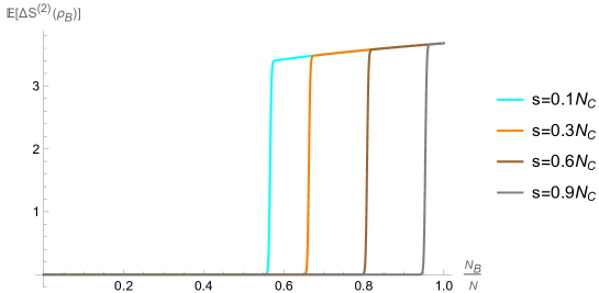
(a)

Figure 3: The averaged Rényi-2 entanglement asymmetry as a function of $\frac{N_{B}}{N}$ (c.f. eq. (5.5) or eq. (5.2)), where we take $N=500,N_{A}=15$. The maximum allowable value for $s$ is $N_{C}=N-N_{A}$.

6 Discussion and conclusion

Similar to the random pure state case [33], the behavior of entanglement asymmetry can be understood using the decoupling inequality. In our case, it reads

$$\left(\mathbb{E}_{U}[\|\rho_{B}-\rho_{B}^{\max}\|_{1}]\right)^{2}\leq\frac{d_{B}}{d_{D}}\textrm{tr}\rho_{AC}^{2},$$ (6.1)

where $\rho_{B}^{\max}=\frac{1}{d_{B}}I_{B}$ is the maximally mixed state on $B$ and

$$\rho_{AC}=\textrm{tr}_{R}\rho_{ACR}=\frac{1}{d_{A}}I_{A}\otimes\rho.$$ (6.2)

Therefore we have

$$\textrm{tr}\rho_{AC}^{2}=\frac{1}{d_{A}^{2}}\textrm{tr}(I_{A})~{}\textrm{tr}(\rho^{2})=\frac{2^{-s}}{d_{A}}.$$ (6.3)

Then the decoupling inequality eq. (6.1) becomes

$$\left(\mathbb{E}_{U}[\|\rho_{B}-\rho_{B}^{\max}\|_{1}]\right)^{2}\leq\frac{1}{2^{N+N_{A}+s-2N_{B}}},$$ (6.4)

which says that if $N_{B}<(N+N_{A}+s)/2$, then $\rho_{B}$ becomes almost maximally mixed while the maximally mixed state has vanishing entanglement asymmetry. Therefore we can conclude that the entanglement asymmetry of $\rho_{B}$ is almost vanishing for $N_{B}<(N+N_{A}+s)/2$. Our result is also applicable in the late-time regime of local unitary dynamics or even Hamiltonian dynamics.

In summary, in this paper, using the entanglement asymmetry as a modern tool to quantify symmetry breaking, we found a $U(1)$ symmetry of the radiation emerges before a certain transition time in the Hayden-Preskill thought experiment. We confirm this emergent symmetry by calculating the entanglement asymmetry of the radiation. We found the transition time depends on the initial entropy $s$ and the size of the diary $N_{A}$. When the black hole is maximally entangled with the early radiation, this emergent symmetry survives during the whole procedure of radiation. Using the decoupling inequality, we can understand our findings to some extent.

References

- [1] S. W. Hawking, “Particle Creation by Black Holes,” Commun. Math. Phys., vol. 43, pp. 199–220, 1975. [Erratum: Commun.Math.Phys. 46, 206 (1976)].
- [2] S. W. Hawking, “Breakdown of Predictability in Gravitational Collapse,” Phys. Rev. D, vol. 14, pp. 2460–2473, 1976.
- [3] D. Harlow, “Jerusalem Lectures on Black Holes and Quantum Information,” Rev. Mod. Phys., vol. 88, p. 015002, 2016.
- [4] A. Almheiri, T. Hartman, J. Maldacena, E. Shaghoulian, and A. Tajdini, “The entropy of Hawking radiation,” Rev. Mod. Phys., vol. 93, no. 3, p. 035002, 2021.
- [5] D. N. Page, “Average entropy of a subsystem,” Phys. Rev. Lett., vol. 71, pp. 1291–1294, 1993.
- [6] D. N. Page, “Information in black hole radiation,” Phys. Rev. Lett., vol. 71, pp. 3743–3746, 1993.
- [7] P. Hayden and J. Preskill, “Black holes as mirrors: Quantum information in random subsystems,” JHEP, vol. 09, p. 120, 2007.
- [8] B. Yoshida and A. Kitaev, “Efficient decoding for the Hayden-Preskill protocol,” 10 2017.
- [9] B. Yoshida and N. Y. Yao, “Disentangling Scrambling and Decoherence via Quantum Teleportation,” Phys. Rev. X, vol. 9, no. 1, p. 011006, 2019.
- [10] N. Bao and Y. Kikuchi, “Hayden-Preskill decoding from noisy Hawking radiation,” JHEP, vol. 02, p. 017, 2021.
- [11] Y. Cheng, C. Liu, J. Guo, Y. Chen, P. Zhang, and H. Zhai, “Realizing the Hayden-Preskill protocol with coupled Dicke models,” Phys. Rev. Res., vol. 2, no. 4, p. 043024, 2020.
- [12] L. Piroli, C. Sünderhauf, and X.-L. Qi, “A Random Unitary Circuit Model for Black Hole Evaporation,” JHEP, vol. 04, p. 063, 2020.
- [13] T. Hayata, Y. Hidaka, and Y. Kikuchi, “Diagnosis of information scrambling from Hamiltonian evolution under decoherence,” Phys. Rev. D, vol. 104, no. 7, p. 074518, 2021.
- [14] F. Ares, S. Murciano, and P. Calabrese, “Entanglement asymmetry as a probe of symmetry breaking,” Nature Commun., vol. 14, no. 1, p. 2036, 2023.
- [15] F. Ares, S. Murciano, E. Vernier, and P. Calabrese, “Lack of symmetry restoration after a quantum quench: An entanglement asymmetry study,” SciPost Phys., vol. 15, no. 3, p. 089, 2023.
- [16] S. Murciano, F. Ares, I. Klich, and P. Calabrese, “Entanglement asymmetry and quantum Mpemba effect in the XY spin chain,” J. Stat. Mech., vol. 2401, p. 013103, 2024.
- [17] C. Rylands, K. Klobas, F. Ares, P. Calabrese, S. Murciano, and B. Bertini, “Microscopic Origin of the Quantum Mpemba Effect in Integrable Systems,” Phys. Rev. Lett., vol. 133, no. 1, p. 010401, 2024.
- [18] C. Rylands, E. Vernier, and P. Calabrese, “Dynamical symmetry restoration in the Heisenberg spin chain,” 9 2024.
- [19] S. Liu, H.-K. Zhang, S. Yin, S.-X. Zhang, and H. Yao, “Quantum Mpemba effects in many-body localization systems,” 8 2024.
- [20] F. Ares, V. Vitale, and S. Murciano, “The quantum Mpemba effect in free-fermionic mixed states,” 5 2024.
- [21] M. Chen and H.-H. Chen, “Rényi entanglement asymmetry in (1+1)-dimensional conformal field theories,” Phys. Rev. D, vol. 109, no. 6, p. 065009, 2024.
- [22] M. Fossati, C. Rylands, and P. Calabrese, “Entanglement asymmetry in CFT with boundary symmetry breaking,” 11 2024.
- [23] F. Benini, V. Godet, and A. H. Singh, “Entanglement asymmetry in conformal field theory and holography,” 7 2024.
- [24] Y. Kusuki, S. Murciano, H. Ooguri, and S. Pal, “Entanglement asymmetry and symmetry defects in boundary conformal field theory,” 11 2024.
- [25] B. Bertini, K. Klobas, M. Collura, P. Calabrese, and C. Rylands, “Dynamics of charge fluctuations from asymmetric initial states,” Phys. Rev. B, vol. 109, no. 18, p. 184312, 2024.
- [26] S. Liu, H.-K. Zhang, S. Yin, and S.-X. Zhang, “Symmetry Restoration and Quantum Mpemba Effect in Symmetric Random Circuits,” Phys. Rev. Lett., vol. 133, no. 14, p. 140405, 2024.
- [27] X. Turkeshi, P. Calabrese, and A. De Luca, “Quantum Mpemba Effect in Random Circuits,” 5 2024.
- [28] A. Foligno, P. Calabrese, and B. Bertini, “Non-equilibrium dynamics of charged dual-unitary circuits,” 7 2024.
- [29] L. K. Joshi et al., “Observing the Quantum Mpemba Effect in Quantum Simulations,” Phys. Rev. Lett., vol. 133, no. 1, p. 010402, 2024.
- [30] E. Bianchi and P. Dona, “Typical entanglement entropy in the presence of a center: Page curve and its variance,” Phys. Rev. D, vol. 100, no. 10, p. 105010, 2019.
- [31] S. Murciano, P. Calabrese, and L. Piroli, “Symmetry-resolved Page curves,” Phys. Rev. D, vol. 106, no. 4, p. 046015, 2022.
- [32] P. H. C. Lau, T. Noumi, Y. Takii, and K. Tamaoka, “Page curve and symmetries,” JHEP, vol. 10, p. 015, 2022.
- [33] F. Ares, S. Murciano, L. Piroli, and P. Calabrese, “Entanglement asymmetry study of black hole radiation,” Phys. Rev. D, vol. 110, no. 6, p. L061901, 2024.
- [34] A. Russotto, F. Ares, and P. Calabrese, “Non-Abelian entanglement asymmetry in random states,” 11 2024.
- [35] R. Li and J. Wang, “Hayden-Preskill protocol and decoding Hawking radiation at finite temperature,” Phys. Rev. D, vol. 106, no. 4, p. 046011, 2022.