Ensemble reliability and the signal-to-noise paradox in large-ensemble subseasonal forecasts

Abstract

Recent studies have suggested the existence of a ‘signal-to-noise paradox’ (SNP) in ensemble forecasts that manifests as situations where the correlation between the forecast ensemble mean and the observed truth is larger than the correlation between the forecast ensemble mean and individual forecast members. A perfectly reliable ensemble, in which forecast members and observations are drawn from the same underlying probability distribution, will not exhibit an SNP if sample statistics can be evaluated using a sufficiently large ensemble size ($N$) over a sufficiently large number of independent cases ($M$). However, when $M$ is finite, an apparent SNP will sometimes occur as a natural consequence of sampling uncertainty, even in a perfectly reliable ensemble with many members. In this study, we evaluate the forecast skill, reliability characteristics, and signal-to-noise properties of three large-scale atmospheric circulation indices in 100-member subseasonal reforecasts. Consistent with recent studies, this reforecast dataset exhibits an apparent SNP in the North Atlantic Oscillation (NAO) at subseasonal lead times. However, based on several lines of evidence, we conclude that the apparent paradox in this dataset is a consequence of large observational sampling uncertainties that are insensitive to ensemble size and common to all model comparisons over the same period. Furthermore, we demonstrate that this apparent SNP can be eliminated by application of an unbiased reliability calibration. However, this is achieved through overfitting such that sample statistics from calibrated forecasts inherit the large sampling uncertainties present in the observations and thus exhibit unphysical variations with lead time. Finally, we make several recommendations for the robust and unbiased evaluation of reliability and signal-to-noise properties in the presence of large sampling uncertainties.

Keywords Subseasonal, seasonal, S2S, predictability, ensemble, reliability, signal, noise, paradox

1 Introduction

Ensemble forecast systems are widely used to generate probabilistic weather and climate predictions at lead times of days to decades (e.g. Molteni et al., 1996; Palmer et al., 2005; Doblas-Reyes et al., 2009; Vitart and Robertson, 2018; Smith et al., 2019). The origins, motivations, and practicalities of ensemble forecasting are comprehensively described by Lewis (2005) and Leutbecher and Palmer (2008). An important metric for the quality of probabilistic forecasts is their reliability, which requires that the observed frequency of an event tends to $p$ when averaged over many cases for which the event was predicted to occur with probability $p$ (Johnson and Bowler, 2009; Leutbecher and Palmer, 2008; Weisheimer and Palmer, 2014). Forecast reliability is commonly assessed in short- and medium-range ensemble forecasts using a combination of probabilistic verification metrics and comparison of the average ensemble variance with the average squared error of the ensemble mean (e.g. Whitaker and Loughe, 1998; Scherrer et al., 2004; Hopson, 2014; Yamaguchi et al., 2016; Rodwell et al., 2018).

In contrast, the seasonal-to-decadal forecasting community often emphasises correlation-based evaluation of ensemble mean forecasts, with particular attention given to situations that exhibit the so-called ‘signal-to-noise paradox’ (SNP; Eade et al., 2014; Scaife and Smith, 2018). The SNP manifests as a counterintuitive situation where the correlation between the forecast ensemble mean and the observed truth is larger than the correlation between the forecast ensemble mean and individual forecast members, and thus the real world appears to be more predictable than individual ensemble members from the same forecast model. An apparent SNP has been identified in a variety of ensemble forecasting systems covering subseasonal to multi-decadal timescales (Eade et al., 2014; Scaife and Smith, 2018; Smith et al., 2019; Garfinkel et al., 2024) and is particularly evident for predictions of the wintertime North Atlantic Oscillation (NAO; Baker et al., 2018). Of particular relevance to the present work is a recent study by Garfinkel et al. (2024), which diagnoses an apparent SNP in subseasonal reforecasts produced by several models. However, this study relies on reforecasts with relatively small ensemble sizes and the relevant sample statistics do not include uncertainty estimates. As we will demonstrate, robust estimates of sampling uncertainty are crucial when considering whether a forecasting system exhibits a statistically robust SNP.

There is no scientific consensus on the origins or interpretation of the SNP (Weisheimer et al., 2024). Several studies have proposed physical interpretations of the SNP, including deficiencies in the representation of tropical-extratropical teleconnections (Scaife and Smith, 2018; Garfinkel et al., 2022), underestimated persistence of non-linear regimes (Strommen and Palmer, 2019; Zhang and Kirtman, 2019), weak transient eddy feedbacks (Scaife et al., 2019; Hardiman et al., 2022), and inadequate representation of air-sea coupling (Zhang et al., 2021). Other studies have emphasised statistical interpretations, including the links to reliability and the sensitivity of correlation-based metrics to sampling uncertainty (Shi et al., 2015; Weisheimer et al., 2019; Bröcker et al., 2023; Strommen et al., 2023).

In this study, we evaluate forecast skill, reliability characteristics, and signal-to-noise properties for three large-scale atmospheric circulation indices in 100-member subseasonal reforecasts with the European Centre for Medium-Range Weather Forecasts (ECMWF) Integrated Forecasting System (IFS). There are several novelties to our approach, including (i) the use of large-ensemble subseasonal forecasts, (ii) the careful application of unbiased statistical methods (e.g. Roberts and Leutbecher, 2024), (iii) our emphasis on physically plausible changes with forecast lead time, and (iv) the use of reliability calibration to distinguish between predictable signals that are too weak and unpredictable noise that is too strong. We use this large-ensemble reforecast dataset to answer the following questions:

1. Are ECMWF subseasonal forecasts reliable?

2. Do ECMWF subseasonal forecasts exhibit the symptoms of an SNP? If yes, in which indices and at what lead times does this apparent paradox emerge?

3. Does reliability calibration provide any insights into the origins of the SNP?

4. Are the answers to the above questions robust to the impacts of sampling uncertainty?

The remainder of this paper is organised as follows: Section 2 describes the ECMWF subseasonal reforecast dataset and the calculation of large-scale atmospheric circulation indices. Section 3 provides an overview of the statistical concepts that are relevant for this study. Section 4 evaluates the forecast skill, reliability characteristics, and signal-to-noise properties in uncalibrated forecasts. Section 5 evaluates the same, but in forecasts that have been calibrated to enforce reliability. Lastly, section 6 summarises our results and provides recommendations for the robust and unbiased evaluation of reliability and signal-to-noise properties in the presence of sampling uncertainties.

2 Data

2.1 IFS reforecasts

We evaluate forecast skill, ensemble reliability, and signal-to-noise properties at subseasonal timescales using 100-member reforecasts performed with cycle 47r3 of the ECMWF IFS, which includes dynamic representations of the atmosphere, ocean, sea-ice, land-surface, and ocean waves. IFS cycle 47r3 was used operationally at ECMWF from October 12th 2021 to June 27th 2023, when it was replaced by IFS cycle 48r1. Roberts et al. (2023) provide a more thorough description of IFS cycle 47r3, including an overview of the operational subseasonal reforecast configuration. Here, we use an experimental reforecast configuration comprised of 46-day, 100-member ensemble forecasts initialised every February 1st, May 1st, August 1st, and November 1st between 2001 and 2020 for a total of 80 start dates. We exclude the unperturbed control forecast (i.e. member 0) from our analysis as it is not statistically exchangeable with perturbed members. The atmospheric model uses the cubic octahedral reduced Gaussian grid with 137 vertical levels and a horizontal resolution of Tco319 (i.e., an average grid spacing of $\sim$35 km ) at all lead times. Otherwise, the IFS configuration, initialization strategy, stochastic parameterizations, and ocean/sea-ice coupling are exactly as described for the operational reforecast configuration used by Roberts et al. (2023) and will not be repeated here. Reforecasts are verified using data from the ERA5 reanalysis (Hersbach et al., 2020).

2.2 Atmospheric circulation indices

We focus our analysis of reliability and signal-to-noise properties on three indices that measure different aspects of the large-scale tropospheric and stratospheric circulation in the Northern Hemisphere. In addition, we evaluate tropical-extratropical teleconnections using lagged composites conditioned on different phases of the Madden-Julian Oscillation (MJO). A brief definition of each index is provided below.

2.2.1 The North Atlantic Oscillation (NAO)

The North Atlantic Oscillation (NAO) is a large-scale mode of atmospheric variability associated with widespread variations in surface weather conditions across Europe and the North Atlantic (Hurrell, 1995). For each forecast start date, we calculate NAO indices for each forecast member and the equivalent dates in ERA5 by projecting 500 hPa geopotential height anomalies on a regular 2.5^∘ $\times$ 2.5^∘ latitude-longitude grid onto a precomputed loading pattern. The NAO loading pattern is defined as the first empirical orthogonal function (EOF) of all-year monthly mean 500 hPa geopotential height anomalies for the period 1979-2018 in the ERA-interim reanalysis (Dee et al., 2011) for the region bounded by 20^∘N-80^∘N and 90^∘W-40^∘E. EOFs are calculated using the Python ‘eofs’ package (Dawson, 2016) and anomalies are weighted by $\sqrt{\textnormal{cos}(\textnormal{latitude})}$ prior to computation to account for variations in grid-cell area. Forecasts and reanalysis anomalies are projected onto the same observation-based loading pattern and the resulting indices are divided by a precomputed scaling factor, which is defined such that indices can be interpreted as the standardised principal component time-series associated with the EOF-based NAO pattern. The main conclusions of our study are not sensitive to this specific definition of the NAO, and also apply to EOF-based NAO indices derived from mean sea level pressure.

2.2.2 The Pacific-North American pattern (PNA)

The Pacific-North American pattern (PNA) is another large-scale mode of Northern Hemisphere atmospheric variability associated with coherent variations in temperature and precipitation over the North American continent (Leathers et al., 1991). We calculate PNA indices following the same procedure outlined above for the NAO. The only difference is that loading patterns are defined from first EOF of monthly mean 500 hPa geopotential height anomalies for the region bounded by 10^∘N-80^∘N and 150^∘E-300^∘E.

2.2.3 The Northern Hemisphere Stratospheric Polar Vortex (PVORTEX)

Previous studies have demonstrated that anomalies in the strength of the Northern Hemisphere stratospheric polar vortex can propagate downwards and influence evolution of tropospheric weather regimes such as the NAO (Baldwin and Dunkerton, 1999; Polvani and Waugh, 2004; Ineson and Scaife, 2009). We quantify the strength of the Northern Hemisphere stratospheric polar vortex (PVORTEX) in IFS reforecasts and ERA5 as described in Roberts et al. (2023), which is consistent with indices used in previous studies to investigate causal links between the troposphere and Northern Hemisphere sudden stratospheric warmings (e.g. Limpasuvan et al., 2004; Barnes et al., 2019). Specifically, indices are calculated from the zonal mean of zonal wind anomalies at 50 hPa and 60^∘N and standardised by dividing with a constant factor of 5.15 ms^-1, which corresponds to the standard deviation of the raw vortex index calculated using all-year daily values from the ERA-interim reanalysis (Dee et al., 2011) for the period 1979-2018.

2.2.4 The Madden–Julian oscillation (MJO)

The Madden-Julian Oscillation (MJO) is the leading mode of intraseasonal variability in the tropics (Madden and Julian, 1971) and an important source of predictability at subseasonal lead times. Variations in tropical convective heating and upper atmosphere circulation anomalies associated with the MJO provide a source of Rossby waves that drive global teleconnections (Hoskins and Karoly, 1981; Sardeshmukh and Hoskins, 1988; Cassou, 2008; Lin et al., 2009). We diagnose MJO variability using the real-time multivariate MJO (RMM) index following Wheeler and Hendon (2004) and Gottschalck et al. (2010). The two components of the bivariate index (RMM1 and RMM2) are derived by projecting daily mean anomalies onto the two leading observation-based multivariate EOFs of meridionally averaged (15^∘S-15^∘N) zonal winds at 850 hPa and 200 hPa and outgoing long wave radiation (OLR). MJO amplitude and phase are defined as $\sqrt{\textnormal{RMM1}^{2}+\textnormal{RMM2}^{2}}$ and $\textnormal{arctan}(\textnormal{RMM1},\textnormal{RMM2})$, respectively. Phase numbers correspond to the different sectors of MJO phase diagram and are indicative of MJO activity over the Indian Ocean (phases 2 and 3), maritime continent (phases 4 and 5), western Pacific Ocean (phases 6 and 7), and the Atlantic Ocean/Africa (phases 8 and 1).

3 Statistical concepts

Throughout this study, we emphasise the use of unbiased approaches to ensure that our conclusions are unaffected by erroneous assumptions regarding the exchangeability (or otherwise) of observations and forecasts. To introduce the statistical concepts central to this study, we consider an idealised perfectly reliable ensemble forecast system with $k=1,\dots,N$ members covering $j=1,\dots,M$ independent cases (e.g. forecast start dates). In this idealised system, ensemble forecast members ($x_{1,j},\dots,x_{N,j}$) and the observed truth ($x_{T,j}$) are drawn from the same underlying probability distribution at each start date such that they are statistically exchangeable.

3.1 Anomaly calculation

We define ensemble forecast anomalies ($z_{k,j}$) and observed anomalies ($z_{T,j}$) following ‘method D’ of Roberts and Leutbecher (2024) such that

$$z_{k,j}=x_{k,j}-\frac{1}{L-1}\sum\limits^{L}_{\begin{subarray}{c}h=1\\ h\neq j\end{subarray}}x_{k,h},$$ (1)

$$z_{T,j}=x_{T,j}-\frac{1}{L-1}\sum\limits^{L}_{\begin{subarray}{c}h=1\\ h\neq j\end{subarray}}x_{T,h},$$ (2)

where $L$ is the number of years in the reforecast data set and $h=1,\dots,L$ represents the subset of all cases with the same calendar start date as case $j$. Anomalies are thus calculated relative to climatologies estimated separately for each member and each start date. Crucially, calculating forecast anomalies separately for each member ensures that forecast and verification anomalies are defined relative to reference climatologies with the same sampling uncertainty. This approach has no impact on ensemble means, but ensures that forecast member anomalies remain statistically exchangeable with observed anomalies if the underlying raw forecasts are perfectly reliable. This is not the case for standard approaches to anomaly calculation, which calculate forecast anomalies with respect to a climatology that includes all members. Importantly, this effect is also present for statistics that are not defined in terms of ensemble forecast anomalies but still require the removal of an estimate of the sample mean (e.g. variances, correlations). The statistical justification and motivations for this approach to ensemble forecast anomaly calculation are described in detail by Roberts and Leutbecher (2024). Unless otherwise specified, all statistical quantities in this paper are derived from anomalies calculated following the definitions for $z_{k,j}$ and $z_{T,j}$.

3.2 Ensemble reliability

Johnson and Bowler (2009) emphasise that perfectly reliable anomaly-based ensemble forecasts have certain statistical properties, which can be derived from the requirement that observations and forecast members are interchangeable. The first property is that the total variance of the observed truth ($\sigma_{T}^{2}=\mathbb{E}\left[z_{T,j}^{2}\right]$) should be equal to the total variance of the ensemble forecast members ($\sigma_{z}^{2}=\mathbb{E}\left[\left<z_{.,j}^{2}\right>_{N}\right]$) when evaluated over many cases such that

$$\lim_{M\to\infty}\frac{1}{M}\sum^{M}_{j=1}z_{T,j}^{2}=\frac{1}{M}\sum^{M}_{j=1}\left<z_{.,j}^{2}\right>_{N},$$ (3)

where $\mathbb{E}\left[\cdot\right]$ is the expecation over cases $j$, $\mathbb{E}\left[z_{T,j}\right]=\mathbb{E}\left[z_{k,j}\right]=0$, and $\left<\cdot\right>_{N}$ represents the mean over a sample of $N$ members such that the ensemble mean for case $j$ is denoted $\left<z_{.,j}\right>_{N}\equiv\frac{1}{N}\sum^{N}_{k=1}z_{k,j}$. Following Van Schaeybroeck and Vannitsem (2015) and Roberts and Leutbecher (2024), we refer to this statistical property as climatological reliability.

The second property is that, with appropriate unbiased estimators, the square root of the mean ensemble variance (i.e. ‘spread’) will converge with the root-mean-square error (RMSE) of the ensemble mean such that

$$\lim_{M\to\infty}\left(\frac{\textnormal{Spread}}{\textnormal{RMSE}}\right)_{\textnormal{unbiased}}=\sqrt{\left(\frac{N+1}{N-1}\right)}\frac{\sqrt{\frac{1}{M}\sum^{M}_{j=1}\left<\left(z_{.,j}-\left<z_{.,j}\right>_{N}\right)^{2}\right>_{N}}}{\sqrt{\frac{1}{M}\sum^{M}_{j=1}\left(z_{T,j}-\left<z_{.,j}\right>_{N}\right)^{2}}}=1,$$ (4)

where the factor of $\sqrt{\frac{N+1}{N-1}}$ ensures estimates are unbiased with ensemble size as discussed by Leutbecher and Palmer (2008). We refer to this spread-error relationship as ensemble variance reliability.

3.3 Correlations

Johnson and Bowler (2009) also highlighted the links between reliability and correlation-based evaluation of ensemble mean forecasts by considering the impact of a simple member-by-member statistical calibration that enforces ensemble reliability. They showed that, in the limit $M\rightarrow\infty$ and $N\rightarrow\infty$, a calibration that simultaneously enforces climatological reliability (equation 3) and ensemble variance reliability (equation 4) is exactly equivalent to a calibration that enforces equation 3 combined with the constraint that the correlation between the forecast ensemble mean and observations ($r_{fo}$) is equal to the correlation between forecast ensemble mean and forecast members ($r_{ff}$). For a finite ensemble size, the relevant correlations can be defined as follows

$$r_{fo}=\frac{\mathbb{E}\left[\left<z_{.,j}\right>_{N-1}z_{T,j}\right]}{\sqrt{\mathbb{E}\left[\left<z_{.,j}\right>_{N-1}^{2}\right]\mathbb{E}\left[z_{T,j}^{2}\right]}},$$ (5)

$$r_{ff(k)}=\frac{\mathbb{E}\left[\left<z_{.,j}\right>_{N-1}^{i\neq k}z_{k,j}\right]}{\sqrt{\mathbb{E}\left[\left(\left<z_{.,j}\right>_{N-1}^{i\neq k}\right)^{2}\right]\mathbb{E}\left[z_{k,j}^{2}\right]}},$$ (6)

$$r_{ff}=\frac{1}{N}\sum\limits^{N}_{k=1}r_{ff(k)},$$ (7)

where we define $\left<\cdot\right>_{N-1}$ to indicate the ensemble mean constructed from the first $N-1$ members and $\left<\cdot\right>_{N-1}^{i\neq k}\equiv\frac{1}{N-1}\sum\limits^{N}_{\begin{subarray}{c}i=1\\ i\neq k\end{subarray}}$ such that $\left<z_{.,j}\right>_{N-1}^{i\neq k}$ represents the ensemble mean for case $j$ after excluding member $k$. The value of $r_{ff(k)}$ thus represents the correlation between the forecast ensemble mean and an excluded ensemble member and $r_{ff}$ represents the mean of $N$ estimates of $r_{ff(k)}$. We use this definition of $r_{ff(k)}$ for consistency with $r_{fo}$, for which the forecast ensemble means do not include the observed value. Importantly, we also calculate $r_{fo}$ using an ensemble mean constructed from $N-1$ members for consistency with $r_{ff(k)}$. The use of $N-1$ rather than $N$ members ensures that estimate of $r_{fo}$ are exchangeable with estimates of $r_{ff(k)}$ in a perfectly reliable ensemble. For small ensemble sizes, calculating $r_{fo}$ with $N$ members and $r_{ff(k)}$ with $N-1$ members could lead to misdiagnosis of an SNP.

We also note that equations 6 and 7 are not the only way to estimate $r_{ff}$. In a well-constructed ensemble, the members for case $j$ can be considered independent draws from the same underlying probability distribution and there is no particular reason that $r_{ff(k)}$ should be estimated using the same member $k$ from each case $j$. For example, $r_{ff(k)}$ could also be estimated by randomly selecting a member to exclude from the ensemble mean for each case $j$. Nevertheless, selecting the same member $k$ for each case $j$ is straightforward to calculate and provides an unbiased estimate of the quantity of interest.

3.4 The ratio of predictable components

As described in section 1, the relationship between $r_{fo}$ and $r_{ff}$ in ensemble forecasting systems has drawn significant attention in the climate forecasting community in the context of the SNP (Eade et al., 2014; Scaife and Smith, 2018). The SNP was originally diagnosed using the ratio of predictable components (RPC; Eade et al., 2014) defined in terms of $r_{fo}$, $\sigma_{z}^{2}$, and $\sigma_{\left<z\right>}^{2}=\mathbb{E}\left[\left<z_{.,j}\right>_{N}^{2}\right]$ as

$$\textnormal{RPC}\geq\frac{r_{fo}}{\sqrt{\sigma_{\left<z\right>}^{2}/\sigma_{z}^{2}}}.$$ (8)

An alternative expression for RPC can be defined directly from correlations (Scaife and Smith, 2018) as

$$\textnormal{RPC}_{\textnormal{Corr}}=\sqrt{\frac{r_{fo}^{2}}{r_{ff}^{2}}}.$$ (9)

In both forms, an RPC value exceeding one has been interpreted as a predictability paradox. However, as discussed below, direct comparison of $r_{fo}$ and $r_{ff}$ can lead to misdiagnosis of the SNP when considering sample statistics estimated from a finite number of independent cases.

3.5 Ensemble calibration

To explore the links between ensemble reliability and the SNP, we use an unbiased member-by-member calibration approach that simultaneously enforces climatological reliability (equation 3) and ensemble variance reliability (equation 4). This calibration ensures that forecast anomalies satisfy equations 3 and 4, which are properties of a perfectly reliable ensemble, when averaged over a sample of start dates. However, the resulting calibrated forecasts will not (in general) be perfectly reliable such that ensemble forecast members and the observed truth can be considered drawn from the same underlying probability distribution for each start date. Calibrated forecast anomalies ($\hat{z}_{k,j}$) are derived by separately modifying the ensemble mean and perturbations from the ensemble mean as follows

$$\hat{z}_{k,j}=\alpha\left<z_{.,j}\right>_{N}+\beta\left(z_{k,j}-\left<z_{.,j}\right>_{N}\right),$$ (10)

where

$$\alpha=\frac{\sigma_{T}}{\sigma_{\left<z\right>}}\left(\frac{r_{fo}+\sqrt{r_{fo}^{2}+R^{2}-1}}{R+1}\right)$$ (11)

$$\beta^{2}=\frac{\sigma_{T}^{2}-\alpha^{2}\sigma_{\left<z\right>}^{2}}{\mathbb{E}[(z_{k,j}-\left<z_{.,j}\right>_{N})^{2}]}$$ (12)

and $R=\frac{N+1}{N-1}$. This formulation follows Johnson and Bowler (2009) but the parameters $\alpha$ and $\beta$ are estimated following Roberts and Leutbecher (2024) such that they are unbiased with ensemble size resulting in ensemble forecasts that exactly satisfy the climatological reliability and unbiased ensemble variance reliability conditions described in section 3.2, even for small ensemble sizes.

The parameters $\alpha$ and $\beta$ can be directly related to previous work, which has demonstrated that a ‘perfect’ RPC can be recovered using post-processing methods that separately scale the predictable (i.e. ensemble mean) and unpredictable (i.e. deviations from the ensemble mean) components of an ensemble forecast (e.g. Eade et al., 2014). In this framework, an apparent SNP can occur either because the predictable signal is too weak (i.e. the diagnosed value of $\alpha>1$) or the unpredictable noise is too large (i.e. the diagnosed value of $\beta<1$).

3.6 Sampling uncertainty

Throughout this study we emphasise the importance of robust estimates of sampling uncertainty. A perfectly reliable ensemble, in which forecast members and observations are statistically exchangeable, will not exhibit an SNP if sample statistics can be evaluated using a sufficiently large ensemble over a sufficiently large number of independent cases. However, in real-world forecasting scenarios, an apparent SNP will sometimes occur as a natural consequence of sampling uncertainty. In a perfectly reliable ensemble, sample estimates of $r_{ff}$, $r_{ff(k)}$, and $r_{fo}$ will converge with the underlying population correlation, $\rho$, with increasing $M$, and $N$. We thus expect RPC${}_{\textnormal{Corr}}$ $\rightarrow$ 1 as M $\rightarrow\infty$ and N $\rightarrow\infty$. However, the impact of sampling uncertainties associated with finite $M$ mean that RPC${}_{\textnormal{Corr}}$ $>1$ will sometimes occur even in a perfectly reliable ensemble with many members.

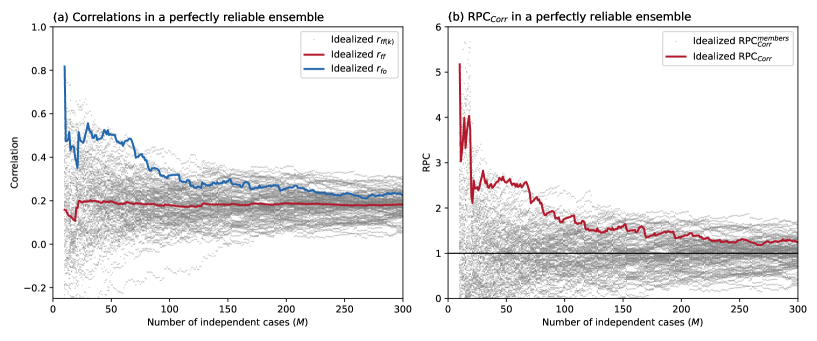
Figure 1: (a) Correlations calculated from an idealised perfectly reliable ensemble data set. Forecast and observations are generated by the same process such that $z_{k,j}=s_{j}+n_{k,j}$, where $s_{j}\sim\mathcal{N}(0,\,1^{2})$ is a predictable component common to all members and observations and $n_{k,j}\sim\mathcal{N}(0,\,4.9^{2})$ is an unpredictable noise component, such that $\rho=0.2$. The presented values are calculated for $M=10,...,300$ cases using $N=100$ members. These values and the random seed have been chosen to give $r_{ff}\approx 0.2$ and $r_{fo}\approx 0.4$ for $M=80$ and $N=100$, which are equivalent to the values estimated for the NAO at a lead time of $\sim$35 days in figure 3. (b) Idealised estimates of RPC_Corr calculated from the values of $r_{ff}$ and $r_{fo}$ in panel (a). RPC${}_{Corr}^{member}$ is calculated by separately treating each member as the observed truth. In this perfectly reliable ensemble scenario, the values of RPC${}_{Corr}^{member}$ can be considered additional samples from the same underlying distribution that generated RPC_Corr.

To illustrate this concept, figure 1 shows correlations and RPC_Corr calculated using an idealised 100-member perfectly reliable ensemble data set generated for a process with intrinsic predictability $\rho=0.2$. When the number of forecast start dates is limited (i.e. $M<50$), it is possible to identify scenarios where $r_{fo}>0.5$ and thus RPC${}_{Corr}>2.5$, despite $r_{fo}$ lying within the distribution of estimates of $r_{ff(k)}$. Importantly, uncertainty in $r_{fo}$ is typically much larger than $r_{ff}$, which represents an average of $N$ estimates of $r_{ff(k)}$.

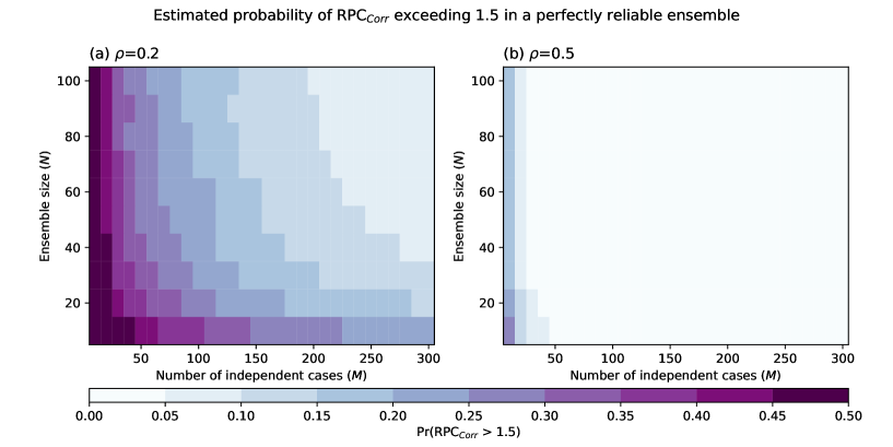
Figure 2: Estimated probability that RPC_Corr exceeds a threshold value of 1.5 in idealised perfectly reliable ensembles as function of the number of independent cases ($M$), ensemble size ($N$), and different levels of intrinsic correlation skill ($\rho$). Each estimate of Pr(RPC${}_{Corr}>1.5$) is derived from a distribution of 10,000 RPC_Corr values generated using the idealised statistical model that produces exchangeable forecast members and observations as described in the caption of figure 1.

To further illustrate this point, figure 2 shows the probability of RPC_Corr exceeding a threshold value of 1.5 as a function of $M$ and $N$ in an idealised perfectly reliable ensemble. When intrinsic predictability is low (i.e. $\rho=0.2$), there is a 30-35% chance of RPC_Corr exceeding 1.5 for $N=100$ and $M=30$, even when forecasts and observations are generated by the same statistical process. This is reduced to $\sim$5% if RPC_Corr is evaluated using $N=100$ and $M=300$. If intrinsic predictability is modest (i.e. $\rho=0.5$), the probability of detecting RPC${}_{Corr}>1.5$ is dramatically reduced (figure 2b). If intrinsic predictability is high (i.e. $\rho>0.7$) and $M$ and $N$ are sufficiently large such that $r_{ff}\to\rho$, then RPC${}_{Corr}>1.5$ becomes impossible. These results are consistent with the analysis of Bröcker et al. (2023), which demonstrated that RPC and RPC${}_{\textnormal{Corr}}$ are particularly sensitive to sampling uncertainty in $\sigma_{T}$ when $r_{ff}$ is small. We emphasise that a perfectly reliable ensemble forecast with a large ensemble size can still exhibit RPC${}_{Corr}>1$ if not evaluated using a sufficiently large number of independent cases. For this reason, robust diagnosis of an SNP should include demonstration that $r_{fo}$ does not plausibly lie within the distribution of estimates of $r_{ff(k)}$.

4 Results for uncalibrated forecasts

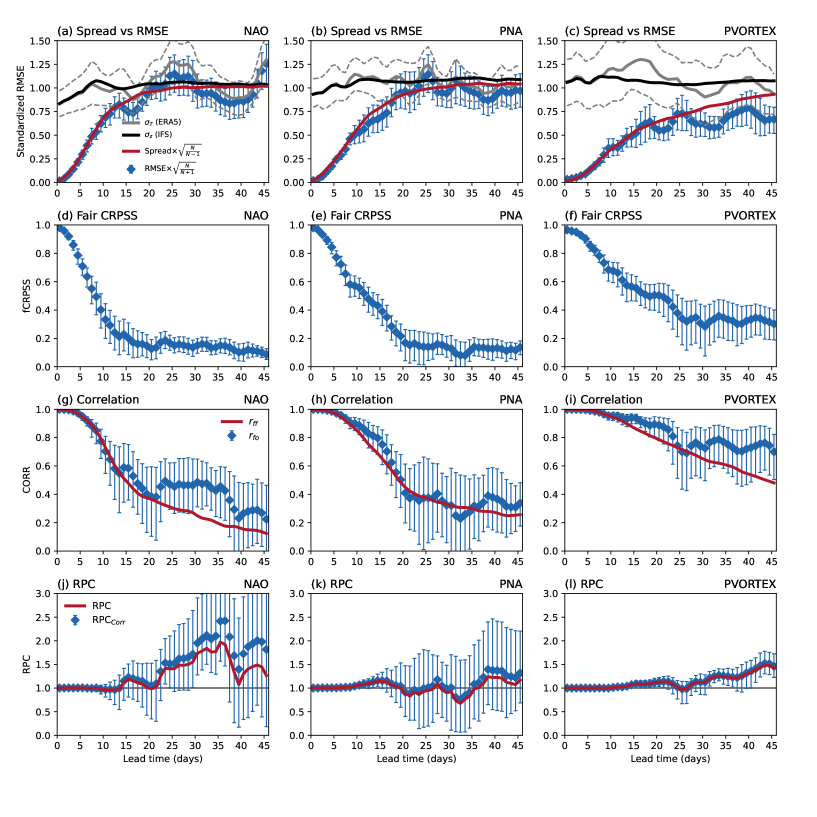
Figure 3: Forecast and verification statistics for three atmosphere circulation indices derived from uncalibrated daily mean anomalies. (a-c) Total anomaly variability in IFS reforecasts ($\sigma_{z}$) and the ERA5 reanalysis ($\sigma_{T}$), root-mean-square error of ensemble mean anomaly forecasts (RMSE), and the square root of mean ensemble variance (SPREAD). RMSE and SPREAD are scaled by $\sqrt{\frac{N}{N+1}}$ and $\sqrt{\frac{N}{N-1}}$, respectively, to provide estimates that are unbiased with ensemble size (Leutbecher and Palmer, 2008). (d-f) Fair version of the continuous ranked probability skill score (fCRPSS) calculated as $\textnormal{fCRPSS}=1-\frac{\textnormal{fCRPS}}{\textnormal{CRPS}_{\textnormal{clim}}}$, where fCRPS is the fair version of the continuous ranked probability score (Ferro, 2014) and CRPS${}_{\textnormal{clim}}$ is a reference score derived from the climatological distribution of observed anomalies. (g-i) Correlation between the forecast ensemble mean and observations ($r_{fo}$) and the mean correlation between forecast ensemble mean and an excluded forecast member ($r_{ff}$) calculated as described in section 3. (j-l) The ratio of predictable components calculated using both methods described in section 3. Sampling uncertainties are estimated using a bootstrap resampling approach whereby scores are calculated 500 times using randomly selected (with replacement) start dates. Error bars or dashed lines represent the 2.5th and 97.5th percentiles of the resulting distributions.

The reliability characteristics of daily mean NAO, PNA, and PVORTEX forecasts are summarised in figure 3. In general, there is good agreement between ERA5 and IFS estimates of total NAO variability such that estimates of $\sigma_{z}$ lie within the 95% confidence intervals of $\sigma_{T}$ across all lead times (figure 3a). Similarly, the ensemble spread of NAO forecasts lies within the 95% confidence intervals of RMSE for almost all lead times. PNA forecasts also show good agreement between IFS and ERA5 estimates of total variability and a close correspondence between spread and RMSE (figure 3b). Based on these comparisons, we conclude that daily mean NAO and PNA forecasts satisfy the climatological and ensemble variance criteria described in section 3.2 within the tolerance of our estimated sampling uncertainties. In contrast, although PVORTEX forecasts show good agreement between $\sigma_{T}$ and $\sigma_{z}$ across all lead times, they become significantly over-dispersive (i.e. spread > RMSE) at lead times greater than 25 days (figure 3c).

For NAO and PNA forecasts, ensemble spread increases smoothly and monotonically with lead time before saturating and converging with estimates of $\sigma_{z}$. PVORTEX forecasts also show a smooth and monotonic increase in spread with lead time, but it does not saturate within the duration of the 46-day forecasts due to the higher predictability of this stratospheric index. The mean correlation between the forecast ensemble mean and an excluded ensemble member ($r_{ff}$) also reduces smoothly with lead time in all three indices due to the gradual loss of predictability at longer time scales (figure 3g-i). In contrast, RMSE, $\sigma_{T}$, and correlations between forecast ensemble means and observations ($r_{fo}$) exhibit unphysical variations with lead time, which is a consequence of the much larger sampling uncertainty in the verifying observations compared to the 100-member forecast ensemble. The variability in forecast skill with lead time is less evident in the probabilistic continuous ranked probability skill score (CRPSS; figure 3d-f), which measures the skill of the entire forecast distribution relative to a climatological reference forecast.

The evolution of spread, RMSE, CRPSS, and $r_{ff}$ with lead time provide a consistent characterization of the relative predictability of the three circulation indices in IFS reforecasts. For example, it takes $\sim$10 days for NAO forecasts to reach a threshold CRPSS value of 0.4. In contrast, PNA and PVORTEX indices are more predictable and reach this threshold value after $\sim$15 and $\sim$25 days, respectively. The order of diagnosed predictability (PVORTEX $>$ PNA $>$ NAO) does not change if timescales are instead diagnosed from threshold values of RMSE, ensemble spread, or $r_{ff}$. The exact thresholds and absolute timescales used for this comparison are not critical for diagnosing the relative predictability of each index.

Estimates of predictability derived from $r_{fo}$ are a notable outlier as the NAO is seemingly more predictable than the PNA at some lead times. For PNA forecasts, $r_{ff}$ and $r_{fo}$ are generally consistent and thus RPC $\approx 1$ and RPC${}_{\textnormal{Corr}}\approx 1$ for all forecast lead times (figure 3k). In contrast, there are significant differences between $r_{ff}$ and $r_{fo}$ in NAO and PVORTEX forecasts at lead times greater than 20 days (figures 3j and 3l). In particular, NAO forecasts exhibit an unphysical increase in $r_{fo}$ from $\sim$0.40 at day 20 to $\sim$0.46 at day 30 whereas $r_{ff}$ decreases from $\sim$0.38 to $\sim$0.27 over the same lead times. These differences between $r_{ff}$ and $r_{fo}$ in NAO forecasts result in RPC and RPC${}_{\textnormal{Corr}}$ values reaching $\sim$2.5 and thus an apparent SNP at some lead times (e.g. days 31 to 37). Similarly, $r_{fo}$ is significantly higher than $r_{ff}$ for some lead times in PVORTEX forecasts (e.g. days 43-46) such that RPC and RPC${}_{\textnormal{Corr}}$ reach a maximum value of $\sim$1.5.

However, as was emphasised in section 3.6, RPC${}_{Corr}>1$ can occur in the absence of an SNP paradox as $r_{ff}$ and $r_{fo}$ have different sampling uncertainties such that they are not generally statistically interchangeable, even in a perfectly reliable ensemble. For this reason, robust diagnosis of an SNP should also include demonstration that $r_{fo}$ is not plausibly drawn from the distribution of model-model correlations between the forecast ensemble mean and an excluded ensemble member given by $r_{ff(k)}$. This aspect of the SNP cannot be evaluated using the definitions of RPC presented in section 3.4.

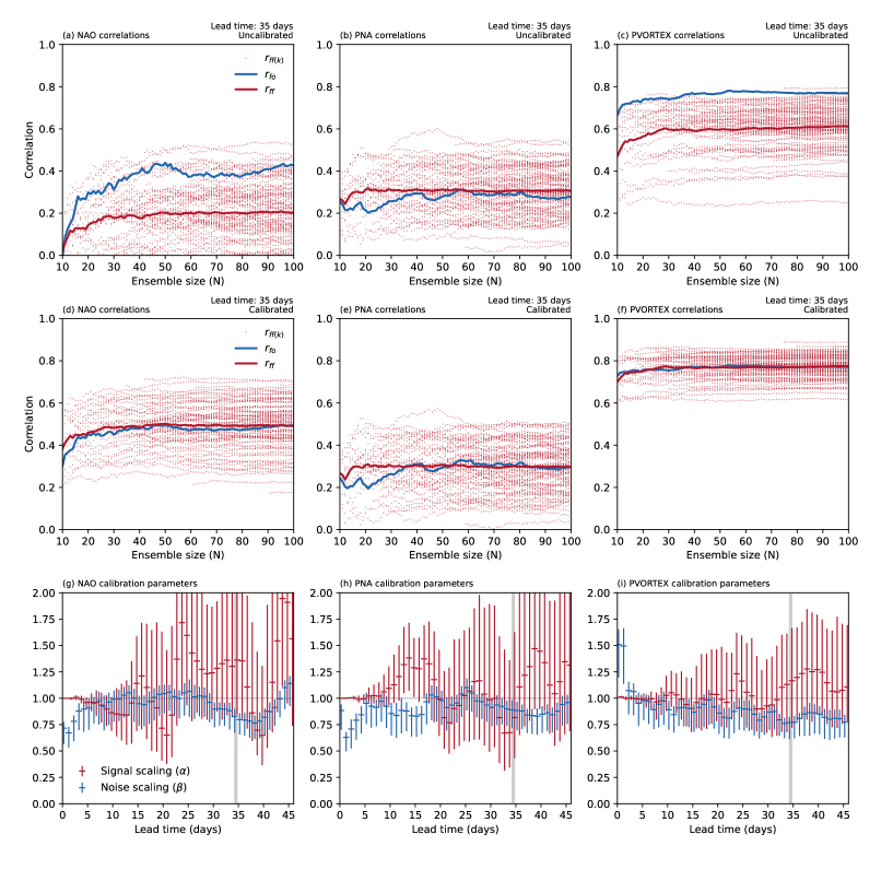
Figure 4: (a-c) Correlations vs ensemble size for circulation indices calculated from uncalibrated forecast anomalies, where $r_{fo}$ is the correlation between the forecast ensemble mean and ERA5, $r_{ff(k)}$ is the correlation between a forecast ensemble mean and an excluded ensemble member, and $r_{ff}$ is the mean of $N+1$ estimates of $r_{ff(k)}$. (d-f) As above, but for indices calibrated using an unbiased member-by-member approach that simultaneously enforces climatological reliability and ensemble variance reliability (see section 3.5). (g-i) Mean of calibration parameters $\alpha$ and $\beta$ (see equations 11 and 12) used in panels d-e. Uncertainties in parameter values are estimated using a bootstrap resampling approach whereby average calibration parameters are calculated 500 times using randomly selected (with replacement) start years. Error bars represent the 2.5th and 97.5th percentiles of the resulting distributions. The vertical grey bar indicates the start date plotted in panels a-f.

Figure 4a-c shows estimates of $r_{ff(k)}$ and $r_{fo}$ for each circulation index at a lead time of 35 days and calculated as a function of ensemble size. From this comparison, it is clear that NAO estimates of $r_{fo}$ lie within the distribution of $r_{ff(k)}$ estimates for all ensemble sizes (figure 4a). For example, NAO indices calculated using $N=99$ members have $r_{fo}=0.43$ and $r_{ff}=0.20$ but estimates of $r_{ff(k)}$ range from -0.15 to 0.52. Based on several lines of evidence, including comparisons of $r_{fo}$ and $r_{ff(k)}$, the unphysical variations in $r_{fo}$ with lead time, and our previous assessment of sampling uncertainties in a perfectly reliable ensemble, we consider the anomalously high values of RPC for NAO indices at subseasonal lead times in these reforecasts to be a consequence of substantial observational sampling uncertainties.

For the same lead time of 35 days, PNA estimates of $r_{fo}$ also lie within the distribution of $r_{ff(k)}$ estimates for all ensemble sizes (figure 4b), which is consistent with the similarity of $r_{fo}$ and $r_{ff}$ across lead times evident in figure 3h. In contrast, PVORTEX estimates of $r_{fo}$ at day 35 either exceed or are very close to the maximum value of $r_{ff(k)}$ for all ensemble sizes (figure 4c). For example, PVORTEX indices calculated with $N=70$ members have $r_{fo}=0.77$ and $r_{ff}=0.60$ but estimates of $r_{ff(k)}$ range from 0.25 to 0.75. In this case, we consider the diagnosed RPC $>1$ to be statistically robust and a consequence of the over-dispersion of PVORTEX forecasts at lead times of more than 25 days.

5 Results for calibrated forecasts

5.1 Direct calibration of circulation indices

This section evaluates the reliability and signal-to-noise characteristics of daily mean NAO, PNA, and PVORTEX indices after application of the unbiased member-by-member calibration described in section 3, which simultaneously enforces the climatological reliability and ensemble variance reliability criteria. The estimated calibration parameters $\alpha$ and $\beta$ modify the ensemble mean (i.e. the predictable signal) and perturbations from the ensemble mean (i.e. the unpredictable noise), respectively. Parameters are estimated separately for each lead time and start month. We do not make any separation between training and verification data when estimating calibration parameters as the intention is to understand the statistical properties of this set of reforecasts rather than optimise the skill of a real-time forecast system.

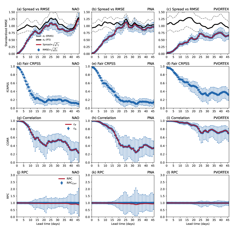
Figure 5: As figure 3, but for calibrated circulation indices.

The results of calibrating each forecast index are summarised in figure 5. As expected, the in-sample reliability calibration enforces the constraints that $\left(\frac{\textnormal{Spread}}{\textnormal{RMSE}}\right)_{\textnormal{unbiased}}=1$ and $\sigma_{z}=\sigma_{T}$ (figure 5a-c). Calibration also modifies $r_{ff}$ to exactly match $r_{fo}$ such that RPC${}_{Corr}=1$ at all lead times in all three circulation indices (figure 5g-i). In spite of the ‘perfect’ RPC values and substantial changes to $r_{ff}$, $\sigma_{z}$, and ensemble spread, calibration has a limited impact on forecast skill diagnosed using RMSE, $r_{fo}$, and CRPSS (figure 5). Furthermore, the ensemble spread of calibrated forecasts no longer increases smoothly and monotonically with lead time as it is forced to inherit the variations with lead time that are present in RMSE. Similarly, estimates of $\sigma_{z}$ and $r_{ff}$ derived from calibrated forecasts also inherit the unphysical variations with lead time that are present in $\sigma_{T}$ and $r_{fo}$, respectively. We conclude that the elimination of an apparent SNP in our calibrated index forecasts is, in part, a consequence of overfitting to the available observations, such that sample statistics from calibrated forecasts inherit the large sampling uncertainties present in the observations.

Figure 4d-f shows estimates $r_{fo}$, $r_{ff}$, and $r_{ff(k)}$ vs ensemble size from calibrated index forecasts for a lead time of 35 days. In a perfectly reliable ensemble, $r_{ff(k)}$ and $r_{fo}$ can be considered drawn from the same underlying probability distribution and their values will converge with $r_{ff}$ when sample statistics are evaluated over many independent start dates (see discussion in section 3.6). However, despite the perfect agreement between $r_{ff}$ and $r_{fo}$ across all lead times (for $N=99$), the calibrated forecasts still exhibit a large spread in estimates of $r_{ff(k)}$ (figure 4d-f). This is inconsistent with our expectations of a perfectly reliable ensemble and is further evidence that the that ‘perfect’ RPC_Corr values in our finite set of forecasts can only be achieved through some degree of overfitting.

Despite the overfitting issues discussed above, it is still instructive to evaluate the calibration parameters $\alpha$ and $\beta$ and their associated uncertainties as a function of lead time (figure 4g-i). Crucially, we find no evidence for statistically robust underestimation of the magnitude of predictable signals (i.e. $\alpha>1$) for any of the three circulation indices. For example, estimates of $\alpha$ for NAO forecasts range between $\sim$0.6 and $\sim$1.9 with large uncertainty estimates that overlap $\alpha=1$ . In contrast, estimates of $\beta$ have much smaller sampling uncertainties with several features that are worthy of comment. Firstly, short-range NAO and PNA forecasts have $\beta<1$, which is indicative of over-dispersion at these lead times. In contrast, short-range PVORTEX forecasts have $\beta>1$, which is indicative of under-dispersion. However, the absolute values of spread are very small at these lead times and thus differences between spread and error are not evident in figure 3a-b. PNA and NAO forecasts also exhibit other periods with $\beta<1$, but these generally correspond to lead times when RMSE and $\sigma_{T}$ are reduced compared to surrounding lead times, which is indicative of observational sampling uncertainty. Lastly, PVORTEX forecasts exhibit a seemingly statistically robust $\beta<1$ at lead times greater than 20 days (figure 4i). This is consistent with the over-dispersion (i.e. spread $>$ RMSE) at lead times greater than 25 days that is associated with RPC $>1$ (figure 3).

5.2 Indirect calibration of circulation indices

We also evaluate the impact of an indirect calibration approach, whereby forecast anomalies are calibrated separately for each grid-point, start month, and lead time prior to calculating forecast indices. This allows us to evaluate both the reliability and signal-to-noise characteristics of the circulation indices together with other aspects of the circulation, such as tropical-extratropical teleconnections.

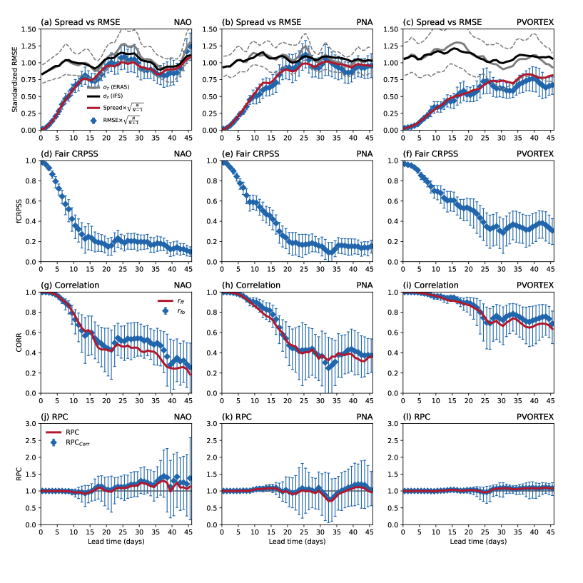
Figure 6: As figure 3, but for circulation indices derived from calibrated grid-point anomalies.

The impact of indirect anomaly calibration (figure 6) is similar, but not identical, to the impact of direct calibration of circulation indices (figure 5). There is improved agreement between both (i) spread and RMSE and (ii) $\sigma_{z}$ and $\sigma_{T}$, which comes at the cost of unphysical variations with lead time as discussed in section 5.1. In addition, there is closer agreement between $r_{ff}$ and $r_{fo}$ such that RPC${}_{Corr}\approx 1$ within our estimated sampling uncertainties at all lead times in all three circulation indices (figure 6g-i). The differences between calibration methods are a consequence of the covariance between grid points, which are not accounted for when calibrating grid-points independently. For example, it is possible for grid points to individually have perfect variances, but the variance of their sum can be incorrect if there are errors in the correlation between grid-points.

In spite of this ‘imperfect’ indirect calibration and the overfitting issues discussed in section 5.1, these calibrated anomalies provide an opportunity to evaluate other properties of the atmospheric circulation in the presence and absence of an apparent SNP. Roberts et al. (2023) recently demonstrated that ECMWF reforecasts with IFS cycle 47R3 accurately simulate wintertime Euro-Atlantic regime structures, frequencies, and transition probabilities, at subseasonal lead times. However, they emphasised that IFS reforecasts underestimate the response of the NAO to the Madden-Julian oscillation (MJO) and fail to reproduce the modulation of MJO-NAO teleconnections by El Niño-Southern Oscillation (ENSO). These conditional errors were attributed to deficiencies in the representation of tropical-extratropical teleconnections, which have been identified in previous IFS cycles and other subseasonal forecast systems (e.g. Vitart, 2017). Importantly, underestimation of tropical-extratropical teleconnection signals such that forecasts do not fully exploit the response of the extratropics to predictable intraseasonal variability in the tropics is one of the proposed physical interpretations for the SNP in seasonal forecasts (Garfinkel et al., 2022; Scaife and Smith, 2018).

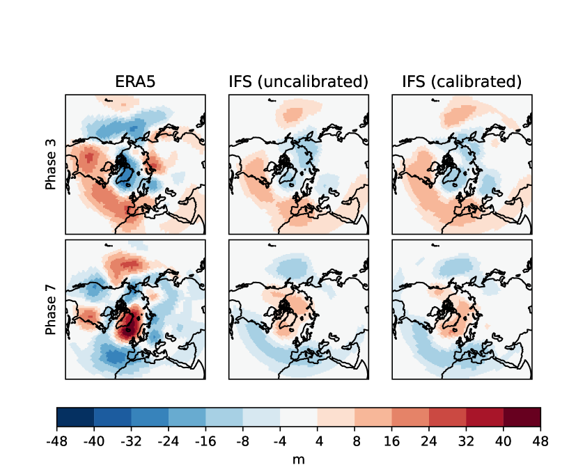
Figure 7: Composite means of 500 hPa geopotential height anomalies based on daily mean ERA5 and IFS reforecast anomalies 15 days after the specified MJO phase. Calibrated composites are constructed using MJO indices derived from forecast anomalies that have been calibrated separately for each grid-point, start month, and lead time as described in section 5.2. Contributing data are selected using the MJO phase calculated separately in each forecast member and weak amplitude events (i.e. $\sqrt{\textnormal{RMM1}^{2}+\textnormal{RMM2}^{2}}<1$) are excluded from the composite calculation. All forecast lead times are considered together (i.e. composite means are constructed from forecast anomalies corresponding to days 16-46 using MJO phases identified during days 1-31). ERA5 data are subsampled to exactly match the available forecast data.

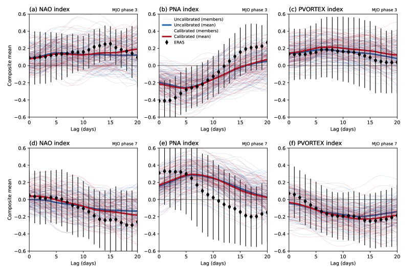
Figure 8: Lagged composites of daily circulation indices (NAO, PNA, PVORTEX) conditioned on the phase of the MJO. As in figure 7, contributing data are selected using the MJO phase calculated separately in each forecast member and weak amplitude events (i.e. $\sqrt{\textnormal{RMM1}^{2}+\textnormal{RMM2}^{2}}<1$) are excluded from the composite calculation. Uncertainties in ERA5 composites are estimated by bootstrap resampling (with replacement) from the available start dates such that error bars represent the 2.5th and 97.5th percentiles of the resulting distribution. Blue and red lines represent composites constructed from uncalibrated and calibrated forecast data, respectively. Calibrated composites are constructed using indices derived from forecast anomalies that have been calibrated separately for each grid-point, start month, and lead time as described in section 5.2. Bold red/blue lines represent composites constructed using 100 forecast members. Thin red/blue lines represent composites constructed using a single member from each forecast start date.

Our evaluation of ERA5 teleconnections (figures 7 and 8) is qualitatively consistent with previous studies that have described the impact of the MJO on the NAO, PNA, and PVORTEX (e.g. Cassou, 2008; Lin et al., 2009; Garfinkel et al., 2012; Seo and Son, 2012; Garfinkel et al., 2014; Barnes et al., 2019; Lee et al., 2019; Wang et al., 2020; Roberts et al., 2023). In particular, ERA5 geopotential height anomalies in the Euro-Atlantic sector that occur 15 days after MJO phases 3 and 7 (figure 7) project onto the positive and negative phases of the NAO, respectively (figure 8). Uncalibrated IFS reforecasts also simulate an NAO response to the MJO, but the lagged composites constructed from 100 forecast members are weaker than estimates based on ERA5 data (figures 7 and 8). However, consistent with our discussion of ERA5-based sample statistics, there is considerable sampling uncertainty in NAO, PNA, and PVORTEX composites constructed from daily data such that 100-member IFS composites are within the 95% confidence limits of ERA5 composites for all indices and MJO phases/lags (figure 8). Similarly, ERA5-based composites lie within the distribution of uncalibrated IFS estimates based on a single member from each forecast start date (figure 8). From this comparison it is clear that more start dates and/or longer composite averaging periods are required to robustly detect differences between IFS and ERA5 MJO teleconnections.

Nevertheless, the important result for this study is that MJO teleconnections are very similar in calibrated and uncalibrated forecasts (figures 7 and 8). The magnitude of the NAO index in the 15-20 days following MJO phase 3/7 is slightly higher in calibrated forecasts, but this difference is small compared to the uncertainty in the ERA5-based composites. In general, the detailed representation of MJO teleconnections in these reforecasts seems to be independent of the presence or absence of an apparent SNP in the underlying index. For example, the largest discrepancy between ERA5 and forecast MJO composites is for the PNA, for which $r_{ff}$ and $r_{fo}$ are generally consistent and thus RPC${}_{\textnormal{Corr}}\approx 1$ for all forecast lead times. We expect improvements in the representation tropical-extratropical teleconnections to be associated with improvements in extratropical skill. However, perfect teleconnections are not a prerequisite for climatological and ensemble variance reliability and thus RPC${}_{\textnormal{Corr}}\approx 1$.

6 Discussion and conclusions

In this study we have emphasised that reliable ensemble forecasts will not exhibit an SNP if sample statistics can be evaluated using a sufficiently large ensemble size ($N$) over a sufficiently large number of independent cases ($M$). However, if $M$ is finite, an apparent SNP will sometimes occur in large ensemble forecasts as a natural consequence of sampling uncertainty, even if forecast members and observations are drawn from the same underlying probability distribution (figure 1). The likelihood of misdiagnosing an SNP is increased when predictability is low and the number of independent forecast start dates are limited (figure 2). Long-range forecasting systems that predict anomalies in seasonal-to-decadal means are particularly vulnerable to this effect due to the modest predictability at longer lead times and limited availability of independent start dates for verification.

In section 4 we evaluated the forecast skill, reliability characteristics, and signal-to-noise properties of three large-scale atmospheric circulation indices in 100-member subseasonal reforecasts. Daily mean NAO and PNA forecasts generally satisfy climatological reliability (equation 3) and ensemble variance reliability (equation 4) criteria within the tolerance of our estimated sampling uncertainties. In contrast, PVORTEX forecasts become significantly over-dispersive (i.e. spread > RMSE) at lead times greater than 25 days (figure 3). Consistent with recent studies, this reforecast dataset exhibits an apparent SNP in the NAO at subseasonal lead times. Based on several lines of evidence, we consider the anomalously high values of RPC for NAO indices at subseasonal lead times in these reforecasts to be a consequence of substantial observational sampling uncertainties, which are common to all model comparisons over the same period. In contrast, we consider the diagnosed RPC $>1$ in PVORTEX forecasts to be statistically robust and a consequence of the over-dispersion of PVORTEX forecasts at lead times of more than 25 days.

In section 5 we demonstrated that the apparent SNP in our reforecast dataset can be eliminated by application of an unbiased member-by-member calibration, which produces ensemble forecasts that exactly satisfy the climatological reliability and unbiased ensemble variance reliability conditions described in section 3.2. However, for the NAO, this is achieved through overfitting such that sample statistics from calibrated forecasts inherit the large sampling uncertainties present in the observations and thus exhibit unphysical variations with lead time. In addition, tropical-extratropical MJO teleconnections are very similar in calibrated and uncalibrated forecasts (7 and 8). The quality of MJO teleconnections in these reforecasts seems to be independent of the presence or absence of an apparent SNP in the underlying index. Based on this evaluation we conclude that improvements in the representation tropical-extratropical teleconnections may be important for future advances in subseasonal forecast skill, but such improvements are not necessarily a prerequisite for reliability or eliminating an apparent SNP in extratropical circulation indices.

Based on the statistical considerations in section 3 and our analysis of large-ensemble subseasonal reforecasts in sections 4 and 5 we make the following recommendations for the robust and unbiased evaluation of reliability and signal-to-noise properties in the presence of large sampling uncertainties:

1. All relevant sample statistics should include uncertainty estimates. Of particular importance is the uncertainty in the observed variance ($\sigma_{T}^{2}$), which is insensitive to ensemble size and can be reduced through the use of longer reforecast periods (e.g. Shi et al., 2015; Weisheimer et al., 2019) and/or more frequent initialization.

2. The optimal (affordable) balance of start dates and ensemble members should be carefully considered when designing (re)forecast datasets to evaluate ensemble reliability and signal-to-noise properties. The reforecast configuration that minimises the chances of misdiagnosing an SNP depends on the intrinsic predictability of the process under investigation (e.g. figure 2). In many situations, an increased number of independent start dates ($M$), which impacts both observation and model sampling uncertainties, could be more useful than increased ensemble size ($N$).

3. Sample statistics (e.g. RMSE, spread, variance) should be calculated using unbiased estimators that account for the systematic effects of ensemble size and, in the case of anomalies, the sample size of the reference climatology (Leutbecher and Palmer, 2008; Roberts and Leutbecher, 2024). A simple approach to ensure that anomaly-based statistics are unbiased with respect to climatology sample size is to construct forecast anomalies separately for each member (Roberts and Leutbecher, 2024). This approach has no impact on ensemble means, but ensures that forecast member anomalies remain statistically exchangeable with observed anomalies if the underlying raw forecasts are perfectly reliable. This method of anomaly calculation does not affect estimates of r_fo but impacts estimates of ensemble spread, total anomaly variance, r_ff(k), and r_ff. The ensemble size and reforecast sample size effects are small for the 100-member and 20-year reforecasts considered in this study. However, they may not be negligible when considering smaller ensemble sizes and/or shorter reforecast periods.

4. The observation-based ($r_{fo}$) and model-based ($r_{ff(k)}$) correlations used to define RPC_Corr should be calculated such they are statistically exchangeable in the limit of a perfectly reliable ensemble (section 3.3). For example, model-based correlations should be calculated between the ensemble mean and an excluded member and observation-based correlations should use an ensemble size of N-1 to match the model-based correlations. For small ensemble sizes, calculating $r_{fo}$ with $N$ members and $r_{ff(k)}$ with $N-1$ members could lead to misdiagnosis of an SNP.

5. Statistically robust diagnosis of an SNP should include demonstration that $r_{fo}$ does not plausibly lie within the distribution of estimates of $r_{ff(k)}$. In section 3 we emphasised that a perfectly reliable ensemble, in which forecasts and observations are drawn from the same probability distribution at each start date, can still exhibit RPC${}_{Corr}>1$ and thus an apparent predictability paradox when evaluated using a finite number of start dates ($M$). Crucially, $r_{ff}$ represents the mean of $N$ estimates of $r_{ff(k)}$ and thus has a much smaller sampling uncertainty such that $r_{fo}$ and $r_{ff}$ are not generally statistically exchangeable, even in a perfectly reliable ensemble.

6. If possible, forecast skill and other sample statistics should be evaluated over a range of lead times. When averaged over a sufficiently large number of cases, forecast errors and their proxies (e.g. ensemble spread) should grow monotonically before saturating at the intrinsic predictability limit. Predictability paradoxes that emerge at particular lead times due to spurious reductions in forecast error associated with observational sampling uncertainties should be treated with suspicion.

7. Unbiased reliability calibration can be used for attribution of an apparent SNP to either weak predictable signals (i.e. $\alpha>1$) and/or overestimated unpredictable noise (i.e. $\beta<1$). However, such methods are vulnerable to overfitting to the available observational data and should be accompanied by uncertainty estimates for the derived calibration parameters.

We encourage researchers to apply these principles when assessing ensemble reliability and signal-to-noise properties in other ensemble forecast systems to avoid misinterpreting the impacts of sampling uncertainty. Although we have concluded that an apparent SNP in the subseasonal NAO forecasts presented in this study are a consequence of observational sampling uncertainties, other studies considering different forecast systems, lead times, or indices may find a statistically robust difference between $r_{fo}$ and $r_{ff(k)}$ such that there is confidence that RPC $>1$. However, such forecasts are by definition also unreliable, either because the predictable signal is too weak (i.e. $\alpha>1$) or the unpredictable noise is too large (i.e. $\beta<1$). Whether such unreliability represents a predictability ‘paradox’ is then a matter of perspective. Crucially, this means there is no inconsistency between the objectives of eliminating a signal-to-noise paradox and traditional approaches to ensemble forecast development guided by unbiased evaluation of forecast reliability and optimization of fair ensemble scores (e.g. Ferro, 2014).

Conflict of interest

The authors declare no conflict of interest.

References

- Baker et al. (2018) Baker, L., Shaffrey, L., Sutton, R., Weisheimer, A. and Scaife, A. (2018) An intercomparison of skill and overconfidence/underconfidence of the wintertime North Atlantic Oscillation in multimodel seasonal forecasts. Geophysical Research Letters, 45, 7808–7817.
- Baldwin and Dunkerton (1999) Baldwin, M. P. and Dunkerton, T. J. (1999) Propagation of the Arctic Oscillation from the stratosphere to the troposphere. Journal of Geophysical Research: Atmospheres, 104, 30937–30946.
- Barnes et al. (2019) Barnes, E. A., Samarasinghe, S. M., Ebert-Uphoff, I. and Furtado, J. C. (2019) Tropospheric and stratospheric causal pathways between the MJO and NAO. Journal of Geophysical Research: Atmospheres, 124, 9356–9371.
- Bröcker et al. (2023) Bröcker, J., Charlton-Perez, A. J. and Weisheimer, A. (2023) A statistical perspective on the signal-to-noise paradox. Quarterly Journal of the Royal Meteorological Society, 149, 911–923.
- Cassou (2008) Cassou, C. (2008) Intraseasonal interaction between the Madden–Julian oscillation and the North Atlantic Oscillation. Nature, 455, 523–527.
- Dawson (2016) Dawson, A. (2016) eofs: A library for EOF analysis of meteorological, oceanographic, and climate data. Journal of Open Research Software, 4.
- Dee et al. (2011) Dee, D. P., Uppala, S. M., Simmons, A. J., Berrisford, P., Poli, P., Kobayashi, S., Andrae, U., Balmaseda, M., Balsamo, G., Bauer, d. P. et al. (2011) The ERA-Interim reanalysis: Configuration and performance of the data assimilation system. Quarterly Journal of the royal meteorological society, 137, 553–597.
- Doblas-Reyes et al. (2009) Doblas-Reyes, F., Weisheimer, A., Déqué, M., Keenlyside, N., McVean, M., Murphy, J., Rogel, P., Smith, D. and Palmer, T. (2009) Addressing model uncertainty in seasonal and annual dynamical ensemble forecasts. Quarterly Journal of the Royal Meteorological Society: A journal of the atmospheric sciences, applied meteorology and physical oceanography, 135, 1538–1559.
- Eade et al. (2014) Eade, R., Smith, D., Scaife, A., Wallace, E., Dunstone, N., Hermanson, L. and Robinson, N. (2014) Do seasonal-to-decadal climate predictions underestimate the predictability of the real world? Geophysical research letters, 41, 5620–5628.
- Ferro (2014) Ferro, C. (2014) Fair scores for ensemble forecasts. Quarterly Journal of the Royal Meteorological Society, 140, 1917–1923.
- Garfinkel et al. (2014) Garfinkel, C. I., Benedict, J. J. and Maloney, E. D. (2014) Impact of the MJO on the boreal winter extratropical circulation. Geophysical Research Letters, 41, 6055–6062.
- Garfinkel et al. (2022) Garfinkel, C. I., Chen, W., Li, Y., Schwartz, C., Yadav, P. and Domeisen, D. (2022) The winter North Pacific teleconnection in response to ENSO and the MJO in operational subseasonal forecasting models is too weak. Journal of Climate, 35, 8013–8030.
- Garfinkel et al. (2012) Garfinkel, C. I., Feldstein, S. B., Waugh, D. W., Yoo, C. and Lee, S. (2012) Observed connection between stratospheric sudden warmings and the Madden-Julian Oscillation. Geophysical Research Letters, 39.
- Garfinkel et al. (2024) Garfinkel, C. I., Knight, J., Taguchi, M., Schwartz, C., Cohen, J., Chen, W., Butler, A. H. and Domeisen, D. I. (2024) Development of the signal-to-noise paradox in subseasonal forecasting models: When? Where? Why? Quarterly Journal of the Royal Meteorological Society.
- Gottschalck et al. (2010) Gottschalck, J., Wheeler, M., Weickmann, K., Vitart, F., Savage, N., Lin, H., Hendon, H., Waliser, D., Sperber, K., Prestrelo, C. et al. (2010) A framework for assessing operational model MJO forecasts: a project of the CLIVAR Madden-Julian oscillation working group. Bull Am Meteorol Soc, 91, 1247–1258.
- Hardiman et al. (2022) Hardiman, S. C., Dunstone, N. J., Scaife, A. A., Smith, D. M., Comer, R., Nie, Y. and Ren, H.-L. (2022) Missing eddy feedback may explain weak signal-to-noise ratios in climate predictions. npj Climate and Atmospheric Science, 5, 57.
- Hersbach et al. (2020) Hersbach, H., Bell, B., Berrisford, P., Hirahara, S., Horányi, A., Muñoz-Sabater, J., Nicolas, J., Peubey, C., Radu, R., Schepers, D. et al. (2020) The ERA5 global reanalysis. Quarterly Journal of the Royal Meteorological Society, 146, 1999–2049.
- Hopson (2014) Hopson, T. (2014) Assessing the ensemble spread–error relationship. Monthly Weather Review, 142, 1125–1142.
- Hoskins and Karoly (1981) Hoskins, B. J. and Karoly, D. J. (1981) The steady linear response of a spherical atmosphere to thermal and orographic forcing. Journal of the atmospheric sciences, 38, 1179–1196.
- Hurrell (1995) Hurrell, J. W. (1995) Decadal trends in the North Atlantic Oscillation: Regional temperatures and precipitation. Science, 269, 676–679.
- Ineson and Scaife (2009) Ineson, S. and Scaife, A. (2009) The role of the stratosphere in the European climate response to El Niño. Nature Geoscience, 2, 32–36.