Machine Learning and Multi-source Remote Sensing
in Forest Carbon Stock Estimation:
A Review

Abstract

Quantifying forest carbon is crucial for informing decisions and policies that will protect the planet. Machine learning (ML) and remote sensing (RS) techniques have been used to do this task more effectively, yet there lacks a systematic review on the most recent ML methods and RS combinations, especially with the consideration of forest characteristics. This study systematically analyzed 25 papers meeting strict inclusion criteria from over 80 related studies, identifying 28 ML methods and key combinations of RS data. Random Forest had the most frequently appearance (88% of studies), while Extreme Gradient Boosting showed superior performance in 75% of the studies in which it was compared with other methods. Sentinel-1 emerged as the most utilized remote sensing source, with multi-sensor approaches (e.g., Sentinel-1, Sentinel-2, and LiDAR) proving especially effective. Our findings provide grounds for recommending best practices in integrating machine learning and remote sensing for accurate and scalable forest carbon stock estimation.

Machine Learning and Multi-source Remote Sensing
in Forest Carbon Stock Estimation: A Review
Autumn Nguyen^*, Sulagna Saha
Mount Holyoke College
^*Corresponding author: ngoc54n@mtholyoke.edu

1 Introduction

1.1 Why forests carbon stock estimation?

Forests capture carbon, which helps regulate climate. The main driver of the increasing global deforestation is because forests are mostly valued in terms of their economical value, like how much timber or area of land they can provide, rather than on how much they help regulate climate. To quantify the value of forests in fighting climate change consequences, we need to quantify forests’ carbon stock.

1.2 How does forest carbon get measured?

The best way to measure the amount of carbon sequestered in a forest is to do so with direct field measurements (Cunningham and Montgomery 2011). People go into the forest to count the trees, measure the trees’ DBH, measure canopy height, identify species, etc. Those data would be put into forestry allometric equations to calculate the forests’ aboveground biomass (AGB). Belowground biomass (BGB) and soil organic carbon are other key components of forests’ total biomass, but it cannot be quantified well from remote sensing data. “Due to the difficulty of collecting field survey data of belowground biomass, the majority of previous biomass studies have focused on AGB.” (Lu et al. 2016). Most of the papers reviewed in this paper were also estimations of AGB.

The role of forests in countering the climate crisis is not only in sequestering and storing carbon. The biodiversity that it protects, the soil that it keeps from eroding, the rainwater that it keeps from becoming flood, the pollutants that it removes from the atmosphere… are just a few of the important gifts that forests give to the Earth.

	Passive optical	Active optical	Radar (SAR)
Examples	Sentinel-2 MODIS Landsat	LiDAR	Sentinel-1 ALOS-PALSAR
Capabilities	Widely and freely available High resolution	Able to measure 3D structural data Can work at nighttime High resolution	Can penetrate dense canopies and clouds Can work at nighttime
Limitations	Cannot work at nighttime Cannot penetrate dense canopies or clouds	Expensive Available in only certain small areas	Lower resolution than optical Saturation issues

Table 1: Capabilities and limitations of most common categories of remote sensing technologies

1.3 Why remote sensing?

1.3.1 Because carbon stock estimation no longer feasible with traditional inventory

It requires too much personnel and equipment and takes too much time for field measurements to be feasible to measure carbon stocks of large forest areas. Moreover, it is still impossible to go into some deep forest areas to take measurements, at least if we don’t want to cause disturbances in nature.

1.3.2 What can remote sensing offer

By their ability to fly over large areas with minimal disturbance, remote sensing technologies can capture information about large-scale forests, such as tree density, vegetation cover, and 3D structures, and these data are closely related to AGB. According to (Cunningham and Montgomery 2011), “remote sensing is a general term describing the technology and application for observing the earth. Glamorous technologies include satellite imaging, but remote sensing also includes traditional aerial photography. Remote sensing technology is not only used to make accurate maps and measurements of forests, but more sophisticated sensors utilizing LiDAR (Light Detection and Ranging) and SAR (Synthetic Aperture Radar) can be used to quantify the biomass content of a forest.”

1.3.3 Perks and key issues of remote sensing-based models

(Lu et al. 2016) said that previous research had shown that remote sensing-based models provide more accurate biomass estimation than other models (e.g. process-based ecosystem models, GIS-based empirical models…). However, the assumption that must be made when using remote sensing-based methods was that forest stand information captured by sensors was highly correlated with aboveground biomass (Lu et al. 2012). Therefore, we needed to ensure a sufficient number of available sample plots, suitable metrics selected for modeling, suitable algorithms used to establish the models, and suitable methods used to conduct uncertainty analysis of the estimates (Lu et al. 2012).

1.4 Why multi-source remote sensing?

In short, combining multiple sources remote sensing is promising because it allows the capabilities of one source to compensate for the limitations of the other sources. Examples of a few major categories are collected from studies like (Huang et al. 2022) and summarized in Table 1.

1.5 Why Machine Learning (ML)?

ML are algorithms that can learn from the carbon stock measurements we have for some forest areas to make predictions of what those may be in other forest areas. They can also help with data imputation—which means estimating missing values based on patterns in the data and making the dataset complete for further analysis. An example (Rolnick et al. 2022) gave was ”The height of trees can be estimated fairly accurately with LiDAR devices mounted on UAVs, but this technology is not scalable and many areas are closed to UAVs. To address this challenge, ML can be used to predict LiDAR’s outcome from satellite imagery. From there, the learned estimator can perform predictions at scale. Despite progress in this area, there is still significant room for improvement.”

1.6 Related studies

(Sun and Liu 2020) did a comprehensive review on the fundamental types of forest carbon estimation: vegetation carbon storage, soil carbon storage, and litter carbon storage. For vegetation carbon storage, Sun found that inventory-based methods were used most often, followed by satellite-based and then process-based methods. Within satellite-based methods, optical remote sensors were used 58 times, while radar sensors were only used once, and LiDAR used 7 times. Our results (4) found radar and LiDAR used much more often than this finding. In addition, our study also reviewed studies globally and reviewed the studies that used ML, while (Sun and Liu 2020) only reviewed the studies in China, and they also did not review the machine learning methods used.

(Rolnick et al. 2022) was a comprehensive big-picture review of ML in climate change-related research and industry efforts. They mentioned the opportunity for ML to help in forest carbon stock estimation, but they had very few references to research studies – many references were either very dated or were blog posts of companies in industry. We focused more on recent academic research in this review paper.

(Hamedianfar et al. 2022) reviewed all deep learning methods used in creating forest inventory. In reviewing the studies related to continuous forest variable estimation, they collected information like the deep learning methods, the ML task (e.g. regression, segmentation, classification, etc.), the data (e.g. LiDAR, Landsat, etc.), the variable (e.g. AGB, canopy height, species, etc.), the sample size (i.e. how many plots), etc. In reviewing the studies related to segmentation and classification, they also collected information like the optimizer, the learning rate, the labeled data, etc. We personally thought this was a very technical paper that would be hard for people without advanced deep learning expertise to understand; thus, one of our aims for our paper is to make the information more accessible to the general audience. In addition, (Hamedianfar et al. 2022) did not cover non-deep learning techniques, which have been used very frequently in forest carbon estimation; and many studies they reviewed stopped at creating forest inventory, without doing any carbon stock estimation using those inventory information.

The most similar review with ours that we could find was (Matiza et al. 2023) on ML and remote sensing approaches in estimating carbon storage in natural forests. They found out that 36% of the studies used more than one type of dataset; however, they did not review the combinations of those different data sources and types, as we aimed to do in this paper. They also did not consider the types or characteristics of the forests studied. Moreover, the studies they reviewed stopped at 2022, and with the increasing number of studies every year in this field (Sun and Liu 2020), we wanted to find the most recent trends by reviewing studies up to 2024.

2 Methods

2.1 Literature search terms

The 25 papers in that we drew quantitative results from were selected from the first 15 results of these search terms: “(estimation OR estimating OR ”machine learning”) (multisource OR multi-source) forest carbon biomass map”, and the first 20 results of these search terms “(estimation OR estimating OR ”machine learning”) (multisensor OR multi-sensor) forest carbon biomass map”. The aim of this search term was to find papers that surely had a Machine Learning component, used a combination of different sources of remote sensing data, and for the purpose of mapping carbon stick or biomass of forests. The reasons for the specific words in the search term are:

• Through our pilot analysis, we noticed that a lot of studies using Machine Learning to estimate forest carbon had words in the family of “estimation” in the title, while “Machine Learning” might not be in the title or even the abstract because the authors just directly used the name of the ML methods.

• Studies that use a combination of active and passive remote sensors usually mentioned “multi-source” or “multi-sensor” explicitly in their title or abstract. “Multi-source” means getting data from multiple different sources, which can be different things than remote sensors (for example, from traditional inventory sources), while “multi-sensor” only refers to using multiple remote sensors. However, since most of the papers we reviewed also used data from multiple remote sensors, we chose to focus on the multi-remote sensing part of multi-source. Having “multi-sensor” instead of “multi-source” in the search term also resulted in a bit more geographical diversity in the sources and study areas of the resulting papers.

• All of the words “forest”, “carbon” “biomass”, and “map” should have frequent presence in the title or abstract to ensure the relevance of the studies to our review topic.

2.2 Literature querying method

We retrieved the papers from this search into a database using the public API from (Ankit 2021), specifically the google_scholar_internal function.

2.3 Inclusion criteria

The 25 papers were included because only them satisfied five of our inclusion criteria: (1) full paper accessible to us (so most are open access articles, since we are college students with almost no subscriptions to any journals), (2) used ML in the study, (3) used multiple sources of remote sensing data, (4) had the end goal being estimation forest carbon, whether it was AGB or BGB or soil carbon, and (5) was written in the recent 10 years (2014-2024).

2.4 Data collection

From the included 25 papers, the following data was collected for the quantitative database:

• All the remote sensing sources that the study took data from.

• All the ML methods used in the study.

• If the study used multiple ML methods for comparison of performance on the same task, or for each method to be used on a different task.

• If the study used multiple ML methods for comparison, which method(s) were found to have the best performance? Since there are many different ways to define ”best”, we just included the methods that were explicitly mentioned in the abstract or conclusion with a keyword ”best”, or ”highest” for metrics like $R^{2}$ or accuracy, or ”lowest” for metrics like RMSE or uncertainty.

• Any limitations or future steps thoroughly explained.

• The ultimate task, such as AGB map, BGB map, general biomass map, multi-scale biomass maps, uncertainty estimation, etc.

• The location(s) of the studied forests.

• The types or characteristics or dominant species of the forests.

  The forest type categories we used in our review are not at all mutually exclusive or deterministic — they are meant to facilitate readers in identifying the papers that work on forests of similar types to their interest.

  Since the words people used to describe their forests varied widely between papers, and there are no world-wide standardized terminologies for either forest types or biomes, we did our best to identify the common terms used across papers, and refer to a few sources ((Xu et al. 2022), (ArcGIS 2024)) to determine the forest types of the papers that did not use exactly those common terms (so we related their terms to the common terms), and of the papers that did not have any terms about the type of their forest (for those, we used the geographical latitude and longitude of the area to determine the type based on the external sources cited above).

• The scale of the study: region, country, or global.

2.5 Data analysis

Python libraries, namely Pandas, Matplotlib, Seaborn, and NumPy, were used to manipulate and visualize data.

3 Results

Study	Data sources	ML methods used
(Fararoda et al. 2021)	ALOS-PALSAR, DEM, MODIS	RF, kNN
(Zhu et al. 2020)	ALOS-PALSAR, Landsat	MLR, RF
(Hong et al. 2023)	Airborne LiDAR, Optical GF-1/PMS1	LSTM, MLR, RF, SVM
(Wang et al. 2022)	ALOS-PALSAR, GLAS/ICESat LiDAR (spaceborne), MODIS	LR, QRNN, RF, SVM, Stepwise LR
(Zhang et al. 2019)	GLAS/ICESat LiDAR (spaceborne), Landsat, MODIS	CubistRegrTree
(Zhang et al. 2022)	ALOS-PALSAR, Sentinel-1, Sentinel-2	CNN, Keras, MLR, RF, SVM
(Tang et al. 2022)	GLAS/ICESat LiDAR (spaceborne), MODIS, SRTM	CatBoost, GBM, LGBM, RF, XGB
(Ehlers et al. 2022)	Airborne LiDAR, Landsat, RaDAR, Sentinel-1	RF
(Hu et al. 2020)	GLAS/ICESat LiDAR (spaceborne), MODIS	RF
(Huang et al. 2023)	DEM, Landsat, Sentinel-2	BayesRegNN, GBM, QRF, RF, RRF, kNN
(Ometto et al. 2023)	ALOS-PALSAR, Airborne LiDAR, MODIS, SRTM	RF
(Ghosh and Behera 2018)	Sentinel-1, Sentinel-2	RF, SGB
(Bispo et al. 2020)	ALOS-PALSAR, Airborne LiDAR, Landsat	RF
(Pötzschner et al. 2022)	GLAS/ICESat LiDAR (spaceborne), MODIS, Sentinel-1	GBM
(Singh et al. 2024)	Sentinel-1, Sentinel-2	ANN, RF, SVM
(Ronoud et al. 2021)	Landsat, Sentinel-1, Sentinel-2	MLR, RF, SVR, kNN
(Qadeer et al. 2024)	DEM, GEDI LiDAR (spaceborne), Sentinel-1, Sentinel-2	CatBoost, GTB, LGBM, RF, XGB
(Chen et al. 2022)	GEDI LiDAR (spaceborne), GLAS/ICESat LiDAR (spaceborne), Sentinel-1, Sentinel-2	RF
(Musthafa and Singh 2022)	ALOS-PALSAR, GEDI LiDAR (spaceborne), Radarsat-2	RF
(Li et al. 2021)	DEM, GF-2 multispectral, Sentinel-2	RFStacking
(Sainuddin et al. 2024)	GEDI LiDAR (spaceborne), SRTM, Sentinel-1, Sentinel-2	BRT, RF, XGB
(Zhang et al. 2020)	GLAS/ICESat LiDAR (spaceborne), GLASS LAI, Landsat, MODIS	ANN, CatBoost, ERT, GBRT, MARS, RF, SGB, SVR
(Ghosh et al. 2022)	ALOS-PALSAR, GEDI LiDAR (spaceborne), Landsat, SRTM, Sentinel-1, Sentinel-2	RF
(Li et al. 2020)	Landsat, Sentinel-1	LR, RF, XGB

Table 2: Data sources and ML methods used in selected studies.

Table 2 was a summary of the data sources and ML methods used in the studies from which quantitative results were drawn from. This is a link to the interactive and prettier-looking version of the database that everyone can filter by forest types, data sources, ML methods, or any keywords they want.

The full names of the abbreviations of the ML methods and data sources can be found in the Appendix.

3.1 ML

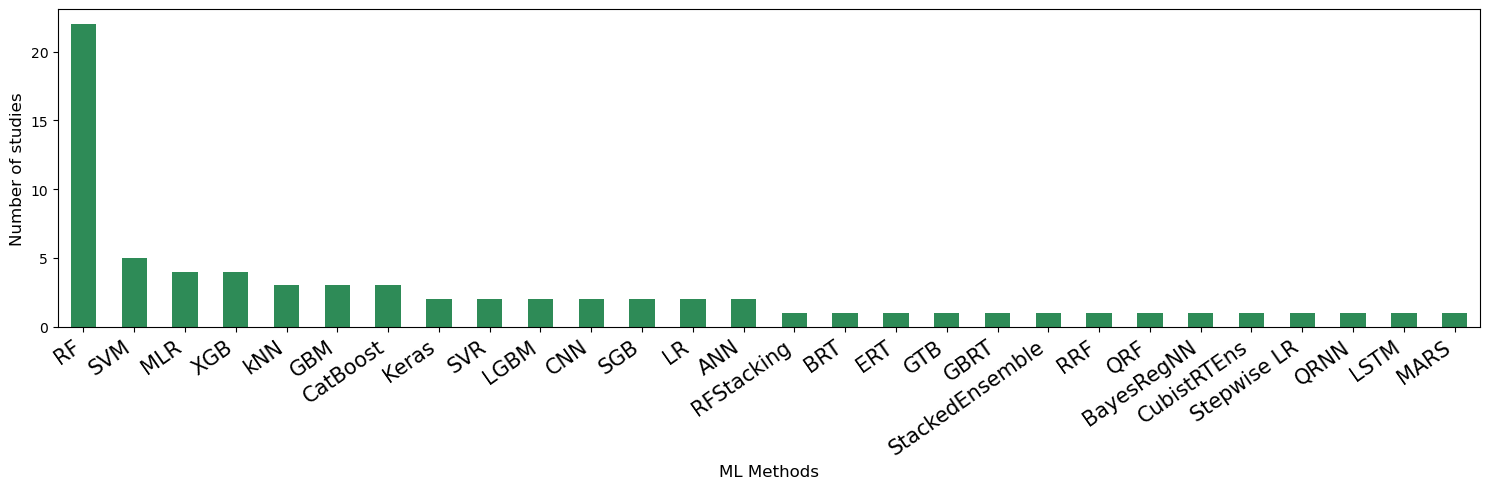
Figure 1: Frequency of ML methods used

Figure 1 shows that RF was used most often – in around 88% of the studies. It was usually used as the model for the end task—AGB estimation, and sometimes as the model for other intermediate tasks in the data processing pipeline.

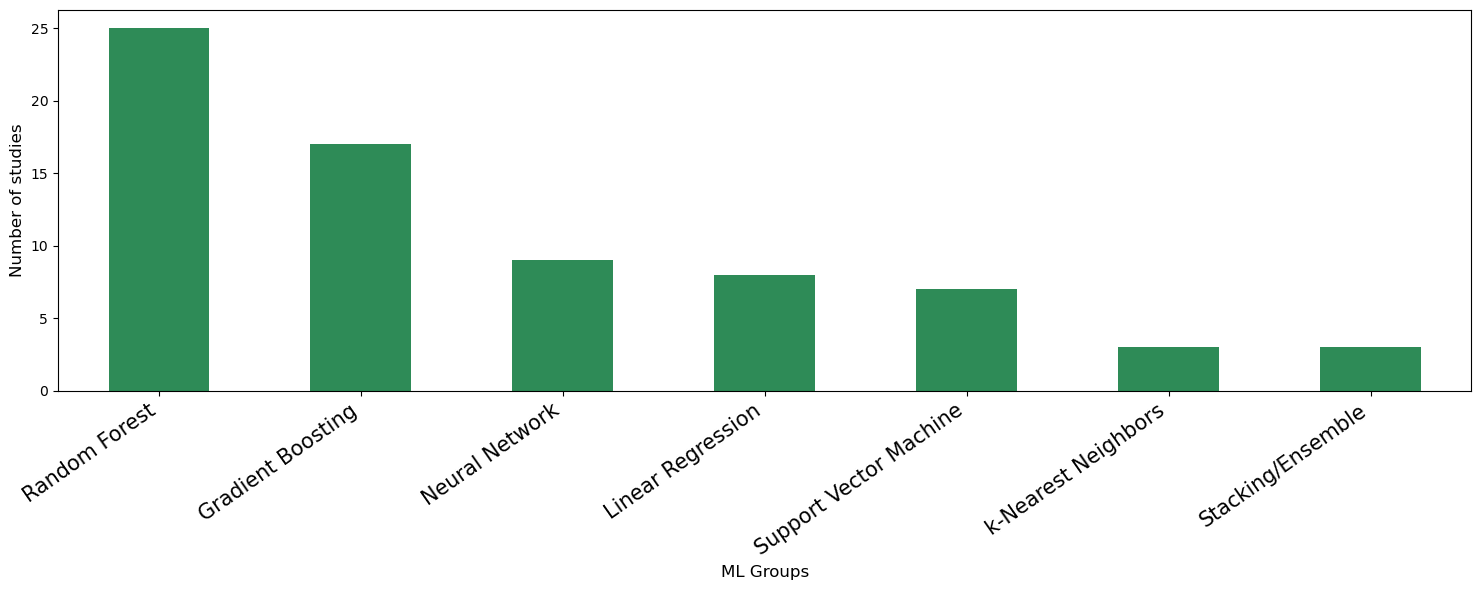
Figure 2: Frequency of ML methods by Groups

Since many of those ML methods are closely related to each other, we grouped them in Figure 2 to see the trend in a bigger picture. Individual members of the groups are specified in the appendix. Random Forests are still the most commonly used methods, but the distribution is more smooth. Most methods found to have the best performance in Figure 3 also fall into the three most frequently used groups: Random Forest (RF, QRF, RRF), Gradient Boosting (XGB, LGBM, CatBoost), and Neural Network (CNN, BayesResNN).

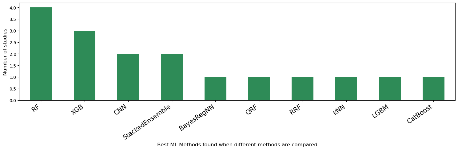
Figure 3: Best ML methods found in studies that compared multiple methods

11 out of 25 studies compared multiple ML methods for the AGB estimation task, and found the model(s) that performed best. While in Figure 3, RF was also the most frequent method, XGB had a higher ”success rate” (which means the ratio of how often it was found to best over how often it was used in total). RF was part of all the studies that compared multiple MLs, but was only found to be best in 4 — which were when RF was compared to regression (LR and MLR), SVM, and neural network (QRNN and ANN). XGB was only used in 4 studies, but was found to perform the best in 3.

• In (Qadeer et al. 2024) study, all gradient boosters (GTB, CatBoost, LightGBM, XGB) had higher $R^{2}$ and less overestimation-underestimation issue compared to RF. The differences between the different kinds of boosters were smaller than the differences between the boosters and RF; XGB had the best $R^{2}$ on Sentinel-2 data, and second-best on Sentinel-1 data and the fused Sentinel-1 and -2 data. Nonetheless, the final AGB map was made using an ensemble of all boosters and RF, so that the strengths and biases of the models were averaged out.

• In (Sainuddin et al. 2024) study, XGB has highest $R^{2}$ compared to RF and Boosted Regression Tree.

• In(Li et al. 2020) study, XGB has best estimations of AGB in high and low range values, while XGB, RF, LR perform similarly in medium range, so XGB also improved the overestimation-underestimation issue.

• In (Tang et al. 2022) study, the best model found was the stack of all the individual models they experimented with, namely RF, GB, XGB, LGBM, and CatBoost — which were exactly the same with those used in the Pakistan study, but they didn’t focus on comparing individual models as in the Pakistan study. However, this one found that XGB had the highest uncertainty.

All these studies were after 2020, which made sense because the rise in popularity of XGB was much more recent compared to RF.

3.2 Remote sensing data sources

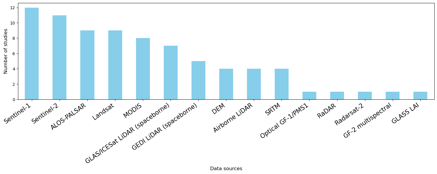
Figure 4: Frequency of data sources used

The most frequently used data source was Sentinel-1, followed by Sentinel-2, ALOS-PALSAR, Landsat, MODIS, GLAS/ICESat LiDAR, and GEDI LiDAR. However, since GLAS/ICESat and GEDI are both spaceborne LiDAR, we can also say that spaceborne LiDARs were the most frequently used source. In (Matiza et al. 2023), which reviewed studies using ML and remote sensing in general globally up till 2022, Landsat was found to be the most frequently used sensor, while Sentinel-1 was the 7th and ALOS-PALSAR was the 13th.

When looking at those sources by types, the most commonly used radar sensors were Sentinel-1 and PALSAR. The most commonly used passive optical sensors were Sentinel-2, Landsat, and MODIS. Spaceborne LiDAR were used more often than airborne LiDAR. Data related to elevation or height (DEM or SRTM) were also used often.

3.3 Combinations of data sources

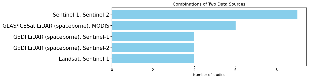
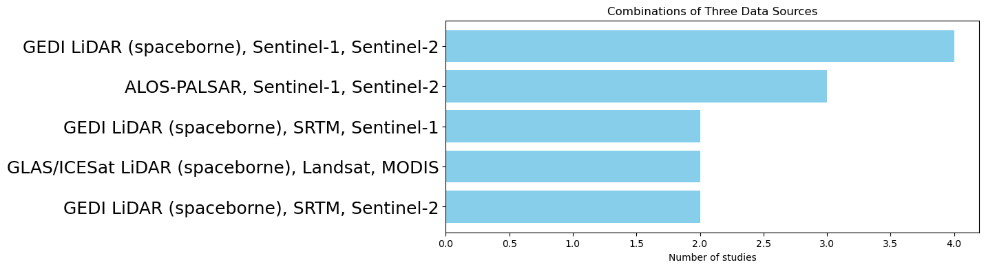
Figure 5: Most common combinations of data sources

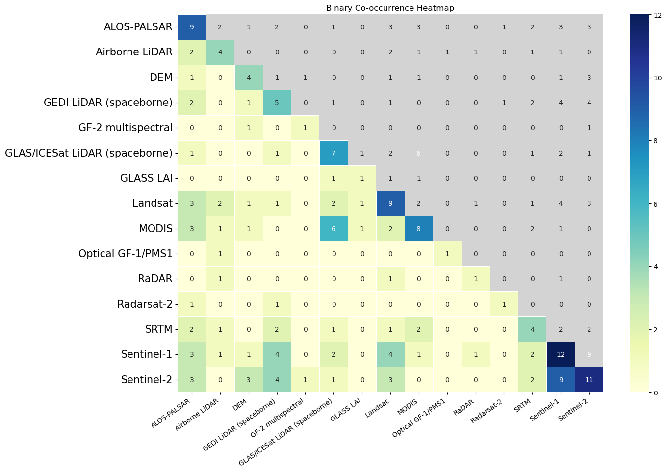
Figure 6: Heatmap: binary co-occurrence of two data sources

From the heatmap 6 and the bar charts 5, it is clear that Sentinel-1, Sentinel-2, and spaceborne LiDAR (GEDI) were most often used together. They made a combination of passive optical, active optical, and radar, complementing each other’s strengths and limitations as described in the Introduction. LiDAR had very limited availability and high costs, so when it was not available, combinations of passive optical and radar also used well together quite often. For example, Landsat and Sentinel-1, or MODIS and Sentinel-2, or MODIS and PALSAR. Nonetheless, some of those studies that used only passive optical and radar sensors faced a common issue of saturation, and LiDAR was usually the recommended solution to that issue.

We can see from the heatmap that when a study used Sentinel-2, they’d likely also include LiDAR or DEM. This is likely because Sentinel-2 is a passive optical sensor with no ability to infer canopy height, an important variable in estimating AGB, and LiDAR or DEM can provide that information..

3.4 Forest types/characteristics

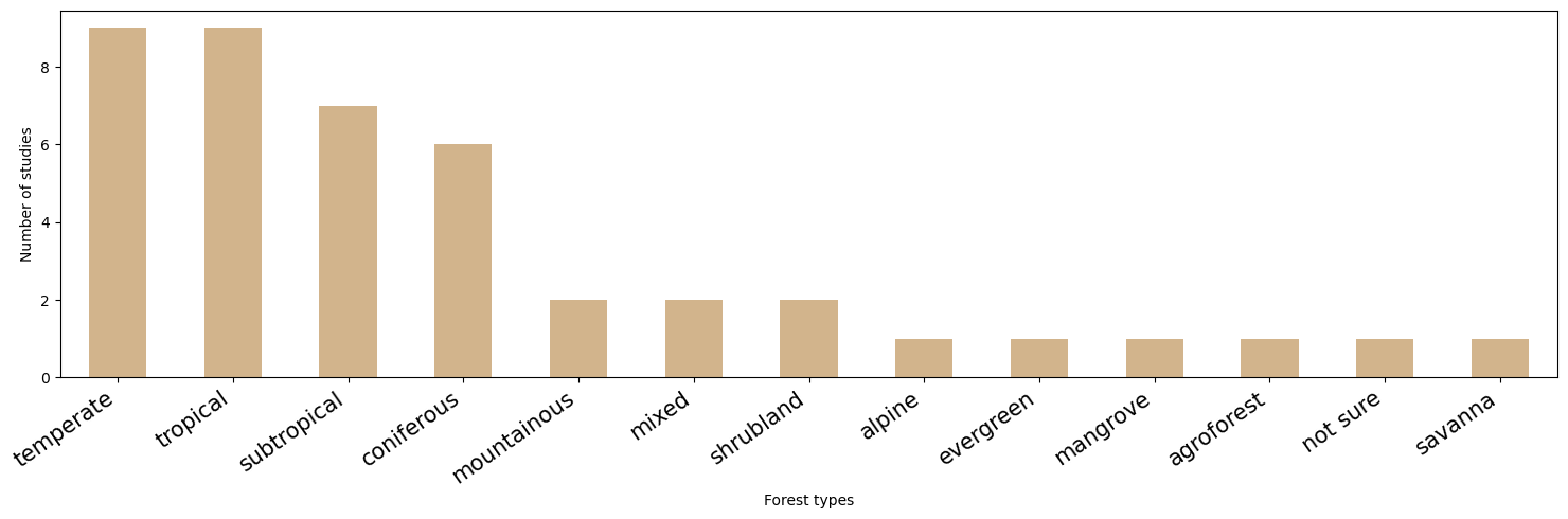
Figure 7: Frequency of forest types studied

In Figure 7, the most frequently studied forests were temperate forests, tropical forests, subtropical forests, and coniferous forests.

3.5 Geographical locations

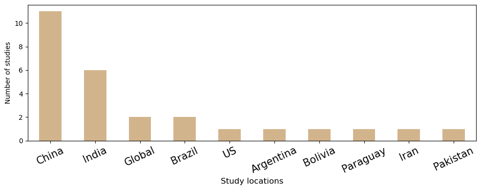
Figure 8: Frequency of geographical locations of the studied forests

China made up around half of the locations of the studies, making it the most frequently appeared country in Figure 8. Since none of the terms were China-related, and all papers were selected from the first-appeared results on Google Scholar rather than from related papers, this may point to some interesting geographical trend of research in the field.

4 Discussion

4.1 Feature selection

4.1.1 General

Feature selection was found to be a critical factor influencing the models’ performances in many studies. Feature selection means selectively choosing which variables, from all the data available, to use as inputs to the estimation models. (Li et al. 2019) demonstrated how variable selection had significantly influenced the performance of all of their models; their XGBoost model was the one benefiting the most from optimal variable selection. (Huang et al. 2022) selected only 7 variables from over 30 initial numerical parameters to use in all of their four data schemes; the Least Absolute Shrinkage and Selection Operator (Lasso) algorithm was used to do feature selection, which they concluded to have been able to “effectively remove the non-significant variables”. However, there were studies that did not do variable selection, like (Li et al. 2020). Their main reason was that their dataset didn’t have a lot of variables, and their Sentinel variables might all be lost after multiple rounds of variable selections. Since their main goal was to compare the performance of the models between a single sensor dataset and multi-sensors combined dataset, they couldn’t afford to lose all variables in their Sentinel dataset. Another reason they gave was that their ML models were robust against noise: the RF algorithm was not influenced by noisy variables; the XGB model, though not as resistant as RF, could restrain the noise predictor variables by the regularization objective; and thus their parallel ensemble was noise-resistant. Since this was somewhat contrasting with how many studies using RF and XGB did perform feature selection and noted the improved performance, it would be an interesting topic to look into the relationship between feature selection and choice of ML models.

We had similar observation with (Zhang et al. 2023) that the most commonly used variables were vegetation indices and texture measures, which are spectral features extracted from optical remote sensing images. However, which variables being most important depends heavily on the characterstics of the forests, which vary widely. Regardless, since there are usually a lot of variables from the remote sensing data, especially for multi-source remote sensing studies, it is important to select just the relevant variables to ensure robust models’ performance. However, there are also variables not from remote sensors that were found to be critical as well. Here, we discuss phenological variables and height variables.

4.1.2 Phenological variables

Phenological characteristics are generally the seasonal patterns and timing of biological events of different forest types and different tree species. When (Zhang et al. 2023) inputed phenological variables into their model, they achieved a higher R-squared result. Although their study area had evergreen coniferous as the dominant forest type, and pine, oak, and walnut as the dominant species, an implication of their work was that incorporating data about phenological characteristics and dominant species significantly improved the accuracy of AGB estimation. Phenological characteristics were also used to help extracting the distribution information of their study subject (larch trees) in (Hong et al. 2023).

4.1.3 Time

The close relationship between phenological data and time were a major advantage for AGB estimations. Forests’ carbon flux varies over seasons, but the commonly used spectral variables from optical sensors only reflected the state of the forests at one point in time. Therefore, the AGB estimation based solely on those variables couldn’t be scaled temporally (Zhang et al. 2023). With phenological variables in play, we can create what (Zhang et al. 2023) called time-consistent AGB models. In (Hong et al. 2023)’s study, their LSTM model did well in the last stage of their study pipeline, which was extrapolating biomass components at the regional scale. It is reasonable because LSTM is a type of recurrent neural networks that is specialized in working with time-series and sequential data, and time is an important indicator in the phenological data they used. When (Hong et al. 2023) compared LSTM with RF for this task, they found that the LSTM model was less prone to underestimation of biomass, and this characteristic became more obvious when the sample unit biomass was increased.

4.2 3D structural data

3D structural data from Shuttle Radar Topography Mission (SRTM) or other digital elevation models (DEM) seems to be frequently used in the studies that didn’t have LiDAR data, when it was used, it was usually one of the the most important predictor variables. This makes sense because the 3D structure is highly indicative of a forest’s AGB. (Huang et al. 2023) had Landsat OLI and Sentinel-2 as the two main remote sensors, with the addition of DEM data, and found that DEM was the most important variable. (Huang et al. 2022) also had optical sensors and radar sensor as Sentinel-2B, Sentinel-2A, Sentinel 1A, with the inclusion of DEM data.

4.3 Forest types, characteristics, and categories

We originally wanted to categorize the studies by forest types to review the best methods found for each type. However, we discovered a few key issues. First, the words people used to describe their forest types varied widely between papers, and there are no standardized terminologies for forest types. Second, many studies developed general methods and models for an area that spanned forests of different dominant species, weather, characteristics, and even biomes. Thus, we couldn’t always infer how good or bad the methods was for each “forest type”. Nonetheless, we have seen that the studies that had the most promising results were the ones that took into serious consideration the unique characteristics of their forest; for example, the heterogeneous canopy height and species diversity of a rainforest, or the varying elevation of an alpine forest. Our conclusion is, therefore, while it may be impossible to recommend specific methods for clear categories of forest, the recommendation can be that researchers should understand the unique characeristics of their forest to decide on which data sources and ML methods to use, and carefully select the most relevant variables to use as features.

4.4 Different ML algorithms may be suitable for different stages of a forest carbon mapping pipeline

(Zhang et al. 2023), in mapping AGB in alpine regions of Yunnan, used three different ML methods through their pipeline: logistic regression to extract phenological parameters from Landsat and work with MCCDC; SVM to take in in phenological parameters and classify forest dominant tree groups; and RF to take in forest dominant tree groups mapping and create AGB map for the region. (Hong et al. 2023) compared RF and MLR for creating Plot-Scale Biomass Component Estimation Model; used SVM for the extraction of Larch Distribution Information on the Basis of Vegetation Phenology Characteristics; and compared RF and LSTM for the extrapolation of Biomass Components at the Regional Scale. (Xi et al. 2023) used an optimized RF regressor to calculate early estimates of carbon storage at the canopy scale in the footprints of ICESat-2/ATLAS LiDAR data; and used a deep neural network to create regional-scale carbon storage maps from those early LiDAR estimates and Landsat data.

5 Conclusions and Future Work

This review highlights the machine learning methods and the remote sensing sources and combinations with the highest usage frequency and performance. Our recommendation for future studies on estimating forest AGB is to, in terms of remote sensing data sources, combine multiple sources of remote sensing data, at least passive optical and radar optical, like (Sentinel-1 and Sentinel-2) or (MODIS and ALOS-PALSAR), to address coverage and saturation limitations. In addition, including data that can indicate the forest’s 3D structure, like from DEM or active optical sensors, can enhance accuracy and mitigate the overestimation-underestimation problem. In terms of ML methods, Random Forest may be a good method due to its long history of reliability, but it may also be worth trying other methods that had proven success recently, such as Extreme Gradient Boosting or CNN. We also emphasize the importance of feature selection and ensuring the spatial heterogeneity of sample plots to improve model performance. Additionally, rather than just using one ML method, different ML methods can be leveraged at various stages of the data processing pipeline. Future work should also take into account the types, characteristics, and dominant species of the forest types in building estimation models.

6 Acknowledgments

We are deeply grateful for Professor Alyx Burns, who has met with us every week throughout Fall 2024 to advise us on the whole process, from reading papers to compiling the database to visualizing results. We have also learned a lot from Dr. Sreedath Panat and Dr. David Dao who have dedicated time to have meetings with us from time to time during Spring 2024. They not only gave us their advice about the research process and their insights about Machine Learning or forestry, but also great encouragement.

7 Appendix

7.1 Abbreviations of ML methods

• Random Forest (RF)

• Quantile Random Forest (QRF)

• Regularized Random Forest (RRF)

• Extremely Randomized Trees (ERT)

• Gradient Tree Boosting (GTB)

• Gradient-Boosted Regression Tree (GBRT)

• Boosted Regression Tree (BRT)

• Gradient Boosting Machine (GBM)

• Light Gradient Boosting Machine (LGBM)

• Stochastic Gradient Boosting (SGB)

• Extreme Gradient Boosting (XGB)

• Categorical Boosting (CatBoost)

• Linear Regression (LR)

• Multi-Linear Regression (MLR)

• Stepwise Linear Regression (StepwiseLR)

• Multivariate adaptive regression splines (MARS)

• Random Forest with Stacking Algorithm (RFStacking)

• Cubist Regression Tree Ensemble (CubistRTEns)

• Stacked Ensemble for RF and boosting algorithms

• Bayesian Regularization Neural Network (BayesRegNN)

7.2 Groupings of ML methods

The ML methods were grouped as follows:

• ’Random Forest’: [’RF’, ’RRF’, ’QRF’, ’ERT’],

• ’Gradient Boosting’: [’GTB’, ’GBM’, ’GBRT’, ’BRT’, ’LGBM’, ’SGB’, ’XGB’, ’CatBoost’],

• ’Linear Regression’: [’MLR’, ’LR’, ’Stepwise LR’, ’MARS’],

• ’Neural Networks’: [’LSTM’, ’QRNN’, ’CNN’, ’ANN’, ’BayesRegNN’, ’Keras’],

• ’Support Vector Machines’: [’SVM’, ’SVR’],

• ’Stacking/Ensembles’: [’RFStacking’, ’StackedEnsemble’],

• ’Cubist’: [’CubistRTEns’],

• ’k-NN’: [’kNN’]

References

- Ankit (2021) Ankit, P. 2021. Github Repository. Https://github.com/monk1337/resp.
- ArcGIS (2024) ArcGIS. 2024. Map of WWF Ecoregions. https://www.arcgis.com/apps/View/index.html?appid=d60ec415febb4874ac5e0960a6a2e448.
- Bispo et al. (2020) Bispo, P. d. C.; Rodríguez-Veiga, P.; Zimbres, B.; do Couto de Miranda, S.; Henrique Giusti Cezare, C.; Fleming, S.; Baldacchino, F.; Louis, V.; Rains, D.; Garcia, M.; et al. 2020. Woody aboveground biomass mapping of the Brazilian savanna with a multi-sensor and machine learning approach. Remote Sensing, 12(17): 2685.
- Chen et al. (2022) Chen, L.; Ren, C.; Bao, G.; Zhang, B.; Wang, Z.; Liu, M.; Man, W.; and Liu, J. 2022. Improved object-based estimation of forest aboveground biomass by integrating LiDAR data from GEDI and ICESat-2 with multi-sensor images in a heterogeneous mountainous region. Remote Sensing, 14(12): 2743.
- Cunningham and Montgomery (2011) Cunningham, K. W.; and Montgomery, M. N. 2011. Remote Sensing for the Audit and Assurance of the Carbon Market. In 2011 IEEE Global Humanitarian Technology Conference, 114–116.
- Ehlers et al. (2022) Ehlers, D.; Wang, C.; Coulston, J.; Zhang, Y.; Pavelsky, T.; Frankenberg, E.; Woodcock, C.; and Song, C. 2022. Mapping forest aboveground biomass using multisource remotely sensed data. Remote Sensing, 14(5): 1115.
- Fararoda et al. (2021) Fararoda, R.; Reddy, R. S.; Rajashekar, G.; Chand, T. K.; Jha, C. S.; and Dadhwal, V. 2021. Improving forest above ground biomass estimates over Indian forests using multi source data sets with machine learning algorithm. Ecological Informatics, 65: 101392.
- Ghosh and Behera (2018) Ghosh, S. M.; and Behera, M. D. 2018. Aboveground biomass estimation using multi-sensor data synergy and machine learning algorithms in a dense tropical forest. Applied Geography, 96: 29–40.
- Ghosh et al. (2022) Ghosh, S. M.; Behera, M. D.; Kumar, S.; Das, P.; Prakash, A. J.; Bhaskaran, P. K.; Roy, P. S.; Barik, S. K.; Jeganathan, C.; Srivastava, P. K.; et al. 2022. Predicting the forest canopy height from LiDAR and multi-sensor data using machine learning over India. Remote Sensing, 14(23): 5968.
- Hamedianfar et al. (2022) Hamedianfar, A.; Mohamedou, C.; Kangas, A.; and Vauhkonen, J. 2022. Deep learning for forest inventory and planning: a critical review on the remote sensing approaches so far and prospects for further applications. Forestry, 95(4): 451–465.
- Hong et al. (2023) Hong, Y.; Xu, J.; Wu, C.; Pang, Y.; Zhang, S.; Chen, D.; and Yang, B. 2023. Combining Multisource Data and Machine Learning Approaches for Multiscale Estimation of Forest Biomass. Forests, 14(11): 2248.
- Hu et al. (2020) Hu, T.; Zhang, Y.; Su, Y.; Zheng, Y.; Lin, G.; and Guo, Q. 2020. Mapping the global mangrove forest aboveground biomass using multisource remote sensing data. Remote sensing, 12(10): 1690.
- Huang et al. (2022) Huang, H.; Wu, D.; Fang, L.; and Zheng, X. 2022. Comparison of multiple machine learning models for estimating the forest growing stock in large-scale forests using multi-source data. Forests, 13(9): 1471.
- Huang et al. (2023) Huang, T.; Ou, G.; Wu, Y.; Zhang, X.; Liu, Z.; Xu, H.; Xu, X.; Wang, Z.; and Xu, C. 2023. Estimating the Aboveground Biomass of Various Forest Types with High Heterogeneity at the Provincial Scale Based on Multi-Source Data. Remote Sensing, 15(14): 3550.
- Li et al. (2021) Li, X.; Zhang, M.; Long, J.; and Lin, H. 2021. A novel method for estimating spatial distribution of forest above-ground biomass based on multispectral fusion data and ensemble learning algorithm. Remote Sensing, 13(19): 3910.
- Li et al. (2019) Li, Y.; Li, C.; Li, M.; and Liu, Z. 2019. Influence of variable selection and forest type on forest aboveground biomass estimation using machine learning algorithms. Forests, 10(12): 1073.
- Li et al. (2020) Li, Y.; Li, M.; Li, C.; and Liu, Z. 2020. Forest aboveground biomass estimation using Landsat 8 and Sentinel-1A data with machine learning algorithms. Scientific reports, 10(1): 9952.
- Lu et al. (2016) Lu, D.; Chen, Q.; Wang, G.; Liu, L.; Li, G.; and Moran, E. 2016. A survey of remote sensing-based aboveground biomass estimation methods in forest ecosystems. International Journal of Digital Earth, 9(1): 63–105.
- Lu et al. (2012) Lu, D.; Chen, Q.; Wang, G.; Moran, E.; Batistella, M.; Zhang, M.; Vaglio Laurin, G.; and Saah, D. 2012. Aboveground forest biomass estimation with Landsat and LiDAR data and uncertainty analysis of the estimates. International Journal of Forestry Research, 2012(1): 436537.
- Matiza et al. (2023) Matiza, C.; Mutanga, O.; Peerbhay, K.; Odindi, J.; and Lottering, R. 2023. A systematic review of remote sensing and machine learning approaches for accurate carbon storage estimation in natural forests. Southern Forests: a Journal of Forest Science, 85(3-4): 123–141.