Constraining primordial non-Gaussianity with DESI 2024 LRG and QSO samples.

Abstract

We analyse the large-scale clustering of the Luminous Red Galaxy (LRG) and Quasar (QSO) sample from the first data release (DR1) of the Dark Energy Spectroscopic Instrument (DESI). In particular, we constrain the primordial non-Gaussianity (PNG) parameter $f_{\rm NL}^{\rm loc}$ via the large-scale scale-dependent bias in the power spectrum using $1,631,716$ LRGs ($0.6<z<1.1$) and $1,189,129$ QSOs ($0.8<z<3.1$). This new measurement takes advantage of the enormous statistical power at large scales of DESI DR1 data, surpassing the latest data release (DR16) of the extended Baryon Oscillation Spectroscopic Survey (eBOSS). For the first time in this kind of analysis, we use a blinding procedure to mitigate the risk of confirmation bias in our results. We improve the model of the radial integral constraint proposing an innovative correction of the window function. We also carefully test the mitigation of the dependence of the target selection on the photometry qualities by incorporating an angular integral constraint contribution to the window function, and validate our methodology with the blinded data. Finally, combining the two samples, we measure $f_{\rm NL}^{\rm loc}={-3.6}_{-9.1}^{+9.0}$ at $68\%$ confidence, where we assume the universality relation for the LRG sample and a recent merger model for the QSO sample about the response of bias to primordial non-Gaussianity. Adopting the universality relation for the PNG bias in the QSO analysis leads to $f_{\rm NL}^{\rm loc}=3.5_{-7.4}^{+10.7}$ at $68\%$ confidence. This measurement is the most precise determination of primordial non-Gaussianity using large-scale structure to date, surpassing the latest result from eBOSS by a factor of $2.3$.

1 Introduction

Since its introduction in the early 80s, inflation [1, 2, 3] is still the leading paradigm for describing the early Universe. Without direct observation of this epoch, one can only probe the properties of the primordial fields from later time, such as the tilt of the primordial scalar power spectrum, the primordial gravitational waves, or the primordial non-Gaussianity (PNG) to test different inflation models. The tild is well constrained with the latest Planck cosmic microwave background (CMB) data [4]. The gravitational waves are gaining a growing interest with the future missions to observe B-mode polarization of the CMB [5, 6].

PNG remains still poorly constrained by current experiments [7, 8] relative to the precision needed to rule out inflationary scenarios of interest. At the same time, it is a powerful probe to distinguish the simplest models of inflation that predict a nearly Gaussian distribution of primordial fluctuations i.e. a minimal amount of PNG, to more sophisticated ones like multi-field inflation [9]. In particular, one can study the so-called local primordial non-Gaussianity, quantified by the parameter $f_{\rm NL}^{\rm loc}$,

$$\Phi=\Phi_{g}+f_{\mathrm{NL}}^{\mathrm{loc}}\left(\Phi_{g}^{2}-\langle\Phi_{g}^{2}\rangle\right),$$ (1.1)

where $\Phi$ is the primordial gravitational potential field parametrised in terms of $\Phi_{g}$, a Gaussian potential field. A detection of local non-Gaussianity such that $\mathcal{O}\left(f_{\rm NL}^{\rm loc}\right)~{}\sim~{}1$ could rule out slow-roll single-field inflation [10].

Currently, the best constraints on PNG are obtained from Planck data: $f_{\rm NL}^{\rm loc}=-0.9\pm 5.1$ at $68\%$ confidence [7], but they are almost limited by the cosmic variance. A promising approach to circumvent this limit in CMB observations is to use the enormous statistical power in the 3D galaxy clustering, and in particular, through the tiny imprint left at large scales on the matter power spectrum by local PNG, known as the scale-dependent bias [11, 12]. The best constraint using this imprint is from the latest data release of the extended Baryon Oscillation Spectroscopic Survey (eBOSS) [13] using the quasar sample and measuring $-23<f_{\rm NL}^{\rm loc}<21$ at $68\%$ confidence [14].

Despite a significant effort to mitigate the residual dependence of the targets on the properties of the imaging survey used to select them [15, 16], imaging uncertainties were the main systematic in this measurement. This effect, known as the imaging systematics, will still be a crucial systematic for the upcoming galaxy survey that can bias the measurement of $f_{\rm NL}^{\rm loc}$ [17]. To avoid this systematic [18, 19] cross-correlate the galaxy field with CMB lensing, but the statistical power is lower than the autocorrelation of the galaxy field although not biased by this systematic. Recent works try also to incorporate high-order correlation functions either for a large-scale analysis [20] or to include also the small scales [21, 22].

Here, we will analyse, for the first time, the large-scale modes of the Luminous Red Galaxy and the Quasar power spectra from the first data release (DR1) [23, 24] of the Dark Energy Spectroscopic Instrument (DESI). DESI is a robotic, fiber-fed, highly multiplexed spectroscopic surveyor that operates on the Mayall 4-meter telescope at Kitt Peak National Observatory [25, 26, 27]. DESI can obtain simultaneous spectra of almost 5000 objects over a 3° field [28, 29, 30], and is currently conducting a five-year survey of about a third of the sky. The data used here correspond to the first year and half of the main survey.

This first data release of DESI is already the most extensive catalog from a spectroscopic galaxy survey for galaxy clustering measurement and provides the best constraints on baryon acoustic oscillations (BAO) [31, 32] and on redshift space distortion (RSD) measurements [33], leading to some of the most precise constraint today, when combine it with Planck 2018 result [34], on the cosmological parameters describing the Universe [35, 36]. Note that Early DESI Data Release [37], used for the survey validation phase [38] is already publicly available.

This analysis is the natural follow-up of the latest measurements performed with the eBOSS data [39, 16, 8, 14] but improves it on several points. First, with the first data release of DESI, we use the most extensive data set available to date. Then, we forward model a multiplicative correction to deal with the radial integral constraint and compute the angular integral constraint associated with the imaging systematic weights. Finally, for the first time for such a scale-dependent-bias PNG measurement, we conduct a complete blinded analysis, enabling us to validate the systematic imaging mitigation carefully. The paper is organised as follows: Section 2 describes the theoretical model used, Section 3 the data from the first DESI data release, Section 4 gives the geometrical effect from the survey and tests it with simulations. Finally, the blinded analysis is performed in Section 5, the unblinded constraints is given in Section 6, and we conclude in Section 7.

2 Theory

The presence of local primordial non-Gaussianity imprints scale-dependent bias on the spatial distribution of biased tracers, impacting the power spectrum of biased tracers as follows [11, 12]:

$$P(k,z)=\left(b_{1}(z)+\dfrac{b_{\Phi}(z)}{T_{\Phi\rightarrow\delta}(k,z)}f_{\rm NL}^{\rm loc}\right)^{2}\times P_{\mathrm{lin}}(k,z),$$ (2.1)

where $b_{1}$ is the linear bias of the tracer and $b_{\Phi}$ is the PNG bias given the response to the presence of local PNG of the tracer, $P_{\mathrm{lin}}$ is the linear matter power spectrum and $T_{\Phi\rightarrow\delta}(k,z)$ is the transfer function between the primordial gravitational field $\Phi$ and the matter density perturbation. It can be computed directly from CLASS [40] by:

$$T_{\Phi\rightarrow\delta}(k,z)=\sqrt{\dfrac{P_{\rm lin}(k,z)}{P_{\Phi}(k)}}\quad\text{ with }\quad P_{\Phi}(k)=\dfrac{9}{25}\dfrac{2\pi^{2}}{k^{3}}A_{s}\left(\dfrac{k}{k_{\rm pivot}}\right)^{n_{s}-1},$$ (2.2)

where $P_{\Phi}$ is the primordial potential power spectrum, $n_{s}$ is the spectral index and $A_{s}$ the amplitude of the initial power spectrum at $k_{\rm pivot}=0.05\;\text{Mpc}^{-1}$. Hence, with the Poisson equation, $T_{\Phi\rightarrow\delta}(k,z)$ has the well-known scale dependency [11]:

$$T_{\Phi\rightarrow\delta}(k,z)\propto k^{2}\times T_{\Phi\rightarrow\Phi}(k,z),$$ (2.3)

where $T_{\Phi\rightarrow\Phi}(k,z)$ is the usual transfer function, oftenly denoted $T$.

In addition, as in the latest eBOSS measurement [39, 8, 14], we model the redshift space distortion [41] effect with a simple model including the Kaiser effect [42] and a damping factor for small scales

$$P(k,\mu)=\dfrac{\left[b_{1}(z_{\rm eff})+\dfrac{b_{\phi}(z_{\rm eff})}{T_{\Phi\rightarrow\delta}(k,z_{\rm eff})}f_{\rm NL}^{\rm loc}+f(z_{\rm eff})\mu^{2}\right]^{2}}{\left[1+\frac{1}{2}\left(k\mu\Sigma_{s}\right)^{2}\right]^{2}}\times P_{\rm lin}(k,z_{\rm eff})+s_{n,0},$$ (2.4)

where the different redshift-dependent quantities are fixed or measured at the effective redshift $z_{\rm eff}$ of the tracer sample, see Section 3.2.3 for how we estimate it. $f$ is the linear growth rate and $\Sigma_{s}$ the amount of damping at small scales. Although the shot noise contribution is always removed from our power spectrum measurements, we include also a potential residual shot noise $s_{n,0}$ which should be close to 0.

Finally, the power spectrum is expanded in Legendre multipoles:

$$P_{\ell}(k)=\dfrac{2\ell+1}{2}\int_{-1}^{1}\differential\mu P(k,\mu)\mathcal{L}_{\ell}(\mu).$$ (2.5)

In the following, we use only the monopole ($\ell=0$) and the quadrupole ($\ell=2$) since the statistical errors on the hexadecapole are too big at large scales. The statistical gain on $f_{\rm NL}^{\rm loc}$ when adding the quadrupole is detailed in Section A.4.

The theoretical prescription of the PNG bias $b_{\Phi}$ is a widely discussed topic [43, 44, 45, 46, 47, 48, 49, 50], but it will not be discussed here. We simply follow [12], assuming the usual relation

$$b_{\Phi}(z)=2\delta_{c}\times(b_{1}(z)-p)$$ (2.6)

where $\delta_{c}=1.686$ is the critical density for spherical collapse and $p$ quantifies the merger history of the tracer. For the QSOs, by default, we assume a recent merger model i.e. following [12], we use $p=1.6$. Note that with this choice we assume that all the quasars have a recent merger history which it is not known [51]. This choice leads to an increase of the statistical uncertainty on $f_{\rm NL}^{\rm loc}$ and shift the measured value of $f_{\rm NL}^{\rm loc}$ compared to using $p=1.0$ as in the universality relation. For the LRGs, we use the universality relation ($p=1.0$) i.e. we assume that their halo occupation distribution (HOD) depends only on halo mass. Note that [52] suggests that stellar mass selected samples could have a PNG bias described by $p=0.55$ which would increase the statistical power of the LRG sample. Measuring and validating the description of the PNG bias is deferred to future work and will represent a crucial upgrade for upcoming analyses.

In addition, we give also the assumption-free constraint on $b_{\Phi}\times f_{\rm NL}^{\rm loc}$ in order to circumvent this discussion. However, this constraint cannot be given in the case where we combine the LRG and the QSO measurements. In practice, we fit either $(f_{\rm NL}^{\rm loc},b_{1},s_{n,0},\Sigma_{s})$ assuming Eq. 2.6 or $(b_{\Phi}f_{\rm NL}^{\rm loc},b_{1},s_{n,0},\Sigma_{s})$. Note that in the following, we fix the $\Lambda$CDM parameters to the values of the Plank 2018 cosmology [34] values, thus neglecting the uncertainty on the shape of the power spectrum.

3 Data

In this section, we present the two samples from the first DESI data release [24] that are used to constrain the local primordial non-Gaussianity, the power spectrum estimator, and the optimal weights that we are using, and finally, how we generate simulations as realistic as possible to mimic these two samples.

3.1 DESI DR1 Samples

3.1.1 Luminous Red Galaxies (LRG) and Quasars (QSO)

In this analysis, we use the LRG [53] and QSO [54] samples from the first DESI data release. Compared to the baseline of the DESI clustering measurements used in [31, 35], we consider each tracer in its full range and include quasars with a higher redshift ($z>2.1$): $0.4<z<1.1$ for the LRGs and $0.8<z<3.1$ for the QSOs, to enhance the measurement of the large-scale modes of the power spectrum. Hence, this work analyses the clustering of 2,130,621 LRGs and 1,189,129 QSOs, improving the size of the sample by a factor 8 and 2.5 times larger compared to the latest measurement performed in eBOSS [55, 8]. The angular density distributions of these two samples are displayed in Figure 1. Although both appear isotropic at first order, the angular fluctuations of the number of densities due to the alteration of the target selection by the quality of the imaging survey heavily contaminate the large-scale modes of the power spectrum. This effect is known as imaging systematics and is the primary source of systematics in this analysis; see Section 5.

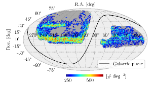
(a) DESI DR1 LRG.

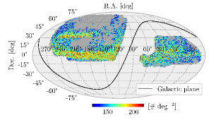
(b) DESI DR1 QSO.

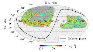
(c) LRG corrected by the completeness.

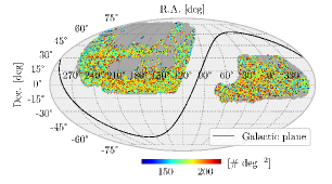
(d) QSO corrected by the completeness.

Figure 1: Angular density distribution for the DESI DR1 LRG/QSO on the left/right corrected by the completeness of the observation (some regions of the sky have yet to be fully observed) on the bottom and not on the top. The comparison between top and bottom panel shows from which region the statistical information comes from. Although both appear almost isotropic, one must correct for the anisotropy due to the dependence of the target selection on the image quality. The dark gray region represents the expected final DESI footprint.

The target selection of the LRGs and QSOs are based on the DESI Legacy Imaging Survey [56] that contains four different photometric regions with different image qualities, see Fig. 1 of [57] for instance. These photometric regions are called:

• North is the northern part of the footprint in the North Galactic cap (NGC) ($\mathrm{Dec.}>32.375~{}\rm{deg}$) corresponding to the part of the sky covered by BASS [58], and MzLS [59].

• DES is the region covered by the Dark Energy Survey [60] and is significantly deeper than the rest of the footprint.

• South (NGC) is the rest of the footprint in NGC, which was also collected by DECam [61] but is less deep than DES.

• South (SGC) is similar to South (NGC) but in the South galactic cap (SGC). We split South (NGC) and South (SGC) although they have similar photometry because the two regions are spatially disjointed, and thus are never used in the same time when we compute the power spectrum either on the full NGC or SGC.

The target selection for the LRGs is the same across each region [53]; however, to adapt to each region specificities, the target selection for the QSOs is adapted for each region [54]. The discrepancy in either the target selection or imaging quality leads to different mean densities in these different photometric regions, as given in Table 1, and slightly different redshift distributions as displayed in Figure 2. In particular, DES has more high-$z$ quasars than the others because the imaging is deeper, and DES and North have less low-$z$ quasars than the South since the PSF is better resolved, such that low-$z$ quasars are preferentially detected with a non-PSF morphology and therefore do not pass the cut on PSF-like objects imposed by the QSO target selection, see Fig.11 in [54]. Therefore, in the following, these regions are always treated separately and mutually renormalised before computing the power spectrum over the entire NGC or SGC, see Section 3.2.4.

Table 1: Mean density of the LRG and QSO samples (corrected by the completeness of the observation) in each photometric region.

	LRG $[\rm{deg}^{-2}]$	QSO $[\rm{deg}^{-2}]$
North	$531.7$	$184.5$
South (NGC)	$535.3$	$186.6$
South (SGC)	$532.6$	$187.2$
Des	$519.5$	$191.7$

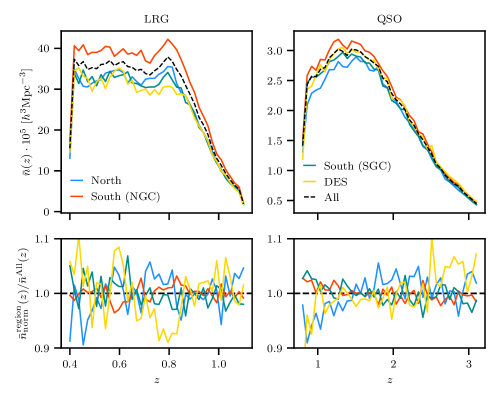
Figure 2: On the top, the redshift distributions for the LRGs (left) from 0.4 to 1.1 and QSOs (right) from 0.8 to 3.1 not corrected by the completeness of the observation, split according to the four distinct photometric regions: North in blue, South (NGC) in red, South (SGC) in green and DES in gold. The black dashed line is for the four regions combined. The difference in amplitudes highlights the difference of completeness between the different footprints. There are more objects in South (NGC) because it is the area that is the most complete, see Figure 1. On the bottom, the ratio between the redshift distributions of the different photometric regions and the ones from the four regions combined. At the bottom panel, redshift distributions are normalized to have the same amplitude than the ones from the four regions combined. The redshift distributions are remarkably similar for the LRGs; some differences in the North are visible for the QSOs.

The construction of the catalogues for the data and the randoms are described in [62], and [63, 64, 65] describe the spectroscopic reduction pipeline, as well as, the redshift estimation from the spectra. We only discuss, in the following, the correction of the imaging dependence of the target selection, see Section 5.3.2. During this analysis, we only use ten files of randoms instead of 18 as in the fiducial BAO [31] and RSD [33] analysis, and after comparison, we denote no impact on the scales of the power spectrum that we use.

Note that at this stage of the DESI DR1 analysis and with the standard treatment, the large-scale modes of the Emission Line Galaxy (ELG) sample [66] are not yet fully reliable despite a significant effort and development of new tools [67] and are therefore not used here. See, in particular, the large-scale modes of the ELGs power spectrum displayed in Section A.2 that exhibit an unexpected excess of power about one magnitude. One could only analyse smaller scales ($k>0.008~{}h\text{Mpc}^{-1}$) where the power spectrum seems more reasonable, but due to the low linear bias of this tracer, no interesting constraints can be extracted at present.

3.1.2 Correct for observational systematics

As described in [62], one needs to correct the data for several observational effects by weighting them with

$$w_{\rm tot}=w_{\rm comp}\times w_{\rm sys}\times w_{\rm zfail}.$$ (3.1)

The different contributions in Eq. 3.1 are for

• Completeness ($w_{\rm comp}$): The complex geometry of the survey is taken into account via the randoms, uniform distribution of objects without any clustering which occupies the same volume as the data, and does not represent any difficulties. On the other hand, targets that are unobserved because there are no free fibers to observe them lead to a biased estimation of the power spectrum. The randoms cannot take these missing targets into account since the survey observes the geometrical regions associated with these missing targets. This impacts both large and small scales. The large scales can be easily corrected by the completeness weights $w_{\mathrm{comp}}$ that simply overweight the observed objects to match the number of total targets in the patrol radius of a fiber.

• Imaging systematics ($w_{\rm sys}$): Imaging systematics can be defined as the dependence of the target selection on the properties of the used photometric survey and create, unfortunately, an excess of correlation at large scales (see Section A.2). Since the imaging systematics are the major bias in our analysis, the mitigation of this contribution is carefully validated in Section 5.3.2.

• Spectroscopy efficiency ($w_{\rm zfail}$): Classification and redshift determination depend on the quality of the observation. Poor weather, noise in the CDDs, or dust in the sky can indeed impact the spectra collected. This effect is corrected but has a minor impact, as reported in [68, 69]. Note that any residual redshift determination errors are naturally be taken into account in our theoretical model, given in Eq. 2.4, by the parameter $\Sigma_{s}$ representing the typical damping velocity dispersion.

The completeness and redshift failures weights are the same as the ones summarized in [70], while the imaging systematic weights are fully re-determined for this analysis, see Section 5.1.

Since the randoms should reproduce the same redshift distribution as the data, we randomly draw the redshifts and associated weights from the data for the randoms, such that randoms have similar weights ($w_{\mathrm{tot},r}$). This procedure is known as the shuffling method [71] and impacts the measurement as described in Section 4.4.

3.1.3 Blinding the data

To avoid any confirmation bias during our analysis, we have developed a blinding scheme that reproduces the scale-dependent bias in the power spectrum. This blinding is described and validated in [72]. Note that this is the first time the scale-dependent bias has been measured with a blinding strategy.

Similar to the blinding schemes applied to conceal the BAO and RSD signal [73], this blinding is applied at the catalog level. The one for PNG is a set of weights reproducing a value of $f_{\rm NL}^{\rm blind}\in[-15,15]$ randomly chosen, such that the amount of PNG measured from the blinded data, $f_{\rm NL}^{\rm obs}$, is

$$f_{\rm NL}^{\rm obs}=f_{\rm NL}^{\rm loc}+f_{\rm NL}^{\rm blind}.$$ (3.2)

These weights are multiplied by the completeness weights, preventing anyone from breaking the blinding since the large-scale modes of the power spectrum cannot be recovered without correcting for completeness.

As described in [72], the blinding is applied coherently across all the samples such that one can compare the large-scale modes of the power spectrum measured from sub-part of the sample, allowing us internal consistency validation, see Section 5.3.1. Although the blinding value $f_{\rm NL}^{\rm blind}$ is the same for the different tracers, the weights were generated with a value of $b_{\Phi}$ computed for $p=1.0$ in each situation so that the apparent blinding value for the QSO when analysing with $p=1.6$ should be larger in absolute value.

3.1.4 Linear bias evolution

Table 2: Value of the parameters $(a,b)$ used to describe the redshift evolution of the linear bias $b_{1}$ as given in Eq. 3.3. These values are estimated from the unblind DESI DR1 LRG and QSO samples.

	$a$	$b$
LRG	$0.209\pm 0.025$	$1.415\pm 0.076$
QSO	$0.237\pm 0.010$	$0.771\pm 0.070$

The evolution of the linear bias can modeled by

$$b_{1}(z)=a(1+z)^{2}+b,$$ (3.3)

where $a,b$ are given for LRGs and QSOs in Table 2. These two parameters are measured from the unblind DESI DR1 LRG and QSO samples. The measurement is detailed in Section A.1.

3.2 Measuring the power spectrum from a spectroscopic survey

3.2.1 Power spectrum estimator

In the following, the multipoles of the power spectrum are estimated through the so-called Yamamoto estimator [74]. The estimation of the average power spectrum $\hat{P}\left(\mathbf{k}_{\mu}\right)$, in a phase-space volume $V_{\mathbf{k}_{\mu}}$ corresponding to the binning used in $\mathbf{k}_{\mu}$ space for the measurement, is given by

$$\hat{P}_{\ell}\left(k_{\mu}\right)=\dfrac{2\ell+1}{AV_{k_{\mu}}}\int_{V_{k_{\mu}}}\differential\mathbf{k}\int\differential\mathbf{x}_{1}\int\differential\mathbf{x}_{2}\,e^{i\mathbf{k}\cdot\left(\mathbf{x}_{2}-\mathbf{x}_{1}\right)}\mathcal{F}\left(\mathbf{x}_{1}\right)\mathcal{F}\left(\mathbf{x}_{2}\right)\mathcal{L}_{\ell}\left(\hat{\mathbf{k}}\cdot\hat{\mathbf{x}}_{1}\right)\\ -\mathcal{N}_{\ell}~{},$$ (3.4)

where we use the first-point $\mathbf{x}_{1}$ as the line-of-sight instead of the midpoint line-of-sight to speed up the computation (see below), $F(\mathbf{x})$ is the FKP field [75] estimated from the data and the random catalogues

$$\mathcal{F}(\mathbf{x})=n_{g}(\mathbf{x})-\alpha n_{r}(\mathbf{x})\quad\text{ with }\quad\alpha=\dfrac{\int\differential\mathbf{x}\,n_{g}(\mathbf{x})}{\int\differential\mathbf{x}\,n_{r}(\mathbf{x})}~{},$$ (3.5)

where $n_{g}$ is the galaxy weighted density, $w_{g}=w_{\mathrm{FKP}}\times w_{\rm tot}$, and $n_{r}$ the randoms’ one, $w_{r}=w_{\mathrm{FKP}}\times w_{\mathrm{tot},r}$. The randoms are used to sample the survey geometry, more specifically the survey selection function $W(\mathbf{x})$, which is the ensemble average of the galaxy density:

$$W(\mathbf{x})\equiv\left\langle n_{g}(\mathbf{x})\right\rangle=\alpha\left\langle n_{r}(\mathbf{x})\right\rangle.$$ (3.6)

The FKP weights [75], $w_{\mathrm{FKP}}$, are weighting scheme that improve the power spectrum measurement by minimising the expected errors of $\hat{P}\left(\mathbf{k}_{\mu}\right)$:

$$w_{\mathrm{FKP}}(\mathbf{x},\mathbf{k})=\dfrac{1}{1+\bar{n}_{g}(\mathbf{x})P(\mathbf{k})}~{},$$ (3.7)

where $P(\mathbf{k})$ is fixed as about the maximal amplitude measured in the data around $k_{\rm eq}$ which are the scales of interest: $P(\mathbf{k})=P_{0}=3\times 10^{4}~{}\left(\mathrm{Mpc}/h\right)^{3}$ for the QSO and $5\times 10^{4}~{}\left(\mathrm{Mpc}/h\right)^{3}$ for the LRG. In what follows, FKP weights are computed independently in each of the four photometric regions using the redshift distributions displayed in Figure 2.

Additionally, the normalization factor used in Eq. 3.4 is given by

$$A=\int\differential\mathbf{x}\,\bar{n}_{g}(\mathbf{x})^{2},$$ (3.8)

and the shot noise contribution is removed with

$$\mathcal{N}_{\ell}=\dfrac{\delta_{\ell 0}}{A}\int\differential\mathbf{x}\,W(\mathbf{x})\left[w_{g}(\mathbf{x})+\alpha w_{r}(\mathbf{x})\right].$$ (3.9)

Finally, the choice of $\mathbf{x}_{1}$ as a line-of-sight coordinate reduces the computation time of Eq. 3.4, by splitting the double integral [74],

$$\hat{P}_{\ell}\left(k_{\mu}\right)=\dfrac{2\ell+1}{AV_{k_{\mu}}}\int_{V_{k\mu}}\differential\mathbf{k}\,F_{0}(\mathbf{k})F_{\ell}(-\mathbf{k})-\mathcal{N}_{\ell}~{},$$ (3.10)

where we have introduced

$$F_{\ell}(\mathbf{k})=\int\differential\mathbf{x}\,e^{i\mathbf{k}\cdot\mathbf{x}}\mathcal{F}(\mathbf{x})\mathcal{L}_{\ell}(\hat{\mathbf{k}}\cdot\hat{\mathbf{x}}).$$ (3.13)

Note that this choice of line-of-sight leads to the so-called wide-angle effects that is described in Section 4.1.

In the following, all power spectra are computed with pypower using the Triangular Shaped Cloud (TSC) sampling and interlacing at order $n=3$ to mitigate the aliasing. For both LRG and QSO samples, we use a physical box sizes of $16000~{}h^{-1}\mathrm{Mpc}$ with a grid cell size of $6~{}h^{-1}\mathrm{Mpc}$, leading to a Nyquist frequency of $k_{N}\sim 0.5~{}h\mathrm{Mpc}^{-1}$.

3.2.2 Optimal quadratic estimator for the scale-dependent bias

The FKP weights introduced above miss the redshift dependence of the PNG signal that we want to measure, such that introduce this dependence into the FKP weights provides a more optimal way to extract the scale-dependent bias signal in the power spectrum. This can be achieved by using optimised redshift weights that are inspired from the optimal quadratic estimator (OQE) for $f_{\rm NL}^{\rm loc}$ [77, 39]. In the following, we follow [39] who propose to weight each galaxy, which is more natural to compute the FKP field $\mathcal{F}$, instead of weighting pairs of galaxies as in [8].

The optimal estimator for extracting $f_{\mathrm{NL}}^{\mathrm{loc}}$ has the same form as Eq. 3.10 but with a different weighting scheme:

$$\hat{P}_{\ell}\left(k_{\mu}\right)=\dfrac{2\ell+1}{A_{\ell}V_{k_{\mu}}}\int_{V_{k\mu}}\differential\mathbf{k}\,\tilde{F}(\mathbf{k})F_{\ell}(-\mathbf{k})-\mathcal{N}_{\ell},$$ (3.14)

where

$$\left\{\begin{array}[]{ll}\tilde{F}(\mathbf{k})&=\displaystyle\int\differential\mathbf{x}\,e^{i\mathbf{k}\cdot\mathbf{x}}\tilde{w}\left(\mathbf{x}\right)\mathcal{F}(\mathbf{x})\\[3.0pt] F_{\ell}(\mathbf{k})&=\displaystyle\int\differential\mathbf{x}\,e^{i\mathbf{k}\cdot\mathbf{x}}w_{\ell}\left(\mathbf{x}\right)\mathcal{F}(\mathbf{x})\mathcal{L}_{\ell}(\hat{\mathbf{k}}\cdot\hat{\mathbf{x}})\end{array}\right.,$$ (3.15)

and the shot noise contribution is

$$\mathcal{N}_{\ell}=\dfrac{\delta_{\ell 0}}{A}\int\differential\mathbf{x}\,W(\mathbf{x})\left[w_{g}(\mathbf{x})+\alpha w_{r}(\mathbf{x})\right]\tilde{w}\left(\mathbf{x}\right)w_{\ell}\left(\mathbf{x}\right).$$ (3.16)

Similarly, the normalization factor in Eq. 3.8 becomes

$$A_{\ell}=\int\differential\mathbf{x}\,\bar{n}_{g}(\mathbf{x})^{2}\tilde{w}\left(\mathbf{x}\right)w_{\ell}\left(\mathbf{x}\right).$$ (3.17)

The optimal weights $\tilde{w}$, $w_{0}$ and $w_{2}$ for the quadratic estimator are

$$\left\{\begin{array}[]{ll}\tilde{w}(z)&=\left[b(z)-p\right]\\[3.0pt] w_{0}(z)&=D(z)\left[b(z)+f(z)/3\right]\\[3.0pt] w_{2}(z)&=2/3D(z)f(z)\end{array}\right.,$$ (3.18)

where $p$ is the parametrization used for $b_{\Phi}$ in Eq. 2.6, $f$ is the growth rate and $D$ is the growth factor.

These weights used in this analysis are displayed in Figure 3 for the LRG and QSO samples. For the LRGs (left panel), the shapes of $\tilde{w}$, $w_{0}$ and $w_{2}$ are very similar to $w_{\rm FKP}$ such that we do not expect substantial improvement by using these optimal weights compared to the traditional FKP ones. The FKP weight shape, increasing a lot around $z\sim 1$, comes from the decrease of the density $n(z)$ of this sample in this region.

For the QSOs (right panel), the optimal weights in Eq. 3.18 overweight the objects at high redshift, naturally increasing the effective redshift of the sample. The first effect is to increase the value of $b_{1}$ and $b_{\Phi}$ in our weighted sample such that the precision on $f_{\rm NL}^{\rm loc}$ is improved. Due to this effective redshift modification, it is hard to quantify precisely how these weights improve the measurement compared to the standard FKP weights.

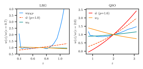
Figure 3: Optimal weighting scheme used to measure $f_{\rm NL}^{\rm loc}$ for LRG sample (left) and QSO sample (right) as a function of redshift. The usual FKP weights are displayed in blue. For the quasars, the most important weight is $\tilde{w}$, which follows the redshift evolution of the linear bias. For comparison, we normalize the weight to one at $z=0.7$ for the LRGs and $z=2.0$ for the QSOs.

Practically speaking, computing the power spectrum with the OQE weights is just the cross-power spectrum between one FKP field weighted by $\tilde{w}$ and another one weighted by $w_{\ell}$. Therefore, the computation of the power spectrum causes no problem.

Since the bias vanishes in the hexadecapole ($\ell=4$), no specific weights are needed for this multipole. Due to a lack of statistical significance, we do not include the hexadecapole in our analysis. The gain by using the quadrupole ($\ell=2$) in addition to the monopole ($\ell=0$) is shown in Section A.4.

3.2.3 Effective redshift

During the parameter estimation step, one needs to evaluate the model Eq. 2.4 at the effective redshift of the data. We are following the definition used in [39] that is correct up to first order in the Taylor expansion:

$$z_{\mathrm{eff}}=\frac{\int\differential z\,n(z)^{2}w_{a}(z)w_{b}(z)z}{\int\differential z\,n(z)^{2}w_{a}(z)w_{b}(z)},$$ (3.19)

where $w_{a},w_{b}$ are the weights of two fields that are cross-correlated.

Table 3 gives the effective redshift under the different sets of weights used in the following. The redshift distribution of the DR1 LRGs and QSOs are displayed in Figure 2. For comparison, we also give the effective redshift without any weighting scheme and the effective redshift for the quasars when using $p=1.0$. Using OQE weights significantly increases the effective redshift for the quasar, while it is less pronounced for the LRG since the $n(z)$ is mostly flat. Using $p=1.6$ reduces the response of the scale-dependent bias to the presence of PNG such that the OQE weights increase the weight for the higher redshift part of the sample, where the signal is the most important.

Note that the use of OQE weights requires to evaluate the linear power spectrum at two different effective redshifts, one for the monopole and one for the quadrupole. In the following, when we use the OQE weights with $\ell=0,2$, we assume that $\Sigma_{s}$ does not depend on the redshift while we fit $b_{1}$ by considering the evolution given in Eq. 3.3.

Table 3: Effective redshift for the DESI DR1 LRG and QSO samples computed with the completeness and spectroscopic efficiency weights. For comparison, the mean redshift of the samples is displayed in the first line, and the unweighted effective redshift in the second one. Due to the shape of the redshift distribution, using OQE weights significantly increases the effective redshift for the quasars.

	LRG	QSO
	0.4 < z < 1.1	0.8 < z < 3.1
$\bar{z}$	0.741	1.768
$z_{\mathrm{eff}}$	0.665	1.573
$z_{\mathrm{eff}}$ (FKP)	0.733	1.651
$z_{\mathrm{eff}}$ (OQE $\ell=0$, $p=1.0$)	0.754	1.926
$z_{\mathrm{eff}}$ (OQE $\ell=2$, $p=1.0$)	0.751	1.813
$z_{\mathrm{eff}}$ (OQE $\ell=0$, $p=1.6$)	-	2.082
$z_{\mathrm{eff}}$ (OQE $\ell=2$, $p=1.6$)	-	1.989

3.2.4 Normalization across the different photometric regions

As shown in Table 1 and in Figure 2, the LRG [53] and QSO [54] samples have different redshift distributions and angular densities in different photometric regions of the Legacy Imaging Surveys used for the target selection: North, South and DES. These differences may be due to slightly different target selection cuts or to different photometric properties of a specific region. For instance, the DES region is about one magnitude deeper than South [56].

Although one can compute the power spectrum independently on each of these photometric regions, one wants to compute the power spectrum simultaneously on the different regions to avoid losing any modes across the different regions and reduce the statistical uncertainty of our measurement. In the following, the power spectrum is computed on all the NGC and on all the SGC such that we need to normalize the North to the South (NGC) and DES to the South (SGC).

Here, the normalization of the randoms means that $\alpha$ in Eq. 3.5 is set to match the corresponding data separately in each region. Thus, the randoms weights in the South (NGC) are multiplied by the normalization factor:

$$f_{\textrm{norm}}=\dfrac{\sum_{i\in\textrm{North}}w_{r,i}}{\sum_{i\in\textrm{North}}w_{d,i}}\times\dfrac{\sum_{i\in\textrm{South (NGC)}}w_{d,i}}{\sum_{i\in\textrm{South (NGC)}}w_{r,i}},$$ (3.20)

and similarly for the weights in the South (SGC) (South (NGC), North $\rightarrow$ South (SGC), DES).

This normalization is crucial to measure the power spectrum’s large-scale modes without bias. The impact of the normalization of DES to South (SGC) is shown in Section A.3.

3.3 Estimating the covariance matrix

3.3.1 EZmocks

In the following, the covariance matrix is estimated as the covariance between the measurements done in a large set of realistic simulations (mocks) that emulate the observations as faithfully as possible.

As in eBOSS [79], we choose the approximate method known as EZmocks [80] to generate our realistic simulations. This method generates a galaxy field with position and velocity that follows an input power spectrum at an effective redshift, thanks to the Zel’dovich approximation [81]. This approximation is enough in our situation since our analysis is focused on large scales where the linear theory holds such that the EZmocks predict the desired covariance matrix [82].

We use the EZmocks generated for DESI that are similar to what is described in [79]. For a full description of these simulations, we refer the reader to [83]. In particular, we use 2000 boxes of $6~{}\mathrm{Gpc}~{}h^{-1}$ side, 1000 for the NGC and 1000 for the SGC, so that we do not need duplications to cover the full volume of DESI. Boxes for the LRGs (resp. QSOs) are generated at $z=0.8$ (resp. $z=1.4$) using the fiducial DESI cosmology. Despite the large size of these boxes, quasars are too dispersed in redshift such that they can be emulated only up to $z_{\rm max}=3.1$ without repeating the box. It explains why we stop our analysis at this maximum redshift for the quasars, although DESI has observed quasars at higher redshifts, $\sim$32,500 with $3.1<z<3.5$.

In Section 5.7 of [32] (see also Section 10.2 of [70]), the covariance matrix from the EZmocks is rescaled to match the analytical prediction from RascalC [84]. Here, however, we do not rescale our covariance matrix. The difference arises because the EZmocks in [32] incorporate a method to emulate the fiber assignment of DESI known as the FFA [85] (see Section 11.2 of [70]), which results in an underestimation of the variance. In our case, we neglect the impact of the fiber assignment and we verified that our EZmocks do not under-estimate the covariance. Further investigations could be required for the upcoming data release.

3.3.2 Generate realistic simulations

First, the cubic EZmocks are remapped according to [86] to increase the sky coverage of these simulations, and all the coordinates are transformed into sky coordinates ($\mathrm{R.A.},\mathrm{Dec.},z$) after the remapped box is moved along an axis. Then, we add the redshift space distortion effect along the line-of-sight by translating the real space position to redshift space [42].

Next, we match these simulations to the DESI survey. We imprint the redshift distribution (Figure 2) and the mean density (Table 1) independently in each of the photometric regions. At that time, we did not differentiate between South (NGC) and South (SGC), and we used the redshift distribution and density from South (NGC+SGC) for the two regions. This will be improved with the upcoming DESI data release and is neglected in the following.

Since the large-scale modes of the power spectrum are insensitive to the fiber assignment, we can only apply the global completeness by downsampling the data and the randoms via an HEALPix map [87, 88] at $N_{\rm side}=256$ representing the fraction of the pixel that was observed in DESI DR1. We finally remove objects located in bad imaging regions as in [62]. In particular, we use the LRG mask developed in [53] for the LRGs and the imaging maskbits 1, 7, 8, 11, 12 and 13 for the QSOs. This is not exactly what it is done in [70] that, in addition, also removes pixels where the imaging properties of the photometric survey are too extreme and regions with bad hardware. This represents a small fraction of the sky that is negligible for our covariance matrix estimation compared to the expected statistical errors.

We also generate, from the same boxes, mocks that describe the expected final DESI sample after the five years of observation referred in the following as Y5. We use the exact sky coverage to match the expected observations and assume full completeness and the same redshift distribution and density for each photometric region as the DR1 sample. These Y5 mocks will be used to have an accurate forecast for the expected final DESI sample and validate our theoretical description, see Section 4.2.

3.3.3 Computing the covariance matrix

Once each mock realization is matched to DESI DR1, the power spectrum with different sets of weights (FKP or OQE) is computed precisely in the same way as the one calculated from the data, as explained in Section 3.2. Figure 4 shows the power spectrum of the mean of 1000 EZmocks for LRGs (left) and QSOs (right) as well as the power spectrum from the blinded data catalog. The coloured shaded regions represent the $\pm 1\sigma$ deviation estimated from 1000 realizations. Although the EZmocks were not generated at the correct effective redshift of the data (see Table 3), they remain usable to estimate the covariance matrix because they match the amplitude of the power spectrum from the data, and our analysis is limited to scales that are almost linear.

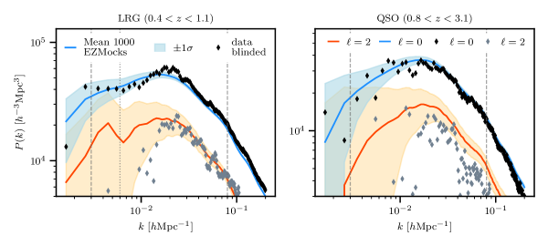
Figure 4: Comparison between the multipoles (NGC+SGC) from the mean of 1000 EZmocks (solid lines) and the blinded data (diamond points) for the LRGs (left) and the QSOs (right). The coloured dashed regions are the $\pm 1\sigma$ regions from the EZmocks. Note that although the large scales are blinded for the data, there is a good agreement between the mean from the EZmocks and the data. The discrepancy at large scales on the quadrupole is from the radial integral constraints and is detailed in Section 4.4.

Finally, the covariance $C_{ij}$ is simply the covariance between these 1000 measured power spectra. As proposed in [89], we re-scale by multiplying the inverse of the covariance by the Hartlap factor to deal with the skewed nature of the inverse Wishart distribution as

$$C_{ij}^{-1}\longleftarrow\dfrac{N_{m}-n-2}{N_{m}-1}C_{ij}^{-1},$$ (3.21)

where $N_{m}$ is the number of mocks, and $n$ is the number of data points. In addition, we also add the extra correction provided in [90] to correct for the propagation of errors in the covariance matrix to the errors on estimated parameters, re-scaling Eq. 3.21 by dividing it by the Percival factor

$$C_{ij}^{-1}\longleftarrow\left(\dfrac{1+B(n-n_{p})}{1+A+B(n_{p}+1)}\right)^{-1}C_{ij}^{-1},$$ (3.22)

with $A=2\left[\left(N_{m}-n-1\right)\left(N_{m}-n-4\right)\right]^{-1}$, $B=\left(N_{m}-n-2\right)\left[\left(N_{m}-n-1\right)\left(N_{m}-n-4\right)\right]^{-1}$ and $n_{p}$ the number of estimated parameters. Typically, in the following, $N_{m}=1000$, $n=116$, and $n_{p}=4$ such that the Hartlap factor evaluates to $\sim 0.88$ and the Percival factor to $\sim 1.12$.

Note that in practice, all the inference is performed using the desilike framework. The posterior profiling is performed through the iminuit [91] minimiser and all the Monte Carlo Markov chains (MCMC) use the emcee [92] sampler.

4 Modeling of geometrical effects

The large-scale modes of the observed power spectrum are impacted by the geometry of the survey. In this section, we present how to modify our model in order to account for the geometry as well as correct for the integral constraints.

4.1 Window function and wide-angle effect

Due to stars, Milky Way dust, or incompleteness of the observations, some parts of the footprint are masked or unobserved such that we do not exactly observe the full density field, but only a fraction of it. This is described by the survey selection function $W(\mathbf{x})$, see Eq. 3.6. Hence, the expected value of the power spectrum estimator in Eq. 3.10 reads as

$$\left\langle\hat{P}_{\ell}(k)\right\rangle=\dfrac{(2\ell+1)}{A}\int\dfrac{\differential\Omega_{k}}{4\pi}\int\differential\mathbf{s_{1}}\int\differential\mathbf{s_{2}}\,e^{i\mathbf{k}\left(\mathbf{s_{2}}-\mathbf{s_{1}}\right)}\xi(\mathbf{s_{1}},\mathbf{s_{2}})W\left(\mathbf{s_{1}}\right)W\left(\mathbf{s_{2}}\right)\mathcal{L}_{\ell}\left(\hat{\mathbf{k}}\cdot\hat{\mathbf{s_{1}}}\right)$$ (4.1)

Following [93], the correlation function can be expanded into Legendre multipoles and under the local plane-parallel approximation limit ($s\ll s_{1},s_{2}$ with $\mathbf{s}=\mathbf{s_{1}}-\mathbf{s_{2}}$), Eq. 4.1 becomes

$$\left\langle\hat{P}_{\ell}(k)\right\rangle= \dfrac{(2\ell+1)}{A}\sum_{p}\int\dfrac{\differential\Omega_{k}}{4\pi}\int\differential\mathbf{x}\int\differential\mathbf{s}\,e^{-i\mathbf{k}\cdot\mathbf{s}}W(\mathbf{x})W(\mathbf{x}-\mathbf{s})\xi_{p}(s)\mathcal{L}_{p}(\hat{\mathbf{x}}\cdot\hat{\mathbf{s}})\mathcal{L}_{\ell}(\hat{\mathbf{k}}\cdot\hat{\mathbf{x}})$$ (4.2)

$$=4\pi(-i)^{\ell}(2\ell+1)\sum_{\ell_{1},\ell_{2}}\left(\begin{array}[]{ccc}\ell_{1}&\ell_{2}&\ell\\ 0&0&0\end{array}\right)^{2}\int\differential s\,s^{2}j_{\ell}(ks)\xi_{\ell_{1}}(s)\mathcal{W}_{\ell_{2}}(s)$$

where we have introduced the real space window matrix

$$\mathcal{W}_{\ell}(s)\equiv\dfrac{(2\ell+1)}{4\pi\times A}\int\differential\Omega_{s}\int\differential\mathbf{x}\,W(\mathbf{x})W(\mathbf{x}-\mathbf{s})\mathcal{L}_{\ell}(\hat{\mathbf{x}}\cdot\hat{\mathbf{s}}).$$ (4.3)

To speed up the computation of the Eq. 3.4, we have chosen the first galaxy as the line-of-sight [74]. This is a good choice under the local plane-parallel approximation. However, this choice creates the so-called wide-angle effect when this approximation does not hold [94]. One can take into account this wide-angle effect by expanding the theoretical correlation function as

$$\xi\left(\mathbf{x}_{1},\mathbf{x}_{2}\right)=\sum_{p,n}\left(\frac{s}{d}\right)^{n}\xi_{p}^{(n)}(s)\mathcal{L}_{p}(\hat{\mathbf{d}}\cdot\hat{\mathbf{s}}),$$ (4.4)

where $\mathbf{s}=\mathbf{x_{2}}-\mathbf{x_{1}}$ is the pair separation and $\mathbf{d}$ the line-of-sight.

As described in [93], the wide-angle effect can be easily handled with the above window matrix formalism by introducing the $(s/d)^{n}$ expansion in Eq. 4.2, and one need to compute new window matrices

$$\mathcal{W}_{\ell}^{(n)}(s)=\dfrac{2\ell+1}{4\pi\times A}\int\differential\Omega_{s}\int\differential\mathbf{x}\,x^{-n}W(\mathbf{x})W(\mathbf{x}-\mathbf{s})\mathcal{L}_{\ell}(\hat{\mathbf{x}}\cdot\hat{\mathbf{s}}).$$ (4.5)

In the following, we only consider the first order of the effect ($n=1$) such that

$$\left\{\begin{array}[]{ll}\xi_{1}^{(1)}(s)&=-\dfrac{3}{5}\xi_{2}^{(0)}(s)\\[3.0pt] \xi_{3}^{(1)}(s)&=\dfrac{3}{5}\xi_{2}^{(0)}(s)-\dfrac{10}{9}\xi_{4}^{(0)}(s)\end{array}\right.,$$ (4.6)

and the multipoles of the correlation function $\xi_{\ell}^{(0)}$ are computed from Eq. 2.4 and Eq. 2.5 using

$$\xi_{\ell}^{(0)}(r)=\frac{i^{\ell}}{2\pi^{2}}\int\differential k\,k^{2}j_{\ell}(kr)P_{\ell}(k).$$ (4.7)

Hence, the convolved power spectrum is evaluated on a finite size wavelength vector $k_{i}$ through a single matrix multiplication

$$\left(P_{\ell}^{\rm obs}\right)_{i}=\left(\mathcal{W}_{\ell\ell^{\prime}}\right)_{ij}\left(P_{\ell^{\prime}}\right)_{j},$$ (4.8)

where the summation run over $\ell^{\prime}$ and $j$ the indices on which the unconvolved power is evaluated.

The real space window matrix for the DESI DR1 LRG and QSO sample is displayed in Figure 5. One can note that, as indicated by [95], the real space window matrix $\mathcal{W}_{0}(s)$ is not normalised to 1 when $s\rightarrow 0$. The normalization factor is the same as the one used in Yamamoto’s estimator Eq. 3.10 and does not introduce a bias during the parameter estimation.

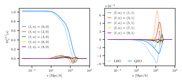
Figure 5: Real space window matrix for the DESI DR1 LRG (dashed lines) and QSO (solid lines) sample. The window matrices without the wide-angle effect ($n=0$) are displayed on the left, while the first order ($n=1$) contribution are displayed on the right.

The multipoles of the theoretical convolved power spectrum accounting for the geometry of the DESI DR1 LRG or QSO sample are shown in Figure 6. The impact on large scales of the window matrix cannot be neglected when measuring the large-scale modes of the power spectrum. Additionally, the impact of considering the wide-angle effect is displayed in left panel. As expected, no strong effects are visible for the QSOs, since the quasars are sufficiently far away from us for the local plane-parallel approximation to hold. However, the effect is larger for the LRG but is still very small such that we do not account for high-order contribution ($n\geq 2$) of the wide-angle effect [96].

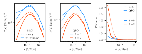
Figure 6: Multipoles of the convolved (resp. unconvolved) power spectrum are displayed in solid (resp. dashed) lines for the DESI DR1 LRG (left panel) and QSO (middle panel) sample. Right panel shows the ratio between the convolved power spectrum accounting for the first order wide-angle effect and not accounting for it. As expected the wide-angle effect is bigger for the LRG that are closer to us.

In practice, the window matrix is computed from the random catalog that fully described the geometry of the data, using the implementation available in pypower. Then the convolution of the model with the window function is done in desilike. As in [97], we only use the multipoles up to $\ell=4$ in Eq. 4.2 such that we only consider the window matrix up to $\ell=8$.

4.2 Validation with EZmocks

4.2.1 Analysis setup

One can use the mean of the power spectrum over the 1000 EZmocks as a null test, to validate the theoretical prediction given in Eq. 4.8 and forecast with great accuracy the statistical errors expected for this analysis. During the MCMC and the profiling, we fit either $(f_{\rm NL}^{\rm loc},b_{1},s_{n,0},\Sigma_{s})$ assuming Eq. 2.6 or $(b_{\Phi}f_{\rm NL}^{\rm loc},b_{1},s_{n,0},\Sigma_{s})$ together.

First, as explained in Section 3.3.1, the EZmocks were not generated at the correct effective redshift with the correct bias. Fortunately, the amplitudes of the power spectrum of these EZmocks match quite well the one from the data, see Figure 4, such that they can be used without renormalization to build the covariance matrix. However, to use them as a null test, we need to match the amplitude to recover the expected bias at a specific effective redshift by renormalising the monopole and the quadrupole. This does not pose any problems, as we mainly use linear scales of the power spectrum. This can be achieved by measuring the actual bias $b$ from the mocks at $z_{\rm eff}$ and then replacing the multipoles by

$$\left\{\begin{array}[]{ll}P_{0}(k)&\longrightarrow\dfrac{b_{n}^{2}}{b^{2}}\dfrac{1+2/3\beta_{n}+1/5\beta_{n}^{2}}{1+2/3\beta+1/5\beta^{2}}\times P_{0}(k)\\ P_{2}(k)&\longrightarrow\dfrac{b_{n}^{2}}{b^{2}}\dfrac{4/3\beta_{n}+4/7\beta_{n}^{2}}{4/3\beta+4/7\beta^{2}}\times P_{2}(k)\end{array}\right.,$$

where $b_{n}$ is the desired bias and $\beta_{n}=f(z_{\rm eff})/b_{n}$ (similarly for $\beta$).

Next, we quantify the dependence of the statistical error as a function of the range that it is used during the fit. This dependence is shown in Figure 7 for the different tracers and the different weighting scheme. This range is limited by two factors:

• $k_{\rm min}$: At large scales, the measurement is impacted either by a mismodeling of the geometrical effects or by a imperfect correction of the imaging systematics (see Section 5). Due to the statistics, the very large-scales are not the most important ones as shown in the left panel of Figure 7, and we decide to use a conservative cut for our fiducial pipeline, avoiding any bias in our measurement: $k_{\rm min}=0.003~{}h\textrm{Mpc}^{-1}$. Note that the geometrical effects are still handled up to $k_{\rm min}=0.001~{}h\textrm{Mpc}^{-1}$, the limiting factor here is the efficiency of the imaging systematic mitigation.

• $k_{\rm max}$: At small scales, the simple description that we used, see Eq. 2.4, cannot deal with the non-linearity. As shown in the right panel of Figure 7, there is not much to gain by increasing $k_{\rm max}$ to constrain $f_{\rm NL}^{\rm loc}$. However, we still need some small-scale information to obtain a small uncertainty on $b_{1}$. Consequently, we choose to include the scales where the modes are mostly linear: $k_{\rm max}=0.08~{}h\textrm{Mpc}^{-1}$.

Hence, unless mentioned, all the fits in the following use

$$\left\{\begin{array}[]{ll}\ell_{0}:0.003<k<0.08\text{ with }\Delta k=0.001\quad h\mathrm{Mpc}^{-1}\\ \ell_{2}:0.003<k<0.08\text{ with }\Delta k=0.002\quad h\mathrm{Mpc}^{-1}\end{array}\right..$$

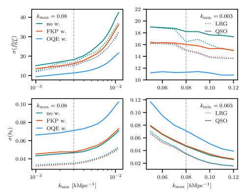
Figure 7: Dependence of the errors on $f_{\rm NL}^{\rm loc}$ (top) and $b_{1}$ (bottom) as a function of either $k_{\rm min}$ (left) or $k_{\rm max}$ (right) for the LRGs and the QSOs and for the different weighting schemes. The fiducial values, $k_{\rm min}=0.003~{}h\textrm{Mpc}^{-1}$ and $k_{\rm max}=0.08~{}h\textrm{Mpc}^{-1}$, are denoted with dashed vertical lines. Note that the errors here are the standard deviation from MCMC chains, however the distribution is not symmetric for $f_{\rm NL}^{\rm loc}$, see Figure 8. Therefore, the errors displayed here do not perfectly match those quoted in Table 4 that are the $1\sigma$ credible interval.

4.2.2 DR1 validation and Y5 forescast

Using the EZmocks as a null test, we can test our model with the fiducial scale range. The posteriors for the different tracers and weighting schemes are displayed in Figure 8 and the best fit values in Table 4. The second row in Figure 8 gives the posterior when considering $b_{\Phi}f_{\rm NL}^{\rm loc}$ as a single parameter without assuming any value for $b_{\Phi}$ and gives the overall sensitivity of the two tracers for the detection of the presence of primordial non-Gaussianity. For each configuration, we also give the measurement performed with mocks describing the DESI Y5 data.

In all the configurations, we recover $f_{\rm NL}^{\rm loc}=0$ well within $1\sigma$ validating the description of the geometrical effects described in Section 4.1. The difference between the value of the linear bias $b_{1}$ and the different weighting configurations is from the difference of effective redshift $z_{\rm eff}$, see Table 3. Although, there is a small discrepancy for the LRG DR1 EZmocks, it seems this is only a statistical fluctuation since it disappears when considering the Y5 footprint of the same realization. The systematic error contribution is discussed in Section 6.3. In addition, for the QSO case, one can notice a discrepancy between the value fitted with FKP and OQE weights; it will be discussed in Section 4.3.

As illustrated in Figure 8(b), the use of OQE weights helps to increase the value of $b_{1}$ since we are fitting the data with a higher effective redshift, see Table 3, which improves the constraint on $f_{\rm NL}^{\rm loc}$.

The constraints on $b_{\Phi}f_{\rm NL}^{\rm loc}$, given in Table 4, are better with the FKP weights compared to the OQE weights. This is not surprising, as the effective redshift, and due to the redshift evolution of $b_{1}$, the value of $b_{\Phi}$, is higher when using the OQE weights. This same reasoning explains why the errors on $f_{\rm NL}^{\rm loc}$ are smaller with OQE weights compared to FKP weights. Note that, without assuming any value for $b_{\Phi}$, we cannot obtain a competitive constraint with respect to Planck18 [7].

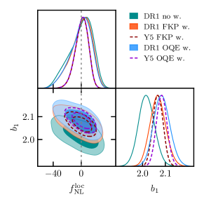
(a) LRG with $b_{\Phi}(b_{1})=2\delta_{c}(b_{1}-1)$.

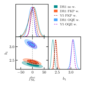
(b) QSO with $b_{\Phi}(b_{1})=2\delta_{c}(b_{1}-1.6)$.

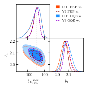
(c) LRG with $b_{\Phi}f_{\rm NL}^{\rm loc}$ as a free parameter.

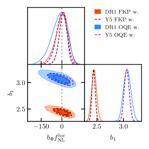
(d) QSO with $b_{\Phi}f_{\rm NL}^{\rm loc}$ as a free parameter.

Figure 8: Posteriors in the $(f_{\rm NL}^{\rm loc},b_{1})$ plane with $b_{\Phi}(b_{1})$ derived via Eq. 2.6 in (a) / (b) and in the $(b_{\Phi}f_{\rm NL}^{\rm loc},b_{1})$ plane in (c) / (d). The parameters $s_{n,0},\Sigma_{s}$ are free during the MCMC but are not shown for visibility. We fit the mean the 1000 realizations and use them to derive the covariance matrix. Filled contours are for the DR1 mocks while the dark dashed contours are for the Y5 mocks. Red colours are for the FKP weights, while the blue ones are for the OQE weights. For comparison, the case without any weighting is also included for the DR1 posteriors in green. The corresponding maximum-a-posteriori (MAP) values are displayed in Table 4.

Table 4: Results of the fit using the mean of the power spectrum over 1000 realizations with the corresponding covariance matrix for the LRGs and QSOs and the different weighting scheme. Central values are the best fit values from the minuit minimization while the errors are the $1\sigma$ credible interval from the chains that are displayed in Figure 8. The second part of the Table gives the best fits using $b_{\Phi}f_{\rm NL}^{\rm loc}$ as single parameter avoiding any assumption on the value of $b_{\Phi}$. The systematic error contribution is discussed in Section 6.3.

		$f_{\mathrm{NL}}^{\mathrm{loc}}$	$b_{1}$	$s_{n,0}$	$\Sigma_{s}$
LRG	DR1	$6_{-11}^{+21.}$	$2.010_{-0.036}^{+0.033}$	$0.048_{-0.065}^{+0.068}$	$4.45_{-0.44}^{+0.49}$
	DR1 (FKP)	$5_{-11}^{+18}$	$2.061_{-0.037}^{+0.032}$	$0.042_{-0.061}^{+0.064}$	$4.35_{-0.37}^{+0.52}$
	DR1 (OQE)	$5_{-11}^{+18}$	$2.077_{-0.035}^{+0.035}$	$0.040_{-0.058}^{+0.069}$	$4.32_{-0.42}^{+0.49}$
	Y5 (FKP)	$2.0_{-8.4}^{+10.7}$	$2.068_{-0.023}^{+0.022}$	$0.031_{-0.045}^{+0.042}$	$4.56_{-0.28}^{+0.31}$
	Y5 (OQE)	$2.2_{-7.6}^{+10.2}$	$2.083_{-0.023}^{+0.023}$	$0.029_{-0.044}^{+0.044}$	$4.52_{-0.28}^{+0.33}$
QSO	DR1	$3_{-16}^{+20}$	$2.339_{-0.051}^{+0.042}$	$-0.076_{-0.048}^{+0.057}$	$3.15_{-0.58}^{+1.19}$
	DR1 (FKP)	$3_{-13}^{+18}$	$2.442_{-0.045}^{+0.051}$	$-0.010_{-0.051}^{+0.056}$	$2.69_{-0.81}^{+1.22}$
	DR1 (OQE)	$-3_{-10}^{+13}$	$3.085_{-0.080}^{+0.064}$	$-0.045_{-0.074}^{+0.075}$	$0_{-0.93}^{+0.25}$
	Y5 (FKP)	$3.4_{-9.6}^{+9.9}$	$2.437_{-0.033}^{+0.030}$	$-0.292_{-0.037}^{+0.035}$	$3.43_{-0.39}^{+0.59}$
	Y5 (OQE)	$-2.4_{-7.8}^{+7.8}$	$3.086_{-0.049}^{+0.045}$	$-0.080_{-0.050}^{+0.053}$	$0_{-0.67}^{+0.19}$
		$b_{\Phi}f_{\mathrm{NL}}^{\mathrm{loc}}$	$b_{1}$	$s_{n,0}$	$\Sigma_{s}$
LRG	DR1 (FKP)	${21}_{-38}^{+68}$	${2.061}_{-0.035}^{+0.034}$	${0.041}_{-0.060}^{+0.066}$	${4.35}_{-0.43}^{+0.46}$
	DR1 (OQE)	${19}_{-41}^{+65}$	${2.077}_{-0.035}^{+0.036}$	${0.039}_{-0.065}^{+0.065}$	${4.32}_{-0.37}^{+0.54}$
	Y5 (FKP)	${9}_{-26}^{+37}$	${2.066}_{-0.021}^{+0.023}$	${0.034}_{-0.041}^{+0.047}$	${4.55}_{-0.27}^{+0.32}$
	Y5 (OQE)	${9}_{-24}^{+42}$	${2.082}_{-0.024}^{+0.023}$	${0.032}_{-0.044}^{+0.046}$	${4.50}_{-0.28}^{+0.33}$
QSO	DR1 (FKP)	${7}_{-34}^{+54}$	${2.442}_{-0.047}^{+0.047}$	${-0.010}_{-0.048}^{+0.056}$	${2.69}_{-0.76}^{+1.28}$
	DR1 (OQE)	${-1}_{-48}^{+62}$	${3.058}_{-0.075}^{+0.064}$	${-0.013}_{-0.068}^{+0.077}$	${0.0}_{-1.26}^{+0.39}$
	Y5 (FKP)	${10}_{-25}^{+29}$	${2.437}_{-0.031}^{+0.030}$	${-0.292}_{-0.035}^{+0.036}$	${3.44}_{-0.39}^{+0.61}$
	Y5 (OQE)	${4}_{-35}^{+41}$	${3.055}_{-0.050}^{+0.043}$	${-0.045}_{-0.051}^{+0.049}$	${0.0}_{-1.04}^{+0.34}$

Fixing the value of $b_{\Phi}$ via the universal mass relation breaks the degeneracy between $b_{\Phi}$ and $f_{\rm NL}^{\rm loc}$ such that the different tracers can be combined to increase the statistical accuracy. Note that this is the first time this is done for $f_{\rm NL}^{\rm loc}$ with 3D galaxy clustering. The posterior combining the two tracers are displayed in Figure 9 and the best fit values are given in Table 5. Note that we assume the two tracers are independent and neglect the cross-covariance between them. The gain combining the LRGs and the QSOs is about $20\%$ in the statistical errors compared to the QSOs only, and this motivates the inclusion of the LRGs in this analysis.

Based on our mocks (Table 5), we forecast that the DESI Y5 sample will enhance the constraint on $f_{\rm NL}^{\rm loc}$ by approximately $40\%$ compared to the current DR1 sample, achieving $\sigma(f_{\rm NL}^{\rm loc})\sim 6.5$ in the current setup and with the combined LRG and QSO samples.

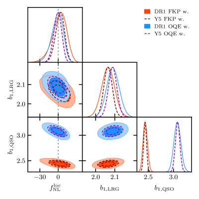
Figure 9: Posteriors in the $(f_{\rm NL}^{\rm loc},b_{1,\textrm{LRG}},b_{1,\textrm{QSO}})$ plane of the combine fit of the mean of power spectrum $(\ell=0,\ell=2)$ over the 1000 realizations of the LRGs and QSOs. $b_{\Phi}(b_{1},p)$ is derived via Eq. 2.6, where $p=1$ for the LRGs and $p=1.6$ for the QSOs. The other parameters are allowed to vary but not shown here. The corresponding MAP values are displayed in Table 5.

Table 5: Results of the fit of the combine mean of power spectrum over 1000 realizations of the LRGs and QSOs. Central values are the best fit values from the minuit minimization while the errors are the $1\sigma$ credible interval from the chains that are displayed in Figure 9. Combining the LRGs and the QSOs leads to a direct statistical gain about 20% compared to the QSOs only.

	$f_{\mathrm{NL}}^{\mathrm{loc}}$	$b_{1,\mathrm{QSO}}$	$s_{n,0,\mathrm{QSO}}$	$\Sigma_{s,\mathrm{QSO}}$	$b_{1,\mathrm{LRG}}$	$s_{n,0,\mathrm{LRG}}$	$\Sigma_{s,\mathrm{LRG}}$
DR1 (FKP)	${5}_{-9.8}^{+13.0}$	${2.437}_{-0.045}^{+0.043}$	${-0.006}_{-0.049}^{+0.056}$	${2.63}_{-0.79}^{+1.36}$	${2.062}_{-0.035}^{+0.032}$	${0.039}_{-0.062}^{+0.066}$	${4.35}_{-0.42}^{+0.54}$
DR1 (OQE)	${1.1}_{-7.9}^{+10.5}$	${3.068}_{-0.072}^{+0.064}$	${-0.031}_{-0.072}^{+0.078}$	${0.0}_{-0.95}^{+0.26}$	${2.087}_{-0.034}^{+0.032}$	${0.022}_{-0.065}^{+0.062}$	${4.35}_{-0.44}^{+0.52}$
Y5 (FKP)	${3.6}_{-6.8}^{+7.6}$	${2.439}_{-0.029}^{+0.028}$	${-0.293}_{-0.036}^{+0.035}$	${3.46}_{-0.46}^{+0.58}$	${2.064}_{-0.022}^{+0.022}$	${0.038}_{-0.044}^{+0.045}$	${4.55}_{-0.31}^{+0.33}$
Y5 (OQE)	${-0.1}_{-6.2}^{+6.8}$	${3.078}_{-0.045}^{+0.044}$	${-0.073}_{-0.049}^{+0.054}$	${0.0}_{-0.70}^{+0.18}$	${2.088}_{-0.022}^{+0.022}$	${0.023}_{-0.046}^{+0.043}$	${4.59}_{-0.29}^{+0.34}$

Due to the shape of the redshift distribution, the OQE weights have a negligible impact on the constraint of $f_{\rm NL}^{\rm loc}$ for the LRGs such that we do not use them in the following, and we only give the result for the use of FKP weights.

4.3 Discrepancy between FKP and OQE weights

As reported in Table 4, in the case of the QSO there is a discrepancy between the measured value of $f_{\rm NL}^{\rm loc}$ between the use of the FKP ($f_{\rm NL}^{\rm loc}\simeq 3$) or OQE ($f_{\rm NL}^{\rm loc}\simeq-3$) weighting schemes. This discrepancy is statistically significant because we are fitting the mean over 1000 realizations, which reduces the expected statistical uncertainty by a factor $\sqrt{1000}\sim 31$. For the LRGs, OQE weights have a minor impact such that the discrepancy does not exist. Although shown in the following, we do not discuss it and only focus in the QSO case.

To investigate this effect, we fit individually the 1000 realizations with the different weighting schemes. First, we check that the standard deviation from the best fit value of $f_{\rm NL}^{\rm loc}$ on the 1000 EZmocks is compatible with the errors given in Table 4. Then, the normalised distribution of the difference between the best fit value of $f_{\rm NL}^{\rm loc}$ with the different weights are shown in Figure 10, where the mean and the standard deviation of each distribution are displayed in the legend.

The shift observed between the FKP and the OQE weights in Table 4 ($-6$) is consistent with the mean ($-5.8$) of the distribution displayed in blue in Figure 10. The shift does not disappear by increasing the data size (blue versus red histogram), however, the standard deviation becomes lower, meaning that the shift seems to be a real bias between the two weighting schemes.

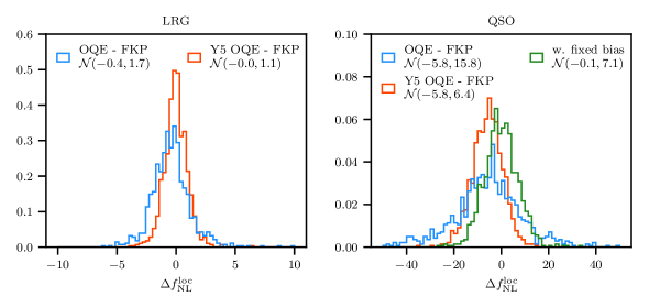
Figure 10: Normalised distribution from individual fit of the 1000 realizations of the difference between the best-fit value of $f_{\rm NL}^{\rm loc}$ obtained with FKP or OQE weights. LRGs are on the left and QSOs on the right. Blue is for DR1, red for Y5 mocks and green is for DR1 but with the bias fixed during the fit. The mean and the standard deviation for each histogram are given in the legend.

The shift between the measurement of $f_{\rm NL}^{\rm loc}$ with the two weighting schemes is lower than the statistical errors, and it is still the case for this first DESI data release ($\sim 0.5\sigma$). However, as shown with the forecast for the Y5 data, this will not be the case with the increase of the data size in the upcoming DESI release. Thus, additional study will be required to avoid biaising the measurement. To investigate, we perform the fit with the linear bias $b_{1}$ fixed for the Y1 mocks and the discrepancy vanished as shown by the green histogram in Figure 10. Hence, a better knowledge on $b_{1}$ could help to obtain an unbiased measurement of $f_{\rm NL}^{\rm loc}$ with the OQE weighting scheme. This could be achieved by increasing $k_{\rm max}$, which, in turn, would require the use of much more complex model than Eq. 2.4 as in [33]. We leave this analysis and improvement for future work.

This discrepancy appears also later when measuring $f_{\rm NL}^{\rm loc}$ from the data. However, the majority of this discrepancy is due to a residual systematics in the lower redshift range of the QSO sample that is under-weighted by the OQE weighting scheme. The difference is $\Delta f_{\rm NL}^{\rm loc}\sim 20$, so that the use of OQE weights is necessary to have an unbiased measurement, see Section 6.

4.4 Radial Integral Constraint

First, the global integral constraint (GIC) [95] is described in Section A.5 and we show that it can be neglected in this analysis.

Up until now, the randoms of the EZmocks were generated in a box in three dimensions such that they already have their proper redshifts. We simply sampled them to match the desired redshift distribution. However, as explained in Section 3.1.2, the redshift of the randoms are drawn directly from the data catalog using the so-called shuffling method [71]. By imprinting the data redshifts into the randoms, radial modes in the measured power spectrum are nulled leading to the so-called Radial Integral Constraint (RIC) [95]. To quantify the contribution of the effect, we apply the shuffling method on the first 100 EZmocks that we use. As illustrated in Figure 11 and in Table 6, the use of the shuffling method without any correction biases the measurement of $f_{\rm NL}^{\rm loc}$ by $1\sigma$ of the statistical uncertainty.

In contrast to [8, 14] which implement an additive correction to account for the radial constraint by taking simply the difference of the power spectrum between the mocks with and without shuffling, we instead provide a multiplicative correction by modifying the window function:

$$\mathcal{W}\rightarrow\mathcal{W}-\mathcal{W}^{\rm RIC}.$$ (4.9)

Hence, the correction does not depend on the value of the power spectrum on which it is estimated.

As described in Section 2.2 of [95], the contribution of the RIC has a similar shape as the global one with additional anisotropy and scale dependence coming in compared to Eq. A.5 such that it may be reasonable to look for:

$$\left(\mathcal{W}^{\mathrm{RIC}}_{\ell\ell^{\prime}}\right)_{ij}=\dfrac{\left(\mathcal{W}_{\ell p}\right)_{im}}{\left(\mathcal{W}_{00}\right)_{00}}\left(f_{pq}\right)_{mn}\left(\mathcal{W}_{q\ell^{\prime}}\right)_{nj},$$ (4.10)

with the summation runs over $p,q,n,m$. $\left(f_{pq}\right)_{mn}$ decreases rapidly with increasing $p,q$, e.g.:

$$\left(f_{pq}\right)_{mn}=A_{pq}\,e^{-(k_{n}^{2}+k_{m}^{2})/\sigma_{pq}^{2}},$$ (4.11)

where $A_{pq}$ and $\sigma_{pq}$ are $2\times(3\times 3)$ unknown coefficients. Note that under this parametrization, one can retrieve the GIC contribution given in Eq. A.5 by setting $\left(f_{00}\right)_{00}=1$ and 0 for the others.

The coefficients $A_{pq}$ and $\sigma_{pq}$ can be estimated with the set of EZmocks with and without the shuffling method. The convolved power spectrum of this EZmocks with the shuffling method can be written as

$$\left(\hat{P}_{\ell}^{\rm shu}\right)_{i}=\left(\mathcal{W}_{\ell\ell^{\prime}}\right)_{ij}\left(\hat{P}_{\ell\prime}^{\rm box}\right)_{j}-\left(\mathcal{W}_{\ell\ell^{\prime}}^{\rm RIC}\right)_{ij}\left(\hat{P}_{\ell\prime}^{\rm box}\right)_{j},$$ (4.12)

where $\hat{P}_{\ell\prime}^{\rm box}$ is the power spectrum from the box used to build the cutsky mock i.e. corresponds to one realization of the underlying $P_{\ell\prime}^{\rm theo}$ used to generate the mocks. The first term of the RHS is the observed power spectrum measured without the shuffling:

$$\left(\hat{P}_{\ell}^{\mathrm{no\;shu}}\right)_{i}=\left(\mathcal{W}_{\ell\ell^{\prime}}\right)_{ij}\left(\hat{P}_{\ell\prime}^{\rm box}\right)_{j}.$$ (4.13)

Due to the large variance during the subsampling to go from the box to the cutsky, we do not want to compare the power spectrum from the box and the one from the cutsky. Fortunately, one can extract the window matrix from Eq. 4.10 such that the RIC contribution can be re-written as

$$\left(\mathcal{W}_{\ell\ell^{\prime}}^{\rm RIC}\right)_{ij}\left(\hat{P}_{\ell\prime}^{\rm box}\right)_{j}=\left(\mathcal{W}_{\ell p}\right)_{im}\left(f_{pq}\right)_{mn}\left(\hat{P}_{q}^{\mathrm{no\;shu}}\right)_{n}.$$ (4.14)

Note that $\left(\mathcal{W}_{00}\right)_{00}$ is a constant, and to simplify, we renormalise $\left(f_{pq}\right)_{mn}$ such that $\left(f_{pq}\right)_{mn}\rightarrow\left(f_{pq}\right)_{mn}/\left(\mathcal{W}_{00}\right)_{00}$ without changing the result.

Finally, the coefficients $A_{pq}$ and $\sigma_{pq}$ in $\left(f_{pq}\right)_{mn}$ can be estimated by minimising the sum over 100 independent realization of a standard $\chi^{2}$ defined for each realization by

$$\chi^{2}=\left(\Delta_{\ell}\right)_{i}^{T}\left(C^{-1}_{\ell\ell^{\prime}}\right)_{ij}\left(\Delta_{\ell^{\prime}}\right)_{j},$$ (4.15)

where $\left(C_{\ell\ell^{\prime}}\right)_{ij}$ is the covariance matrix and $\left(\Delta_{\ell}\right)_{i}$ is given by

$$\left(\Delta_{\ell}\right)_{i}=\left(\hat{P}_{\ell}^{\mathrm{shu}}\right)_{i}-\left(\hat{P}_{\ell}^{\mathrm{no\;shu}}\right)_{i}+\left(\mathcal{W}_{\ell p}\right)_{im}\left(f_{pq}\right)_{mn}\left(\hat{P}_{q}^{\mathrm{no\;shu}}\right)_{n}.$$ (4.16)

The minimization is performed with iminuit and is fitted independently for the FKP or OQE weights and for the different tracers. We use $\ell=0,2,4$ for FKP weights and only $\ell=0,2$ for OQE weights with $0.003~{}h\text{Mpc}^{-1}<k<0.01~{}h\text{Mpc}^{-1}$. As a verification, the minimization was also performed only with the first 50 mocks and tested on the mean of the 50 others, and similar result were obtained.

Note that by definition the GIC is included in the RIC [95]. However, in Eq. 4.16, we used only measured power spectra such that the GIC vanished in $\hat{P}_{\ell}^{\mathrm{shu}}-\hat{P}_{\ell}^{\mathrm{no\;shu}}$ and cannot be modelled with this method. Fortunately, we show in Section A.5 that GIC is negligible for our analysis.

Figure 11 shows the mean power spectrum over the 100 realizations for the LRGs and the QSOs using the shuffling method. The dashed lines are the best fits to the mean power spectrum without the shuffling method, illustrating the radial integral constraint contribution to both the monopole and the quadrupole. The contribution to the monopole can be easily reproduced by decreasing the value of $f_{\rm NL}^{\rm loc}$, while the suppression of the power at large-scales in the quadrupole cannot. Adding the RIC correction enables us to measure $f_{\rm NL}^{\rm loc}$ as shown in Table 6 which compares the result of the best fit with and without the RIC correction to the one without the shuffling method. Not introducing this correction would bias $f_{\rm NL}^{\rm loc}$ by $2/3\sigma$.

To validate this multiplicative correction, we also test the RIC correction on the mean of 30 mocks with a different power spectrum than the ones used to estimate this correction. For this reason, we applied the blinding procedure described in [72] with $f_{\rm NL}^{\rm blind}=20$. As shown in the last row of Table 6, the correction performs well even if the shape of the power spectrum is different, validating the multiplicative correction proposed here.

Finally, the covariance obtained from 100 realizations with the shuffling method is very similar to the one obtained from 100 realizations without it. Thus, in what follows, we always use the covariance estimated from 1000 realizations without the shuffling method as described in Section 3.3.3.

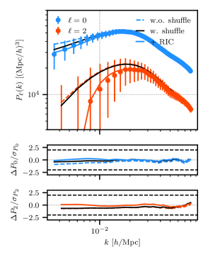
(a) LRG ($0.4<z<1.1$) with FKP.

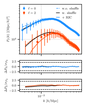
(b) QSO ($0.8<z<3.1$) with FKP.

Figure 11: Multipoles of the mean power spectrum (dotted points), computed with FKP weights, over 100 realizations describing either the DESI DR1 LRGs (left) or QSOs (right) with the shuffling method applied. The errors are from the covariance matrix for the DR1 analysis. The colour dashed lines are the best fits from the realizations without the shuffling method. The black lines are the best fit from the realizations with the shuffling method but without taking into account the radial integral constraint contribution while the solid colour lines are the best fit taking into account this contribution. On the monopole, this contribution can be reproduced by decreasing the value of $f_{\rm NL}^{\rm loc}$, thus needs to be corrected to measure this parameter correctly. Note that the quadrupole ($\ell=2$) has almost no constraining power on $f_{\rm NL}^{\rm loc}$ such that even with the important lack of power at large-scales on the shuffled quadrupole, this does not impact the value of $f_{\rm NL}^{\rm loc}$.

Table 6: Results of the fits using the DR1 covariance matrix on the mean of the power spectrum with FKP weights, with and without the shuffling method and the RIC contribution, over 100 realizations for the LRGs and QSOs and over 30 realizations for the QSOs with the blinding applied ($f_{\rm NL}^{\rm blind}=20$). The central values are best fit values from the minuit minimization while the errors are the $1\sigma$ credible intervals from the chains. Note that the RIC correction for the bottom row is computed from the mocks without the blinding (i.e. the correction is the same for the second and bottom row), validating our multiplicative correction. The systematic error contribution is discussed in Section 6.3.

	parameter	no shuffle	shuffle	shuffle + RIC
DR1 LRG	$f_{\rm NL}^{\rm loc}$	$6_{-12}^{+17}$	$-4_{-13}^{+16}$	$7_{-12}^{+17}$
	$b_{1}$	$2.060_{-0.037}^{+0.032}$	$2.069_{-0.036}^{+0.033}$	$2.055_{-0.035}^{+0.031}$
	$s_{n,0}$	$0.046_{-0.063}^{+0.062}$	$0.058_{-0.070}^{+0.058}$	$0.052_{-0.058}^{+0.064}$
	$\Sigma_{s}$	$4.32_{-0.37}^{+0.52}$	$4.57_{-0.38}^{+0.47}$	$4.42_{-0.39}^{+0.48}$
DR1 QSO	$f_{\rm NL}^{\rm loc}$	$3_{-15}^{+16}$	$-7_{-15}^{+19}$	$6_{-16}^{+14}$
	$b_{1}$	$2.438_{-0.049}^{+0.046}$	$2.451_{-0.054}^{+0.048}$	$2.431_{-0.045}^{+0.047}$
	$s_{n,0}$	$-0.002_{-0.054}^{+0.052}$	$-0.001_{-0.052}^{+0.058}$	$0.004_{-0.050}^{+0.053}$
	$\Sigma_{s}$	$2.67_{-0.78}^{+1.25}$	$2.98_{-0.67}^{+1.20}$	$2.87_{-0.77}^{+1.19}$
DR1 QSO with blinding	$f_{\rm NL}^{\rm loc}-f_{\rm NL}^{\rm blind}$	$8_{-12}^{+13}$	$1_{-12}^{+16}$	$9_{-12}^{+14}$
(RIC from DR1 QSO)	$b_{1}$	$2.406_{-0.043}^{+0.042}$	$2.410_{-0.048}^{+0.043}$	$2.403_{-0.046}^{+0.038}$
	$s_{n,0}$	$-0.011_{-0.048}^{+0.052}$	$0.006_{-0.053}^{+0.051}$	$0.000_{-0.049}^{+0.049}$
	$\Sigma_{s}$	$2.72_{-0.74}^{+1.31}$	$2.99_{-0.65}^{+1.24}$	$2.95_{-0.65}^{+1.26}$

5 Imaging systematics: weights validation

Imaging systematic mitigation aims to correct for the spurious density fluctuations in the angular distribution of the objects from the fluctuation of the imaging quality and foreground across the photometric survey used for the target selection. These fluctuations are illustrated in Figure 12 and in Figure 13 that show the relative density of the number of objects as a function of different templates where the black lines are for the sample not corrected for these dependences.

These systematics represent the most significant source of contamination in measuring the large-scale modes of the power spectrum. Over the past decade [98, 99, 100, 101], mitigating these effects has been a major focus in both galaxy clustering analyses from spectroscopic surveys, as in eBOSS [15, 102, 103, 16], and from photometric surveys as in the Dark Energy Survey (DES) [104, 105]. In Section 5.1, we present the methodology used in DESI and through this paper to compute the imaging systematic weights. Then, in Section 5.2, we use EZmocks to test the impact of different imaging mitigation weighting schemes on $f_{\rm NL}^{\rm loc}$, and compute the angular integral constraint contribution to correct for the use of these weights. Finally, in Section 5.3, we analyse the blinded data and validate the fiducial mitigation method.

5.1 Mitigation of the dependence on the imaging quality of the target selection

5.1.1 Default configuration in DESI

In DESI [70], we follow the commonly applied method based on template fitting that was developed in the last major surveys [106, 107, 15, 108, 109]. This method provides a per-tracer correction weight $w_{\rm sys}$ calibrated from the observed variation of target density as a function of features that describe the imaging qualities. Recently, [15, 16] showed that this method could be improved by introducing some non-linearities between the template using supervised machine learning. Hence, in the following, the imaging weights $w_{\rm sys}$ are estimated at HEALPix level [87] using either a linear or a random forest-based regression with a k-fold training. Note that compared to the one in [70], the linear regression here does not fit the data to binned statistics but rather the fluctuation at HEALPix level. All the weights are computed with regressis as described in [57].

Following [31, 110] that assess the correlation between the target density and the different features, we consider only these 12 observational features:

• Stellar density $[\rm{deg}^{-2}]$ is the density of point sources from Gaia DR2 [111] in the magnitude range: $12<\textsc{\small{PHOT\_G\_MEAN\_MAG}}<17$.

• HI $[\rm{cm}^{-2}]$ is the hydrogen column density from the Effelsberg-Bonn HI Survey (EBHIS) and the third revision of the Galactic All-Sky Survey [112].

• E(B-V) diff GR / E(B-V) diff RZ $[\rm{mag}]$: is the difference between the SFD E(B-V) [113] and the E(B-V) determined from DESI stars spectra [114]. This new method from DESI data produce two values one based on $g-r$ and the other on $r-z$. Note, we are not using the standard E(B-V) map alone since it is strongly correlated to the large scale structure of the Universe via the Cosmic Infrared Background [115].

• PSF Depth $[1/\rm{nanomaggies}^{2}]$ (in $r$, $g$, $z$, $W1$, $W2$) is the 5-sigma point-source magnitude depth.

• Galaxy Depth $[1/\rm{nanomaggies}^{2}]$ (in $r$, $g$, $z$) is an alternative to PSF Depth. It measures the 5-sigma galaxy-source magnitude depth. It is only used instead of the corresponding PSF Depth.

• PSF Size $[\rm{arcsec}]$ (in $r$, $g$, $z$): Inverse-noise-weighted average of the full width at half maximum of the point spread function, also called the delivered image quality.

As in [31], the default configuration for the LRG sample is to compute the imaging weights in three different redshift bins ($0.4<z<0.6$, $0.6<z<0.8$ and $0.8<z<1.1$) and on three independent photometric regions (North, South (NGC), South (SGC) + DES) with the following features:

• $0.4<z<0.6$: Stellar density, HI, PSF Size $r$, Gal Depth $z$ / $r$, PSF Depth $W1$,

• $0.6<z<0.8$: Stellar density, HI, PSF Size $r$, Gal Depth $z$ / $g$, PSF Depth $W1$,

• $0.8<z<1.1$: Stellar density, HI, PSF Size $r$ / $z$, Gal Depth $z$, PSF Depth $W1$.

The default configuration for the QSO sample is also to compute the weights in three redshift bins ($0.8<z<1.3$, $1.3<z<2.1$ and $2.1<z<3.1$) and in three photometric regions (North, South (NGC) + South (SGC), DES) of but considering the same features in each bin:

• $0.8<z<1.3$ / $1.3<z<2.1$ / $2.1<z<3.1$: Stellar density, HI, E(B-V) diff GR / RZ, PSF Depth $r$ / $g$ / $z$ / $W1$ / $W2$, PSF Size $g$ / $r$ / $z$.

These redshift bins were designed to match the redshift ranges of the sample used for the BAO or RSD measurements, except for the additional split for the QSOs at $z=1.3$.

This additional split was motivated by the lack of QSOs with small redshift ($z<1.3$) in the regions where the PSF Depth is higher, as noted in [54]. Indeed, QSOs that are sufficiently close to us are increasingly identified as extended sources in regions with high PSF depth, leading to their rejection during the target selection. This effect is limited to the low-$z$ end of the QSO sample and is not apparent when using the broad redshift bin of $0.8<z<2.1$. However, it contributes to an excess of power on large scales in the power spectrum if it is not properly addressed as shown in Section A.6.

In our template-fitting methodology, we assume that a template is fixed across the redshift bin (but allowed to vary between different bins). Hence, we are not able to model any redshift dependence inside a redshift bin. Note that this could also be useful for LRGs as found in [110] . A more detailed analysis, which we leave for the future, might want to allow the template weights to vary within the redshift bins of individual tracers.

5.1.2 Test with other configurations

To assess the efficiency of the imaging systematic mitigation, we test several modifications of the default configuration. In particular, for the LRGs, we alternately adopt:

• Default: Default configuration, as described in Section 5.1.1, computed either with a random forest using either $N_{\rm side}=128$ or $256$ or with a Linear regression using $N_{\rm side}=256$.

• PSF Depth: Default with a linear regression using $N_{\rm side}=256$, where the Gal Depth features are switched with the PSF Depth features.

• Same Feature Zbin: Using all the features for each redshift bins: Stellar density, HI, E(B-V) diff GR / RZ, PSF Size $r$ / $z$, Gal Depth $z$ / $r$, PSF Depth $W1$. We test the linear regression using either $N_{\rm side}=128$ or $256$.

• With DES: as Default, but the regression is performed independently in (North, South, DES) instead of (North, South (NGC), all the SGC) with a linear regression using $N_{\rm side}=256$.

• 4 regions: as Default, but the regression is performed independently in (North, South (NGC), South (SGC), DES) instead of (North, South (NGC), all the SGC) with a linear regression using $N_{\rm side}=256$.

For the QSOs, we test:

• Default: Default configuration computed either with a random forest with $N_{\rm side}=256$ or with a Linear regression using either $N_{\rm side}=128$ or $256$.

• No PSF Size: Default with a linear regression using $N_{\rm side}=128$ where the PSF size features in the $g$, $r$, $z$ bands are all removed.

• No PSF Depth: Default with a random forest regression using $N_{\rm side}=128$ where the PSF depth features in the $g$, $r$, $z$, $W1$ and $W2$ bands are all removed.

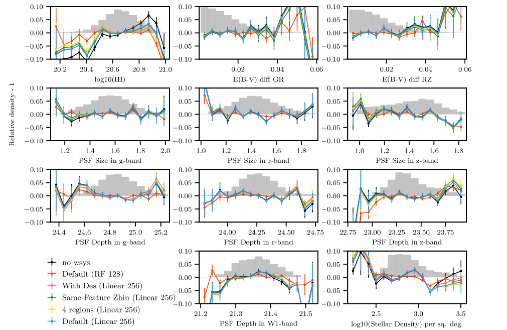
Figure 12: Relative density centered around 0 as a function of the amplitude of several observational features of the LRGs (0.6 < z < 0.8) in the South (SGC) region. Back lines are without the imaging systematic correction while the different colours are for the different corrections (RF regression in red, Linear in blue/green). The histogram represents the fraction of objects in each bin for each observational feature and the error bars are the estimated standard deviation of the normalised density in each bin.

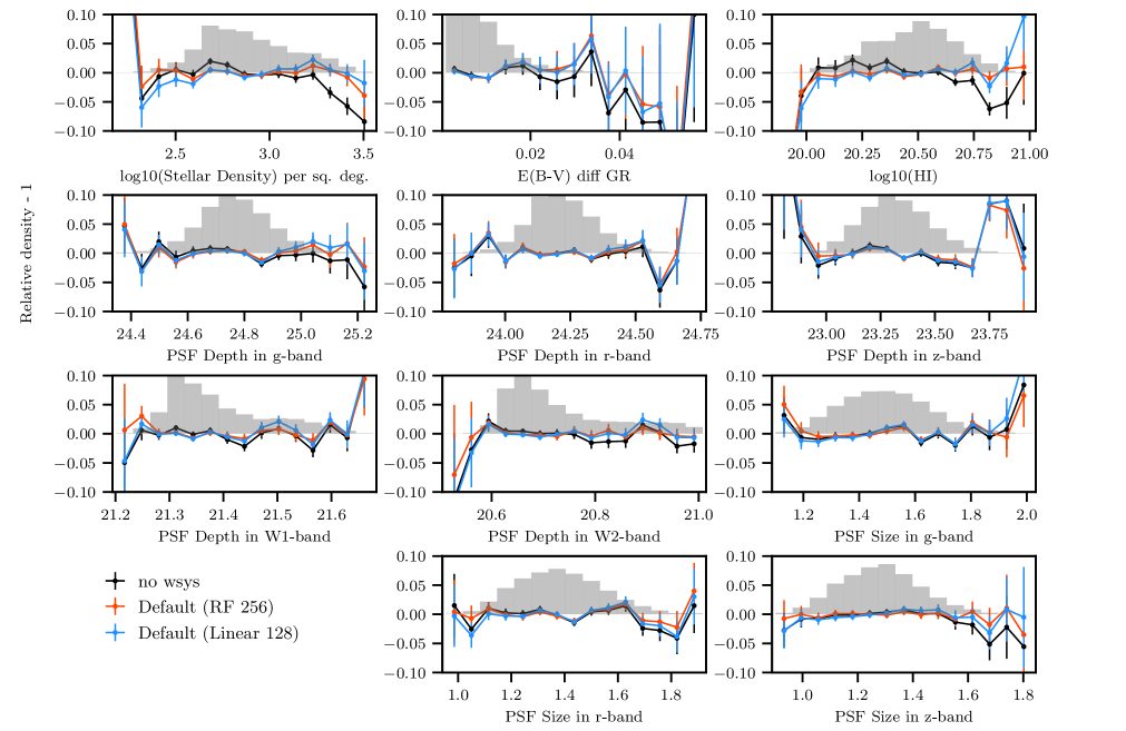
Figure 13: Same as Figure 12 but for the QSOs (1.3 < z < 2.1) in the South (NGC).

The efficiency of some of these variants is shown in Figure 12 for the LRG ($0.6<z<0.8$) sample in the South (SGC) region and in Figure 13 for the QSO ($1.3<z<2.1$) sample in the South (NGC) region. These plots show the relative density of the objects as a function of the amplitude of the templates corresponding to different features. The black lines are without any imaging systematic weights while the different colours are when we apply the different weights computed with the configurations explained above. Similar plots for the other regions and other redshift sub-samples were also used to assess the efficiency of the different corrections.

All the configurations using the linear regression, even if not shown in these figures for clarity, give very similar results. The most important difference appears when we use the non-linear regression (red lines) instead of the linear one (blue lines). However, as noted in [16, 57, 17], non-linear regressions have more degrees of freedoms to "flatten" the black line such that it does not necessarily result in a better correction. In addition, this additional degree of freedom leads to a modification of the power spectrum at large scales as illustrated in the next section.

5.2 Angular Integral Constraint

To compare the efficiency of the different imaging systematics, we first need to quantify their impacts on mocks without any contamination. Then, if necessary, we need correct for the angular integral constraint that appears due to the use of these weights.

5.2.1 Illustration with the EZmocks

As shown in [17], allowing too much flexibility with a neural network during regression results in significant removal of large-scale power in the monopole that strongly biases the measurement of $f_{\rm NL}^{\rm loc}$. To address this, we first perform a null test, by using our set of EZmocks that does not contain any imaging systematic contamination. Doing so, the mock density of tracers (either QSOs or LRGs) is strictly uncorrelated (when averaging over many realizations) with the different imaging features presented in Section 5.1. Hence, the imaging systematic mitigation i.e. the computation of the per-tracer weights $w_{\rm sys}$ from linear or random forest regression, should not bias $f_{\rm NL}^{\rm loc}$. Any observed impact on the power spectrum measurement is then attributable to the methodology itself and must be corrected to prevent bias in our results.

From the different setups described above, we can compute the per-tracer correction weights $w_{\rm sys}$, to be used in the power spectrum estimator through Eq. 3.1. We measure the power spectrum monopoles as the mean computed over the first 30 EZmocks, for the LRGs and QSOs to isolate and quantify the impact of the imaging systematic weights. The impact on the monopole of these different configurations are shown in Figure 14 where we displayed the relative difference between the monopoles estimated with and without imaging systematic weights divided by the DR1 statistical errors. The regression using the random forest is displayed in red, while the linear regression in blue. From Figure 14, it is clear that the random forest-based regression biases negatively the estimation of the monopole for either QSOs or LRGs compared to the linear regression, whose effect is smaller. This is because the regression has enough freedom to completely homogenise the angular distribution at a specific $N_{\rm side}$, nulling a lot of large cosmological angular modes. By removing physical modes on the large scales, random forest-based mitigation biases negatively the measurement of $f_{\rm NL}^{\rm loc}$, while the linear regressions has a relatively small impact.

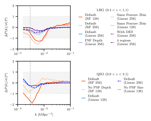
Figure 14: Relative difference between the power spectrum monopoles obtained using FKP weights with and without imaging systematic weights to the DR1 statistical errors derived from the 1000 EZmocks. Each monopole that we show represents the mean computed from 30 realizations. LRGs are on the top and QSOs are on the bottom. The blue (resp. red) lines are for linear (resp. Random Forest) regressions while the specificity for each regression is explained in the text. The resulting values of $f_{\rm NL}^{\rm loc}$ are displayed in Figure 15 and given in Table 14.

To quantify the bias introduced on $f_{\rm NL}^{\rm loc}$ measurement, we fit the mean of the power spectrum using the associated DR1 covariance matrix. The best fit for LRGs and QSOs using either FKP or OQE weights are displayed in Figure 15. The Random Forest-based regression introduces an important negative bias in the estimation of $f_{\rm NL}^{\rm loc}$. Indeed, by construction, these weights tend to flatten the angular density at the level of the difference pixels used during the regression, thus canceling modes that are in common between the different pixels. In the QSO case, the OQE weights help to prevent this effect by over-weighting the high-$z$ objects since at higher redshift the angular modes, nulled out by the use of imaging weights, are physically larger and so impact lower $k$’s. For the same reason, this effect is less important for the QSOs than for the LRGs.

Although less statistically significant than the random forest mitigation, this bias exists also in the case of the linear regression. One can reduce it by reducing the number of features used in the fit, as is already the case for the LRGs’ default configuration compared to Same Feature Zbin. However, reducing the number of features can also reduce the efficiency of the weights by not including a feature that actually describes a remaining imaging systematic. A correction in this regard is proposed in Section 5.2.2.

To be conservative and have less significant correction of the effect illustrated in Figure 14, we choose in the following as fiducial weight Default (Linear 256) for the LRGs and Default (Linear 128) for the QSOs. Establish the correction of this effect is the topic of the following section.

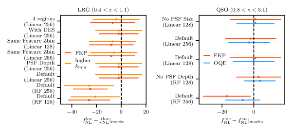
Figure 15: Best fit values of $f_{\rm NL}^{\rm loc}$ with different imaging weights where the value from the EZmocks without weight is subtracted. Red whiskers denote the scenario of using FKP weights, while blue whiskers denote the OQE weights case. For the LRG, red is for $k_{\rm min}=0.003~{}h\text{Mpc}^{-1}$ and orange for $k_{\rm min}=0.006~{}h\text{Mpc}^{-1}$. The impact of the imaging weights on the power spectrum is shown in Figure 14. The values are given in Table 14.

5.2.2 Estimation of the Angular Integral Constraint

The suppression of power in Figure 14, introduced by the imaging systematic weights, can be seen as an Angular Integral Constraint (AIC) [95]. Indeed, the imaging systematic weights aim to remove the angular fluctuations of the density at a pixel level, nulling out some angular modes and reducing the power at large scales. Hence, this effect can be taken into account by adding its contribution to the window matrix:

$$\mathcal{W}\rightarrow\mathcal{W}-\mathcal{W}^{\rm RIC}-\mathcal{W}^{\rm AIC},$$ (5.1)

where $\mathcal{W}^{\rm AIC}$ can be estimated using the same method introduced in Section 4.4. We choose to use the same shape for the $\left(f_{p,q}\right)_{m,n}$ coefficients than for the RIC contribution. Note the $\mathcal{W}^{\rm AIC}$ is estimated with the realization of mocks without the shuffling method i.e. without the RIC contribution, so that the AIC and RIC contributions is added linearly in the total window function. However, one can imagine, in the future, to model the two contributions simultaneously.

It is impossible to correctly quantify the efficiency of the imaging systematic mitigation on the power spectrum without taking into account the AIC correction. First, for the QSO and LRG fiducial weights that use linear regression, and second, for the weights that use random forest-based correction and either more features (for the LRGs) or a better $N_{\rm side}$ resolution (for the QSOs). Following the same methodology as in Section 4.4, the $\mathcal{W}^{\rm AIC}$ correction is estimated from the first 30 EZmock realizations on which the weighting scheme is applied.

To test the impact of the AIC correction on parameter constraints, we fit the mean of 30 uncontaminated EZmock power spectra, each of them estimated with the imaging mitigation weighting schemes to be tested. The best fits using (red points) or not (blue points) the AIC correction in the parameter fit are given in Figure 16. First, even if the contribution is very small ($\sim 0.4\sigma$) for the linear-based weights, it exists, biasing the result, however, can be corrected. In all configurations, taking into account the AIC contribution enables us to recover the expected value of $f_{\rm NL}^{\rm loc}$ that is measured from the realization without the weighting scheme applied (first column). Our correction is slightly worse for the random forest-based weights but is enough to quantify the efficiency of weights.

In the following, we neglect the impact of the AIC on the covariance matrix since it is too numerically expensive to run for the different $w_{\rm sys}$ configuration as many power spectra.

Note that the angular integral constraint is purely geometrical and does not reflect the efficiency of the imaging weights, meaning it can be reliably estimated using uncontaminated simulations. In the following, all the fits presented contain both the radial and the angular integral constraint contribution into the window matrix.

Figure 16: Best fit values of ($f_{\rm NL}^{\rm loc}$, $b_{1}$) without (blue) and with (red) the angular integral constraint contribution into the window function for different imaging weights where we have substracted the value from the EZmocks without imaging systematic weights. The values are given in Table 15. The systematic error contribution is discussed in Section 6.3.

5.3 Validation with the blinded data

Following the analysis in [62] and supported by the results on EZmocks (Section 5.2.1), our fiducial analyse uses the Default (Linear 256) weights for the LRGs and the Default (Linear 128) weights for the QSOs. In Section 5.3.1, we check the internal consistency of the default configurations for LRG and QSO. From this, we identifiy possible remaining systematics that we explore through extended mitigation methods in Section 5.3.2. Finally, we check the robustness of the $f_{\rm NL}^{\rm loc}$ measurement from blinded data in Section 5.3.3.

5.3.1 Search for residual systematics

First, we can assess the efficiency of the default configurations for imaging systematic mitigation by examining the compatibility between the blinded large-scale modes in the monopole, which are measured in different photometric regions and redshift bins. This is possible because, as shown in [72], the blinding is not sensitive to the variation of the shot noise in the sample, and therefore is the same across the different redshift bins and photometric regions. Note also that RIC and AIC contributions to the window and the window matrix itself are different for each sub-sample either for the redshift or photometric region split, such that the very large scales should be different. Hence, the aim of this section is not to quantify the agreement of the different sub-samples, but only to look for any spurious excess of power at large scales resulting from a remaining systematic.

In the following, we measure LRG and QSO blinded power spectrum monopoles separately in the different redshift bins detailed in Section 5.1, as well as in the three different photometric regions, North, South (NGC) and South (SGC). As an indication of the statistical significance of the different photometric regions compared to the complete sample, the effective area for the DESI DR1 LRGs and QSOs are (in $\%$):

• North: $(18,20)$,

• South (NGC): $(48,44)$,

• South (SGC): $(25,27)$,

• DES: $(9,9)$.

The DES region is the smallest region, while South (NGC) is the most important one. These differences in effective areas are visible in Figure 1. To assess the statistical significance of each redshift bin, one can look at the redshift distribution shown in Figure 2. From this, we note that DES has a very low statistical significance compared to others. Then, using the fiducial imaging mitigation weighting schemes, these monopoles are shown in Figure 17(a) (resp. in Figure 17(b)) for the LRGs (resp. for the QSOs).

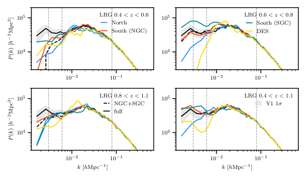
(a) DESI DR1 LRG (blinded)

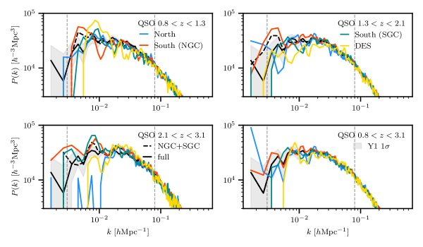
(b) DESI DR1 QSO (blinded)

Figure 17: Monopole of the power spectrum, measured with the fiducial $w_{\rm sys}$, of the blinded LRG (top panels) and blinded QSO (bottom panels) samples for different redshift bins and the different photometric regions (North in blue, South (NGC) in yellow, South (SGC) in green and the DES region in red). For each redshift bin, the black dashed line is the monopole measured on the entire footprint, while the solid black line is the monopole measured on the full redshift range and the entire footprint. The bottom right plot in each set of panels gives the monopole from the full redshift range on the different photometric regions. The gray region for each panel is the $1\sigma$ deviation from the EZmocks with the full redshift range and the entire footprint. The vertical grey dashed lines depict the scale range used for the fit.

For the LRGs (Figure 17(a)), the shape of the monopole for the full sample (black line) exhibits a unusual shape at very large scales ($k\sim 0.003~{}h\text{Mpc}^{-1}$). We also note a relatively strong discrepancy at these scales between the monopole from the different photometric regions (bottom right panel). In addition, this discrepancy around these scales is the most important for the middle redshift bins (top right panel) where South (SGC) region shows an unexpected excess of power. This could be due to residual systematic contamination that the current default weight do not remove. For the two other redshift bins (top and bottom left panel), the monopoles agree with each other, and with the one from the entire footprint (black dashed lines), such that no clear remaining systematics appear in these bins.

In Section 5.3.2, we investigate different imaging weights to remove this excess of power. However, we note that increasing the minimal scale from $k_{\rm min}=0.003~{}h\text{Mpc}^{-1}$ to $k_{\rm min}=0.006~{}h\text{Mpc}^{-1}$ helps to reduce the discrepancy between the different photometric regions in Figure 17(a) (middle gray dashed lines) such that it can be a conservative approach.

In contrast to the case of LRGs, the results for the QSO monopole show a remarkable consistency between the different regions of the sky, for each redshift ranges (Figure 17(b)). In nearly each case shown in the Figure, the results agree within 1$\sigma$ of the monopole evaluated from the full footprint. We observe no spurious signals at large scales. We do observe some deviations in the highest redshift bins $2.1<z<3.1$ (lower left panel) for the North and the DES regions, however, this bin has much less statistical information than the full range and these two regions have a much smaller footprint and completeness compared to the South (NGC/SGC), such that the measurement is still compatible and does not raise any significant concern.

5.3.2 Validation of the imaging systematic weights

In this section, we aim to validate the default weighting scheme as the best choice for correcting imaging systematics for the QSOs and to improve the correction on the LRGs. To quantitatively assess the full imaging systematics mitigation procedure, we compare the measurement of $f_{\rm NL}^{\rm loc}$ for the different imaging weight configurations with the corresponding AIC contribution that we compute for each different setups (see Section 5.2.2), rather than looking at the power spectrum level which do not inform us about due to the different integral constraints.

The blinded $f_{\rm NL}^{\rm loc}$ constraints using the different imaging systematic weights are shown in Figure 19. To assess the importance of the imaging weights, we also include the best fit when no imaging weights are used. Note that all fits, except when no weight is applied, incorporate the AIC contribution into the window matrix, requiring the computation of this contribution for each case. For the LRGs, we show the blinded constraints for two minimal scale cuts: $k_{\rm min}=0.003~{}h\text{Mpc}^{-1}$ or $k_{\rm min}=0.006~{}h\text{Mpc}^{-1}$.

We explore whether new regression methods and/or new set of templates can solve the remaining systematics highlighted in the previous subsection for the LRG sample. The relative density of LRGs ($0.6<z<0.8$) in South (SGC) region as a function of the most relevant observational features are displayed in Figure 12. As mentioned in the introduction of this section, the aim of the imaging systematic weights is to mitigate the trend in the black lines by flattening them. We show the corrected densities using five different imaging mitigation weighting schemes: Default (Linear 256) in blue (our default mitigation method), Default (RF 256) in red, Same Feature Zbin (Linear 256) in green, With Des (Linear 256) in pink, and 4 regions (Linear 256) in gold. While the first three configurations use the entire SGC footprint (South (SGC) + DES) for the regression, the fourth one uses the entire South footprint (South (NGC) + South (SGC)) and the last one only South (SGC). These different setups were tested with uncontaminated EZmocks, where the details can be found in Section 5.1.2. Here, we show only one subregion of one redshift bin for simplicity, but the others have similar behavior.

Except for the RF weights, the four other (linear) corrections provide very similar results and have only a slight impact on the relative density although we have increased the number of templates or isolated the zone in the regression. The impact on the power spectrum of the full sample is shown in Figure 18 where only the RF weights appear to have a significant impact. However, as explained in Section 5.2, one needs to take into account the angular integral constraint that is different for which weights. With this contribution the differences between the RF and the other linear weights in Figure 12 or in Figure 18 are mostly due to this contribution. Indeed, when fitting $f_{\rm NL}^{\rm loc}$ with the AIC contribution, we find roughly the same amount of $f_{\rm NL}^{\rm loc}$, see Figure 19.

In particular, all the weights tested here provide only a minor correction and do not eliminate the apparent excess power at large scales described in Section 5.3.1 at very large scales. We note also that the errors on $f_{\rm NL}^{\rm loc}$ obtained with $k_{\rm min}=0.003~{}h\text{Mpc}^{-1}$ for the different weighting schemes are smaller than expected from the mean of the EZmocks. This discrepancy may indicate the presence of a non-physical signal at these scales.

Hence, we resort to adopting a conservative approach to avoid any bias in our measurement by increasing the minimal scale from $k_{\rm min}=0.003~{}h\text{Mpc}^{-1}$ to $k_{\rm min}=0.006~{}h\text{Mpc}^{-1}$. This change improves the compatibility between the different regions and redshift bins and provides compatible errors between blinded data and simulations. As shown in Section A.2, at this new $k_{\rm min}$ the impact of imaging systematic weight is rather small. Note that with this new minimal scale cut in our LRG fit, the constraint on $f_{\rm NL}^{\rm loc}$ is degraded by about $\sim 30\%$ for the LRGs alone and $\sim 6\%$ when the LRGs are combined with the QSOs compared to the previous minimal scale cut.

Finally, the different configurations provide a consistent measurement of $f_{\rm NL}^{\rm loc}$ with differences relative to the truth of $\Delta f_{\rm NL}^{\rm loc}\sim 4$, and uncertainties $\sigma(f_{\rm NL}^{\rm loc})\sim 18$, illustrating the fact that the default configuration mitigates already all the effect that could be explained by our set of templates. Since none of the new configuration improve the statistical uncertainty of the measurement of $f_{\rm NL}^{\rm loc}$, we decide to use Default (Linear 256) to be aligned with the recommendation of [70] and to avoid strong dependence on the AIC correction (see Table 14). In this way we reduce our measurement’s sensitivity to a mismatch of the AIC estimation.

For the QSOs, we have conducted tests by using different sets of templates and/or regression methods. We showed in Figure 13 the uncorrected/corrected overdensities as a function of different imaging features for QSOs ($1.3<z<2.1$) in South (NGC) for the two configurations: Default (Linear 256) in blue (our default configuration) and Default (RF 256) in red. The impact of these weights on the power spectrum is shown in Figure 18, while the measurement of $f_{\rm NL}^{\rm loc}$ for the different configurations (again using their respective AIC corrections) is given in Figure 19. The deficiency of power at large scales when using Default (RF 256) is not a sign of a better correction since one needs to include the AIC contribution, as explained in Section 5.2. In this case, the use of Default (RF 256) leads to a measurement similar to Default (Linear 256). We note that removing the PSF Depth templates increases a lot the value of $f_{\rm NL}^{\rm loc}$ with the FKP weights. This is expected since these templates explain, for instance, the lack of true QSO at low-z which motivated the additional redshift split at $z=1.3$, see Section A.6. However, not using these templates has a very small impact for the measurement with OQE weights. That can be explained by the fact that these templates describe a systematic at low-$z$ that is under-weighted by the OQE weights and therefore does not impact the measurement.

Moreover, we found a tension between OQE and FKP results that cannot be explained by the small discrepancy found in Section 4.3. Again, since OQE down-weights the low-$z$ QSO sample compared to FKP, the tension can be explained by the presence of an unresolved systematic effect; we will address this point in the next section.

As for the LRGs, to reduce our sensitivity to the AIC correction, we decide to use Default (Linear 256). This is different from [70] who use Default (RF 256).

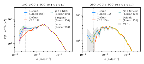
Figure 18: Monopole of the power spectrum measured on the blinded data (LRG on the left and QSO on the right) with FKP weights and different imaging systematic weights. The gray region is the standard deviation from the 1000 EZmocks around the blue lines that are our fiducial choice. Since we need do include the angular integral constraint in the model, the very large-scale modes cannot be compared directly in this figure. The best fit values are displayed in Figure 19.

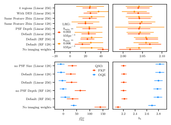
Figure 19: Best fit values of $(f_{\rm NL}^{\rm loc},b_{1})$ for the DR1 blinded LRGs with two values of $k_{\rm min}$ and for the blinded QSOs using either FKP and OQE weights, for various configurations of imaging weights. All the fits include the radial and angular integral constraint contributions. The errors and the central values are from the minimization performed with iminuit and the covariance matrix is the one from the 1000 EZmocks. Note that the errors obtained on $f_{\rm NL}^{\rm loc}$ for the blinded LRGs with $k_{\rm min}=0.003~{}h\mathrm{Mpc}^{-1}$ are too small compared to the expected on from the mean of EZmocks, see Table 4. The configuration chosen for the unblinded analysis is Default (Linear 256) for LRGs and Default (Linear 128) for QSOs. The table reporting the numbers are given in Table 16. The systematic error contribution is discussed in Section 6.3.

5.3.3 Robustness of the measurement

Before measuring $f_{\rm NL}^{\rm loc}$ from the data without blinding, we assess the robustness of our analysis by testing several variations of our fiducial choices i.e. by measuring $f_{\rm NL}^{\rm loc}$:

• from NGC and SGC power spectra separately compared to the fiducial NGC+SGC measurements,

• using the tracers in smaller redshift intervals,

• fitting the power spectra in different $k$-ranges either by increasing $k_{\rm min}$ from $0.003$ (resp. 0.006) for QSOs (resp. for LRGs) to $0.008~{}h\text{Mpc}^{-1}$ or increasing $k_{\rm max}$ from $0.08$ to $0.1~{}h\text{Mpc}^{-1}$.

Note that we occasionally observe biases on $f_{\rm NL}^{\rm loc}$ with the increasing $k_{\rm max}$ for the LRGs, where we may need to include perturbative theory instead of the linear power spectrum as well as non-linear galaxy bias model [116].

For each case, the window matrix $\mathcal{W}$, the RIC contribution $\mathcal{W}^{\rm RIC}$ and the AIC contribution $\mathcal{W}^{\rm AIC}$ are computed following the description given above in Section 5.2.2. For the separate NGC/SGC fits, the covariance is estimated with the EZmocks in the corresponding photometric region. However, the covariance for the two redshift sub-samples is approximated by the full sample covariance matrix, re-scaled by the ratio of the full and sub-sample effective volumes. The effective volume is computed with

$$V_{\mathrm{eff}}=\int\left(\frac{n\left(z\right)P_{0}}{1+n\left(z\right)P_{0}}\right)^{2}\differential V\left(z\right),$$ (5.2)

where for simplicity we use a fixed value for $P(k,z)=P_{0}$ which we evaluate at the effective redshift and at the turnover scale of the power spectrum. It is computed at the effective redshift of the sample and at the turnover of the power spectrum.

The effective volume of the different sub-samples is given in Table 7. Hence, for the LRGs ($0.4<z<0.8$) (resp. $0.6<z<1.1$), the full covariance matrix is rescaled by $\sim 2.1$ (resp. $\sim 1.2$). For the QSOs ($0.8<z<2.1$) (resp. $1.6<z<3.1$), the full covariance matrix is rescaled by $\sim 1.3$ (resp. $\sim 1.8$). We also need to compute the specific effective redshift for these sub-samples; they are given in Table 7. The result of the different posteriors over the $f_{\rm NL}^{\rm loc}-b_{1}$ parameter space are displayed in Figure 20 (we give the values in the appendix, see Table 17).

Table 7: Effective volume computed with Eq. 5.2 and effective redshift with Eq. 3.19 for the sub-sample of the LRGs and QSOs. For the OQE weights, we give only, for simplicity, the effective redshift for the monopole and $p=1.6$.

		$V_{\mathrm{eff}}~{}[(\mathrm{Gpc}/h)^{3}]$	$z_{\mathrm{eff}}$ (FKP)	$z_{\mathrm{eff}}$ (OQE - $\ell=0$)
LRG	$0.4<z<1.1$	$6.5$	0.733	-
	$0.4<z<0.8$	$3.1$	0.601	-
	$0.6<z<1.1$	$5.3$	0.831	-
QSO	$0.8<z<3.1$	$8.3$	1.651	2.082
	$0.8<z<2.1$	$6.4$	1.441	1.691
	$1.6<z<3.1$	$4.6$	2.087	2.236

For the LRGs, we conducted the different robustness tests for the full sample ($0.4<z<1.1$) in Figure 20(a). We find that the posterior is bimodal for the low-$z$ sub-sample ($0.4<z<0.8$) compared to the high-$z$ sample posterior which is Gaussian. This is not expected based on results from simulations. Such discrepancy between the low-$z$ and high-$z$ samples is most likely due to residual systematics in the mitigation of imagining systematics. In addition, we note that the result does not appear to be robust when decreasing $k_{\rm min}$.

Alternatively, we can focus on the high-$z$ sub-sample, whose robustness tests are repeated and displayed in Figure 20(c). When repeating these tests, the fits are more robust when varying the fiducial configuration than for the full sample. Since the effective redshift of the high-$z$ sub-sample is higher, the linear bias is higher such that the constraining power on $f_{\rm NL}^{\rm loc}$ remain relatively unchanged, even if the covariance matrix is properly rescaled by the ratio of the two effective volumes. Accordingly, one can restrict our baseline analysis to the high-$z$ sub-sample without degrading our measurement of $f_{\rm NL}^{\rm loc}$, and in what follows, this is what we do to avoid any potential bias that could come from the low-$z$ sub-sample.

For the QSOs using FKP weights (see Figure 20(b)), we find a good consistency between the NGC and SGC constraints, emphasising the robustness of our mitigation of imaging systematics in the different photometric regions. Moreover, the $k_{\rm min}$ and $k_{\rm max}$ robustness tests are fairly compatible, as our model of linear bias is consistent at these scales for QSOs. However, the low-$z$ ($0.8<z<2.1$) sub-sample and the high-$z$ ($0.8<z<3.1$) sub-sample prefer two different values of $f_{\rm NL}^{\rm loc}$, even though they are statistically compatible, while the full sample prefers a value between the two. Since imaging systematics only add power, this slight tension on $f_{\rm NL}^{\rm loc}$ may indicate a residual unknown systematic in the low-$z$ sample.

Fortunately, we can remove this potential systematic at low-$z$ thanks to the use of the OQE weights that drastically under-weight the low-$z$ object, see Figure 3. The robustness tests for the OQE weights, see Figure 20(d), show excellent agreement even better than when we use the FKP weights, except for the low-$z$ sub-sample part that is now clearly biased. We note also that, the difference between $f_{\rm NL}^{\rm loc}$ from FKP or OQE measurement is much more in agreement when considering only the high-$z$ sub-sample: $\Delta f_{\rm NL}^{\rm loc}=11$ that is statistically acceptable regarding Figure 10, compared to $\Delta f_{\rm NL}^{\rm loc}=37$ when comparing the full sample. For these reasons, we consider OQE weights and the Default (Linear 128) mitigation option to analyse QSO unblinded data.

Moreover, for the QSO sample, we obtain in Figure 20 a lower bias than expected. We measured the linear bias as in Section A.1 from the 2-point correlation function, and we also obtained a lower bias that is compatible to the one measured here. The problem seems to come from the blinded data itself, and we do not investigate this further since the bias obtained with the unblinded data is compatible with the one from eBOSS.

Finally, the decisions took in this section are based on the robustness tests from the blinded data, such that are insensitive to any confirmation bias, and can be used as our fiducial confirmation in the following.

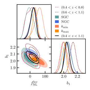
(a) Blinded LRG (FKP).

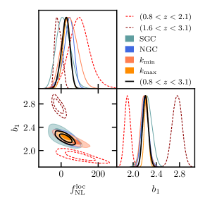
(b) Blinded QSO (FKP).

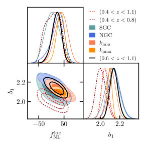
(c) Blinded LRG (FKP) high-$z$.

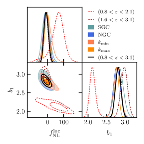
(d) Blinded QSO (OQE).

Figure 20: Posteriors in the $(f_{\rm NL}^{\rm loc},b_{1})$ plane for the blind analysis applied to real data with different modifications around our fiducial choices. We show QSO with FKP (top right) and with OQE (bottom right), as well as the LRG (top left) and the high-$z$ ($0.6<z<1.1$) LRG (bottom left). In each panel, the fiducial choice is displayed in black, while the redshift sub-samples are with dashed lines, and in full colors the measurement using only a part of the footprint or with the modification of the fitting ranges. For the LRGs, the posteriors for the different redshift range are the same in (a) and (c). The parameters $s_{n,0},\Sigma_{s}$ are free during the MCMC but are not shown for better visibility. The corresponding MAP values are given in Table 17.

6 Primordial non-Gaussianity measurement

The model validation done in Section 4 and the data analysis performed with the blinding scheme in Section 5 lead to no relevant systematic bias in our methodology, see Section 6.3 for the quantification of the systematic errors. Therefore, we can measure confidently $f_{\rm NL}^{\rm loc}$ from the unblinded data of the DESI DR1 LRG and QSO samples. We remind the reader that the fiducial choices for our analysis are given in Table 8.

Table 8: Summary of the fiducial choices that we used to fit the unblinded LRG and QSO sample.

	LRG	QSO
weighting scheme	FKP	OQE
$z$ range	$0.6-1.1$	$0.8-3.1$
$z_{\rm eff}$	$0.831$	$2.082$
$k_{\rm min}$ [$h\text{Mpc}^{-1}$]	0.006	0.003
$k_{\rm max}$ [$h\text{Mpc}^{-1}$]	0.08	0.08
$w_{\rm sys}$ (Section 5.1.1)	Default (Linear 256)	Default (Linear 128)

Before we proceed, we draw the reader attention to the fact that several versions of the clustering catalogues were built as described in [70]. The last version with the blinding is v1.2, and this is the version used for all the tests in Section 5. Here, for the unblinded measurement, we are using v1.5, the last version available, and the one used for RSD measurement in [33]. The differences between the versions are described in Appendix B of [70], and we note no relevant change for our analysis between the unblind catalogues from v1.2 and v1.5.

6.1 Consistency validation with the unblinded data

We perform the same tests as in Section 5.3.3 but with the unblinded data, to check the internal consistency of the data. The best fit values are given in Table 9, and the associated posteriors for $(b1,f_{\rm NL}^{\rm loc})$ are given in Figure 21 for the different samples and weighting scheme.

Similar to our conclusions raised with blinded measurements, there are no major differences for the QSO case displayed in Figure 21(b), and the discrepancy between the low-$z$ and high-$z$ sample still exists. However, we note one unexpected minor change: the linear bias measured in the blinded catalogues is lower than that measured in the unblinded ones. Note that the blinding method described [72] does not create a such large bias modification, and we do not know what is the reason of this difference. This has a direct consequence on the error bars that we have in Table 9 compared to Table 17 as the errors are smaller.

We observe that the high-redshift QSO sample provides an unexpectedly stronger constraint on $f_{\rm NL}^{\rm loc}$ relative to the use of the full sample with $\sigma(f_{\rm NL}^{\rm loc})=8.4$ instead of $\sigma(f_{\rm NL}^{\rm loc})=11.5$, and despite the use of the OQE weights. This result is consistent with what is seen in the blinded data (see Table 9), although the errors were larger due to a lower-than-expected bias recovered in the blinded catalog. For this high-$z$ sample, the expected constraint from the mean of EZmocks is $\sigma(f_{\rm NL}^{\rm loc})=10.5$ and from individual fits, $8.4$ is compatible. However, the aim of the OQE weights is to provide the optimal measurement on $f_{\rm NL}^{\rm loc}$ by introducing a redshift dependence in the FKP weights and under-weight the subpart of the sample that does not really matter, such that they give the best constraints with the full sample compare to a subpart of it. Given this, we do not consider the high-redshift sample for our final constraint on $f_{\rm NL}^{\rm loc}$.

For the LRGs, the high-$z$ sample displayed in Figure 21(a) is still robust with respect to the different choice of analysis, except with the low-$z$ part of the sample. Moreover, the 1D posterior of the low-z LRG sample in $f_{\rm NL}^{\rm loc}$ has a very non-Gaussian shape, and this may be responsible for the wide $f_{\rm NL}^{\rm loc}$ posterior of the full LRG sample shown in red dashed in Figure 21(a) which displays larger errors than the high-z sample alone. This unexpected mismatch between $b_{1}$ and $f_{\rm NL}^{\rm loc}$ constraints between the low-$z$ and high-$z$ samples validates our choice to use the high-$z$ sample instead of the full sample.

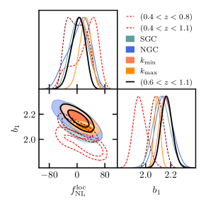
(a) Unblinded LRG (FKP) high-$z$.

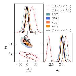
(b) Unblinded QSO (OQE).

Figure 21: Analogous of Figure 20 but using the unblinded data. The fiducial choices for our analysis, see Table 8, are displayed in black. The MAP values are given in Table 9. Note that the linear bias $b_{1}$ is higher with the unblinded data.

Table 9: Best-fit results with the unblinded LRGs and QSOs for different variations of our fiducial analysis. The central values are best fit values from the iminuit minimization while the errors are the 1$\sigma$ credible intervals from the chains. The window functions used during these fits contain both RIC and AIC contributions and were recomputed for the different configurations when it was needed. We use $k_{\rm min}=0.006~{}h\text{Mpc}^{-1}$ for the LRGs and $0.003~{}h\text{Mpc}^{-1}$ for the QSOs. The posteriors are displayed in Figure 21.

		$f_{\rm NL}^{\mathrm{loc}}$	$b_{1}$	$s_{n,0}$	$\Sigma_{s}$	$\chi_{\rm red}^{2}$
LRG (FKP)	high-$z$ fiducial	${6}_{-18}^{+22}$	${2.166}_{-0.045}^{+0.045}$	${-0.024}_{-0.075}^{+0.074}$	${3.70}_{-0.53}^{+0.68}$	1.24
$(0.6<z<1.1)$	NGC	${19}_{-25}^{+39}$	${2.132}_{-0.071}^{+0.062}$	${0.02}_{-0.100}^{+0.107}$	${3.84}_{-0.57}^{+0.96}$	0.93
	SGC	${4}_{-26}^{+25}$	${2.132}_{-0.069}^{+0.062}$	${0.05}_{-0.11}^{+0.11}$	${3.1}_{-0.90}^{+1.55}$	1.34
	$(0.4<z<0.8)$	${46}_{-19}^{+45}$	${1.936}_{-0.061}^{+0.044}$	${0.014}_{-0.088}^{+0.105}$	${3.14}_{-0.61}^{+1.23}$	0.62
	$(0.4<z<1.1)$	${-25}_{-34}^{+27}$	${2.124}_{-0.053}^{+0.047}$	${-0.101}_{-0.076}^{+0.081}$	${3.86}_{-0.42}^{+0.62}$	1.27
	$k_{\rm min}=0.008~{}h\text{Mpc}^{-1}$	${9}_{-22}^{+25}$	${2.161}_{-0.052}^{+0.045}$	${-0.017}_{-0.074}^{+0.084}$	${3.69}_{-0.54}^{+0.68}$	1.27
	$k_{\rm max}=0.1~{}h\text{Mpc}^{-1}$	${25}_{-15}^{+19}$	${2.092}_{-0.024}^{+0.024}$	${0.100}_{-0.029}^{+0.032}$	${2.65}_{-0.36}^{+0.53}$	1.24
QSO (OQE)	fiducial	${-2}_{-10.}^{+11}$	${3.048}_{-0.070}^{+0.064}$	${-0.039}_{-0.068}^{+0.076}$	${0.0}_{-1.41}^{+0.43}$	1.18
$(0.8<z<3.1)$	NGC	${2}_{-14}^{+14}$	${2.996}_{-0.082}^{+0.086}$	${-0.007}_{-0.086}^{+0.095}$	${0.0}_{-1.62}^{+0.49}$	1.19
	SGC	${-12}_{-18}^{+15}$	${3.09}_{-0.100}^{+0.123}$	${-0.02}_{-0.12}^{+0.12}$	${3.0}_{-1.7}^{+1.5}$	1.26
	$(0.8<z<2.1)$	${37}_{-18}^{+33}$	${2.353}_{-0.084}^{+0.067}$	${0.087}_{-0.079}^{+0.087}$	${0.0}_{-1.44}^{+0.43}$	0.61
	$(1.6<z<3.1)$	${-2.3}_{-8.4}^{+8.4}$	${3.236}_{-0.079}^{+0.088}$	${-0.055}_{-0.093}^{+0.090}$	${4.38}_{-0.88}^{+1.18}$	0.75
	$k_{\rm min}=0.008~{}h\text{Mpc}^{-1}$	${-5}_{-18}^{+14}$	${3.060}_{-0.080}^{+0.086}$	${-0.048}_{-0.085}^{+0.081}$	${0.7}_{-1.44}^{+0.45}$	1.22
	$k_{\rm max}=0.1~{}h\text{Mpc}^{-1}$	${3}_{-10.}^{+11}$	${2.987}_{-0.050}^{+0.048}$	${0.039}_{-0.041}^{+0.043}$	${2.17}_{-0.73}^{+1.20}$	1.14

The unblinded power spectrum for the LRG high-$z$ and the QSO (OQE), with their best fit that are given in Table 10 (first block), are displayed in Figure 22. The gray regions around the best fit model (black lines) are computed as the standard deviation of 1000 realizations of the theory generated with the posteriors from the chains partially shown in Figure 21 and centered around the best fit values given in Table 9. This region illustrates the $1\sigma$ fluctuation where the model can be, although in this case, each bin $k$ is not independent.

Hence, the choice of the analysis done in Section 5.3.3 remains viable, with the unblinded data requiring no further investigation.

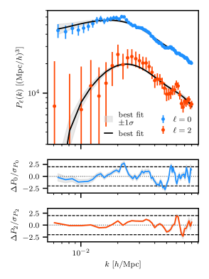
(a) LRG (FKP) high-$z$.

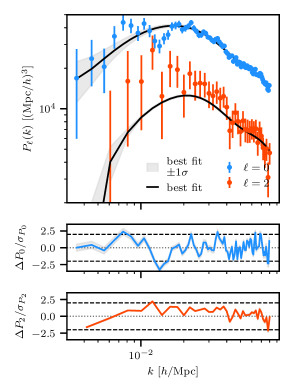
(b) QSO (OQE).

Figure 22: Monopole (blue) and quadrupole (red) of the unblinded DESI DR1 LRG high-$z$ (left) and QSO (right) with the best fit model (black). The errors are the standard deviation from the DR1 power-spectrum covariance matrix. The two lower panels give the relative difference normalised to the errors between the data and the best fit model. Gray regions around the best fit are the $1\sigma$ fluctuation of the model computed as the standard deviation of 1000 realizations of theory generated using the posteriors of the parameters.

6.2 Constraints on PNG with DESI DR1

The $f_{\rm NL}^{\rm loc}$ constraints from the LRG and QSO samples:

$$f_{\rm NL}^{\rm loc}={6}_{-18}^{+22}\quad(68\%)\quad\text{[LRG]}\quad\text{and}\quad f_{\rm NL}^{\rm loc}={-2}_{-10}^{+11}\quad(68\%)\quad\text{[QSO]}$$ (6.1)

are in good agreement such that one can combine them to improve the constraint on $f_{\rm NL}^{\rm loc}$. The best fit measurement and the posterior for the combination are shown in Table 10 (second block) and in Figure 23 in brown (resp. in purple) for LRG high-$z$ (FKP) + QSO (FKP) (resp. for LRG high-$z$ (FKP) + QSO(OQE)), as well as the summary of the independent measurements. Combining these two tracers leads to

$$f_{\rm NL}^{\rm loc}=-3.6_{-9.1}^{+9.0}\quad(68\%)\quad\left[\text{LRG}+\text{QSO}\right],$$ (6.2)

and improves the constraint by a factor of $10\%$ compared to QSO (OQE) alone. Moreover, we see that our combined results are compatible at the $<1\sigma$ level with $f_{\rm NL}^{\rm loc}$ measurement from CMB data by Planck in 2018 represented by the gray shaded region in Figure 23, given by $f_{\rm NL}^{\rm loc}=-0.9\pm 5.1$ at $68\%$ CL [7].

In this analysis, we have chosen a recent merger model for the QSO leading to $p=1.6$ since we do not have precise knowledge of $b_{\Phi}$, see [12, 51]. Adopting a more aggressive approach by setting $p=1.0$ leads to

$$f_{\rm NL}^{\rm loc}=1.7_{-7.7}^{+8.4}\quad(68\%)\quad\left[\text{LRG }(p=1.0)+\text{QSO }(p=1.0)\right]$$ (6.3)

when combining the LRG and the QSO sample, and reduces the $f_{\rm NL}^{\rm loc}$ error bars by a factor of $11\%$. The gain for QSO (OQE) alone is about $10\%$ compared to using $p=1.6$, as shown in the corresponding row of Table 10. For the case of $p=1.0$, we recomputed the power spectra with the OQE weights (Eq. 3.18), as well as the corresponding covariance matrix and the window matrix and its integral constraint contributions.

So far, we have built the bias model for $b_{\Phi}$ in our fitting procedure Eq. 2.6, linked to the linear bias $b_{1}$. Without further information about $b_{\Phi}$, one can only measure directly the product $b_{\Phi}\times f_{\rm NL}^{\rm loc}$ in Eq. 2.4, jointly with the linear bias $b_{1}$, which leads to

$$b_{\Phi}f_{\rm NL}^{\rm loc}={22}_{-63}^{+92}\quad(68\%)\quad\text{[LRG]}\quad\text{and}\quad b_{\Phi}f_{\rm NL}^{\rm loc}={-13}_{-56}^{+56}\quad(68\%)\quad\text{[QSO]}.$$ (6.4)

The constraints with DESI DR1 data are given in the last row of Table 10, but the uncertainties remain too large to provide meaningful insights in the search for PNGs. Note that as already shown with the EZmocks (see Table 4), the errors on the recovered parameters for the OQE weights are equal than the ones obtained with FKP weights, since in the case of the OQE weighting scheme the higher effective redshift leads to a higher value of $b_{\Phi}$, thus increasing the errors on the combined parameter $b_{\Phi}\times f_{\rm NL}^{\rm loc}$.

Since our combined constraints are compatible with $f_{\rm NL}^{\rm loc}=0$ at the $<1\sigma$ level, we can proceed to a sanity check by comparing the unblinded errors to the ones obtained with EZmocks, where $f_{\rm NL}^{\rm loc}=0$ was used (see Section 4.2). We note that the errors derived from the fit with the unblinded QSOs are remarkably in agreement with the ones given in Table 4 that we found during the fit of the mean on 1000 EZmocks. This comparison highlights that, at the scales over which we fit the data, our pipeline provides a fair description of the different statistical noises and accounts for the different systematic effects that appear in the real data. The LRG unblinded errors are larger than the EZmocks ones as expected, because we are considering here only the high-$z$ part of the sample. After re-normalising the EZmocks errors to the effective linear bias for the high-$z$ sample, the EZmocks and unblinded errors are compatible.

Table 10: Our final constraints on PNG, obtained with unblinded DR1 data. The central values are the best fit value from the iminuit minimization while the errors are the 1$\sigma$ credible interval from the chains. We use $k_{\rm min}=0.006~{}h\text{Mpc}^{-1}$ for the LRGs and $0.003~{}h\text{Mpc}^{-1}$ for the QSOs. The posteriors are displayed in Figure 23.

Individual ($f_{\rm NL}^{\rm loc}$)	$f_{\rm NL}^{\rm loc}$	$b_{1}$		$s_{n,0}$		$\Sigma_{s}$
LRG (FKP) high-$z$	${6}_{-18}^{+22}$	${2.166}_{-0.045}^{+0.045}$		${-0.024}_{-0.075}^{+0.074}$		${3.70}_{-0.53}^{+0.68}$
QSO (OQE)	${-2}_{-10.}^{+11}$	${3.048}_{-0.070}^{+0.064}$		${-0.039}_{-0.068}^{+0.076}$		${0.0}_{-1.41}^{+0.43}$
QSO (OQE) ($p=1.0$)	${3.5}_{-7.4}^{+10.7}$	${2.792}_{-0.064}^{+0.059}$		${-0.038}_{-0.067}^{+0.064}$		${1.8}_{-1.41}^{+0.74}$
Joint ($f_{\rm NL}^{\rm loc}$)	$f_{\rm NL}^{\rm loc}$	$b_{1}$		$s_{n,0}$		$\Sigma_{s}$
		LRG	QSO	LRG	QSO	LRG	QSO
LRG + QSO (OQE)	${-3.6}_{-9.1}^{+9.0}$	${2.181}_{-0.033}^{+0.035}$	${3.081}_{-0.070}^{+0.066}$	${-0.051}_{-0.062}^{+0.063}$	${-0.063}_{-0.078}^{+0.072}$	${3.64}_{-0.47}^{+0.67}$	${0.0}_{-1.36}^{+0.41}$
LRG + QSO (OQE) ($p=1.0$)	${1.7}_{-7.7}^{+8.4}$	${2.174}_{-0.032}^{+0.035}$	${2.816}_{-0.059}^{+0.065}$	${-0.042}_{-0.063}^{+0.063}$	${-0.054}_{-0.073}^{+0.063}$	${3.64}_{-0.52}^{+0.62}$	${1.6}_{-1.45}^{+0.60}$
Individual ($b_{\Phi}f_{\rm NL}^{\rm loc})$	$b_{\Phi}f_{\rm NL}^{\rm loc}$	$b_{1}$		$s_{n,0}$		$\Sigma_{s}$
LRG (FKP) high-$z$	${22}_{-63}^{+92}$	${2.166}_{-0.046}^{+0.045}$		${-0.024}_{-0.068}^{+0.082}$		${3.70}_{-0.49}^{+0.69}$
QSO (OQE)	${-13}_{-56}^{+56}$	${3.036}_{-0.066}^{+0.072}$		${-0.002}_{-0.072}^{+0.070}$		${2.7}_{-0.89}^{+1.36}$
QSO (OQE) ($p=1.0$)	${12}_{-47}^{+54}$	${2.800}_{-0.058}^{+0.058}$		${-0.039}_{-0.064}^{+0.058}$		${2.3}_{-1.0}^{+1.2}$

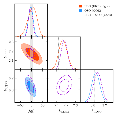
Figure 23: Posteriors in the $(b_{1},f_{\rm NL}^{\rm loc})$ plane of our final constraints on PNG, obtained with unblinded DR1 LRG and QSO samples. The gray band is the constraint from Planck 2018. The MAP values are given in Table 10. The gray dotted lines are the values of $b_{1}$ for LRG and QSO samples measured from the monopole of the 2-point correlation function, see Section A.1. We do not consider the cross-covariance between the LRGs and QSOs.

6.3 Evaluation of systematic errors

The errors presented in this analysis exclude any contribution from systematic errors. In this section, we provide an estimate of these errors. They are summed up in Table 11 where they are given as a percentage of the statistical error.

First, the geometrical description provided in Section 4.2 recovers the parameters of interest within $\sim 0.3\sigma$ in the worst case, see Table 4. Then, the systematic errors from the RIC contribution (Table 6) can be estimated by comparing the first and the last column of Table 6 and can lead up to $0.2\sigma$ discrepancy. Similarly, for the AIC contribution (Table 15), the systematic error is about $0.06\sigma$, see Table 6, so that one can neglect these systematics that come from our theoretical model. Note that in the case of the LRG, the systematic is estimated from the fit up to $k_{\rm min}=0.006h\text{Mpc}^{-1}$, while the systematics from our model is for $k_{\rm min}=0.003h\text{Mpc}^{-1}$, such that they should be even smaller for this new $k_{\rm min}$.

Regarding the efficiency of the imaging weights, we adopted conservative cuts to guard against any residual effects though it weakens our final constraints. With the upcoming data releases and the reduction of the statistical uncertainty on $f_{\rm NL}^{\rm loc}$, one will need to carefully assess the systematics in the future analysis. However, we can estimate it by looking the fluctuation in $f_{\rm NL}^{\rm loc}$ as a function of the different imaging weights in Table 16, the imaging systematics contribute to $0.22\sigma$ for the LRGs and $0.38\sigma$ for the QSOs. Hence, the imaging errors are still the most important source of the systematics in our analysis.

Finally, assuming all these contributions independent, one can add them in quadrature such that

$$\sigma_{\rm tot}=\sqrt{\sigma_{\rm stat}^{2}+\sigma_{\rm geo.}^{2}+\sigma_{\rm RIC}^{2}+\sigma_{\rm AIC}^{2}+\sigma_{w_{\rm sys}}^{2}}.$$ (6.5)

Hence, in the worst case (Table 11), the total systematic error represents an increase of $8\%$ for LRGs and $12\%$ for QSOs over the statistical errors alone. We neglect them in this analysis, and further work may be required as the data sample size increases with the next release of DESI data.

Table 11: Summary of the systematic error estimates in our analysis. All are given as a percentage of the associated statistical errors.

	LRG	QSO
Geometry	$34\%$	$26\%$
RIC	$6\%$	$20\%$
AIC	$6\%$	$6\%$
$w_{\rm sys}$	$22\%$	$38\%$

7 Conclusions

In this work, we investigate the large-scale modes of the power spectrum from the largest LRG and QSO sample from the first DESI data release. We then proceed to measure the scale-dependent bias with DESI the luminous red galaxies and quasars, and obtain the first constraints on the PNG parameter $f_{\rm NL}^{\rm loc}$ from DESI spectroscopic data.

We validate the power spectrum description that handles the geometrical effects used in DESI, and we develop an innovative method to include the radial integral constraint (RIC) and the angular integral constraint (AIC) contributions into the power spectrum window matrix formalism. RIC appears due to the use of the shuffling method that consists of drawing the randoms redshifts from the data ones, while AIC stems from the geometrical impact inherent to the regression method used to correct for imaging systematics. This is the first time that both of these two contributions are handled in a multiplicative way for the analysis of the large scale modes of the power spectrum. In addition, we show that using the optimal quadratic weights as in [14] improves our constraint on $f_{\rm NL}^{\rm loc}$ and does not bias the signal if the linear bias is sufficiently well constrained.

We re-weight the QSO and LRG angular distribution to mitigate the dependence of the target selection on the different imaging properties of the DESI Legacy Imaging Surveys. The bias introduced by these weights, along with the imaging systematics themselves, was the most important systematic effect in the previous measurement using large-scale structures [8, 17]. In this paper, our incorporation of the angular integral constraint (AIC) in the power spectrum window matrix enables us to not bias the measurement by using of standard imaging weights $w_{\rm sys}$. In addition, correctly handling this AIC contribution allows us to properly test the different imaging weights by looking at the impact of each weight on $f_{\rm NL}^{\rm loc}$.

Our $f_{\rm NL}^{\rm loc}$ measurement is carried out, for the first time, with a fully blinded procedure that enables us to make the fiducial choices of our analysis without any confirmation bias. Specifically, we decide to use the QSOs ($0.8<z<3.1$) with the optimal quadratic weights from $k_{\rm min}=0.003~{}h\text{Mpc}^{-1}$ to $k_{\rm max}=0.08~{}h\text{Mpc}^{-1}$, and the high-$z$ part of the LRG sample ($0.6<z<1.1$) with FKP weights from $k_{\rm min}=0.006~{}h\text{Mpc}^{-1}$ to $k_{\rm max}=0.08~{}h\text{Mpc}^{-1}$.

Combining both the DESI DR1 LRG and QSO samples, we find

$$f_{\rm NL}^{\rm loc}=\left\{\begin{array}[]{rl}-3.6_{-9.1}^{+9.0}&\quad(68\%)\quad\text{with }p_{\rm QSO}=1.6\\[4.30554pt] 1.7_{-7.7}^{+8.4}&\quad(68\%)\quad\text{with }p_{\rm QSO}=1.0\end{array}\right.$$ (7.1)

leading to the tightest constraint to date using the large-scale structure and improving by a factor $\sim 2.3$ the previous one performed with the latest data release of eBOSS: $-23<f_{\rm NL}^{\rm loc}<21$ [8, 14]. Our new measurement, despite the significant reduction in error bars, is in agreement with the one from Planck 2018: $f_{\rm NL}^{\rm loc}=-0.9\pm 5.1$ at $68\%$ confidence [7]. For each tracer independently, we obtain

$$f_{\rm NL}^{\rm loc}=\left\{\begin{array}[]{rl}6_{-18}^{+22}&\quad(68\%)\quad\text{LRG only}\\[4.30554pt] -2_{-10}^{+11}&\quad(68\%)\quad\text{QSO only with }p_{\rm QSO}=1.6\\[4.30554pt] 3.5_{-7.4}^{+10.7}&\quad(68\%)\quad\text{QSO only with }p_{\rm QSO}=1.0\end{array}\right..$$ (7.2)

This analysis could benefit from several improvements that we plan to implement in future analyses of DESI data. First, residual systematics in the LRG sample prevent us from using the full redshift sample and using larger scales up to $k_{\rm min}=0.003~{}h\text{Mpc}^{-1}$. The upcoming DESI DR2 data with a larger LRG sample should help us investigate these systematics and correct them. Furthermore, to better handle imaging systematics, we plan to enhance our imaging mitigation method and allow their redshift dependence within individual bins. Such improvements should be feasible in the future, in the forthcoming DESI data releases.

For the DESI Y5 data, we forecast that with our current maximal scale $k_{\rm min}=0.003~{}h\text{Mpc}^{-1}$ and by combining the full LRG and QSO samples, we should achieve $\sigma(f_{\rm NL}^{\rm loc})\sim 6.5$. Moreover, the geometrical model outlined here can be extended to larger scales, reaching $k_{\rm min}=0.001~{}h\text{Mpc}^{-1}$. We may need some additional validations for the window matrix computation and for the correct incorporation of the different integral constraint contributions into the window matrix. This larger maximal scale is expected to yield a 20–25$\%$ improvement in $f_{\rm NL}^{\rm loc}$ constraints, resulting in $\sigma(f_{\rm NL}^{\rm loc})\sim 5$. Thus, DESI data in the near future could approach the constraining power of the 2018 Planck CMB results [34].

Data Availability

Data from the plots in this paper will be available on Zenodo as part of DESI’s Data Management Plan. The data used in this analysis will be made public along with Data Release 1 of DESI planed in 2025.

Appendix A Appendices

A.1 Linear bias for DESI LRGs and QSOs

The optimal weighting scheme for measuring $f_{\rm NL}^{\rm loc}$, detailed in Section 3.2.2, assumes a redshift evolution of the linear bias $b_{1}$. Hence, we provide here the measurements of the linear bias of the LRGs and QSOs in several redshift bins from the unblind DESI DR1 data.

The linear bias is measured in the monopole of the 2-point correlation function $\xi_{0}$ using only the scales: $30\;h^{-1}\text{Mpc}<s<80\;h^{-1}\text{Mpc}$, so that one can only consider the simple Kaiser formula to take into account the redshift space distortion

$$\xi_{0}(s)=\left(b_{1}^{2}+\dfrac{2}{3}b_{1}f+\dfrac{1}{5}f^{2}\right)\xi_{\rm lin}(s),$$ (A.1)

where $f$ is the growth rate and $\xi_{\rm lin}$ is the linear 2-points correlation function obtained from Class. Both of these quantities are evaluated assuming Planck 2018 cosmology [34] and at an effective redshift that is computed as in Eq. 3.19. The covariance matrix that we use is estimated using the jackknife method with 128 sub-samples.

The linear bias for the LRGs and QSOs is given in Table 12, while these measurements are displayed in Figure 24. We propose a function to describe the redshift evolution and measure its parameters from the data; specifically,

$$b_{1}(z)=a(1+z)^{2}+b,$$ (A.2)

with $a,b=0.209\pm 0.025,1.415\pm 0.076$ for the DESI DR1 LRGs and $a,b=0.237\pm 0.010,0.771\pm 0.070$ for the DESI DR1 QSOs.

Table 12: Measurements of the linear bias $b_{1}$ of the LRGs and QSOs from the unblind DESI DR1 data.

Tracer	$z_{\rm min}$ – $z_{\rm max}$	$z_{\rm eff}$	$b_{1}$
LRG	0.4 – 0.5	0.45	$1.834\pm 0.036$
	0.5 – 0.6	0.55	$1.900\pm 0.038$
	0.6 – 0.7	0.65	$2.029\pm 0.037$
	0.7 – 08	0.75	$2.053\pm 0.033$
	0.8 – 0.9	0.84	$2.153\pm 0.038$
	0.9 – 1.0	0.94	$2.217\pm 0.040$
	1.0 – 1.1	1.03	$2.167\pm 0.069$
QSO	0.8 – 1.0	0.90	$1.579\pm 0.057$
	1.0 – 1.2	1.10	$1.851\pm 0.067$
	1.2 – 1.4	1.29	$2.116\pm 0.062$
	1.4 – 1.6	1.49	$2.263\pm 0.064$
	1.6 – 1.8	1.69	$2.355\pm 0.084$
	1.8 – 2.0	1.89	$2.713\pm 0.078$
	2.0 – 2.2	2.09	$3.070\pm 0.097$
	2.2 – 2.6	2.36	$3.551\pm 0.098$
	2.6 – 3.0	2.76	$4.137\pm 0.156$
	3.0 – 3.5	3.15	$4.350\pm 0.418$

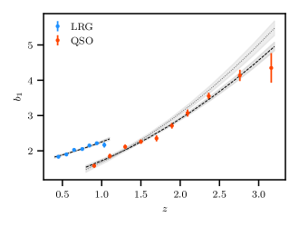
Figure 24: Redshift evolution of the linear bias $b_{1}$ as measured in the unblind DESI DR1 LRGs (blue) and QSOs (red). Black dashed lines are the best fit of Eq. A.2 to these points, while the gray dotted line is the redshift evolution measured from the BOSS and eBOSS QSO sample [117]. Gray regions around the best fit are the 1$\sigma$ fluctuation of the model computed as the standard deviation of 1000 theory generated assuming Gaussian posteriors of the parameters with covariance matrix from the best fit.

Note that we can transform Eq. A.2 to match the function used in [117]:

$$b_{1}(z)=a_{L}\left[(1+z)^{2}-6.565\right]+b_{L},$$ (A.3)

where $a_{L},b_{L}=0.237\pm 0.010,2.328\pm 0.026$ for the DESI DR1 QSOs. For comparison, [117] found for the BOSS/eBOSS QSO sample a slightly higher bias at high redshift described by $a_{L},b_{L}=0.278\pm 0.018,2.393\pm 0.042$.

A.2 Impact of imaging systematic weights

Despite the low stellar and extra-galactic contamination of the DESI galaxy clustering sample thanks to the spectroscopy, the fluctuations imprinted into the target density still play a major role at the large scales of the power spectrum.

Figure 25 shows the monopole for the different dark time tracers of DESI, namely the Luminous Red Galaxies (LRG) with 0.4 < z < 1.1 [53], Emission Line Galaxies (ELG) with 0.8 < z < 1.6 [66] and the Quasars (QSO) with 0.8 < z < 3.1 [54], with and without the imaging systematic weights that mitigate these spurious fluctuations.

The value of $f_{\rm NL}^{\rm loc}$ measured without applying the imaging systematic weights for LRGs and QSOs was given in Table 16. Recall that, due to a residual systematic, which we are not able to correct in the LRG sample, we had to increased $k_{\rm min}$ from $0.003$ to $0.006~{}h\text{Mpc}^{-1}$ such that the imaging systematic weights have no impact on the monopole and on the $f_{\rm NL}^{\rm loc}$ measurement.

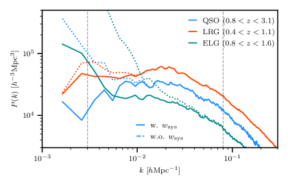
Figure 25: Monopoles of the DESI DR1 LRG, ELG, and QSO samples with the blinding scheme applied. Solid lines are with the imaging systematic weights, while the dotted ones are without.

A.3 Impact of photometric region normalization on the power spectrum

As described in Section 3.2.4, one need to normalize South (NGC) to North when we compute the power spectrum on all the NGC as well as South (SGC) to the DES region for the full SGC part of the footprint. The normalization means that $\alpha$ in Eq. 3.5 is set to match the corresponding data separately in each region.

In particular, one needs to perform this renormalization between the South (SGC) and DES even though the two regions are from the same photometric survey. Figure 26 shows the monopole for the blinded QSO sample without the normalization factor (yellow) that exhibits an excess of power at large scales compared with the monopole computed to the normalization factor given in Eq. 3.20 (green). Not accounting for this normalization would bias the measurement of primordial non-Gaussianity.

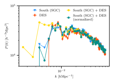
Figure 26: Comparison of the monopole of the blinded QSO sample computed either on South (SGC) (blue), DES (red), South (SGC) + DES without the normalization (yellow) or with the normalization given in Eq. 3.20 (green).

A.4 Impact of quadrupole on PNG measurement

Table 13 shows the gain of including the quadrupole ($\ell=2$) during the fit. It leads only to few percent of improvement and can be neglected in this entire analysis, simplifying a lot the measurement with the OQE weights. However, for completeness, we include it during all the analysis.

Table 13: Result of the fit using the mean of the power spectrum over 1000 realizations including or not the quadrupole ($\ell=2$) with the corresponding covariance matrix for the LRGs and QSOs. Central values and the errors are both from the MCMC chains.

	with $\ell=2$		without $\ell=2$
	$f_{\rm NL}^{\rm loc}$	$b_{1}$	$f_{\rm NL}^{\rm loc}$	$b_{1}$
LRG Y1 (FKP)	${5}_{-11}^{+18}$	${2.065}_{-0.037}^{+0.032}$	${7}_{-12}^{+18}$	${2.032}_{-0.044}^{+0.043}$
LRG Y5 (FKP)	${3.8}_{-7.5}^{+10.7}$	${2.065}_{-0.024}^{+0.021}$	${2.5}_{-8.9}^{+9.8}$	${2.044}_{-0.044}^{+0.043}$
QSO Y1 (FKP)	${3.0}_{-13}^{+18}$	${2.440}_{-0.046}^{+0.050}$	${2}_{-14}^{+18}$	${2.427}_{-0.069}^{+0.060}$
QSO Y5 (FKP)	${4.6}_{-9.6}^{+9.9}$	${2.435}_{-0.033}^{+0.030}$	${3}_{-10.0}^{+10.3}$	${2.417}_{-0.051}^{+0.050}$
QSO Y1 (OQE)	${-4}_{-10}^{+13}$	${3.088}_{-0.080}^{+0.064}$	${1}_{-10}^{+13}$	${3.009}_{-0.088}^{+0.080}$
QSO Y5 (OQE)	${-1.4}_{-7.8}^{+7.8}$	${3.083}_{-0.049}^{+0.045}$	${1.8}_{-7.4}^{+8.7}$	${2.994}_{-0.062}^{+0.071}$

A.5 Global Integral Constraint

As explained in [118, 119, 120, 121, 95], the real mean density of the tracer in the Universe, used in the FKP field (Eq. 3.5), is unknown and has to be estimated from our finite survey volume. Such an estimation suppresses all the fluctuations with scales larger than the survey size such $P(k)\underset{k\to 0}{\longrightarrow}0$. This effect is known as the global integral constraint (GIC) and can be taken into account in the convolved prediction (Eq. 4.8):

$$\left(P_{\ell}^{\rm obs}\right)_{i}=\left(\mathcal{W}_{\ell\ell^{\prime}}\right)_{ij}\left(P_{\ell^{\prime}}\right)_{j}-\left(\mathcal{W}^{\mathrm{GIC}}_{\ell\ell^{\prime}}\right)_{ij}\left(P_{\ell\prime}^{\mathrm{theo}}\right)_{j},$$ (A.4)

where the summation runs over $\ell^{\prime}$ and $j$. The contribution of the global integral constraint $\left(\mathcal{W}^{\mathrm{GIC}}_{\ell\ell^{\prime}}\right)_{ij}$ is given by

$$\left(\mathcal{W}^{\mathrm{GIC}}_{\ell\ell^{\prime}}\right)_{ij}=\left(\mathcal{W}_{\ell 0}\right)_{i0}/\left(\mathcal{W}_{00}\right)_{00}\left(\mathcal{W}_{0\ell^{\prime}}\right)_{0j}.$$ (A.5)

The GIC contribution in Eq. A.4 is directly proportional to $P_{\ell=0}(k\rightarrow 0)$ [95] such that this contribution depends on the value of $f_{\rm NL}^{\rm loc}$ used to evaluate the theory. The convolved power spectrum for LRGs and QSOs at very large scales ($k<10^{-3}~{}[h/\mathrm{Mpc}]$) is displayed Figure 27. The convolved monopole of the power spectrum converges at very large scales to a non-zero value such that the contribution of the GIC is 4 (resp. 10) times larger for a situation with $f_{\rm NL}^{\rm loc}=20$ compared to $f_{\rm NL}^{\rm loc}=0$.

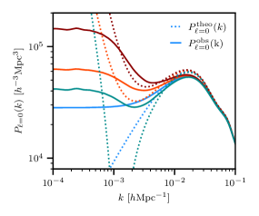
(a) LRG ($0.4<z<1.1$) with FKP.

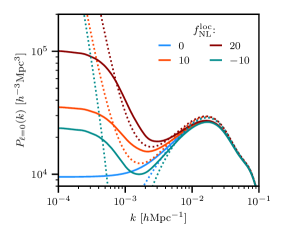
(b) QSO ($0.8<z<3.1$) with FKP.

Figure 27: Monopole of the power spectrum for LRGs (left) and QSOs (right) for several values of $f_{\rm NL}^{\rm loc}$ at very large-scales. The convolved (resp. unconvolved) monopole is shown in solid (resp. dashed) lines. The value of $P_{\ell=0}(k\rightarrow 0)$ depends of $f_{\rm NL}^{\rm loc}$.

The GIC contribution is shown in Figure 28 for the DESI DR1 sample. As expected, the GIC contribution is larger for the LRGs since they probe a smaller volume of the Universe than the QSOs. In the QSO case, the GIC contribution, even for an underlying value of $f_{\rm NL}^{\rm loc}=20$ is negligible compared to the fluctuation of the signal due to a modification of $\Delta f_{\rm NL}^{\rm loc}=1$ for the scales of interest ($k>0.003~{}[h/\mathrm{Mpc}]$). For the LRGs, the contribution becomes comparable to the fluctuation of the signal due to a modification of $\Delta f_{\rm NL}^{\rm loc}=1$ for the largest scales. As shown in the following, the expected sensitivity for $f_{\rm NL}^{\rm loc}$ with this sample is about $14.5$ so that one can neglect this impact, especially because this contribution impacts only the largest scales that are the one with the most statistical uncertainty, see (Figure 4). Since these scales are also very sensitive to the residual imaging systematics, such that one need for the data to increase our fiducial value (see the following section, Section 4.2) of $k_{\rm min}$ to $0.006~{}[h/\mathrm{Mpc}]$ where the contribution becomes, as for the QSOs, negligible compare the fluctuation of the signal for $\Delta f_{\rm NL}^{\rm loc}=1$.

Since, this contribution does not contribute significantly to our measurement, we do not include its contribution to the window matrix $\mathcal{W}$. Note that this contribution is lower due to the increase of the survey size of the upcoming DESI data release, such that one can certainly still neglect it even in light of the reduction in errors associated with this new data.

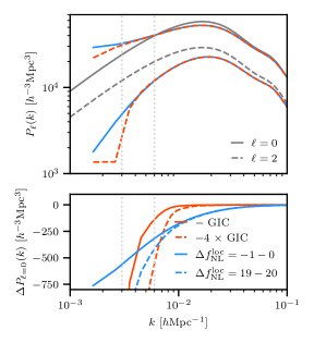
(a) LRG ($0.4<z<1.1$) with FKP.

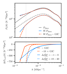
(b) QSO ($0.8<z<3.1$) with FKP.

Figure 28: Top panel: Convolved power spectrum with the global integral constraint contribution (red dashed lines) on the monopole and the quadrupole for the LRGs (left) and the QSOs (right) compared to the convolved power spectrum given by Eq. 4.8 (blue lines). The gray lines are the unconvolved monopoles. Bottom panel: Comparison between the GIC contribution for $f_{\rm NL}^{\rm loc}=0$ (resp. $f_{\rm NL}^{\rm loc}=20$) in red solid (resp. dashed) lines and the amplitude of the signal of $\Delta f_{\rm NL}^{\rm loc}=-1$ at $f_{\rm NL}^{\rm loc}=0$ (resp. $f_{\rm NL}^{\rm loc}=20$) in solid (resp. dashed) blue lines.

A.6 Target selection dependence on the PSF detection at low-z.

As noted in [54] (Fig. 11), the QSO target selection requires objects to be classified as point sources, which leads to the exclusion of many low-redshift quasars classified as extended sources as their host galaxies were resolved. Improved photometry exacerbates this issue, as more host galaxies are resolved, meaning the number of low-redshift quasars affected more so than the number of their higher-redshift counterparts. This behavior is demonstrated in Figure 29, where the low-redshift sample ($0.8<z<1.3$) in red shows a distinct pattern compared to the mid-redshift sample ($1.3<z<2.1$) in green. The choice $z=1.3$ is motivated by comparing the relative density as a function of the PSF Depth $z$ of several redshift bins.

The figure highlights the dependence on PSF depth in the z-band, the deepest band in the Legacy Surveys which drives object morphology classification. The distinct behavior of the low-redshift sample is masked when analysing the full range ($0.8<z<2.1$) and cannot be properly addressed with imaging systematic weights computed across the entire sample. However, the small fraction of low-redshift objects ($23\%$ of the data) has a significant impact on the large-scale modes of the power spectrum if not properly accounted for.

Figure 30 compares the monopole across different photometric regions: using a single weight for the full sample (solid markers) versus separate weights (open markers) for the two redshift ranges, 0.8 < z < 1.3 and 1.3 < z < 2.1. Without these tailored weights, it becomes impossible to correctly measure the large-scale modes of the power spectrum.

We note that this improvement in imaging systematic weights does not yet account for any redshift dependence within the sub-samples. Addressing this limitation is left to future work, expected with the next DESI data release.

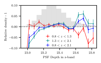
Figure 29: Relative density of the QSO sample for different redshift subsamples as a function of PSF Depth $z$ in the South (NGC+SGC) region. The histogram represents the fraction of objects in each bin of the observational feature and the error bars are the estimated standard deviation of the normalized density in each bin.

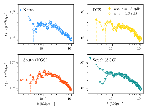
Figure 30: Comparison of the monopole of the blinded QSO sample with (empty marker) or without (solid marker) the additional split at $z=1.3$ to compute the imaging systematic weights.

A.7 Additional tables

In this appendix, we include several tables that were used to generate figures in the main text and that we may need for the assessment of systematic errors.

Table 14: Best fit results on the mocks for the LRGs and QSOs (mean over 10 realizations) using either FKP and OQE weights, for various configurations of imaging weights with the radial integral constraint but without the angular integral constraint. The errors are from the minimization performed with iminuit. The $f_{\rm NL}^{\rm loc}$ values are plotted in Figure 15 for visualization.

		$f_{\rm NL}^{\mathrm{loc}}$	$b_{1}$	$s_{n,0}$	$\Sigma_{s}$
LRG (FKP)	No weight	$4\pm 13$	$2.066\pm 0.032$	$0.044\pm 0.061$	$4.32\pm 0.44$
$k_{\rm min}=0.003~{}h\text{Mpc}^{-1}$	Default (RF 128)	$-24\pm 17$	$2.102\pm 0.038$	$0.009\pm 0.068$	$4.58\pm 0.41$
	Default (RF 256)	$-22\pm 14$	$2.103\pm 0.036$	$0.003\pm 0.065$	$4.61\pm 0.41$
	Default (Linear 256)	$1\pm 16$	$2.068\pm 0.035$	$0.044\pm 0.063$	$4.31\pm 0.44$
	PSF Depth (Linear 256)	$1\pm 16$	$2.068\pm 0.034$	$0.045\pm 0.063$	$4.31\pm 0.44$
	Same Feature Zbin (Linear 128)	$-5\pm 19$	$2.075\pm 0.038$	$0.038\pm 0.067$	$4.31\pm 0.44$
	Same Feature Zbin (Linear 256)	$-6\pm 18$	$2.076\pm 0.037$	$0.035\pm 0.066$	$4.33\pm 0.44$
	With DES (Linear 256)	$0.\pm 16$	$2.069\pm 0.035$	$0.044\pm 0.063$	$4.31\pm 0.44$
	4 regions (Linear 256)	$-4\pm 18$	$2.074\pm 0.037$	$0.038\pm 0.066$	$4.32\pm 0.44$
LRG (FKP)	No weight	$7\pm 18$	$2.062\pm 0.038$	$0.049\pm 0.067$	$4.31\pm 0.44$
$k_{\rm min}=0.006~{}h\text{Mpc}^{-1}$	Default (RF 128)	$-19\pm 20$	$2.096\pm 0.040$	$0.016\pm 0.070$	$4.57\pm 0.42$
	Default (RF 256)	$-23\pm 20$	$2.104\pm 0.041$	$0.001\pm 0.070$	$4.60\pm 0.41$
	Default (Linear 256)	$1\pm 19$	$2.070\pm 0.039$	$0.042\pm 0.068$	$4.32\pm 0.44$
	PSF Depth (Linear 256)	$1\pm 19$	$2.070\pm 0.039$	$0.042\pm 0.068$	$4.32\pm 0.44$
	Same Feature Zbin (Linear 128)	$-4\pm 19$	$2.075\pm 0.039$	$0.037\pm 0.069$	$4.32\pm 0.44$
	Same Feature Zbin (Linear 256)	$-5\pm 20.$	$2.076\pm 0.039$	$0.036\pm 0.069$	$4.33\pm 0.44$
	With DES (Linear 256)	$1\pm 19$	$2.069\pm 0.039$	$0.042\pm 0.068$	$4.32\pm 0.44$
	4 regions (Linear 256)	$-2\pm 19$	$2.073\pm 0.039$	$0.039\pm 0.068$	$4.33\pm 0.44$
QSO (FKP)	No weight	$6\pm 16$	$2.428\pm 0.047$	$0.007\pm 0.053$	$2.71\pm 0.87$
	Default (RF 256)	$-16\pm 15$	$2.467\pm 0.048$	$-0.017\pm 0.053$	$3.19\pm 0.74$
	No PSF Depth (RF 128)	$5\pm 15$	$2.431\pm 0.046$	$-0.001\pm 0.052$	$3.20\pm 0.75$
	Default (Linear 128)	$0\pm 17$	$2.439\pm 0.049$	$0.000\pm 0.054$	$2.75\pm 0.85$
	Default (Linear 256)	$-3\pm 17$	$2.445\pm 0.050$	$-0.004\pm 0.054$	$2.74\pm 0.86$
	No PSF Size (Linear 128)	$1\pm 17$	$2.437\pm 0.049$	$0.001\pm 0.053$	$2.75\pm 0.85$
QSO (OQE)	No weight	$0\pm 12$	$3.062\pm 0.071$	$-0.020\pm 0.074$	$0.0\pm 9.2$
	Default (RF 256)	$-10\pm 11$	$3.101\pm 0.069$	$-0.054\pm 0.073$	$0.0\pm 7.9$
	No PSF Depth (RF 128)	$4.0\pm 9.9$	$3.050\pm 0.066$	$-0.029\pm 0.070$	$0.0\pm 6.9$
	Default (Linear 128)	$-3\pm 13$	$3.071\pm 0.075$	$-0.027\pm 0.077$	$0.0\pm 6.3$
	Default (Linear 256)	$-6\pm 14$	$3.085\pm 0.079$	$-0.035\pm 0.079$	$0.0\pm 5.2$
	No PSF Size (Linear 128)	$-2\pm 13$	$3.070\pm 0.074$	$-0.026\pm 0.076$	$0.0\pm 9.1$

Table 15: Result of the fit on the mocks using the DR1 covariance matrix on the mean of the power spectrum with FKP weights over 30 realizations for the LRGs and QSOs without (first column) / with (second column) the imaging systematic weights and adding the angular integral constraint contribution into the window function (third column). The central values and errors are from the minuit minimization. The first column is comparable to the result from Table 4. These values are sum up in Figure 16

	params	w.o. $w_{sys}$	w. $w_{sys}$	w. $w_{sys}$ + AIC
DR1 LRG (FKP)	$f_{\rm NL}^{\rm loc}$	$4\pm 13$	$-24\pm 17$	$-1\pm 19$
Default	$b_{1}$	$2.067\pm 0.032$	$2.102\pm 0.038$	$2.074\pm 0.037$
(RF 256)	$s_{n,0}$	$0.042\pm 0.061$	$0.009\pm 0.068$	$0.026\pm 0.065$
	$\Sigma_{s}$	$4.32\pm 0.44$	$4.58\pm 0.41$	$4.50\pm 0.43$
Default	$f_{\rm NL}^{\rm loc}$	$4\pm 13$	$0.\pm 16$	$3\pm 14$
(Linear 256)	$b_{1}$	$2.067\pm 0.032$	$2.070\pm 0.035$	$2.066\pm 0.033$
	$s_{n,0}$	$0.042\pm 0.061$	$0.042\pm 0.063$	$0.044\pm 0.062$
	$\Sigma_{s}$	$4.32\pm 0.44$	$4.30\pm 0.44$	$4.31\pm 0.44$
Same Feature Zbin	$f_{\rm NL}^{\rm loc}$	$4\pm 13$	$-6\pm 19$	$3\pm 15$
(Linear 256)	$b_{1}$	$2.067\pm 0.032$	$2.076\pm 0.038$	$2.065\pm 0.033$
	$s_{n,0}$	$0.042\pm 0.061$	$0.035\pm 0.067$	$0.047\pm 0.062$
	$\Sigma_{s}$	$4.32\pm 0.44$	$4.31\pm 0.44$	$4.33\pm 0.44$
DR1 QSO (FKP)	$f_{\rm NL}^{\rm loc}$	$6\pm 16$	$-16\pm 15$	$4\pm 16$
Default	$b_{1}$	$2.428\pm 0.047$	$2.467\pm 0.048$	$2.428\pm 0.048$
(RF 256)	$s_{n,0}$	$0.007\pm 0.053$	$-0.017\pm 0.053$	$0.013\pm 0.053$
	$\Sigma_{s}$	$2.71\pm 0.87$	$3.19\pm 0.74$	$2.91\pm 0.81$
Default	$f_{\rm NL}^{\rm loc}$	$6\pm 16$	$0.\pm 17$	$5\pm 16$
(Linear 128)	$b_{1}$	$2.428\pm 0.047$	$2.439\pm 0.049$	$2.434\pm 0.048$
	$s_{n,0}$	$0.007\pm 0.053$	$0.000\pm 0.054$	$-0.003\pm 0.053$
	$\Sigma_{s}$	$2.71\pm 0.87$	$2.75\pm 0.85$	$2.42\pm 0.94$
Default	$f_{\rm NL}^{\rm loc}$	$6\pm 16$	$-3\pm 17$	$4\pm 17$
(Linear 256)	$b_{1}$	$2.428\pm 0.047$	$2.445\pm 0.050$	$2.433\pm 0.049$
	$s_{n,0}$	$0.007\pm 0.053$	$-0.004\pm 0.054$	$0.001\pm 0.053$
	$\Sigma_{s}$	$2.71\pm 0.87$	$2.74\pm 0.86$	$2.55\pm 0.90$

Table 16: Values used for Figure 19. Best fit results for the DR1 blinded LRGs and blinded QSOs using either FKP ot OQE weights, for various configurations of imaging weights. All the fits include the radial and angular integral constraint contributions. The errors and the central values are from the minimization performed with iminuit and the covariance matrix is the one from the 1000 EZmocks. The green rows are the default choices for the analysis on the unblinded data.

	features (method)	$f_{\rm NL}^{\mathrm{loc}}$	$b_{1}$	$s_{n,0}$	$\Sigma_{s}$
LRG (FKP)	No imaging weights	$42.6\pm 6.9$	$2.018\pm 0.028$	$0.125\pm 0.056$	$4.50\pm 0.43$
$k_{\rm min}=0.003~{}h\text{Mpc}^{-1}$	Default (RF 128)	$16\pm 10.$	$2.069\pm 0.029$	$0.036\pm 0.058$	$4.53\pm 0.41$
	Default (RF 256)	$22.5\pm 9.0$	$2.061\pm 0.029$	$0.059\pm 0.058$	$4.81\pm 0.40$
	Default (Linear 256)	$24.2\pm 9.3$	$2.041\pm 0.029$	$0.089\pm 0.057$	$4.52\pm 0.42$
	PSF Depth (Linear 256)	$25.1\pm 9.1$	$2.041\pm 0.029$	$0.090\pm 0.057$	$4.52\pm 0.42$
	Same Feature Zbin (Linear 128)	$20.\pm 10.$	$2.044\pm 0.030$	$0.086\pm 0.058$	$4.56\pm 0.42$
	Same Feature Zbin (Linear 256)	$25.4\pm 9.3$	$2.042\pm 0.029$	$0.088\pm 0.057$	$4.56\pm 0.42$
	With DES (Linear 256)	$26.5\pm 8.9$	$2.039\pm 0.029$	$0.097\pm 0.057$	$4.61\pm 0.42$
	4 regions (Linear 256)	$25.5\pm 9.3$	$2.039\pm 0.029$	$0.092\pm 0.057$	$4.53\pm 0.42$
LRG (FKP)	No imaging weights	$28\pm 15$	$2.041\pm 0.033$	$0.090\pm 0.061$	$4.57\pm 0.42$
$k_{\rm min}=0.006~{}h\text{Mpc}^{-1}$	Default (RF 128)	$27\pm 16$	$2.059\pm 0.032$	$0.046\pm 0.060$	$4.48\pm 0.42$
	Default (RF 256)	$28\pm 14$	$2.059\pm 0.031$	$0.061\pm 0.060$	$4.82\pm 0.40$
	Default (Linear 256)	$24\pm 18$	$2.044\pm 0.035$	$0.086\pm 0.063$	$4.54\pm 0.42$
	PSF Depth (Linear 256)	$25\pm 17$	$2.043\pm 0.035$	$0.087\pm 0.063$	$4.54\pm 0.42$
	Same Feature Zbin (Linear 128)	$20.\pm 18$	$2.048\pm 0.035$	$0.081\pm 0.063$	$4.58\pm 0.42$
	Same Feature Zbin (Linear 256)	$28\pm 17$	$2.041\pm 0.034$	$0.089\pm 0.062$	$4.57\pm 0.42$
	With DES (Linear 256)	$37\pm 15$	$2.029\pm 0.032$	$0.108\pm 0.060$	$4.60\pm 0.42$
	4 regions (Linear 256)	$26\pm 18$	$2.041\pm 0.034$	$0.090\pm 0.062$	$4.55\pm 0.42$
QSO (FKP)	No imaging weights	$140.\pm 17$	$2.109\pm 0.039$	$0.274\pm 0.044$	$7.61\pm 0.50$
$k_{\rm min}=0.003~{}h\text{Mpc}^{-1}$	Default (RF 256)	$35\pm 19$	$2.218\pm 0.044$	$0.213\pm 0.049$	$7.58\pm 0.47$
	no PSF Depth (RF 128)	$64\pm 21$	$2.203\pm 0.042$	$0.204\pm 0.046$	$7.42\pm 0.48$
	Default (Linear 256)	$31\pm 21$	$2.206\pm 0.046$	$0.204\pm 0.049$	$7.37\pm 0.48$
	Default (Linear 128)	$28\pm 22$	$2.210\pm 0.048$	$0.196\pm 0.050$	$7.23\pm 0.48$
	no PSF Size (Linear 128)	$34\pm 22$	$2.203\pm 0.047$	$0.208\pm 0.050$	$7.35\pm 0.48$
QSO (OQE)	No imaging weights	$39\pm 11$	$2.689\pm 0.061$	$0.241\pm 0.063$	$7.50\pm 0.63$
$k_{\rm min}=0.003~{}h\text{Mpc}^{-1}$	Default (RF 256)	$7\pm 18$	$2.790\pm 0.078$	$0.169\pm 0.073$	$7.68\pm 0.60$
	no PSF Depth (RF 128)	$-1\pm 13$	$2.782\pm 0.069$	$0.190\pm 0.069$	$7.77\pm 0.61$
	Default (Linear 256)	$-4\pm 14$	$2.799\pm 0.073$	$0.171\pm 0.071$	$7.85\pm 0.60$
	Default (Linear 128)	$-9\pm 15$	$2.822\pm 0.075$	$0.147\pm 0.072$	$7.62\pm 0.60$
	no PSF Size (Linear 128)	$-10.\pm 14$	$2.824\pm 0.074$	$0.148\pm 0.071$	$7.67\pm 0.60$

Table 17: Best-fit results from the blinded LRGs and QSOs for different variations of our fiducial analysis. The central values are best fit value from the iminuit minimization while the errors are the 1$\sigma$ credible intervals from the chains. The window functions used during these fits contain both RIC and AIC contributions and were recomputed for the different configurations when it was needed. We use $k_{\rm min}=0.006~{}h\text{Mpc}^{-1}$ for the LRGs and $0.003~{}h\text{Mpc}^{-1}$ for the QSOs. The posteriors are displayed in Figure 20.

		$f_{\rm NL}^{\mathrm{loc}}$	$b_{1}$	$s_{n,0}$	$\Sigma_{s}$
LRG (FKP)	fiducial	${24}_{-15}^{+19}$	${2.044}_{-0.039}^{+0.032}$	${0.086}_{-0.063}^{+0.066}$	${4.54}_{-0.42}^{+0.44}$
$(0.4<z<1.1)$	NGC	${27}_{-16}^{+25}$	${2.062}_{-0.046}^{+0.043}$	${0.054}_{-0.082}^{+0.080}$	${4.86}_{-0.48}^{+0.57}$
	SGC	${-7}_{-26}^{+25}$	${2.051}_{-0.057}^{+0.057}$	${0.08}_{-0.11}^{+0.10}$	${3.81}_{-0.67}^{+1.13}$
	$(0.4<z<0.8)$	${16}_{-28}^{+33}$	${1.993}_{-0.051}^{+0.050}$	${-0.01}_{-0.087}^{+0.106}$	${3.63}_{-0.52}^{+1.00}$
	$(0.6<z<1.1)$	${22}_{-17}^{+20}$	${2.137}_{-0.044}^{+0.041}$	${0.081}_{-0.068}^{+0.076}$	${4.72}_{-0.45}^{+0.51}$
	$k_{\rm min}=0.008~{}h\text{Mpc}^{-1}$	${64}_{-19}^{+33}$	${1.994}_{-0.043}^{+0.038}$	${0.153}_{-0.061}^{+0.076}$	${4.47}_{-0.43}^{+0.44}$
	$k_{\rm max}=0.1~{}h\text{Mpc}^{-1}$	${34}_{-13}^{+16}$	${2.017}_{-0.020}^{+0.019}$	${0.100}_{-0.026}^{+0.029}$	${3.38}_{-0.30}^{+0.31}$
LRG (FKP)	NGC	${32}_{-19}^{+31}$	${2.133}_{-0.067}^{+0.053}$	$0.084_{-0.092}^{+0.107}$	${4.95}_{-0.54}^{+0.62}$
$(0.6<z<1.1)$	SGC	${2}_{-30.}^{+27}$	${2.128}_{-0.064}^{+0.074}$	${0.10}_{-0.13}^{+0.10}$	${4.08}_{-0.77}^{+1.19}$
	$k_{\rm min}=0.008~{}h\text{Mpc}^{-1}$	${41}_{-24}^{+25}$	${2.109}_{-0.046}^{+0.047}$	${0.117}_{-0.079}^{+0.072}$	${4.65}_{-0.44}^{+0.56}$
	$k_{\rm max}=0.1~{}h\text{Mpc}^{-1}$	${37}_{-15}^{+16}$	${2.096}_{-0.025}^{+0.022}$	${0.107}_{-0.029}^{+0.031}$	${2.94}_{-0.36}^{+0.43}$
QSO (FKP)	fiducial	${28}_{-22}^{+23}$	${2.210}_{-0.054}^{+0.044}$	${0.197}_{-0.050}^{+0.050}$	${7.23}_{-0.47}^{+0.51}$
$(0.8<z<3.1)$	NGC	${47}_{-21}^{+33}$	${2.199}_{-0.059}^{+0.062}$	${0.212}_{-0.061}^{+0.063}$	${7.11}_{-0.65}^{+0.67}$
	SGC	${12}_{-40}^{+36}$	${2.247}_{-0.086}^{+0.084}$	${0.183}_{-0.077}^{+0.095}$	${7.23}_{-0.68}^{+0.79}$
	$(0.8<z<2.1)$	${101}_{-55}^{+53}$	${1.905}_{-0.055}^{+0.047}$	${0.276}_{-0.054}^{+0.055}$	${6.90}_{-0.59}^{+0.67}$
	$(1.6<z<3.1)$	${-22}_{-22}^{+15}$	${2.783}_{-0.082}^{+0.083}$	${0.178}_{-0.067}^{+0.079}$	${9.16}_{-0.43}^{+0.72}$
	$k_{\rm min}=0.008~{}h\text{Mpc}^{-1}$	${44}_{-43}^{+42}$	${2.195}_{-0.066}^{+0.059}$	${0.206}_{-0.053}^{+0.060}$	${7.20}_{-0.49}^{+0.51}$
	$k_{\rm max}=0.1~{}h\text{Mpc}^{-1}$	${32}_{-16}^{+23}$	${2.225}_{-0.033}^{+0.034}$	${0.144}_{-0.029}^{+0.030}$	${6.20}_{-0.37}^{+0.36}$
QSO (OQE)	fiducial	${-9}_{-15}^{+13}$	${2.822}_{-0.083}^{+0.064}$	${0.147}_{-0.069}^{+0.073}$	${7.62}_{-0.58}^{+0.64}$
$(0.8<z<3.1)$	NGC	${-8}_{-18}^{+18}$	${2.783}_{-0.088}^{+0.094}$	${0.164}_{-0.092}^{+0.085}$	${7.34}_{-0.77}^{+0.84}$
	SGC	${-11}_{-23}^{+20}$	${2.84}_{-0.11}^{+0.12}$	${0.19}_{-0.11}^{+0.11}$	${9.29}_{-0.31}^{+1.07}$
	$(0.8<z<2.1)$	${72}_{-30.}^{+43}$	${2.119}_{-0.087}^{+0.068}$	${0.283}_{-0.077}^{+0.079}$	${6.29}_{-0.81}^{+0.88}$
	$(1.6<z<3.1)$	${-11}_{-14}^{+10.}$	${2.986}_{-0.086}^{+0.096}$	${0.125}_{-0.080}^{+0.092}$	${9.22}_{-0.38}^{+0.84}$
	$k_{\rm min}=0.008~{}h\text{Mpc}^{-1}$	${-4}_{-29}^{+18}$	${2.811}_{-0.082}^{+0.108}$	${0.155}_{-0.076}^{+0.089}$	${7.67}_{-0.54}^{+0.69}$
	$k_{\rm max}=0.1~{}h\text{Mpc}^{-1}$	${-3}_{-14}^{+13}$	${2.783}_{-0.050}^{+0.054}$	${0.167}_{-0.041}^{+0.042}$	${6.90}_{-0.45}^{+0.47}$

Appendix B Author Affiliations

¹Lawrence Berkeley National Laboratory, 1 Cyclotron Road, Berkeley, CA 94720, USA

²IRFU, CEA, Université Paris-Saclay, F-91191 Gif-sur-Yvette, France

³Center for Cosmology and AstroParticle Physics, The Ohio State University, 191 West Woodruff Avenue, Columbus, OH 43210, USA

⁴Department of Astronomy, The Ohio State University, 4055 McPherson Laboratory, 140 W 18th Avenue, Columbus, OH 43210, USA

⁵The Ohio State University, Columbus, 43210 OH, USA

⁶Physics Dept., Boston University, 590 Commonwealth Avenue, Boston, MA 02215, USA

⁷Dipartimento di Fisica “Aldo Pontremoli”, Università degli Studi di Milano, Via Celoria 16, I-20133 Milano, Italy

⁸Department of Physics & Astronomy, University College London, Gower Street, London, WC1E 6BT, UK

⁹Instituto de Física, Universidad Nacional Autónoma de México, Circuito de la Investigación Científica, Ciudad Universitaria, Cd. de México C. P. 04510, México

¹⁰University of California, Berkeley, 110 Sproul Hall #5800 Berkeley, CA 94720, USA

¹¹Institut de Física d’Altes Energies (IFAE), The Barcelona Institute of Science and Technology, Edifici Cn, Campus UAB, 08193, Bellaterra (Barcelona), Spain

¹²Departamento de Física, Universidad de los Andes, Cra. 1 No. 18A-10, Edificio Ip, CP 111711, Bogotá, Colombia

¹³Observatorio Astronómico, Universidad de los Andes, Cra. 1 No. 18A-10, Edificio H, CP 111711 Bogotá, Colombia

¹⁴Institut d’Estudis Espacials de Catalunya (IEEC), c/ Esteve Terradas 1, Edifici RDIT, Campus PMT-UPC, 08860 Castelldefels, Spain

¹⁵Institute of Cosmology and Gravitation, University of Portsmouth, Dennis Sciama Building, Portsmouth, PO1 3FX, UK

¹⁶Institute of Space Sciences, ICE-CSIC, Campus UAB, Carrer de Can Magrans s/n, 08913 Bellaterra, Barcelona, Spain

¹⁷Departament de Física Quàntica i Astrofísica, Universitat de Barcelona, Martí i Franquès 1, E08028 Barcelona, Spain

¹⁸Institut de Ciències del Cosmos (ICCUB), Universitat de Barcelona (UB), c. Martí i Franquès, 1, 08028 Barcelona, Spain.

¹⁹Fermi National Accelerator Laboratory, PO Box 500, Batavia, IL 60510, USA

²⁰Department of Physics, The Ohio State University, 191 West Woodruff Avenue, Columbus, OH 43210, USA

²¹School of Mathematics and Physics, University of Queensland, Brisbane, QLD 4072, Australia

²²Department of Physics, University of Michigan, 450 Church Street, Ann Arbor, MI 48109, USA

²³University of Michigan, 500 S. State Street, Ann Arbor, MI 48109, USA

²⁴Department of Physics, Southern Methodist University, 3215 Daniel Avenue, Dallas, TX 75275, USA

²⁵Department of Physics and Astronomy, University of California, Irvine, 92697, USA

²⁶Sorbonne Université, CNRS/IN2P3, Laboratoire de Physique Nucléaire et de Hautes Energies (LPNHE), FR-75005 Paris, France

²⁷Departament de Física, Serra Húnter, Universitat Autònoma de Barcelona, 08193 Bellaterra (Barcelona), Spain

²⁸NSF NOIRLab, 950 N. Cherry Ave., Tucson, AZ 85719, USA

²⁹Institució Catalana de Recerca i Estudis Avançats, Passeig de Lluís Companys, 23, 08010 Barcelona, Spain

³⁰Department of Physics and Astronomy, Siena College, 515 Loudon Road, Loudonville, NY 12211, USA

³¹Department of Physics & Astronomy and Pittsburgh Particle Physics, Astrophysics, and Cosmology Center (PITT PACC), University of Pittsburgh, 3941 O’Hara Street, Pittsburgh, PA 15260, USA

³²Departamento de Física, DCI-Campus León, Universidad de Guanajuato, Loma del Bosque 103, León, Guanajuato C. P. 37150, México.

³³Instituto Avanzado de Cosmología A. C., San Marcos 11 - Atenas 202. Magdalena Contreras. Ciudad de México C. P. 10720, México

³⁴Department of Physics and Astronomy, University of Waterloo, 200 University Ave W, Waterloo, ON N2L 3G1, Canada

³⁵Perimeter Institute for Theoretical Physics, 31 Caroline St. North, Waterloo, ON N2L 2Y5, Canada

³⁶Waterloo Centre for Astrophysics, University of Waterloo, 200 University Ave W, Waterloo, ON N2L 3G1, Canada

³⁷Instituto de Astrofísica de Andalucía (CSIC), Glorieta de la Astronomía, s/n, E-18008 Granada, Spain

³⁸Departament de Física, EEBE, Universitat Politècnica de Catalunya, c/Eduard Maristany 10, 08930 Barcelona, Spain

³⁹Université Clermont-Auvergne, CNRS, LPCA, 63000 Clermont-Ferrand,France

⁴⁰Department of Physics and Astronomy, Sejong University, 209 Neungdong-ro, Gwangjin-gu, Seoul 05006, Republic of Korea

⁴¹CIEMAT, Avenida Complutense 40, E-28040 Madrid, Spain

⁴²Department of Physics & Astronomy, Ohio University, 139 University Terrace, Athens, OH 45701, USA

⁴³Department of Astronomy, Tsinghua University, 30 Shuangqing Road, Haidian District, Beijing, China, 100190

⁴⁴National Astronomical Observatories, Chinese Academy of Sciences, A20 Datun Rd., Chaoyang District, Beijing, 100012, P.R. China

References

- [1] A. H. Guth, Inflationary universe: A possible solution to the horizon and flatness problems, Physical Review D 23 (1981) 347.
- [2] A. Albrecht and P. J. Steinhardt, Cosmology for grand unified theories with radiatively induced symmetry breaking, Physical Review Letters 48 (1982) 1220.
- [3] A. D. Linde, A new inflationary universe scenario: A possible solution of the horizon, flatness, homogeneity, isotropy and primordial monopole problems, Physics Letters B 108 (1982) 389.
- [4] Planck Collaboration, Y. Akrami, F. Arroja, M. Ashdown, J. Aumont, C. Baccigalupi et al., Planck 2018 results: X. Constraints on inflation, Astronomy and Astrophysics 641 (2020) 61 [1807.06211].
- [5] M. Hazumi, P. A. Ade, A. Adler, E. Allys, K. Arnold, D. Auguste et al., LiteBIRD satellite: JAXA’s new strategic L-class mission for all-sky surveys of cosmic microwave background polarization, arXiv e-prints (2020) 249 [2101.12449].
- [6] K. Abazajian, A. Abdulghafour, G. E. Addison, P. Adshead, Z. Ahmed, M. Ajello et al., Snowmass 2021 CMB-S4 White Paper, arXiv e-prints 30 (2022) 32 [2203.08024].
- [7] Planck Collaboration, Y. Akrami, F. Arroja, M. Ashdown, J. Aumont, C. Baccigalupi et al., Planck 2018 results: IX. Constraints on primordial non-Gaussianity, Astronomy and Astrophysics 641 (2020) 24 [1905.05697].
- [8] E.-M. Mueller, M. Rezaie, W. J. Percival, A. J. Ross, R. Ruggeri, H.-J. Seo et al., Primordial non-Gaussianity from the completed SDSS-IV extended Baryon Oscillation Spectroscopic Survey II: measurements in Fourier space with optimal weights, Monthly Notices of the Royal Astronomical Society 514 (2022) 3396 [2106.13725].
- [9] X. Chen, Primordial non-gaussianities from inflation models, Advances in Astronomy 2010 (2010) [1002.1416].
- [10] P. Creminelli and M. Zaldarriaga, A single-field consistency relation for the three-point function, Journal of Cosmology and Astroparticle Physics (2004) 101 [0407059].
- [11] N. Dalal, O. Doré, D. Huterer and A. Shirokov, Imprints of primordial non-Gaussianities on large-scale structure: Scale-dependent bias and abundance of virialized objects, Physical Review D - Particles, Fields, Gravitation and Cosmology 77 (2008) 1 [0710.4560].
- [12] A. Slosar, C. Hirata, U. Seljak, S. Ho and N. Padmanabhan, Constraints on local primordial non-Gaussianity from large scale structure, Journal of Cosmology and Astroparticle Physics 2008 (2008) [0805.3580].
- [13] R. Ahumada, C. A. Prieto, A. Almeida, F. Anders, S. F. Anderson, B. H. Andrews et al., The 16th Data Release of the Sloan Digital Sky Surveys: First Release from the APOGEE-2 Southern Survey and Full Release of eBOSS Spectra, The Astrophysical Journal Supplement Series 249 (2020) 3 [1912.02905].
- [14] M. S. Cagliari, E. Castorina, M. Bonici and D. Bianchi, Optimal constraints on Primordial non-Gaussianity with the eBOSS DR16 quasars in Fourier space, Journal of Cosmology and Astroparticle Physics 2024 (2024) 036 [2309.15814].
- [15] M. Rezaie, H. J. Seo, A. J. Ross and R. C. Bunescu, Improving galaxy clustering measurements with deep learning: Analysis of the DECaLS DR7 data, Monthly Notices of the Royal Astronomical Society 495 (2020) 1613 [1907.11355].
- [16] M. Rezaie, A. J. Ross, H.-J. Seo, E.-M. Mueller, W. J. Percival, G. Merz et al., Primordial non-gaussianity from the completed SDSS-IV extended baryon oscillation spectroscopic survey I: Catalogue preparation and systematic mitigation, Monthly Notices of the Royal Astronomical Society 000 (2021) 1 [2106.13724].
- [17] M. Rezaie, A. J. Ross, H.-J. Seo, H. Kong, A. Porredon, L. Samushia et al., Local primordial non-Gaussianity from the large-scale clustering of photometric DESI luminous red galaxies, Monthly Notices of the Royal Astronomical Society (2024) [2307.01753].
- [18] A. Krolewski, W. J. Percival, S. Ferraro, E. Chaussidon, M. Rezaie, J. N. Aguilar et al., Constraining primordial non-Gaussianity from DESI quasar targets and Planck CMB lensing, Journal of Cosmology and Astroparticle Physics 2024 (2024) 021 [2305.07650].
- [19] J. R. Bermejo-Climent, Constraints on primordial non-Gaussianity from the cross-correlation of DESI Luminous Red Galaxies and Planck CMB lensing, in prep (2024) .
- [20] Z. Brown, R. Demina, A. G. Adame, S. Avila, E. Chaussidon, S. Yuan et al., Constraining primordial non-Gaussianity from the large scale structure two-point and three-point correlation functions, arXiv e-prints (2024) [2403.18789].
- [21] A. Moradinezhad Dizgah, M. Biagetti, E. Sefusatti, V. Desjacques and J. Norea, Primordial non-Gaussianity from biased tracers: Likelihood analysis of real-space power spectrum and bispectrum, Journal of Cosmology and Astroparticle Physics 2021 (2021) [2010.14523].
- [22] G. D’Amico, M. Lewandowski, L. Senatore and P. Zhang, Limits on primordial non-Gaussianities from BOSS galaxy-clustering data, arXiv e-prints (2022) [2201.11518].
- [23] E. F. Schlafly, D. Kirkby, D. J. Schlegel, A. D. Myers, A. Raichoor, K. Dawson et al., Survey Operations for the Dark Energy Spectroscopic Instrument, The Astronomical Journal 166 (2023) 259 [2306.06309].
- [24] DESI Collaboration, DESI 2024 I: Data Release 1 of the Dark Energy Spectroscopic Instrument, in prep (2025) .
- [25] M. Levi, C. Bebek, T. Beers, R. Blum, R. Cahn, D. Eisenstein et al., The DESI Experiment, a whitepaper for Snowmass 2013, arXiv e-prints (2013) [1308.0847].
- [26] DESI Collaboration, A. Aghamousa, J. Aguilar, S. Ahlen, S. Alam, L. E. Allen et al., The DESI Experiment Part I: Science,Targeting, and Survey Design, arXiv e-prints (2016) [1611.00036].
- [27] DESI Collaboration, B. Abareshi, J. Aguilar, S. Ahlen, S. Alam, D. M. Alexander et al., Overview of the Instrumentation for the Dark Energy Spectroscopic Instrument, The Astronomical Journal 164 (2022) 207 [2205.10939].
- [28] DESI Collaboration, A. Aghamousa, J. Aguilar, S. Ahlen, S. Alam, L. E. Allen et al., The DESI Experiment Part II: Instrument Design, arXiv e-prints (2016) [1611.00037].
- [29] J. H. Silber, P. Fagrelius, K. Fanning, M. Schubnell, J. N. Aguilar, S. Ahlen et al., The Robotic Multiobject Focal Plane System of the Dark Energy Spectroscopic Instrument (DESI), The Astronomical Journal 165 (2023) 9 [2205.09014].
- [30] T. N. Miller, P. Doel, G. Gutierrez, R. Besuner, D. Brooks, G. Gallo et al., The Optical Corrector for the Dark Energy Spectroscopic Instrument, The Astronomical Journal 168 (2024) 95 [2306.06310].
- [31] DESI Collaboration, A. G. Adame, J. Aguilar, S. Ahlen, S. Alam, D. M. Alexander et al., DESI 2024 III: Baryon Acoustic Oscillations from Galaxies and Quasars, arXiv e-prints 45 (2024) arXiv:2404.03000 [arXiv:2404.03000].
- [32] DESI Collaboration, A. G. Adame, J. Aguilar, S. Ahlen, S. Alam, D. M. Alexander et al., DESI 2024 IV: Baryon Acoustic Oscillations from the Lyman Alpha Forest, arXiv e-prints (2024) [2404.03001].
- [33] DESI Collaboration, A. G. Adame, J. Aguilar, S. Ahlen, S. Alam, D. M. Alexander et al., DESI 2024 V: Full-Shape Galaxy Clustering from Galaxies and Quasars, arXiv e-prints (2024) [2411.12021].
- [34] Planck Collaboration, N. Aghanim, Y. Akrami, M. Ashdown, J. Aumont, C. Baccigalupi et al., Planck 2018 results: VI. Cosmological parameters, Astronomy and Astrophysics 641 (2020) [1807.06209].
- [35] DESI Collaboration, A. G. Adame, J. Aguilar, S. Ahlen, S. Alam, D. M. Alexander et al., DESI 2024 VI: Cosmological Constraints from the Measurements of Baryon Acoustic Oscillations, arXiv e-prints 34 (2024) arXiv:2404.03002 [arXiv:2404.03002].
- [36] DESI Collaboration, A. G. Adame, J. Aguilar, S. Ahlen, S. Alam, D. M. Alexander et al., DESI 2024 VII: Cosmological Constraints from the Full-Shape Modeling of Clustering Measurements, arXiv e-prints (2024) [2411.12022].
- [37] DESI Collaboration, A. G. Adame, J. Aguilar, S. Ahlen, S. Alam, G. Aldering et al., The Early Data Release of the Dark Energy Spectroscopic Instrument, The Astronomical Journal 168 (2024) 58 [2306.06308].
- [38] DESI Collaboration, A. G. Adame, J. Aguilar, S. Ahlen, S. Alam, G. Aldering et al., Validation of the Scientific Program for the Dark Energy Spectroscopic Instrument, The Astronomical Journal 167 (2024) 62 [2306.06307v1].
- [39] E. Castorina, N. Hand, U. Seljak, F. Beutler, C. H. Chuang, C. Zhao et al., Redshift-weighted constraints on primordial non-Gaussianity from the clustering of the eBOSS DR14 quasars in Fourier space, Journal of Cosmology and Astroparticle Physics 2019 (2019) [1904.08859].
- [40] D. Blas, J. Lesgourgues and T. Tram, The Cosmic Linear Anisotropy Solving System (CLASS). Part II: Approximation schemes, Journal of Cosmology and Astroparticle Physics 2011 (2011) [1104.2933].
- [41] W. L. W. Sargent and E. L. Turner, A statistical method for determining the cosmological density parameter from the redshifts of a complete sample of galaxies, The Astrophysical Journal 212 (1977) L3.
- [42] N. Kaiser, Clustering in real space and in redshift space, Monthly Notices of the Royal Astronomical Society 227 (1987) 1.
- [43] M. Biagetti, T. Lazeyras, T. Baldauf, V. Desjacques and F. Schmidt, Verifying the consistency relation for the scale-dependent bias from local primordial non-Gaussianity, Monthly Notices of the Royal Astronomical Society 468 (2017) 3277 [1611.04901].
- [44] A. Barreira, On the impact of galaxy bias uncertainties on primordial non-gaussianity constraints, Journal of Cosmology and Astroparticle Physics 2020 (2020) [2009.06622].
- [45] A. Barreira, Predictions for local PNG bias in the galaxy power spectrum and bispectrum and the consequences for constraints, Journal of Cosmology and Astroparticle Physics 2022 (2022) [2107.06887].
- [46] A. Barreira, Can we actually constrain using the scale-dependent bias effect? An illustration of the impact of galaxy bias uncertainties using the BOSS DR12 galaxy power spectrum, Journal of Cosmology and Astroparticle Physics 2022 (2022) [2205.05673].
- [47] E. Fondi, L. Verde, F. Villaescusa-Navarro, M. Baldi, W. R. Coulton, G. Jung et al., Taming assembly bias for primordial non-Gaussianity, Journal of Cosmology and Astroparticle Physics 2024 (2024) [2311.10088].
- [48] J. M. Sullivan, T. Prijon and U. Seljak, Learning to concentrate: multi-tracer forecasts on local primordial non-Gaussianity with machine-learned bias, Journal of Cosmology and Astroparticle Physics 2023 (2023) 004 [2303.08901].
- [49] B. Hadzhiyska, L. H. Garrison, D. J. Eisenstein and S. Ferraro, Modest set of simulations of local-type primordial non-Gaussianity in the DESI era, Physical Review D 109 (2024) 103530 [2402.10881].
- [50] A. Gutiérrez Adame, S. Avila, V. Gonzalez-Perez, G. Yepes, M. Pellejero, M. S. Wang et al., PNG-UNITsims: Halo clustering response to primordial non-Gaussianities as a function of mass, Astronomy and Astrophysics 689 (2024) A69.
- [51] P. Breiding, M. Chiaberge, E. Lambrides, E. T. Meyer, S. P. Willner, B. Hilbert et al., Powerful Radio-loud Quasars Are Triggered by Galaxy Mergers in the Cosmic Bright Ages, The Astrophysical Journal 963 (2024) 91 [2305.11804].
- [52] A. Barreira, G. Cabass, F. Schmidt, A. Pillepich and D. Nelson, Galaxy bias and primordial non-Gaussianity: Insights from galaxy formation simulations with IllustrisTNG, Journal of Cosmology and Astroparticle Physics 2020 (2020) [2006.09368].
- [53] R. Zhou, B. Dey, J. A. Newman, D. J. Eisenstein, K. Dawson, S. Bailey et al., Target Selection and Validation of DESI Luminous Red Galaxies, The Astronomical Journal 165 (2023) 58 [2208.08515].
- [54] E. Chaussidon, C. Yèche, N. Palanque-Delabrouille, D. M. Alexander, J. Yang, S. Ahlen et al., Target Selection and Validation of DESI Quasars, The Astrophysical Journal 944 (2023) 107 [2208.08511].
- [55] A. J. Ross, W. J. Percival, A. Carnero, G. B. Zhao, M. Manera, A. Raccanelli et al., The clustering of galaxies in the sdss-III DR9 baryon oscillation spectroscopic survey: Constraints on primordial non-gaussianity, Monthly Notices of the Royal Astronomical Society 428 (2013) 1116 [1208.1491].
- [56] A. Dey, D. J. Schlegel, D. Lang, R. Blum, K. Burleigh, X. Fan et al., Overview of the DESI Legacy Imaging Surveys, The Astronomical Journal 157 (2019) 168 [1804.08657].
- [57] E. Chaussidon, C. Yèche, N. Palanque-Delabrouille, A. De Mattia, A. D. Myers, M. Rezaie et al., Angular clustering properties of the DESI QSO target selection using DR9 Legacy Imaging Surveys, Monthly Notices of the Royal Astronomical Society 509 (2022) 3904 [2108.03640].
- [58] H. Zou, X. Zhou, X. Fan, T. Zhang, Z. Zhou, X. Peng et al., The Third Data Release of the Beijing–Arizona Sky Survey, The Astrophysical Journal Supplement Series 245 (2019) 4 [1908.07099].
- [59] D. R. Silva, R. D. Blum, L. Allen, A. Dey, D. J. Schlegel, D. Lang et al., The Mayall z-band Legacy Survey, in American Astronomical Society Meeting Abstracts #228, vol. 228, p. 317.02, 2016.
- [60] Dark Energy Survey Collaboration, T. Abbott, F. B. Abdalla, J. Aleksić, S. Allam, A. Amara et al., The Dark Energy Survey: More than dark energy - an overview, Monthly Notices of the Royal Astronomical Society 460 (2016) 1270 [1601.00329].
- [61] B. Flaugher, H. T. Diehl, K. Honscheid, T. M. Abbott, O. Alvarez, R. Angstadt et al., the Dark Energy Camera, The Astronomical Journal 150 (2015) [1504.02900].
- [62] A. J. Ross, J. Aguilar, S. Ahlen, S. Alam, A. Anand, S. Bailey et al., The Construction of Large-scale Structure Catalogs for the Dark Energy Spectroscopic Instrument, arXiv e-prints (2024) [2405.16593].
- [63] J. Guy, S. Bailey, A. Kremin, S. Alam, D. M. Alexander, C. A. Prieto et al., The Spectroscopic Data Processing Pipeline for the Dark Energy Spectroscopic Instrument, The Astronomical Journal 165 (2023) 144 [2209.14482].
- [64] S. J. Bailey, Redrock: Spectroscopic Classification and Redshift Fitting for the Dark Energy Spectroscopic Instrument, in prep (2024) .
- [65] A. Brodzeller, K. Dawson, S. Bailey, J. Yu, A. J. Ross, A. Bault et al., Performance of the Quasar Spectral Templates for the Dark Energy Spectroscopic Instrument, The Astronomical Journal 166 (2023) 66 [2305.10426].
- [66] A. Raichoor, J. Moustakas, J. A. Newman, T. Karim, S. Ahlen, S. Alam et al., Target Selection and Validation of DESI Emission Line Galaxies, The Astronomical Journal 165 (2023) 126 [2208.08513].
- [67] A. J. Rosado-Marín, A. J. Ross, H. Seo, M. Rezaie, H. Kong, A. de Mattia et al., Mitigating Imaging Systematics for DESI 2024 Emission Line Galaxies and Beyond, arXiv e-prints (2024) [2411.12024].
- [68] J. Yu, A. J. Ross, A. Rocher, O. Alves, A. de Mattia, D. Forero-Sánchez et al., ELG Spectroscopic Systematics Analysis of the DESI Data Release 1, arXiv e-prints (2024) [2405.16657].
- [69] A. Krolewski, J. Yu, A. J. Ross, S. Penmetsa, W. J. Percival, R. Zhou et al., Impact and mitigation of spectroscopic systematics on DESI DR1 clustering measurements, arXiv e-prints (2024) [2405.17208].
- [70] DESI Collaboration, A. G. Adame, J. Aguilar, S. Ahlen, S. Alam, D. M. Alexander et al., DESI 2024 II: Sample Definitions, Characteristics, and Two-point Clustering Statistics, arXiv e-prints (2024) [2411.12020].
- [71] A. J. Ross, W. J. Percival, A. G. Sánchez, L. Samushia, S. Ho, E. Kazin et al., The clustering of galaxies in the SDSS-III Baryon Oscillation Spectroscopic Survey: Analysis of potential systematics, Monthly Notices of the Royal Astronomical Society 424 (2012) 564 [1203.6499].
- [72] E. Chaussidon, A. de Mattia, C. Yèche, J. Aguilar, S. Ahlen, D. Brooks et al., Blinding scheme for the scale-dependence bias signature of local primordial non-Gaussianity for DESI 2024, Journal of Cosmology and Astroparticle Physics (2024) [2406.00191].
- [73] U. Andrade, J. Mena-Fernández, H. Awan, A. J. Ross, S. Brieden, J. Pan et al., Validating the Galaxy and Quasar Catalog-Level Blinding Scheme for the DESI 2024 analysis, arXiv e-prints (2024) [2404.07282].
- [74] K. Yamamoto, M. Nakamichi, A. Kamino, B. A. Bassett and H. Nishioka, A measurement of the quadrupole power spectrum in the clustering of the 2dF QSO survevy, Publications of the Astronomical Society of Japan 58 (2006) 93 [0505115].
- [75] H. A. Feldman, N. Kaiser and J. A. Peacock, Power-spectrum analysis of three-dimensional redshift surveys, The Astrophysical Journal 426 (1994) 23 [9304022].
- [76] N. Hand, Y. Li, Z. Slepian and U. Seljak, An optimal FFT-based anisotropic power spectrum estimator, Journal of Cosmology and Astroparticle Physics 2017 (2017) [1704.02357].
- [77] E. M. Mueller, W. J. Percival and R. Ruggeri, Optimizing primordial non-Gaussianity measurements from galaxy surveys, Monthly Notices of the Royal Astronomical Society 485 (2019) 4160 [1702.05088].
- [78] A. De Mattia, V. Ruhlmann-Kleider, A. Raichoor, A. J. Ross, A. Tamone, C. Zhao et al., The completed SDSS-IV extended Baryon Oscillation Spectroscopic Survey: Measurement of the BAO and growth rate of structure of the emission line galaxy sample from the anisotropic power spectrum between redshift 0.6 and 1.1, Monthly Notices of the Royal Astronomical Society 501 (2021) 5616 [2007.09008].
- [79] C. Zhao, C.-H. Chuang, J. Bautista, A. de Mattia, A. Raichoor, A. J. Ross et al., The completed SDSS-IV extended Baryon Oscillation Spectroscopic Survey: 1000 multi-tracer mock catalogues with redshift evolution and systematics for galaxies and quasars of the final data release, Monthly Notices of the Royal Astronomical Society 503 (2021) 1149 [2007.08997].
- [80] C. H. Chuang, F. S. Kitaura, F. Prada, C. Zhao and G. Yepes, EZmocks: Extending the Zel’dovich approximation to generate mock galaxy catalogues with accurate clustering statistics, Monthly Notices of the Royal Astronomical Society 446 (2015) 2621 [1409.1124].
- [81] Y. B. Zeldovich, Gravitational Instability: An Approximate Theory for Large Density Perturbations, Astronomy and Astrophysics 5 (1970) 84.
- [82] T. Zhang, C. H. Chuang, R. H. Wechsler, S. Alam, J. DeRose, Y. Feng et al., Covariance matrices for variance-suppressed simulations, Monthly Notices of the Royal Astronomical Society 518 (2023) 3737 [2112.10845].
- [83] C. Zhao, Mock catalogues with survey realism for the DESI DR1, in prep (2024) .
- [84] M. Rashkovetskyi, D. J. Eisenstein, J. N. Aguilar, D. Brooks, T. Claybaugh, S. Cole et al., Validation of semi-analytical, semi-empirical covariance matrices for two-point correlation function for early DESI data, Monthly Notices of the Royal Astronomical Society 524 (2023) 3894 [2306.06320].
- [85] D. Bianchi, M. M. S. Hanif, A. C. Rosell, J. Lasker, A. J. Ross, M. Pinon et al., Characterization of DESI fiber assignment incompleteness effect on 2-point clustering and mitigation methods for DR1 analysis, arXiv e-prints (2024) [2411.12025].
- [86] J. Carlson and M. White, Embedding realistic surveys in simulations through volume remapping, The Astrophysical Journal, Supplement Series 190 (2010) 311 [1003.3178].
- [87] K. M. Gorski, E. Hivon, A. J. Banday, B. D. Wandelt, F. K. Hansen, M. Reinecke et al., HEALPix: A Framework for High-Resolution Discretization and Fast Analysis of Data Distributed on the Sphere, The Astrophysical Journal 622 (2005) 759 [0409513].
- [88] A. Zonca, L. Singer, D. Lenz, M. Reinecke, C. Rosset, E. Hivon et al., healpy: equal area pixelization and spherical harmonics transforms for data on the sphere in Python, Journal of Open Source Software 4 (2019) 1298.
- [89] J. Hartlap, P. Simon and P. Schneider, Why your model parameter confidences might be too optimistic. Unbiased estimation of the inverse covariance matrix, Astronomy and Astrophysics 464 (2007) 399 [0608064].
- [90] W. J. Percival, A. J. Ross, A. G. Sánchez, L. Samushia, A. Burden, R. Crittenden et al., The clustering of galaxies in the SDSS-III baryon oscillation spectroscopic survey: Including covariance matrix errors, Monthly Notices of the Royal Astronomical Society 439 (2014) 2531 [1312.4841].
- [91] H. Dembinski, P. Ongmongkolkul and E. Al., scikit-hep/iminuit, 2020. 10.5281/zenodo.4310361.
- [92] D. Foreman-Mackey, D. W. Hogg, D. Lang and J. Goodman, emcee : The MCMC Hammer, Publications of the Astronomical Society of the Pacific 125 (2013) 306 [1202.3665].
- [93] F. Beutler, E. Castorina and P. Zhang, Interpreting measurements of the anisotropic galaxy power spectrum, Journal of Cosmology and Astroparticle Physics 2019 (2019) [1810.05051].
- [94] E. Castorina and M. White, Beyond the plane-parallel approximation for redshift surveys, Monthly Notices of the Royal Astronomical Society 476 (2018) 4403 [1709.09730].
- [95] A. De Mattia and V. Ruhlmann-Kleider, Integral constraints in spectroscopic surveys, Journal of Cosmology and Astroparticle Physics 2019 (2019) [1904.08851].
- [96] J. N. Benabou, I. Sands, H. S. G. Gebhardt, C. Heinrich and O. Doré, Wide-angle effects in the power spectrum multipoles in next-generation redshift surveys, Physical Review D 110 (2024) 083526 [2404.04811].
- [97] F. Beutler, H. J. Seo, S. Saito, C. H. Chuang, A. J. Cuesta, D. J. Eisenstein et al., The clustering of galaxies in the completed SDSS-III Baryon Oscillation Spectroscopic Survey: Anisotropic galaxy clustering in Fourier space, Monthly Notices of the Royal Astronomical Society 466 (2017) 2242 [1607.03150].
- [98] M. S. Vogeley, Toward High-Precision Measures of Large-Scale Structure, 9805160.
- [99] R. Scranton, D. Johnston, S. Dodelson, J. A. Frieman, A. Connolly, D. J. Eisenstein et al., Analysis of Systematic Effects and Statistical Uncertainties in Angular Clustering of Galaxies from Early Sloan Digital Sky Survey Data, The Astrophysical Journal 579 (2002) 48.
- [100] A. J. Ross, S. Ho, A. J. Cuesta, R. Tojeiro, W. J. Percival, D. Wake et al., Ameliorating systematic uncertainties in the angular clustering of galaxies: A study using the SDSS-III, Monthly Notices of the Royal Astronomical Society 417 (2011) 1350 [1105.2320].
- [101] D. Huterer, C. E. Cunha and W. Fang, Calibration errors unleashed: effects on cosmological parameters and requirements for large-scale structure surveys, Monthly Notices of the Royal Astronomical Society 432 (2013) 2945.
- [102] H. Kong, K. J. Burleigh, A. Ross, J. Moustakas, C. H. Chuang, J. Comparat et al., Removing imaging systematics from galaxy clustering measurements with Obiwan: Application to the SDSS-IV extended Baryon Oscillation Spectroscopic Survey emission-line galaxy sample, Monthly Notices of the Royal Astronomical Society 499 (2020) 3943 [2007.08992].
- [103] A. J. Ross, J. Bautista, R. Tojeiro, S. Alam, S. Bailey, E. Burtin et al., The completed SDSS-IV extended baryon oscillation spectroscopic survey: Large-scale structure catalogues for cosmological analysis, Monthly Notices of the Royal Astronomical Society 498 (2020) 2354 [2007.09000].
- [104] M. Rodríguez-Monroy, N. Weaverdyck, J. Elvin-Poole, M. Crocce, A. Carnero Rosell, F. Andrade-Oliveira et al., Dark Energy Survey Year 3 results: Galaxy clustering and systematics treatment for lens galaxy samples, Monthly Notices of the Royal Astronomical Society 511 (2022) 2665 [2105.13540].
- [105] J. Mena-Fernández, M. Rodríguez-Monroy, S. Avila, A. Porredon, K. C. Chan, H. Camacho et al., Dark Energy Survey: Galaxy sample for the baryonic acoustic oscillation measurement from the final dataset, Physical Review D 110 (2024) 063514 [2402.10697].
- [106] B. Leistedt, H. V. Peiris, D. J. Mortlock, A. Benoit-Lévy and A. Pontzen, Estimating the large-scale angular power spectrum in the presence of systematics: A case study of sloan digital sky survey quasars, Monthly Notices of the Royal Astronomical Society 435 (2013) 1857 [1306.0005].
- [107] B. Leistedt, H. V. Peiris, F. Elsner, A. Benoit-Lévy, A. Amara, A. H. Bauer et al., Mapping and simulating systematics due to spatially-varying observing conditions in DES Science Verification data, The Astrophysical Journal Supplement Series 226 (2016) 24 [1507.05647].
- [108] E. Kitanidis, M. White, Y. Feng, D. Schlegel, J. Guy, A. Dey et al., Imaging systematics and clustering of DESI main targets, Monthly Notices of the Royal Astronomical Society 496 (2020) 2262 [1911.05714].
- [109] N. Weaverdyck and D. Huterer, Mitigating contamination in LSS surveys: a comparison of methods, Monthly Notices of the Royal Astronomical Society 503 (2021) 5061 [2007.14499].
- [110] H. Kong, A. J. Ross, K. Honscheid, D. Lang, A. Porredon, A. de Mattia et al., Forward modeling fluctuations in the DESI LRGs target sample using image simulations, arXiv e-prints (2024) [2405.16299].
- [111] Gaia Collaboration, A. G. Brown, A. Vallenari, T. Prusti, J. H. De Bruijne, C. Babusiaux et al., Gaia Data Release 2: Summary of the contents and survey properties, Astronomy and Astrophysics 616 (2018) A1 [1804.09365].
- [112] N. Ben Bekhti, L. Flöer, R. Keller, J. Kerp, D. Lenz, B. Winkel et al., HI4PI: A full-sky Hi survey based on EBHIS and GASS, Astronomy and Astrophysics 594 (2016) A116 [1610.06175].
- [113] D. J. Schlegel, D. P. Finkbeiner and M. Davis, Maps of Dust Infrared Emission for Use in Estimation of Reddening and Cosmic Microwave Background Radiation Foregrounds, The Astrophysical Journal 500 (1998) 525 [9710327].
- [114] R. Zhou, Stellar reddening map from DESI Imaging and spectroscopy, arXiv e-prints (2024) [2409.05140].
- [115] Y.-K. Chiang and B. Ménard, Extragalactic Imprints in Galactic Dust Maps, The Astrophysical Journal 870 (2019) 120 [1808.03294].
- [116] V. Desjacques, D. Jeong and F. Schmidt, Large-scale galaxy bias, Physics Reports 733 (2018) 1 [1611.09787].
- [117] P. Laurent, S. Eftekharzadeh, J. M. L. Goff, A. Myers, E. Burtin, M. White et al., Clustering of quasars in SDSS-IV eBOSS: Study of potential systematics and bias determination, Journal of Cosmology and Astroparticle Physics 2017 (2017) 017 [1705.04718].
- [118] J. A. Peacock and D. Nicholson, The large-scale clustering of radio galaxies, Monthly Notices of the Royal Astronomical Society 253 (1991) 307.
- [119] R. Nichol, C. Collins and S. Lumsden, The Edinburgh/Durham southern galaxy catalogue w(theta) from the full survey, Distribution of Matter in the Universe (1992) 184.
- [120] F. Beutler, S. Saito, H. J. Seo, J. Brinkmann, K. S. Dawson, D. J. Eisenstein et al., The clustering of galaxies in the SDSS-III Baryon Oscillation Spectroscopic Survey: Testing gravity with redshift space distortions using the power spectrum multipoles, Monthly Notices of the Royal Astronomical Society 443 (2014) 1065 [1312.4611].
- [121] M. J. Wilson, J. A. Peacock, A. N. Taylor and S. de la Torre, Rapid modelling of the redshift-space power spectrum multipoles for a masked density field, Monthly Notices of the Royal Astronomical Society 464 (2017) 3121 [1511.07799].