Solving Diffusion and Wave Equations Meshlessly via Helmholtz Equations

Abstract

In this paper, using the approximate particular solutions of Helmholtz equations in [9], we solve the boundary value problems of Helmholtz equations by combining the methods of fundamental solutions (MFS) with the methods of particular solutions (MPS). Then the initial boundary value problems of the time dependent diffusion and wave equations are discretized numerically into a sequence of Helmholtz equations with the appropriate boundary value conditions, which is done by either using the Laplace transform or by using time difference methods. Then Helmholtz problems are solved consequently in an iterative manner, which leads to the solutions of diffusion or wave equations. Several numerical examples are presented to show the efficiency of the proposed methods.

Keywords: Radial basis functions; Wave equation; Diffusion equation; Methods of particular solutions, Methods of fundamental solutions

   

1.   Introduction

It is well known that the finite element methods (FEM) are widely used in solving differential equations numerically. In using FEM, a domain needs to be meshed geometrically. For instance, in a 2D case, a domain is usually meshed into triangles or rectangles. This process, however, can be complicated and time consuming, especially for irregular domains or three dimensional domains. So in recent years, meshless methods have attracted much attention in engineering, mathematics, and other disciplines for its simplicity in implementation. In other words, instead of generating a mesh, we simply choose points from the domain. The efficiencies of meshless methods have been well documented in the literature (c.f. [13, 5, 4, 1, 12, 7, 6, 18, 16, 17], etc.)

Consider a boundary value problem

$$\mathcal{L}u(\mathbf{x}) =f(\mathbf{x}),\quad \mathbf{x}\in\Omega,$$ (1)

$$\mathcal{B}u(\mathbf{x}) =g(\mathbf{x}),\quad \mathbf{x}\in\partial\Omega,$$ (2)

where $\mathcal{L}$ is a linear differential operator, $\mathcal{B}$ is a boundary operator, and $\Omega$ is a bounded domain in $\mathbb{R}^{s}$, $s\geq 2$. Let $\Gamma(\mathbf{x},\mathbf{y})$ be the fundamental solution of $\mathcal{L}$ with singularity at $\mathbf{y}$, i.e.,

$$\mathcal{L}\Gamma(\mathbf{x},\mathbf{y})=\delta(\mathbf{x}-\mathbf{y}),\quad\mathbf{x},\mathbf{y}\in\Omega,$$

where $\delta$ is the Dirac delta function. To solve problem (1)-(2) using MFS and MPS, we first need to find a particular solution of (1). An exact particular solution is not always available, or it is usually given by some singular integral form, which is difficult to calculate for numerical purposes. Therefore, approximate particular solutions are usually desired and commonly used. Suppose that $u_{n}(\mathbf{x})$ is an approximate particular solution of (1), namely

$$\mathcal{L}u_{n}(\mathbf{x})\approx f(\mathbf{x}),\quad\mathbf{x}\in\Omega.$$

Then we consider the following homogeneous problem

$$\mathcal{L}u(\mathbf{x}) =0,\quad \mathbf{x}\in\Omega,$$ (3)

$$\mathcal{B}u(\mathbf{x}) =g(\mathbf{x})-u_{n}(\mathbf{x}),\quad \mathbf{x}\in\partial\Omega.$$ (4)

This homogeneous problem can be solved by using MFS for certain types of differential equations. To be precise, we choose a fictitious domain $\widetilde{\Omega}$ so that $\Omega\subset\widetilde{\Omega}$. Choose $N$ source points $\mathbf{\widetilde{x}_{k}}\in\partial\widetilde{\Omega}$, where $1\leq k\leq N$, and then form

$$u_{N}(\mathbf{x})=\sum_{k=1}^{N}c_{k}\Gamma(\mathbf{x},\mathbf{\widetilde{x}_{k}})$$ (5)

for some coefficients $c_{k}$ to be determined later. Then $u_{N}$ satisfies the Equation (3). For $u_{N}$ to satisfy Equation (4) as close as possible we use N points, called collocation points, $\mathbf{x}_{k}$, $1\leq k\leq N$, on $\partial\Omega$, and set

$$u_{N}(\mathbf{x}_{k})=g(\mathbf{x}_{k})-u_{n}(\mathbf{x}_{k})$$

for $1\leq k\leq N$, which leads to the following linear system for $\{c_{k}\}$.

$$\begin{pmatrix}\Gamma(\mathbf{x}_{1},\mathbf{\widetilde{x}}_{1})&\Gamma(\mathbf{x}_{1},\mathbf{\widetilde{x}}_{2})&\cdots&\Gamma(\mathbf{x}_{1},\mathbf{\widetilde{x}}_{N})\\ \Gamma(\mathbf{x}_{2},\mathbf{\widetilde{x}}_{1})&\Gamma(\mathbf{x}_{2},\mathbf{\widetilde{x}}_{2})&\cdots&\Gamma(\mathbf{x}_{2},\mathbf{\widetilde{x}}_{N})\\ \vdots&\vdots&\ddots&\vdots\\ \Gamma(\mathbf{x}_{N},\mathbf{\widetilde{x}}_{1})&\Gamma(\mathbf{x}_{N},\mathbf{\widetilde{x}}_{1})&\cdots&\Gamma(\mathbf{x}_{N},\mathbf{\widetilde{x}}_{N})\end{pmatrix}\begin{pmatrix}c_{1}\\ c_{2}\\ \vdots\\ c_{N}\end{pmatrix}=\begin{pmatrix}g(\mathbf{x}_{1})-u_{n}(\mathbf{x}_{1})\\ g(\mathbf{x}_{2})-u_{n}(\mathbf{x}_{2})\\ \vdots\\ g(\mathbf{x}_{N})-u_{n}(\mathbf{x}_{N})\\ \end{pmatrix}.$$ (6)

Once $\{c_{k}\}$ is determined, $u_{N}$ in Equation (5) is a numerical solution for the boundary value problem (3)-(4). Finally, the numerical solution to the original problem (1)-(2) is given by $u_{N,n}=u_{n}+u_{N}$. Such a method of combing MFS with MPS is called the dual reciprocity method (DRM). This method has been widely used to solve boundary value problems of the Laplace, Helmholtz, biharmonic, and many other types of equations (c.f. [4, 5, 14, 10], etc.).

In this paper we will use DRM to solve the initial boundary value problems of the diffusion and wave equations along the lines as discussed in the papers [1, 20], which the approximate particular solutions of the Helmholtz equations in [9] will be used. More precisely, the Laplace transform and time difference methods will be used to discretize diffusion and wave equations.

The organization of this paper is as follows. In §2, the approximate particular solutions of Helmholtz equations in [9] will be described. The Laplace transform will be used in §3 to change diffusion and wave equations into Helmholtz problems, and then the inverse Laplace transform will be applied to get the numerical solutions of the original problems. In §4, time difference methods will be used to discretize diffusion and wave equation into a sequence of Helmholtz equations which will be solved in an iterative manner. Finally, numerical examples will be presented in §5 to demonstrate the efficiencies of the methods in this paper.

2.   Approximate Particular Solutions of Helmholtz Equations

A Helmholtz boundary value problem is presented as

$$\Delta u(\mathbf{x})+\kappa^{2}u(\mathbf{x}) =f(\mathbf{x}),\quad \mathbf{x}\in\Omega,$$ (7)

$$u(\mathbf{x}) =g(\mathbf{x}),\quad \mathbf{x}\in\Omega,$$ (8)

where $\Omega\subset\mathbb{R}^{s}$, $s\geq 2$, is a bounded domain, $\Delta=\frac{\partial^{2}}{\partial x_{1}^{2}}+\dots+\frac{\partial^{2}}{\partial x_{s}^{2}}$ is the Laplace differential operator with respect to $\mathbf{x}=(x_{1},\dots,x_{s})$ in $\mathbb{R}^{s}$, and $\kappa\in\mathbb{C}$ is a complex constant. The fundamental solution of the Helmholtz equation is given by

$$\Gamma(\mathbf{x})=\frac{i}{4}\Big{(}\frac{\kappa}{2\pi\|\mathbf{x}\|}\Big{)}^{s/2-1}H_{s/2-1}^{(1)}(\kappa\|\mathbf{x}\|),\quad s\geq 2,$$ (9)

where $H_{s/2-1}^{(1)}$ is a Hankel function of the first kind and $i=\sqrt{-1}$. In particular, when $s=2$ or $s=3$ we have, respectively,

$$H_{0}^{(1)}(\mathbf{x})=J_{0}(\mathbf{x})+iY_{0}(\mathbf{x}),\quad\text{or}\quad H_{1/2}^{(1)}(\mathbf{x})=-i\Big{(}\frac{2}{\pi\mathbf{x}}\Big{)}^{1/2}e^{i\mathbf{x}},$$ (10)

where $J_{0}$ is the Bessel function of the first kind of order $0$, and $Y_{0}$ is the Bessel function of the second kind of order $0$. Various methods are available in the literature to get approximate particular solutions of Helmholtz equations. A typical one is to use the collocation methods by radial basis functions (RBFs). This method has been used in many other equations as well, such as the Laplace, biharmonic, Stoke’s equations, (c.f. [2, 9, 5, 19]). Especially if $f(\mathbf{x})$ is a thin plate spline function, the correspondingly exact particular solution of the Helmholtz equation is derived in [20], and then the collocation methods by using thin plate spline RBFs are used to find approximate particular solutions. Here we describe and use the approximate solutions provided in [9].

In general, an exact solution is given by a singular integral form

$$u(\mathbf{x})=\int_{\Omega}\Gamma(\mathbf{x}-\mathbf{y})f(\mathbf{y})\mathop{}\!\mathrm{d}{y}$$ (11)

which, itself as a singular integral, is difficult to evaluate numerically.

Let $\Omega$ be a bounded domain in $\mathbb{R}^{s}$, $s\geq 2$. Define $\Omega_{\delta}=\Omega+\delta I=\{\mathbf{x}+\mathbf{y}:\mathbf{x}\in\Omega,\mathbf{y}\in\delta I\}$, where $I=[-1,1]^{s}$, and $\delta>0$. For any integer $n$, set $I_{n}(\Omega_{\delta})=\{\mathbf{j}\in\mathbb{Z}^{s}:[\frac{\mathbf{j}}{n},\frac{\mathbf{j}+\mathbf{1}}{n}]^{s}\cap\Omega_{\delta}\neq\emptyset\}$, where $\mathbf{1}=(1,1,\cdots,1)\in\mathbb{Z}^{s}$. Choose a radial basis function (RBF) $\phi$ such that

$$\int_{\mathbb{R}^{s}}\phi(\mathbf{x})\mathop{}\!\mathrm{d}{\mathbf{x}}=1.$$

Then $f(\mathbf{x})$ is approximated in [2] by using

$$f_{n}(\mathbf{x})=\frac{1}{n^{s(1-\gamma)}}\sum_{\mathbf{j}\in I_{n}(\Omega_{\delta})}f\Big{(}\frac{\mathbf{j}}{n}\Big{)}\phi(n^{\gamma}\mathbf{x}-\mathbf{j}n^{\gamma-1}),\quad 0\leq\gamma\leq 1,$$

and its order of approximation is derived. For instance, it is shown in [2] under mild assumptions that if $\gamma=1/2$, then

$$||f_{n}(\mathbf{x})-f(\mathbf{x})||_{C(\Omega)}\leq\frac{c}{\sqrt{n}}||f||_{C^{1}(\Omega)},$$

where $c$ is independent of $n$ and $f$. Then we consider

$$\Delta u(\mathbf{x})+\kappa^{2}u(\mathbf{x})=f_{n}(\mathbf{x}),\quad\mathbf{x}\in\Omega,$$ (12)

whose exact solutions are derived in [9], given by

$$u_{n}(\mathbf{x})=-\frac{i\pi}{2}\sum_{\mathbf{j}\in I_{n}(\Omega_{\delta})}f(\frac{\mathbf{j}}{n})\Bigg{(}H_{0}^{(1)}(\kappa\|\mathbf{x}-\mathbf{j}/n\|)\int_{0}^{n^{\gamma}\|\mathbf{x}-\mathbf{j}/n\|}t\phi(t)J_{0}(\kappa n^{-\gamma}t)\mathop{}\!\mathrm{d}{t}$$

$$+J_{0}(\kappa\|\mathbf{x}-\mathbf{j}/n\|)\int_{n^{\gamma}\|\mathbf{x}-\mathbf{j}/n\|}^{\infty}t\phi(t)H_{0}^{(1)}(\kappa n^{-\gamma}t)\mathop{}\!\mathrm{d}{t}\Bigg{)},$$ (13)

for $\mathbf{x}\in\mathbb{R}^{2}$ and some constant $\gamma$ (we will use $\gamma=1/2$), and when $\mathbf{x}\in\mathbb{R}^{3}$,

$$u_{n}(\mathbf{x})=-\frac{i\pi}{2n^{3}}\sum_{\mathbf{j}\in I_{n}(\Omega_{\delta})}f(\frac{\mathbf{j}}{n})n^{-\gamma+3\gamma/2}\Bigg{(}\frac{H_{1/2}^{(1)}(\kappa\|\mathbf{x}-\mathbf{j}/n\|)}{\|\mathbf{x}-\mathbf{j}/n\|^{1/2}}\int_{0}^{n^{\gamma}\|\mathbf{x}-\mathbf{j}/n\|}t^{3/2}\phi(t)J_{1/2}(\kappa n^{-\gamma}t)\mathop{}\!\mathrm{d}{t}$$

$$-\frac{J_{1/2}(\kappa\|\mathbf{x}-\mathbf{j}/n\|)}{\|\mathbf{x}-\mathbf{j}/n\|^{1/2}}\int_{n^{\gamma}\|\mathbf{x}-\mathbf{j}/n\|}^{\infty}t^{3/2}\phi(t)H_{1/2}^{(1)}(\kappa n^{-\gamma}t)\mathop{}\!\mathrm{d}{t}\Bigg{)}.$$ (14)

The order of approximation of $u_{n}(\mathbf{x})$ to the exact solution $u(\mathbf{x})$ is given in [9] and roughly described as

$$||u_{n}(\mathbf{x})-u(\mathbf{x})||_{C(\Omega)}\leq\frac{c}{\sqrt{n}}||f||_{C^{1}(\Omega)},$$

under mild conditions. Then $u_{n}(\mathbf{x})$ is considered as the approximate particular solution of the original Helmholtz equation and will be used in this paper in the following sections.

In comparison, in using the collocation methods by RBFs for particular solutions, collocation points are chosen from the domain $\Omega$, which leads to a linear system to determine unknown coefficients, exactly as in using the MFS. This generally limits the number of collocation points to be used, since if the number of collocation points is large, it easily leads to an ill-conditioned system and affects the numerical accuracy. Our approximate particular solutions in [9] are given by linear summations, and $n$ is allowed to be large as long as the computer software allows, but we certainly like to use small $n$ in concerning the computational time as long as the numerical error is acceptable.

Once $u_{n}(\mathbf{x})$ is available, we consider the following homogeneous problem.

$$\Delta v(\mathbf{x})+\kappa^{2}v(\mathbf{x}) =0,\quad \mathbf{x}\in\Omega,$$ (15)

$$v(\mathbf{x}) =g(\mathbf{x})-u_{n}(\mathbf{x}),\quad \mathbf{x}\in\partial\Omega,$$ (16)

which is solved by using MFS, as mentioned before. Let $v_{p}(\mathbf{x})$ be the numerical solution to problem (15)-(16). Then the solution to the original problem (7)-(8) is given by

$$u(\mathbf{x})=u_{n}(\mathbf{x})+v_{p}(\mathbf{x}).$$ (17)

3.   Laplace Transform for Diffusion and Wave Equations

Consider an initial boundary value problem (IBVP) of a diffusion equation

$$\frac{1}{k}\frac{\partial u}{\partial t}(\mathbf{x},t)=\Delta u(\mathbf{x},t),\quad\mathbf{x}\in\Omega,\quad t>0,$$ (18)

with boundary conditions

$$u(\mathbf{x},t) =g_{1}(\mathbf{x},t),\quad \mathbf{x}\in\partial\Omega_{1},\quad t>0,$$ (19)

$$\frac{\partial u}{\partial\mathbf{n}}(\mathbf{x},t) =g_{2}(\mathbf{x},t),\quad \mathbf{x}\in\partial\Omega_{2},\quad t>0,$$ (20)

where $\partial\Omega=\partial\Omega_{1}\cup\partial\Omega_{2}$, $\partial\Omega_{1}\cap\partial\Omega_{2}=\emptyset$, and initial condition

$$u(\mathbf{x},0)=u_{0}(\mathbf{x}),\quad\mathbf{x}\in\overline{\Omega}.$$

The diffusion coefficient $k$ is a constant, and $u_{0}$, $g_{1}$, and $g_{2}$ are known functions. Apply the Laplace transform to the above problem (c.f. [1], for instance), where the Laplace transform is defined by

$$\mathscr{L}\Big{[}u(\mathbf{x},t)\Big{]}=U(\mathbf{x},s)=\int_{0}^{\infty}u(\mathbf{x},t)e^{-st}\mathop{}\!\mathrm{d}{t},$$

for those $s\in\mathbb{R}$ such that the integral is convergent. Since

$$\mathscr{L}\Big{[}\frac{\partial u}{\partial t}(\mathbf{x},t)\Big{]}=s\mathscr{L}[u(\mathbf{x},t)]-u(\mathbf{x},0)=s\mathscr{L}[u(\mathbf{x},t)]-u_{0}(\mathbf{x}),$$

we get

$$\frac{1}{k}\Big{(}sU(\mathbf{x},s)-u_{0}(\mathbf{x})\Big{)}=\Delta U(\mathbf{x},s)$$

i.e.,

$$\big{(}\Delta-\frac{s}{k}\big{)}U(\mathbf{x},s)=-\frac{u_{0}(\mathbf{x})}{k},\quad\mathbf{x}\in\Omega,$$ (21)

and the corresponding boundary conditions become

$$U(\mathbf{x},s) =G_{1}(\mathbf{x},s),\quad \mathbf{x}\in\partial\Omega_{1},$$ (22)

$$\frac{\partial U}{\partial\mathbf{n}}(\mathbf{x},s) =G_{2}(\mathbf{x},s),\quad \mathbf{x}\in\partial\Omega_{2},$$ (23)

where $G_{i}(\mathbf{x},s)=\mathscr{L}[g_{i}(\mathbf{x},t)]$, $i=1,2$. For each $s$, Equation (21) is a Helmholtz equation with differential operator $\Delta-\lambda^{2}$, $\lambda=\sqrt{s/k}$. If $U(\mathbf{x},s)$ is found, then a solution of the original initial boundary value problem of the diffusion equation is given by

$$u(\mathbf{x},t)=\mathscr{L}^{-1}\big{[}U(\mathbf{x},s)\big{]},$$

where $\mathscr{L}^{-1}$ is the inverse Laplace transform. To evaluate $\mathscr{L}^{-1}[U]$, we use the results in [8] to compute $U(\mathbf{x},s)$ at a finite number of points

$$s_{l}=\frac{\ln{2}}{t}l,\quad l=1,2,\ldots n_{s},$$ (24)

where $t$ is the time at which the solution to our original IBV problem is desired and $n_{s}$ is some even number. Following the work in [8], the numerical approximation $\widetilde{u}(\mathbf{x},t)$ to $u(\mathbf{x},t)$ is given by

$$\widetilde{u}(\mathbf{x},s)=\frac{\ln{2}}{t}\sum_{l=1}^{n_{s}}\alpha_{l}U(\mathbf{x},s_{l}),$$ (25)

where

$$\alpha_{l}=(-1)^{n_{s}/2+l}\sum_{i=\lfloor\frac{l+1}{2}\rfloor}^{\min{\{l,n_{s}/2}\}}\frac{i^{n_{s}/2}(2i)!}{i!(n_{s}/2-i)!(i-1)!(l-i)!(2i-l)!}.$$ (26)

The above formula depends on the choices of $n_{s}$ and it is typical to choose $n_{s}=10$ or $18$.

The method can be similarly applied to wave equations. Consider the IBVP of a wave equation given by

$$\frac{1}{c^{2}}\frac{\partial^{2}u}{\partial t^{2}}(\mathbf{x},t) =\Delta u(\mathbf{x},t), \mathbf{x}\in\Omega,\quad t>0,$$ (27)

$$\mathcal{B}(u(\mathbf{x},t)) =g(\mathbf{x},t), \mathbf{x}\in\partial\Omega,\quad t>0,$$

$$\frac{\partial u}{\partial t}(\mathbf{x},0) =v_{0}(\mathbf{x}), \mathbf{x}\in\Omega,\quad t=0,$$

$$u(\mathbf{x},0) =u_{0}(\mathbf{x}), \mathbf{x}\in\Omega,\quad t=0.$$

where $\Omega\subset\mathbb{R}^{s}$, $s\geq 2$, is a bounded domain, $\mathcal{B}$ is a boundary operator, and $c$ is the the propagation velocity.

Applying the Laplace transform to the above problem, we arrive at

$$\Big{(}\frac{s}{c}\Big{)}^{2}U(\mathbf{x},s)-su_{0}(\mathbf{x})-v_{0}(\mathbf{x}) =\Delta U(\mathbf{x},s),\quad \mathbf{x}\in\Omega,$$ (28)

$$\mathcal{B}(U(\mathbf{x},s)) =G(\mathbf{x},s),\quad \mathbf{x}\in\partial\Omega,$$ (29)

where $G(\mathbf{x},s)=\mathscr{L}[g(\mathbf{x},t)]$. Define $F(\mathbf{x},s)=su_{0}(\mathbf{x})+v_{0}(\mathbf{x})$, and $\lambda=s/c$, then we can rewrite Equation (28) as

$$\Delta U(\mathbf{x},s)-\lambda^{2}U(\mathbf{x},s)=F(\mathbf{x},s),\quad\mathbf{x}\in\Omega.$$

For each fixed $s$, we again get a boundary value problem of a Helmholtz equation. And if $U(\mathbf{x},s)$ is available, we use the inverse Laplace transform of $U(\mathbf{x},s)$ to get the solution as discussed above.

4.   Difference Method for the Diffusion and Wave Equations

Here we discuss difference in time methods for the diffusion IBVP (18)-(20) with $\Omega=\Omega_{1}$, i.e., we only consider the Dirichlet boundary condition (19). Let $\tau>0$ and define $u_{n}(\mathbf{x})=u(\mathbf{x},n\tau)$, $n\geq 0$, and approximate the derivative $u_{t}$ by

$$u_{t}(\mathbf{x},n\tau)\approx\frac{u(\mathbf{x},n\tau)-u(\mathbf{x},(n-1)\tau)}{\tau}.$$ (30)

Use an approximation $\widetilde{u}_{n}(\mathbf{x})$ to $u_{n}(\mathbf{x})$ by requesting

$$\Delta\widetilde{u}_{n}(\mathbf{x})-k\frac{\widetilde{u}_{n}(\mathbf{x})-\widetilde{u}_{n-1}(\mathbf{x})}{\tau} =f(\widetilde{u}_{n-1}(\mathbf{x})),\quad \mathbf{x}\in\Omega,\quad n\geq 1,$$ (31)

$$\widetilde{u}_{0}(\mathbf{x}) =u_{0}(\mathbf{x}),\quad \mathbf{x}\in\Omega,$$ (32)

$$\widetilde{u}_{n}(\mathbf{x}) =g(\mathbf{x}),\quad \mathbf{x}\in\partial\Omega.$$ (33)

Rewrite Equation (31) as

$$\Delta\widetilde{u}_{n}(\mathbf{x})-\frac{k}{\tau}\widetilde{u}_{n}(\mathbf{x})=-\frac{k}{\tau}\widetilde{u}_{n-1}(\mathbf{x})+f(\widetilde{u}_{n-1}(\mathbf{x})),\quad n\geq 1.$$ (34)

Set $\lambda=k/\tau$, $k>0$, and $h_{n}(\mathbf{x})=-\frac{k}{\tau}\widetilde{u}_{n-1}(\mathbf{x})+f(\widetilde{u}_{n-1}(\mathbf{x}))$. Then we have the inhomogeneous Helmholtz equation given by

$$\Delta\widetilde{u}_{n}(\mathbf{x})-\lambda^{2}\widetilde{u}_{n}(\mathbf{x})=h_{n}(\mathbf{x}),\quad\mathbf{x}\in\Omega,$$ (35)

along with the initial condition (32) and boundary condition (33), which can be solved as discussed before.

The method can be similarly applied to the wave IBVP with a Dirichlet boundary condition. With a fixed $\tau>0$, and $t_{n}=n\tau$ for $n\geq 1$, we let $u_{n}=u(\mathbf{x},t_{n})$ for the sake of notation. Then for $n\geq 2$,

$$\frac{\partial^{2}u}{\partial t^{2}}(\mathbf{x},t_{n})\approx\frac{u_{n}-2u_{n-1}+u_{n-2}}{\tau^{2}}.$$

The wave equation can now be approximated as

$$\Delta u_{n}=\frac{1}{c^{2}}\frac{u_{n}-2u_{n-1}+u_{n-2}}{\tau^{2}},\quad n\geq 2,$$

i.e.,

$$\Delta u_{n}-\frac{1}{c^{2}\tau^{2}}u_{n}=\frac{1}{c^{2}\tau^{2}}\big{(}u_{n-2}-2u_{n-1}\big{)},\quad n\geq 2.$$ (36)

Now, using the approximation

$$u_{t}(\mathbf{x},t_{n})\approx\frac{u_{n+1}-u_{n}}{\tau}$$

we get the following initial conditions

$$u_{0}(\mathbf{x})=u(\mathbf{x},0),\quad u_{1}(\mathbf{x})=u_{0}(\mathbf{x})+v_{0}(\mathbf{x})\tau,\quad\mathbf{x}\in\Omega,$$ (37)

and the boundary condition becomes

$$u_{n+1}(\mathbf{x})=g_{n+1}(\mathbf{x}),\quad\mathbf{x}\in\partial\Omega.$$ (38)

Notice problem (36)-(38) is a non-homogeneous Helmholtz boundary value problem and thus it can be solved by the methods mentioned above.

5.   Numerical Examples

In this section we present a few examples that demonstrate the efficiencies of the numerical methods described in the above sections. First, we begin with an example of solving a BVP of a Helmholtz equation by using MFS in a 2D case.

Example 5.1.

Consider a homogeneous Helmholtz problem

$$\Delta u(x,y)-3u(x,y) =0,\quad (x,y)\in\Omega,$$ (39)

$$u(x,y) =e^{-2x}\sin{y},\quad (x,y)\in\partial\Omega,$$ (40)

where $\Omega$ is the domain whose boundary is given by the polar equation

$$r=1-\frac{1}{3}\cos{(4\theta)},$$

where $\theta\in[0,2\pi]$. The exact solution to this problem is given by $u_{e}(x,y)=e^{-2x}\sin{y}$. We will choose $N$ collocation points on $\partial\Omega$ by plugging in $N$ equally spaced points of $[0,2\pi]$ into the above polar equation. We will choose $N$ source points to be equally spaced points on the circle of radius $a$ centered at the origin (see Figure 1).

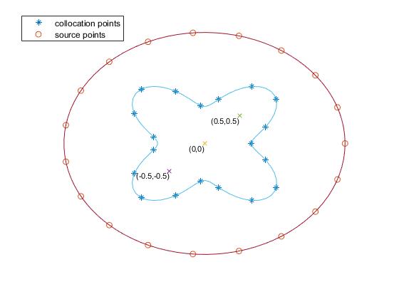
Figure 1: Collocation, interior, and source points for Example 5.1.

Then setting $u_{n}=0$ in Equation (17) gives us the numerical solution to problem (39)-(40). Equation (39) is a modified Helmholtz equation for which the maximum principle applies. So to estimate the numerical error we choose $150$ points $\mathbf{z}_{k}\in\partial\Omega$ corresponding to equally spaced points in $[0,2\pi]$ and calculate

$$\text{error}=\max_{1\leq k\leq 150}|u_{e}(\mathbf{z}_{k})-u_{N}(\mathbf{z}_{k})|.$$

Furthermore, we compare the numerical solution with the exact solution at the interior points of $\Omega$ shown in Figure 1: $(0,0),(-0.5,-0.5)$, and $(0.5,0.5)$. Then our results are presented below for different values of $N$ and $a$.

Table 1: Numerical errors on $\partial\Omega$ for Example 5.1

$a$ Value	$N=30$	$N=40$	$N=50$
$a=5$	5.7834e-08	1.7858e-04	1.8384e-05
$a=6$	6.4251e-08	1.5524e-04	3.0641e-04
$a=7$	7.6068e-08	3.2974e-04	2.1189e-04

Table 2: Numerical errors at $(0,0)\in\Omega$ for Example 5.1

$a$ Value	$N=30$	$N=40$	$N=50$
$a=5$	1.2697e-09	3.7395e-05	2.0255e-06
$a=6$	3.6321e-09	2.6167e-05	4.5180e-06
$a=7$	7.2834e-09	3.8662e-05	7.6944e-06

Table 3: Numerical errors at $(-0.5,-0.5)\in\Omega$ for Example 5.1

$a$ Value	$N=30$	$N=40$	$N=50$
$a=5$	3.3531e-09	1.4115e-05	3.6029e-06
$a=6$	1.0839e-08	5.9511e-05	3.6455e-05
$a=7$	2.6621e-09	8.7411e-05	6.5502e-06

Table 4: Numerical errors at $(0.5,0.5)\in\Omega$ for Example 5.1

$a$ Value	$N=30$	$N=40$	$N=50$
$a=5$	1.8178e-10	7.0093e-05	5.2808e-06
$a=6$	1.2718e-09	1.5910e-05	9.0011e-05
$a=7$	1.1732e-08	3.2128e-06	6.7437e-05

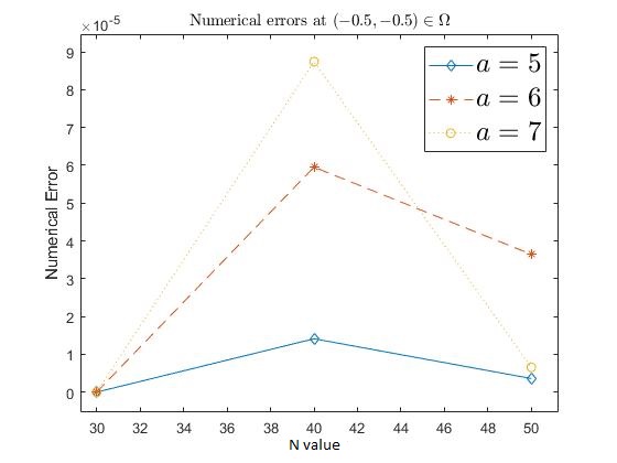
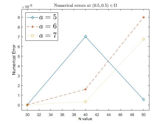
Figure 2: Example 5.1 errors on $\partial\Omega$ and $3$ interior points

Next we use MFS and MPS to solve a non-homogeneous Helmholtz problem.

Example 5.2.

Consider

$$\Delta u(x,y)-u(x,y) =2xe^{y},\quad (x,y)\in\Omega,$$ (41)

$$u(x,y) =xye^{y},\quad (x,y)\in\partial\Omega.$$ (42)

where $\Omega=\{(x,y):x^{2}+y^{2}<1\}$. The exact solution to this problem is given by $u_{e}(x,y)=xye^{y}$. For the non-homogeneous Helmholtz equation, we use the approximate particular solutions discussed in §2. Here we use different RBFs, $\phi_{1}(r)=\sqrt{\frac{c}{\pi}}e^{-cr^{2}}$ and $\phi_{2}(r)=\frac{35}{32}(1-r^{2})^{3}\chi_{[-1,1]}(r)$, where $\chi$ is the characteristic function. And use points of the form $\frac{\mathbf{j}}{n}=(\frac{k}{n},\frac{m}{n})$ in $\Omega_{\delta}$, $k,m\in\mathbb{Z}$ to get the approximate solutions from Equation (13).

Next, we use the methods in MFS to solve problem (15)-(16), as discussed before. We obtain $N$ collocation points by plugging in $N$ equally spaced points of $[0,2\pi]$ into $(\cos{t},\sin{t})$, and use a fictitious domain $\partial{\widetilde{\Omega}}$ whose boundary is given by the polar equation

$$r=5-\cos{6\theta},$$

for $\theta\in[0,2\pi]$. We get $N$ source points by plugging into the above polar equation.

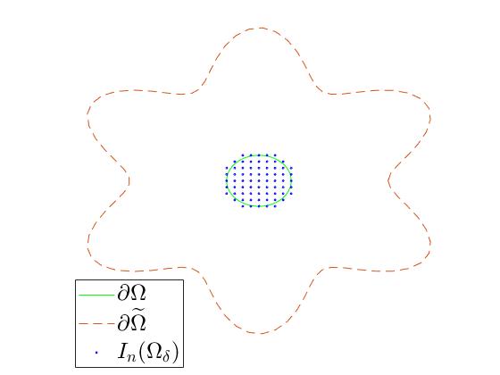
Figure 3: Domains and points of $I_{n}(\Omega_{\delta})$ for Example 5.2

Then the numerical solution to the original problem is given by Equation (17). To estimate the error we calculate

$$\text{error}=\max_{1\leq i\leq 450}{|u_{e}(\mathbf{z}_{i})-u_{n}(\mathbf{z}_{i})|}$$

where $u_{n}$ is the numerical solution to the original problem, and $\mathbf{z}_{i}$, $1\leq i\leq 450$, consists of $350$ points in $\Omega$ and $100$ points on $\partial\Omega$. The interior points for estimating the errors are obtained by plugging into the polar equation $r=(1/14)\theta$, for $2\pi\leq\theta\leq 4\pi$, and the boundary points are obtained by plugging into $(\cos{t},\sin{t})$. The results are given in the tables below.

Table 5: Errors for Example 5.2 with $\phi(r)=\sqrt{\frac{c}{\pi}}e^{-cr^{2}}$, $n=14$, and $\delta=0.2$

$c$ Value	$N=30$	$N=40$	$N=50$
$c=3.77$	9.8458e-04	9.0813e-04	9.4048e-04
$c=3.8$	6.8730e-04	6.2337e-04	6.6379e-04
$c=3.82$	4.9107e-04	4.3522e-04	4.8256e-04

Table 6: Errors for Example 5.2 with $\phi(r)=\sqrt{\frac{c}{\pi}}e^{-cr^{2}}$, $n=24$, and $\delta=0.1$

$c$ Value	$N=30$	$N=40$	$N=50$
$c=4$	1.9549e-03	1.9259e-03	1.9475e-03
$c=4.2$	9.4343e-04	8.7272e-04	9.5018e-04
$c=4.4$	2.5448e-03	2.4606e-03	2.5349e-03

Table 7: Errors for Example 5.2 with $\phi_{2}(r)=\frac{35}{32}(1-r^{2})^{3}\chi_{[-1,1]}(r)$ and $\delta=0.2$

$n$ Value	$N=30$	$N=40$	$N=50$
$n=16$	1.4661e-03	1.4744e-03	1.4839e-03
$n=30$	2.3721e-03	2.3513e-03	2.3640e-03
$n=50$	9.7023e-04	9.7664e-04	1.0239e-03

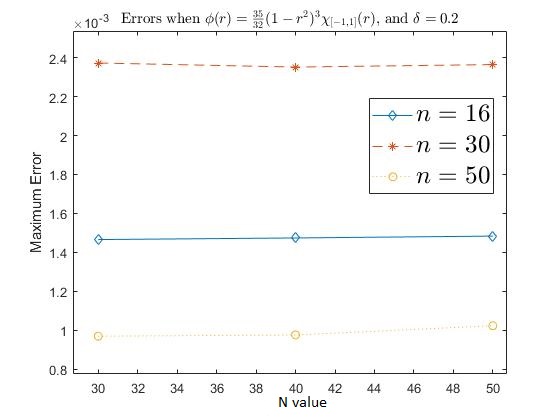
Figure 4: Example 5.2 errors for different RBFs, $n$, and $c$ values

Now we use the particular solution in Equation (14) for a 3D problem.

Example 5.3.

Consider the following problem in $\mathbb{R}^{3}$

$$\Delta u(x,y,z)-u(x,y,z) =2ye^{z},\quad (x,y,z)\in\Omega,$$ (43)

$$u(x,y,z) =x^{2}ye^{z},\quad (x,y,z)\in\partial\Omega.$$ (44)

where $\Omega=\{(x,y,z):x^{2}+y^{2}+z^{2}<1\}$ is the unit sphere. The exact solution of this problem is $u_{e}(x,y,z)=x^{2}ye^{z}$. We use the Gaussian function $\phi(r)=\sqrt{0.1/\pi}e^{-0.1r^{2}}$ as our RBF. Then we use points of the form $\frac{\mathbf{j}}{n}=(\frac{k}{n},\frac{m}{n},\frac{l}{n})$ in $\Omega_{\delta}$, $k,m,l\in\mathbb{Z}$ to get the approximate solutions from Equation (14). We use $N$ collocation points and $N$ source points on a sphere of radius $4$ centered at the origin. The the numerical solution to problem (43)-(44) is given by Equation (17).

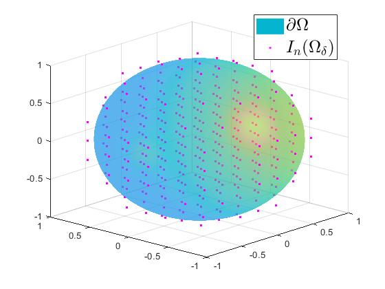
Figure 5: The boundary $\partial\Omega$ and points in $I_{n}(\Omega_{\delta})$ for Example 5.3

Error estimates are calculated as in the previous examples. We calculate the maximum error at $686$ boundary points and the numerical error at $3$ interior points. The results are given below.

Table 8: Errors on $\partial\Omega$ for Example 5.3 with $\delta=0.2$

$n$ Value	$N=155$	$N=176$	$N=203$
$n=5$	8.8797e-04	5.8049e-04	1.0279e-03
$n=10$	5.7091e-04	3.0869e-04	8.3734e-05
$n=20$	4.8601e-04	2.5440e-04	1.0339e-04

Table 9: Errors at $(0.26,0,-0.15)\in\Omega$ for Example 5.3 with $\delta=0.2$

$n$ Value	$N=155$	$N=176$	$N=203$
$n=5$	1.3216e-04	2.9446e-05	1.2316e-04
$n=10$	7.63554e-05	1.2761e-06	1.3956e-05
$n=20$	3.4145e-05	1.5425e-05	1.3176e-05

Table 10: Errors at $(0.26,0,0.15)\in\Omega$ for Example 5.3 with $\delta=0.2$

$n$ Value	$N=155$	$N=176$	$N=203$
$n=5$	1.5254e-04	1.9090e-05	1.2736e-04
$n=10$	1.0593e-04	8.1219e-06	2.2554e-05
$n=20$	6.2453e-05	2.6541e-05	2.2394e-05

Table 11: Errors at $(0,0,0.3)\in\Omega$ for Example 5.3 with $\delta=0.2$

$n$ Value	$N=155$	$N=176$	$N=203$
$n=5$	8.2412e-05	4.6458e-05	5.4867e-05
$n=10$	6.4257e-05	2.32639e-05	1.3766e-05
$n=20$	5.10585e-05	2.5940e-05	1.3930e-05

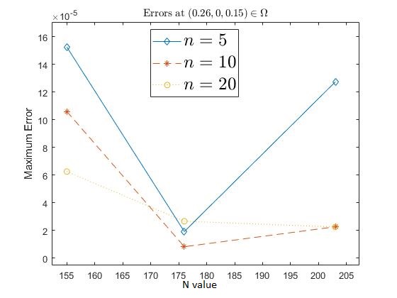
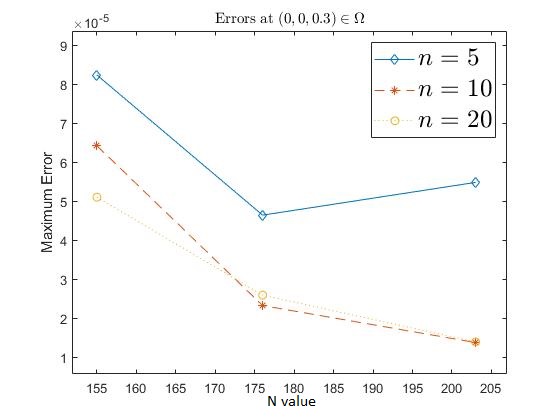
Figure 6: Example 5.3 errors on $\partial\Omega$ and $3$ interior points

Next we use the Laplace transform for a diffusion problem.

Example 5.4.

Consider the following diffusion problem on a square with boundary temperatures at zero. A similar example can be found in [21].

$$\frac{1}{k}\frac{\partial u}{\partial t}(x,y,t) =\Delta u(x,y), (x,y)\in\Omega,\quad t>0,$$ (45)

$$u(x,y,t) =0, (x,y)\in\partial\Omega,\quad t>0,$$

$$u(x,y,0) =1, (x,y)\in\Omega,\quad t=0.$$

where $\Omega=(-0.1,0.1)\times(-0.1,0.1)$ and $k=5.8\times 10^{-7}$ $m^{2}/s$. The analytical solution to this problem is given by

$$u_{e}(x,y,t)=\frac{16}{\pi^{2}}\sum_{n,m=1}^{\infty}A_{n,m}e^{\lambda_{n,m}t}\cos{\frac{(2n+1)\pi x}{0.2}}\cos{\frac{(2m+1)\pi y}{0.2}},$$ (46)

where

$$A_{n,m}=\frac{(-1)^{n+m}}{(2n+1)(2m+1)},$$

and

$$\lambda_{n,m}=-\frac{k\pi^{2}}{0.04}\big{(}(2n+1)^{2}+(2m+1)^{2}\big{)}.$$

Since the initial condition is harmonic we can apply the change of variable $v(x,y,t)=u(x,y,t)-u(x,y,0)$, which leads to the following problem

$$\frac{\partial v}{\partial t}(x,y,t) =\Delta v(x,y), (x,y)\in\Omega,\quad t>0,$$ (47)

$$v(x,y,t) =-1, (x,y)\in\partial\Omega,\quad t>0,$$

$$v(x,y,0) =0, (x,y)\in\Omega,\quad t=0.$$

Now we take the Laplace transform of the above problem, as mentioned in §3, to obtain the following Helmholtz problem

$$\Delta V(x,y,s_{l})-s_{l}V(x,y,s_{l}) =0,\quad (x,y)\in\Omega,$$ (48)

$$V(x,y,s_{l}) =-1/s_{l},\quad (x,y)\in\partial\Omega,$$ (49)

where $V(x,y,s_{l})=\mathscr{L}[v(x,y,t)]$, and the values for $s_{l}$, $1\leq l\leq n_{s}$, are given in Equation (24) where we choose $n_{s}=10$ and $18$, and a time $t=9000$ to evaluate the original problem at. Then for each $s_{l}$ we solve problem (48)-(49) using the MFS and MPS where we use $40$ equally spaced points on $\partial\Omega$ as the collocation points and $40$ equally spaced source points on the circle centered at the origin with radius $2$ (See Figure 7). Next we approximate the inverse Laplace transform by Equation (25) to get the numerical solution $\widetilde{v}(x,y,t)$ to the problem (47). Finally the numerical solution to the original problem (45) is given by $\widetilde{u}(x,y,t)=\widetilde{v}(x,y,t)+u(x,y,0)$.

We compare the exact solution with the numerical solution at $6$ points $(x,y)\in\Omega$, and calculate the error as follows

$$\text{Error}=|u(x,y,9000)-\widetilde{u}(x,y,9000)|.$$

The results are given in the tables below.

Table 12: True and numerical solutions to Example 5.4 with $n_{s}=10$

$(x,y)\in\Omega$	True Solution	Numerical Solution	Error
$(-0.01,0.07)$	0.7014	0.7521	0.0507
$(-0.01,0.04)$	0.7682	0.8034	0.0351
$(-0.01,0.01)$	0.8008	0.8026	1.7366e-03
$(-0.01,-0.01)$	0.8008	0.8001	7.3928e-04
$(-0.01,-0.04)$	0.7682	0.7966	0.0283
$(-0.01,-0.07)$	0.7014	0.7929	0.0915

Table 13: True and numerical solutions to Example 5.4 with $n_{s}=18$

$(x,y)\in\Omega$	True Solution	Numerical Solution	Error
$(-0.01,0.07)$	0.7014	0.7921	0.0906
$(-0.01,0.04)$	0.7682	0.7934	0.0251
$(-0.01,0.01)$	0.8008	0.7926	8.2685e-03
$(-0.01,-0.01)$	0.8008	0.7901	0.0107
$(-0.01,-0.04)$	0.7682	0.7866	0.0183
$(-0.01,-0.07)$	0.7014	0.7829	0.0814

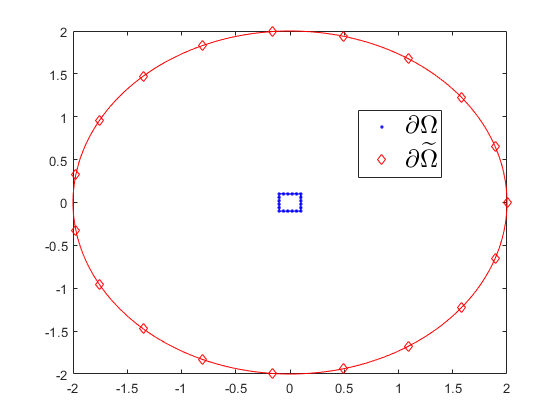
Figure 7: Collocation and source points for Example 5.4

Example 5.5.

We now revisit problem (45) in Example 5.4, but use the difference in time methods. Recall the analytical solution to this problem is given by Equation (46).

First we choose $M$ equally spaced points on the time interval $[0,T]$ so that we can form the approximation of the time derivative $\frac{\partial u}{\partial t}(x,y,n\tau)$ given in Equation (30), where $\tau=t/n$, and $n=1,2,\cdots,M$. Next, we rearrange terms so that our problem becomes the inhomogeneous Helmholtz problem mentioned in Equation (35). Then we use the methods in §2 to solve the Helmholtz equation subject to the boundary and initial conditions in (45). Here we use $\phi(r)=\sqrt{3/\pi}e^{-3r^{2}}$ as our RBF, and choose $\delta=0.2$ and use points of the form $\frac{\mathbf{j}}{l}=(\frac{k}{l},\frac{m}{l})$ in $\Omega_{\delta}$, $k,m\in\mathbb{Z}$, $l=14$, to get the approximate solutions from Equation (13). Next, the methods in §2 are used to solve problem (15)-(16). $40$ collocation and source points are chosen in the same manner as in Example 5.4 (see Figure 8). Finally, the solution, $\widetilde{u}_{n}(x,y)$ to the problem (35) subject to the initial and boundary conditions in (45) is given by Equation (17). By repeating this process in an iterative manner we can find $\widetilde{u}_{2}(x,y)$, $\widetilde{u}_{3}(x,y)$, $\cdots$, $\widetilde{u}_{M}(x,y)$.

We evaluate the numerical solution, $\widetilde{u}_{M}$, and the true solution, $u$, at the same $6$ interior points $(x,y)\in\Omega$ and $T$ value used in Example 5.4. The results are presented below for different values of $M$.

Table 14: True and numerical solutions to Example 5.5 with $M=10$

$(x,y)\in\Omega$	True Solution	Numerical Solution	Error
$(-0.01,0.07)$	0.7014	0.7211	0.0197
$(-0.01,0.04)$	0.7682	0.7666	1.5999e-03
$(-0.01,0.01)$	0.8008	0.7976	3.1984e-03
$(-0.01,-0.01)$	0.8008	0.8121	0.0113
$(-0.01,-0.04)$	0.7682	0.7721	3.9114e-03
$(-0.01,-0.07)$	0.7014	0.7112	9.8114e-03

Table 15: True and numerical solutions to Example 5.5 with $M=30$

$(x,y)\in\Omega$	True Solution	Numerical Solution	Error
$(-0.01,0.07)$	0.7014	0.7112	9.8321e-03
$(-0.01,0.04)$	0.7682	0.7567	0.0114
$(-0.01,0.01)$	0.8008	0.8100	9.2124e-03
$(-0.01,-0.01)$	0.8008	0.8025	1.7231e-03
$(-0.01,-0.04)$	0.7682	0.7694	1.2234e-03
$(-0.01,-0.07)$	0.7014	0.7100	8.6241e-03

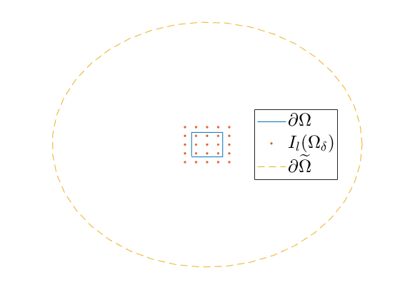
Figure 8: Domains and points in $I_{l}(\Omega_{\delta})$ for Example 5.5

Next, we look at a wave problem using the Laplace transform.

Example 5.6.

Consider the following model of a vibrating rectangular membrane.

$$\frac{\partial^{2}u}{\partial t^{2}}(x,y,t) =\Delta u(x,y,t), (x,y)\in\Omega,\quad t>0,$$ (50)

$$u(x,y,t) =0, (x,y)\in\partial\Omega,\quad t>0,$$

$$\frac{\partial u}{\partial t}(x,y,0) =xy, (x,y)\in\Omega,\quad t=0,$$

$$u(x,y,0) =0, (x,y)\in\Omega,\quad t=0.$$

where $\Omega=(0,1)\times(0,1)$. Using the separation of variables method we find that the analytical solution to this problem is given by

$$u_{e}(x,y,t)=\sum_{m=1}^{\infty}\sum_{n=1}^{\infty}\frac{4(-1)^{m+n}}{\pi^{2}mn\lambda_{m,n}}\sin{(\lambda_{m,n}t)}\sin{(m\pi x)}\sin{(n\pi y)},$$ (51)

where

$$\lambda_{m,n}=\pi\sqrt{m^{2}+n^{2}}.$$

After applying the Laplace transform to the above problem, we choose $10$ fixed values $s_{l}$, $1\leq l\leq 10$, to be the Laplace transform parameters mentioned in Equation (24), and then we obtain the following Helmholtz BVP

$$\Delta U(\mathbf{x})-s_{l}^{2}U(\mathbf{x}) =xy,\quad \mathbf{x}\in\Omega,$$ (52)

$$U(\mathbf{x}) =0,\quad \mathbf{x}\in\partial\Omega,$$ (53)

where $U(\mathbf{x})=\mathscr{L}[u(x,y,t)](s_{l})$. For each $s_{l}$, problem (52)-(53) can be solved by the methods in §2. We will use $\phi(r)=\sqrt{\frac{10}{\pi}}e^{-10r^{2}}$ as our RBF, $\delta=0.1$, and $n=16$. Then we use points of the form $\frac{\mathbf{j}}{n}=(\frac{k}{n},\frac{m}{n})$ in $\Omega_{\delta}$, $k,m\in\mathbb{Z}$ to get the approximate solutions from Equation (13). Next, we choose $N$ collocation points to be equally spaced points on $\partial\Omega$ and $N$ source points to be equally spaced points on a circle of radius $1.2$ whose center is $(0.5,0.5)$. Then the numerical solution to the problem (52)-(53) is given by Equation (17). Lastly, to find the numerical solution to the original problem (50) we use the formula for the inverse Laplace transform as mentioned above.

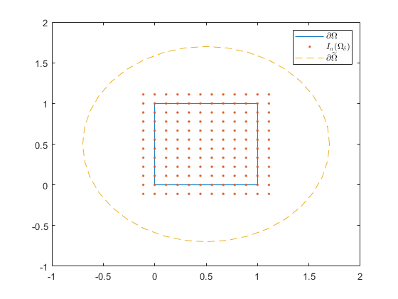
Figure 9: Domains and points used for Example 5.6

To estimate the numerical error we will choose $6$ points $(x,y)\in\Omega$, and a time $t=T$, then calculate

$$\text{error}=|u(x,y,T)-u_{e}(x,y,T)|.$$

The errors are presented below for different values of $N$ and $T$.

Table 16: Numerical errors to Example 5.6 with $N=29$

$(x,y)\in\Omega$	T= 15	T=20
$(0.14,0.35)$	7.8634e-03	2.0180e-03
$(0.29,0.35)$	6.0318e-03	0.0266
$(0.43,0.35)$	7.7390e-03	0.0647
$(0.57,0.35)$	0.0424	0.0523
$(0.71,0.35)$	0.0728	0.0343
$(0.86,0.35)$	0.0586	0.0212

Table 17: Numerical errors to Example 5.6 with $N=37$

$(x,y)\in\Omega$	T= 15	T=20
$(0.14,0.35)$	9.0618e-04	4.2558e-03
$(0.29,0.35)$	0.0257	0.0398
$(0.43,0.35)$	0.0180	0.0819
$(0.57,0.35)$	0.0446	0.0828
$(0.71,0.35)$	0.0716	0.0732
$(0.86,0.35)$	0.0547	0.0416

Example 5.7.

Let us revisit problem (50), but here we use the difference in time approach. Recall the analytical solution to this problem is given by Equation (51).

First we choose $M$ equally spaced points on the time interval $[0,T]$ for some $T$. Then we use the methods in §2 to solve Equation (36) subject to the initial conditions (37) and boundary condition (38). We use $\phi(r)=\sqrt{3/\pi}e^{-3r^{2}}$ as our RBF. We choose $\delta=0.2$ and use points of the form $\frac{\mathbf{j}}{l}=(\frac{k}{l},\frac{m}{l})$ in $\Omega_{\delta}$, $k,m\in\mathbb{Z}$, $l=14$, to get the approximate solutions from Equation (13). Next, the methods in §2 are used to solve problem (15)-(16). $N$ equally spaced points on $\partial\Omega$ are used as the collocation points. The source points are $N$ equally spaced points on a circle of radius $1.2$ with center $(0.5,0.5)$. Finally, the solution, ${u}_{n}(x,y)$ to the problem (36) with initial conditions (37) and boundary condition (38) is given by Equation (17). Then repeating this process in an iterative manner we can find $u_{3}(x,y)$, $u_{4}(x,y)$, $\cdots$, $u_{M}(x,y)$.

To get the numerical error, we choose $6$ points $(x,y)\in\Omega$ and calculate

$$\text{error}=|u_{e}(x,y,T)-u_{M}(x,y,T)|,$$

where $u_{e}$ is the exact solution. The results are presented below for different values of $T$, $M$, and $N$.

Table 18: Numerical errors to Example 5.7 with $N=21$ and $M=15$

$(x,y)\in\Omega$	T= 5	T=15
$(0.14,0.35)$	0.0197	0.0138
$(0.29,0.35)$	0.0151	5.0604e-05
$(0.43,0.35)$	6.1836e-03	1.0821e-03
$(0.57,0.35)$	0.0377	0.0343
$(0.71,0.35)$	0.0260	0.0615
$(0.86,0.35)$	8.3917e-03	0.0350

Table 19: Numerical errors to Example 5.7 with $N=157$ and $M=10$

$(x,y)\in\Omega$	T= 5	T=15
$(0.14,0.35)$	7.4234e-04	0.0146
$(0.29,0.35)$	0.0239	8.7654e-04
$(0.43,0.35)$	0.0171	8.0491e-04
$(0.57,0.35)$	3.0332e-03	0.0355
$(0.71,0.35)$	9.9534e-03	0.0660
$(0.86,0.35)$	7.9493e-03	0.0521

Table 20: Numerical errors to Example 5.7 with $N=157$ and $M=15$

$(x,y)\in\Omega$	T= 5	T=15
$(0.14,0.35)$	1.1104e-04	8.8195e-04
$(0.29,0.35)$	0.0225	0.0214
$(0.43,0.35)$	0.0155	0.0143
$(0.57,0.35)$	1.3922e-03	1.4931e-04
$(0.71,0.35)$	0.0113	0.0124
$(0.86,0.35)$	8.8048e-03	9.5762e-03

6.   Conclusions

We investigated diffusion and wave initial boundary value problems by transforming the respective problems into Helmholtz boundary value problems and then using a meshless approach to solve the problems. One of the motivations for using meshless methods is its simplicity in implementation. As shown in the examples above, many of the problems can be solved using relatively few points.

References

- [1] M.A. Golberg and C.S. Chen, "The Method of Fundamental Solutions for Potential, Helmholtz and Diffusion Problems," in Boundary Integral Methods: Numerical and Mathematical Aspects, vol. 1, WIT press Southampton, 1998, pp. 103-176.
- [2] X. Li, "Radial Basis Approximation for Newtonian Potentials," Advances in Computational Mathematics, vol. 33, no. 1, 2010.
- [3] X. Li, "Convergence of the Method of Fundamental Solutions for Poisson’s Equation on the Unit Sphere," Advances in Computational Mathematics, vol. 28, no. 3, pp. 269-282, 2008, Springer.
- [4] G. Fairweather and A. Karageorghis, "The method of fundamental solutions for elliptic boundary value problems," Advances in Computational Mathematics, vol. 9, no. 1, pp. 69-95, 1998, Springer.
- [5] M. Choi, "Meshless Methods for Numerically Solving Boundary Value Problems of Elliptic Type Partial Differential Equations," Ph.D. dissertation, UNLV, 2018.
- [6] S. Zhu, P. Satravaha, and X. Lu, "Solving linear diffusion equations with the dual reciprocity method in Laplace space," Engineering Analysis with Boundary Elements, vol. 13, no. 1, pp. 1-10, 1994, Elsevier.
- [7] G.J. Moridis and D.L. Reddel, "The Laplace transform boundary element (LTBE) method for the solution of diffusion-type equations," in Boundary Elements XIII, pp. 83-97, Springer, 1991.
- [8] H. Stehfest, "Algorithm 368: Numerical inversion of Laplace transforms [D5]," Communications of the ACM, vol. 13, no. 1, pp. 47-49, 1970, ACM New York, NY, USA.
- [9] X. Li, "Approximation of potential integral by radial bases for solutions of Helmholtz equation," Advances in Computational Mathematics, vol. 30, no. 3, pp. 201-230, 2009, Springer.
- [10] Z.C. Li, Y. Wei, Y. Chen, and H.T. Huang, "The method of fundamental solutions for the Helmholtz equation," Applied Numerical Mathematics, vol. 135, pp. 510-536, 2019, Elsevier.
- [11] D.L. Young, S.C. Jane, C.Y. Lin, C.L. Chiu, and K.C. Chen, "Solutions of 2D and 3D Stokes laws using multiquadrics method," Engineering Analysis with Boundary Elements, vol. 28, no. 10, pp. 1233-1243, 2004, Elsevier.
- [12] V. Popov and T. Bui, "A meshless solution to two-dimensional convection–diffusion problems," Engineering Analysis with Boundary Elements, vol. 34, no. 7, pp. 680-689, 2010, Elsevier.
- [13] C.S. Chen, X. Jiang, W. Chen, and G. Yao, "Fast Solution for Solving the Modified Helmholtz Equation with the Method of Fundamental Solutions," Communications in Computational Physics, vol. 17, no. 3, pp. 867-886, 2015, Cambridge University Press.
- [14] A. Karageorghis, D. Lesnic, and L. Marin, "A survey of applications of the MFS to inverse problems," Inverse Problems in Science and Engineering, vol. 19, no. 3, pp. 309-336, 2011, Taylor & Francis.
- [15] X. Li, "Radial basis approximation and its application to biharmonic equation," Advances in Computational Mathematics, vol. 32, no. 3, pp. 275-302, 2010, Springer.
- [16] C.S. Chen, A. Karageorghis, and F. Dou, "A novel RBF collocation method using fictitious centres," Applied Mathematics Letters, vol. 101, p. 106069, 2020, Elsevier.
- [17] X. Zhu, F. Dou, A. Karageorghis, and C.S. Chen, "A fictitious points one–step MPS–MFS technique," Applied Mathematics and Computation, vol. 382, p. 125332, 2020, Elsevier.
- [18] M.A. Jankowska, A. Karageorghis, and C.S. Chen, "Improved Kansa RBF method for the solution of nonlinear boundary value problems," Engineering Analysis with Boundary Elements, vol. 87, pp. 173-183, 2018, Elsevier.
- [19] S.R. Karur and P.A. Ramachandra, "Radial basis function approximation in the dual reciprocity method," Mathematical and Computer Modelling, vol. 20, no. 7, pp. 59-70, 1994, Elsevier.
- [20] A.S. Muleshkov, C.S. Chen, M.A. Golberg, and A.H.-D. Cheng, "Analytic Particular Solutions for Inhomogeneous Helmholtz-Type Equations," Advances in Computational Engineering & Sciences, vol. 1, pp. 27-32, 2000, Tech Science Press.
- [21] C.S. Chen, "Lecture Note Laplace Transform for Solving Linear Diffusion Equations."