The deuterium fractionation of NH₃ in massive star-forming regions

Abstract

Deuteration is sensitive to environmental conditions in star-forming regions. To investigate NH₂D chemistry, we compared the spatial distribution of ortho-NH₂D $1_{11}^{s}-1_{01}^{a}$, NH₃(1,1) and NH₃(2,2) in 12 late-stage massive star-forming regions. By averaging several pixels along the spatial slices of ortho-NH₂D $1_{11}^{s}-1_{01}^{a}$, we obtained the deuterium fractionation of NH₃. In seven targets, the deuterium fractionation of NH₃ shows a decreasing trend with increasing rotational temperature. This trend is less clear in the remaining five sources, likely due to limited spatial resolution. However, when considering all 12 sources together, the anticorrelation between NH₃ deuterium fractionation and rotational temperature becomes less significant, suggesting that other physical parameters may influence the fractionation. Additionally, we found that the region of highest deuterium fractionation of NH₃ is offset from the NH₃ peak in each source, likely because the temperature is higher near the NH₃ peaks and NH₂D may be depleted from the gas phase as the molecular cloud core evolves, as well as the increased release of CO from grains into the gas phase.

1 Introduction

The abundances of molecules in which one or more hydrogen atoms have been replaced by deuterium are regarded as good indicators of the evolutionary stages of interstellar molecular clouds (e.g. Crapsi et al., 2005; Emprechtinger et al., 2009; Fontani et al., 2011). Due to their lower zero-point energies compared to their hydrogen-containing counterparts, the formation of deuterated species, such as DCN, DCO⁺, N₂D⁺ and NH₂D, is favored at low temperatures (Herbst, 1982). The ratio of a deuterated species to their hydrogen-containing counterparts, known as deuterium fractionation ($D_{\rm frac}$), can be several orders of magnitude higher than the D/H ratio ($\approx$1.5 $\times$ 10^-5) in the interstellar medium (ISM) (Linsky et al., 1995; Oliveira et al., 2003). Consequently, the abundance of these deuterated molecules is often found to be enhanced (e.g. Busquet et al., 2010; Hsu et al., 2021; Jensen et al., 2021).

The formation of deuterated ammonia, NH₂D, NHD₂ and ND₃, is often considered to be associated with deuterated ions, such as H₂D⁺ and CH₂D⁺, which convert ammonia (NH₃) in the gas phase (e.g. Rodgers & Charnley, 2001; Caselli et al., 2008; Caselli & Ceccarelli, 2012; Ceccarelli et al., 2014). Chemical reactions on the surfaces of dust grains also contribute to the production of deuterated ammonia (e.g. Turner, 1990; Caselli et al., 2008; Ceccarelli et al., 2014; Fontani et al., 2015). Additionally, the abundance of deuterated species could be affected by shocks (Lis et al., 2002).

NH₂D was first detected in Sgr B2 (Turner et al., 1978) and Orion KL (Rodriguez Kuiper et al., 1978). Despite decades of observations and modeling, our understanding of deuterium chemistry remains limited (Öberg et al., 2021). Several studies have been carried out to investigate the relationship between $D_{\rm frac}$(NH₃) and rotation temperature (e.g. Neill et al., 2013; Fontani et al., 2015; Wienen et al., 2021). With single-pointing observations using single-dish telescopes, no clear trend has been obtained for the relationship between $D_{\rm frac}$(NH₃) and $T_{\rm rot}$(2,2;1,1) (e.g. Fontani et al., 2015; Wienen et al., 2021). For instance, Fontani et al. (2015) reported that no clear correlation between $D_{\rm frac}$(NH₃) and ammonia rotation temperature is found with Institut de Radioastronomie Milli${\rm\acute{m}}$etrique (IRAM) and Green Bank Telescope (GBT) observations toward 28 massive star-forming regions in different evolutionary stages. Similarly, with IRAM observations toward 992 ATLASGAL (APEX Telescope Large Area Survey) massive clumps, Wienen et al. (2021) also reported a flat distribution of $D_{\rm frac}$(NH₃) and ammonia rotation temperature.

However, several interferometric images from case studies provide observational evidence that $D_{\rm frac}$(NH₃) is influenced by temperature. Busquet et al. (2010) found that the $D_{\rm frac}$(NH₃) in young stellar objects (YSOs) was lower than in pre-protostellar cores using IRAM Plateau de Bure Interferometer (PdBI) observations. Additionally, Neill et al. (2013) suggested that a slightly warmer environment results in lower deuterium fractionation by comparing $D_{\rm frac}$(NH₃) in the hot core and compact ridge of Orion KL using Atacama Large Millimeter/submillimeter Array (ALMA) observations.

Single-pointing observations using single-dish telescopes lack the spatial distribution of $D_{\rm frac}$(NH₃), while interferometric observations often focus on one or two targets, which limits the ability to compare the relationship between temperature and $D_{\rm frac}$(NH₃) with different physical environments. Therefore, conducting single-dish mapping toward a relatively large sample, the spatial distribution of NH₃ and NH₂D could enhance our understanding of the deuterium chemistry of NH₃ in massive star-forming regions.

In Li et al. (2024), we obtained the spatial distribution of ortho-NH₂D $1_{11}^{s}-1_{01}^{a}$ at 85.926 GHz in 18 Galactic late-stage massive star-forming regions with IRAM 30 m. We found that the spatial distribution of ortho-NH₂D $1_{11}^{s}-1_{01}^{a}$ at 85.926 GHz is complex and differs from the dense gas tracer H¹³CN 1-0. To further investigate deuterium fractionation and conduct a more comprehensive study of singly deuterated ammonia (hereafter deuterated ammonia), we performed a line study of ortho-NH₂D $1_{11}^{s}-1_{01}^{a}$ at 85.926 GHz, NH₃(1,1) at 23.696 GHz and NH₃(2,2) at 23.722 GHz toward 12 Galactic late-stage massive star-forming regions in this work. The data include ortho-NH₂D $1_{11}^{s}-1_{01}^{a}$ at 85.926 GHz for 12 sources as presented in Li et al. (2024), as well as NH₃(1,1) and NH₃(2,2) data for three sources observed with Effelsberg 100 m. Additionally, NH₃(1,1) and NH₃(2,2) data for the remaining nine sources were obtained from GBT 100 m archival data.

In this work, we compared the spatial distributions between ortho-NH₂D $1_{11}^{s}-1_{01}^{a}$, NH₃(1,1) and NH₃(2,2) maps in late-stage massive star-forming regions. $D_{\rm frac}$(NH₃) is derived for each source and is utilized to analyze its relationship with temperature. The observations are described in Section 2, the main results are reported in Section 3, a discussion is given in Section 4, and a brief summary is given in Section 5.

2 Observations and data reduction

2.1 NH₃ data

2.1.1 Effelsberg 100 m observation

The ammonia inversion transitions, NH₃(1,1) and NH₃(2,2) were observed toward G081.75+00.59, G109.87+00.77 and G121.29+00.65 during 2021 February and 2023 July with Effelsberg 100 m telescope. The beam size of Effelsberg is 42.5^′′ at 23 GHz. The secondary focus receiver S14mm Double Beam RX with a bandwidth of 300 MHz was used during our observation. The Fast Fourier Transform Spectrometer (XFFTS) was used with 65536 channels, providing a frequency resolution of 4.6 kHz and a velocity resolution of 0.058 km s^-1. The system temperatures were 100–140 K during our observation. In the following analysis, the velocity resolution is smoothed to about 0.6 km s^-1 with a frequency resolution of 46 kHz at 23 GHz. The on-the-fly (OTF) mapping was used for this observation. A strong continuum source, NGC 7027, was used to calibrate the spectral line flux. The typical rms are about 0.2 K at 0.6 km s^-1. The details of each source are listed in Table 1.

2.1.2 GBT 100 m archival data

We retrieved the data for NH₃(1,1) and NH₃(2,2) of nine sources from the GBT archive, and the beam size of GBT is 31.8^′′ at 23 GHz. The observations of all GBT archival data have been made using the $K$-band Focal Plane Array (KFPA) receiver.

The NH₃(1,1) and NH₃(2,2) data of G034.39+00.22, G035.19-00.74 and G075.76+00.33 from Urquhart et al. (2015) were used. The velocity resolution was also smoothed to about 0.6 km s^-1 and the rms in $T_{\rm mb}$ is about 0.02 K for each source.

The NH₃(1,1) and NH₃(2,2) data of G023.44-00.18 and G031.28+00.06 from the Radio Ammonia Mid-Plane Survey (RAMPS; Hogge et al. 2018) were used. The velocity resolution was smoothed to about 0.6 km s^-1 with about 0.05 K rms in $T_{\rm mb}$ for each source.

In four sources, G015.03-00.67, G035.20-01.73, G081.87+00.78 and G111.54+00.77, NH₃(1,1) and NH₃(2,2) data from KFPA Examinations of Young STellar Object Natal Environments (KEYSTONE; Keown et al. 2019) were used. The velocity resolution was smoothed to about 0.6 km s^-1 with 0.03 K rms in $T_{\rm mb}$ for each source.

2.2 NH₂D data

For sources mentioned in Section 2.1, we used the ortho-NH₂D $1_{11}^{s}-1_{01}^{a}$ data that were presented in Li et al. (2024). These ortho-NH₂D $1_{11}^{s}-1_{01}^{a}$ data were observed by IRAM 30 m with a beam size of about 28.6^′′ at 86 GHz. The typical rms are about 0.05 K at 0.6 km s^-1, corresponding to 195 kHz frequency resolution at 86 GHz. The specific observing parameters are described in Li et al. (2024).

2.3 Data reduction

The lines used consist of ortho-NH₂D $1_{11}^{s}-1_{01}^{a}$ at 85.926 GHz, NH₃(1,1) at 23.696 GHz and NH₃(2,2) at 23.722 GHz. Data reduction was conducted with GILDAS software. The angular resolution of the IRAM 30 m telescope is about 28.6^′′ at 86 GHz, while the angular resolutions of the Effelsberg 100 m telescope and GBT 100 m telescope are about 42.5^′′ and 31.8^′′, respectively, at 23 GHz.

For G081.75+00.59, G109.87+00.77 and G121.29+00.65, in which the NH₃ data were obtained from Effelsberg 100 m observation, the ortho-NH₂D $1_{11}^{s}-1_{01}^{a}$ data were smoothed to match the Effelsberg resolution of 42.5^′′. For these three sources, the ortho-NH₂D $1_{11}^{s}-1_{01}^{a}$, NH₃(1,1) and NH₃(2,2) data were regridded to steps of 14^′′ (about 1/3 beam size) with a beam size of 42.5^′′.

For the other nine sources, in which NH₃ data were obtained from GBT archival data, the ortho-NH₂D $1_{11}^{s}-1_{01}^{a}$, NH₃(1,1) and NH₃(2,2) data were regridded to steps of 9^′′ (about 1/3 beam size) with a beam size of 30^′′ . First-order baselines were used for all spectra. In the following analysis, the beam filling factor is assumed to be unity.

3 Results

3.1 Velocity-integrated intensity maps of ortho-NH₂D $1_{11}^{s}-1_{01}^{a}$, NH₃(1,1) and NH₃(2,2)

In cold environment, the five components of ortho-NH₂D $1_{11}^{s}-1_{01}^{a}$ can often be distinguished (e.g. Crapsi et al., 2007; Li et al., 2021; Saito et al., 2000). However, due to the line broadening in late-stage massive star forming regions, three components are blended and only three can be distinguished with single-dish observations (Pazukhin et al., 2023; Pillai et al., 2007). Therefore, the fluxes of ortho-NH₂D $1_{11}^{s}-1_{01}^{a}$ were derived with the velocity-integrated intensity of the emitting channels of its six hyperfine structures instead of Gaussian fitting. For NH₃(1,1) and NH₃(2,2), the main group was used to derive the velocity-integrated intensity. The NH₃(1,1) and NH₃(2,2) maps present a clear structure for each source. The ortho-NH₂D $1_{11}^{s}-1_{01}^{a}$, NH₃(1,1) and NH₃(2,2) velocity-integrated intensity maps for G035.19-00.74 are shown in Figure 1, while other sources are shown in Figures B1-B12.

From the velocity-integrated intensity maps of ortho-NH₂D $1_{11}^{s}-1_{01}^{a}$, NH₃(1,1) and NH₃(2,2), half of the sources (G031.28+00.06, G034.39+00.22, G035.19-00.74, G081.87+00.78, G109.87+02.11 and G111.54+00.77), showed morphological differences in spatial distribution between ortho-NH₂D $1_{11}^{s}-1_{01}^{a}$ and NH₃(1,1) (or NH₃(2,2)). Even though the ortho-NH₂D $1_{11}^{s}-1_{01}^{a}$ and NH₃ emissions can be resolved in G121.29+00.65, no clear difference can be found for the spatial distribution of these lines. For the remaining five sources (G015.03-00.67, G023.44-00.18, G035.20-01.73, G075.76+00.33 and G081.75+00.59), the differentiation in distribution between ortho-NH₂D $1_{11}^{s}-1_{01}^{a}$ and NH₃(1,1) (or NH₃(2,2)) is less apparent owing to the limited spatial resolution.

3.2 Temperature and column density

Two ammonia inversion transitions, NH₃(1,1) and NH₃(2,2), were obtained in 12 sources with Effelsberg observations and GBT archival data. Based on the methods of Ho & Townes (1983) and Mangum et al. (1992) for calculating NH₃ parameters, Lu et al. (2015) provided a Python package to fit the NH₃ spectra and obtained NH₃ parameters, including the rotation temperature $T_{\rm rot}$(2,2;1,1), which represents the population between NH₃(1,1) and NH₃(2,2) (Ho & Townes, 1983), and the optical depth of NH₃(1,1) main group ($\tau$(1,1,m)).

At local thermodynamic equilibrium (LTE), the column density can be given by

$$N_{tot}=\frac{3h}{8\pi^{3}S\mu^{2}\nu}Q(T_{ex})e^{E_{u}/kT_{ex}}\int T^{\prime}_{mb}d\nu(cm^{-2}),$$ (1)

where $h=6.624\times 10^{-27}$erg$\cdot$s is the Planck constant, $\nu$ is the frequency of the transition, $E_{u}$ is the energy of the upper level, $S$ is the line strength, and $\mu^{2}$ is the dipole moment. The values of these parameters for ortho-NH₂D $1_{11}^{s}-1_{01}^{a}$, NH₃(1,1) and NH₃(2,2) are listed in Table 2. $\int T^{\prime}_{mb}d\nu$ is the velocity-integrated intensity with optical depth correction, given by Goldsmith & Langer (1999):

$$\int T^{\prime}_{mb}d\nu=\int T_{mb}d\nu\frac{\tau}{1-e^{-\tau}},$$ (2)

where $\int T_{mb}d\nu$ is the velocity-integrated intensity from observation.

The rotation temperature of ammonia, $T_{\rm rot}$(2,2;1,1), is assumed to be equal to the excitation temperature of ammonia, $T_{\rm ex}$. The NH₃ partition function is determined by considering the contribution of the different metastable levels (from $J,K$=0,0 to $J,K$=6,6), which are given by CDMS (Müller et al., 2001, 2005). Based on the above assumptions, the column density of NH₃ can be derived by Eq.1.

For NH₂D, the excitation temperature cannot be derived, as only one transition was observed. Therefore, the rotation temperature of ammonia is assumed to be the excitation temperature of NH₂D. In regions with relatively low density, the ortho-NH₂D $1_{11}^{s}-1_{01}^{a}$ may not be thermalized, meaning that $T_{\rm ex}$ is not equal to $T_{\rm rot}$. According to our checks, this assumption of $T_{\rm ex}$=$T_{\rm rot}$ results in at most a 15% error if the $T_{\rm ex}$ of ortho-NH₂D $1_{11}^{s}-1_{01}^{a}$ exceeds 10 K. The ortho/para ratio of NH₂D is assumed to be 3 (Tiné et al., 2000), and we assume that the ortho-NH₂D $1_{11}^{s}-1_{01}^{a}$ line is optically thin. The NH₂D partition function is also determined by considering the contributions of different energy levels (from $J$=0 to $J$=9), as obtained from CDMS (Müller et al., 2001, 2005). Using Eq.1, the column density of NH₂D could be derived.

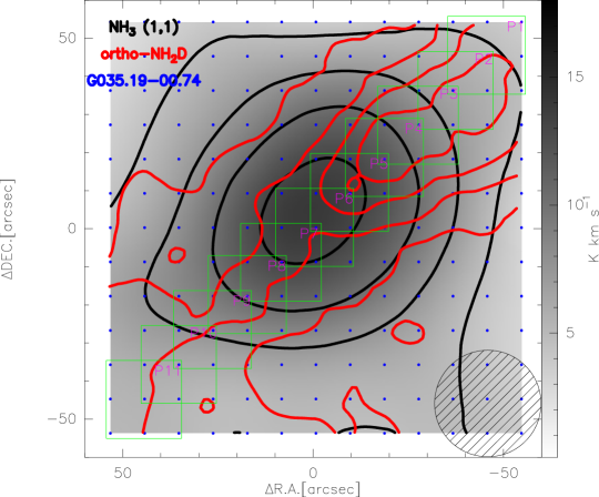
Figure 2: The pixels in the box are the average area in G035.19-00.74. The order of the region numbers is the order in Table 1.

To improve the signal-to-noise ratio of NH₃(1,1), NH₃(2,2) and ortho-NH₂D $1_{11}^{s}-1_{01}^{a}$, several pixels were averaged. For G081.75+00.59, G109.87+00.77 and G121.29+00.65, where the NH₃ data were obtained from Effelsberg 100 m observations, 4 pixels were averaged. In the other nine sources, 9 pixels were averaged. The method of pixel averaging for one of the sources is presented in Figure 2, and other sources are shown in Figure D1. In Figure 2 (and Figure D1), the pixels in the green box are used for averaging. After reducing the spatial resolution, the column density and rotation temperature are listed in Table 1. In the following analysis, column density and rotation temperature with reduced spatial resolution were used.

3.3 Deuterium fractionation of NH₃

Assuming that the NH₂D emission and NH₃ emission originate from the same region, the deuterium fractionation of NH₃ is derived from the column densities of NH₃ and NH₂D listed in Table 1, which is calculated after reducing the spatial resolution as mentioned in Section 3.2. In the following analysis, $D_{\rm frac}$(NH₃) with reduced spatial resolution was used.

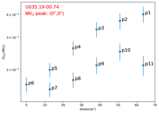
Figure 3: The relationship between deuterium fractionation of NH₃ and distance of NH₃ peak in G035.19-00.74.

The relationship between deuterium fractionation of NH₃ and distance of NH₃ peak in G035.19-00.74 is presented in Figure 3, while other sources are shown in Figure E1. Multiple data points at the same distance occur because different locations share the same distance from the NH₃ peak. For the six sources in which the spatial distribution of NH₃(1,1) differs from that of ortho-NH₂D $1_{11}^{s}-1_{01}^{a}$, the location of the highest deuterium fractionation of NH₃ is offset from the NH₃ peak.

The highest deuterium fractionation of NH₃ (0.086$\pm$0.007) in the entire sample is found in G081.87+00.78 with offset (45^′′,9^′′), while the NH₃ peak is located in offset (0^′′,0^′′). G111.54+00.77 exhibits the largest range of $D_{\rm frac}$(NH₃), varying from 0.014$\pm$0.002 to 0.067$\pm$0.010. In contrast, for other sources, the variation in $D_{\rm frac}$(NH₃) exceeds a factor of two, except G031.28+00.06, G035.20-01.73 and G075.76+00.33, for which the variation in $D_{\rm frac}$(NH₃) is below a factor of two. The ranges and medians of $T_{\rm rot}$ and $D_{\rm frac}$(NH₃) for each source are listed in Table 3.

3.4 Individual target detail

3.4.1 G015.03-00.67

G015.03-00.67 (M17) is a molecular cloud complex (Lada, 1976) with one of the most luminous giant cometary HII regions in the Galaxy (3.6$\times$10⁶$L_{\sun}$; Povich et al. 2009). It is the closest (1.98 kpc, Xu et al. 2011) giant HII region to the sun. More than 100 OB-type massive young stellar objects have been found in G015.03-00.67 (Lada et al., 1991; Povich et al., 2009). Zhu et al. (2023) found that the shocked gas is spreading near the boundary of the M17 HII region, likely due to the expansion of ionized gas.

In the southwest of M17 with a 4^′$\times$4^′ size, the distributions of NH₃(1,1) and NH₃(2,2) and ortho-NH₂D $1_{11}^{s}-1_{01}^{a}$ were obtained (see Figure B1). A widely distributed NH₃(1,1) and NH₃(2,2) are detected, while the emission of ortho-NH₂D $1_{11}^{s}-1_{01}^{a}$ presents a fragmented distribution and weak emission. G015.03-00.67 is the source with the lowest deuterium fractionation in our sample. In this target, the region with the highest deuterium fractionation is located south of G015.03-00.67. The range of $D_{\rm frac}$(NH₃) is from 0.0051$\pm$0.0008 to 0.012$\pm$0.002 in G015.03-00.67.

3.4.2 G023.44-00.18

With a strong 6.7 GHz CH₃OH maser detected, G023.44-00.18 is thought to have young massive stars inside (Walsh et al., 1998). Ren et al. (2011) reported that G023.44-00.18 has two dust cores arranged north and south, based on the Submillimeter Array (SMA) observation. They suggested that these two dust cores are in the pre-UCHII evolutionary stage, with outflow detected in the southern one. Using PdBI observations, Zhang et al. (2020) found several NH₂D cores in G023.44-00.18 with high $D_{\rm frac}$(NH₃)$\gtrsim$ 0.3, but these cores are offset from the two dust cores.

Due to the spatial resolution limitation, these NH₂D cores cannot be distinguished in the present work (see Figure B2). The ortho-NH₂D $1_{11}^{s}-1_{01}^{a}$, NH₃(1,1) and NH₃(2,2) are not detected as asymmetrically distributed spatial structures in the mapping center. Therefore, a series of similar deuterium fractionations are derived in G023.44-00.18. However, the highest $D_{\rm frac}$(NH₃) was detected in the northwestern region of G023.44-00.18. We derived a $D_{\rm frac}$(NH₃) range from 0.009$\pm$0.001 to 0.031$\pm$0.006 in this target.

3.4.3 G031.28+00.06

G031.28+00.06 is embedded in the molecular cloud complex W43 (Nguyen Luong et al., 2011). With Very Large Array (VLA) 6 cm continuum imaging, Fey et al. (1992) found a ring emission in G031.28+00.06. Additionally, IRAM 30m observations detected H42$\alpha$ in G031.28+00.06, indicating the presence of an HII region (Li et al., 2024).

NH₃(1,1) and NH₃(2,2) exhibit a northeast-to-southwest distribution. But the ortho-NH₂D $1_{11}^{s}-1_{01}^{a}$ emission presents two structures (see Figure B3) and seems to be separated by the HII region, which is reported in Li et al. (2024). The center of the spatial distribution of NH₃(1,1) and NH₃(2,2) is located in the middle of two NH₂D structures. The range of $D_{\rm frac}$(NH₃) is from 0.009$\pm$0.001 to 0.013$\pm$0.002 in this source.

3.4.4 G034.39+00.22

G034.39+00.22 stretches about 9$\arcmin$ from north to south based on IRAM 30m 1.2 mm continuum observation (Rathborne et al., 2006). With VLA ammonia observation, Miralles et al. (1994) reported that G034.39+00.22 contains a total mass of about 1000 $M_{\sun}$. Additionally, using the Nobeyama Radio Observatory (NRO) 45 m telescope observation, Sakai et al. (2012) derived the D_frac(HNC) to be about 0.003.

We obtain a north-south distribution of NH₃(1,1), NH₃(2,2) and ortho-NH₂D $1_{11}^{s}-1_{01}^{a}$ of 2$\arcmin$$\times$2$\arcmin$ size in G034.39+00.22. The NH₃(1,1), NH₃(2,2) and ortho-NH₂D $1_{11}^{s}-1_{01}^{a}$ show distinct structures aligned along the north-south axis, without significant asymmetry in the east-west direction (see Figure B4). The deuterium fractionation of NH₃ in the southern structure is higher than that in the northern structure. In G034.39+00.22, the range of $D_{\rm frac}$(NH₃) is from 0.017$\pm$0.002 to 0.035$\pm$0.003.

3.4.5 G035.19-00.74

G035.19-00.74 contains a young B0 star (Dent et al., 1984). A CO outflow was detected in this source with an orientation of approximately 45^∘ along the northeast-southwest direction with James Clerk Maxwell Telescope (JCMT) observations (Gibb et al., 2003). NH₃ mapping with VLA observations revealed the presence of a rotating interstellar disk with a mass of about 150 $M_{\sun}$ in G035.19-00.74 (Little et al., 1985), which is perpendicular to the CO outflow reported by Gibb et al. (2003).

In G035.19-00.74, strong ortho-NH₂D $1_{11}^{s}-1_{01}^{a}$ emission is detected in the southeast and northwest regions, while the NH₃ peak is located at the center of the map. Therefore, the high deuterium fractionation of NH₃ is located in the southeast and northwest regions, while the deuterium fractionation of NH₃ is relatively low in the NH₃ peak. We derived a $D_{\rm frac}$(NH₃) range from 0.016$\pm$0.001 to 0.040$\pm$0.004 in this source.

3.4.6 G035.20-01.73

G035.20-01.73 (W 48) contains a 2$\arcmin$$\times$2$\arcmin$ HII region (Wood & Churchwell, 1989; Roshi et al., 2005). With Herschel and Berkeley Illinois Maryland Association (BIMA) interferometer observations, Rygl et al. (2014) reported an east-west evolutionary gradient within this UCHII region. For G035.20-01.73, it was found that the 3.5 mm dust emission peak does not coincide with the brightest NH₂D peak with PdBI observations (Pillai et al., 2011).

The east-west distributions of ortho-NH₂D $1_{11}^{s}-1_{01}^{a}$, NH₃(1,1) and NH₃(2,2) are present in G035.20-01.73 (see Figure B6). The ortho-NH₂D $1_{11}^{s}-1_{01}^{a}$ emission is located in the west of G035.20-01.73 and shows a similar distribution to the result in Pillai et al. (2011). In contrast, the emission of ortho-NH₂D $1_{11}^{s}-1_{01}^{a}$, NH₃(1,1) and NH₃(2,2) is weaker in the east of G035.20-01.73, where the UCHII region is located (Rygl et al., 2014). There is also an east-west gradient in the deuterium fractionation of NH₃, increasing farther away from the UCHII region. The range of $D_{\rm frac}$(NH₃) is from 0.024$\pm$0.003 to 0.041$\pm$0.004 in G035.20-01.73.

3.4.7 G075.76+00.33

G075.76+00.33 is located in the giant molecular cloud ON2 (Matthews et al., 1973). An UCHII region in the north of G075.76+00.33 was reported by Wood & Churchwell (1989).

The northeast-to-southwest distributions of ortho-NH₂D $1_{11}^{s}-1_{01}^{a}$, NH₃(1,1) and NH₃(2,2) are presented in Figure B7. However, the ortho-NH₂D $1_{11}^{s}-1_{01}^{a}$, NH₃(1,1) and NH₃(2,2) emissions are not associated with the UCHII region as reported in (Wood & Churchwell, 1989). This target exhibits the narrowest range of $D_{\rm frac}$(NH₃) in our sample, ranging from 0.018$\pm$0.2 to 0.023$\pm$0.003.

3.4.8 G081.75+00.59

G081.75+00.59 (DR 21) is a giant star-forming complex in the Cygnus X molecular cloud complex (Dickel et al., 1978; Kirby, 2009) with about 25$\arcmin$-length ridge based on Herschel observations(Motte et al., 2007; Hennemann et al., 2012). It contains several YSOs and high-mass protostars (e.g. Harvey et al., 1986; Mangum et al., 1991; Motte et al., 2007). With IRAM observation, Christensen et al. (2023) reported an extended distribution of ortho-NH₂D $1_{11}^{s}-1_{01}^{a}$, DCN 1-0, DNC 1-0 and DCO⁺ 1-0 in Cygnus X.

We obtain a similar ortho-NH₂D $1_{11}^{s}-1_{01}^{a}$ distribution to that reported in Christensen et al. (2023) (see Figure B8). In G081.75+00.59, the abundance of NH₃ increases from north to south, whereas the NH₂D abundance decreases along the same direction. We derived a $D_{\rm frac}$(NH₃) range from 0.022$\pm$0.002 to 0.068$\pm$0.008 in G081.75+00.59.

3.4.9 G081.87+00.78

North of G081.75+00.59, G081.87+00.78 (W75N) is another massive star-forming region in the Cygnus X molecular cloud complex (Dickel et al., 1978; Persi et al., 2006). This target is reported to host a large-scale, high-velocity molecular outflow (Shepherd et al., 2003) and contains a B-type YSO (Shepherd et al., 2004).

The ortho-NH₂D $1_{11}^{s}-1_{01}^{a}$, NH₃(1,1) and NH₃(2,2) present a southeast-to-northwest distribution in G081.87+00.78, while ortho-NH₂D $1_{11}^{s}-1_{01}^{a}$ is predominantly located to the east of NH₃(1,1) and NH₃(2,2) (see figure B9). G081.87+00.78 has the highest deuterium fractionation of NH₃ (0.086$\pm$0.007) in our sample. Besides, the range of $D_{\rm frac}$(NH₃) is from 0.036$\pm$0.003 to 0.086$\pm$0.007 in this source.

3.4.10 G109.87+02.11

With several YSOs detected, G109.87+02.11 (Cep A) is an active massive star-forming region (Hughes & Wouterloot, 1984). HW2, the brightest radio source in G109.87+02.11, is associated with a zero-age main-sequence (ZAMS) star of early B spectral type (Hughes & Wouterloot, 1984). With IRAM 30 m observations, Li et al. (2017) detected strong ortho-NH₂D emission in the northeast of G109.87+02.11, suggesting that the abundance of NH₂D may be associated with shock.

As is shown in Figure B10, strong ortho-NH₂D $1_{11}^{s}-1_{01}^{a}$ emission is detected in the northeast of G109.87+02.11, while NH₃(1,1) and NH₃(2,2) are weak, indicating high deuterium fractionation in this region. We derived a $D_{\rm frac}$(NH₃) range from 0.011$\pm$0.002 to 0.055$\pm$0.023 in this target.

3.4.11 G111.54+00.77

G111.54+00.77 (NGC 7538) is a massive star-forming region located in a giant molecular cloud complex (Ungerechts et al., 2000) and is associated with a HII region (e.g. Luisi et al., 2016; Sharma et al., 2017; Beuther et al., 2022). With Herschel observations, several high-mass dense clump candidates were identified in G111.54+00.77, which are expected to produce several intermediate-to-high-mass stars in the future (Fallscheer et al., 2013). The mass of gas and dust in this target is estimated to be several thousand solar masses (Reid & Wilson, 2005).

In G111.54+00.77, widespread distributions of ortho-NH₂D $1_{11}^{s}-1_{01}^{a}$, NH₃(1,1) and NH₃(2,2) have been detected (see figure B11). NH₃(1,1) and NH₃(2,2) are predominantly detected in the southern region, whereas ortho-NH₂D $1_{11}^{s}-1_{01}^{a}$ is more concentrated in the southwest, indicating a high deuterium fractionation in the southwest of G111.54+00.77. This target exhibits the widest range of $D_{\rm frac}$(NH₃) in our sample, ranging from 0.014$\pm$0.002 to 0.067$\pm$0.010.

3.4.12 G121.29+00.65

With the detection of 6.7 GHz CH₃OH, G121.29+00.65 (L1287) is forming a massive star (Rygl et al., 2010). A bipolar outflow oriented in the northeast-southwest direction was observed through SMA observations (Juárez et al., 2019).

The distributions of ortho-NH₂D $1_{11}^{s}-1_{01}^{a}$, NH₃(1,1) and NH₃(2,2) are shown in Figure B12. Both NH₂D and NH₃ exhibit distributions that are perpendicular to the bipolar outflow as reported by (Juárez et al., 2019). The ortho-NH₂D $1_{11}^{s}-1_{01}^{a}$, NH₃(1,1) and NH₃(2,2) show a northwest-to-southeast distribution. Similar to G035.19-00.74, the high deuterium fractionation in G121.29+00.65 is detected in the southeastern and northwestern regions, while it is relatively low in the mapping center, where the NH₃ peak is located. The range of $D_{\rm frac}$(NH₃) is from 0.020$\pm$0.003 to 0.041$\pm$0.014 in this target.

4 Discussion

4.1 Environmental impact of the enrichment of deuterated ammonia

Seven targets, G031.28+00.06, G034.39+00.22, G035.19-00.74, G081.87+00.78, G109.87+02.11, G111.54+00.77 and G121.29+00.65, exhibit an anticorrelation between $D_{\rm frac}$(NH₃) and $T_{\rm rot}$(2,2;1,1) within each source (see Figure 4). This anticorrelation indicates that $D_{\rm frac}$(NH₃) is influenced by temperature, with $D_{\rm frac}$(NH₃) decreasing as temperature increases in these seven targets. Such anticorrelation was reported in case studies with interferometric observations (Busquet et al., 2010; Neill et al., 2013). Therefore, the temperature could indeed be an important physical parameter to influence the deuterium fractionation of NH₃. For the other five targets, G015.03-00.67, G023.44-00.18, G035.20-01.73, G075.76+00.33 and G081.75+00.59, the relationship between $D_{\rm frac}$(NH₃) and $T_{\rm rot}$(2,2;1,1) could not be analyzed owing to limitations in spatial resolution and sensitivity. Our 12 targets are classified based on the presence or absence of clear anticorrelation between $D_{\rm frac}$(NH₃) and $T_{\rm rot}$(2,2;1,1), as listed in Table 3.

However, no clear trend of the relation between $D_{\rm frac}$(NH₃) and $T_{\rm rot}$(2,2;1,1) is evident when analyzing all data across 12 targets together (see Figure 4). Furthermore, there is no clear trend between $D_{\rm frac}$(NH₃) and $T_{\rm rot}$(2,2;1,1) exhibited in either one of the groups even when considered separately, regardless of the presence or absence of a clear anticorrelation between $D_{\rm frac}$(NH₃) and $T_{\rm rot}$(2,2;1,1) (see also Figure 4). Similar results were reported by Pazukhin et al. (2023), where no correlation between $D_{\rm frac}$(NH₃) and $T_{\rm rot}$(2,2;1,1) was found when considering five high-mass star-forming regions as a whole, based on IRAM 30 m and Effelsberg 100 m observations. Such a result is somehow also consistent with that from single-pointing observations using single-dish telescopes (Fontani et al., 2015; Wienen et al., 2021). Physical parameters, such as ionization rate, density and evolutionary stage, vary among sources, which could contribute to the lack of a clear relationship between $D_{\rm frac}$(NH₃) and temperature when analyzing a large sample.

H₂D⁺ plays a key role in deuterium fractionation processes (e.g. Pagani et al., 1992; Emprechtinger et al., 2009; Caselli & Ceccarelli, 2012; Ceccarelli et al., 2014). In cold molecular gas, the chemical model shows that the abundance ratio of H₂D⁺ to H${}^{+}_{3}$ drops rapidly when the gas kinetic temperature is above $\sim$ 15 K (Caselli et al., 2008), leading to reduced deuterium fractionation as temperature rises. However, $D_{\rm frac}$(NH₃) may be influenced not only by temperature but also by other physical parameters. To understand how $D_{\rm frac}$(NH₃) is influenced by other physical parameters, we constructed a chemical model that considers different physical parameters, including temperature, density, cosmic-ray ionization rates and evolutionary timescales.

4.2 Chemical model

The chemical model used in this work is the DNAUTILUS gas-grain chemical model, an updated version of the NAUTILUS model (Reboussin et al., 2014; Ruaud et al., 2015; Wakelam et al., 2015a) described in Majumdar et al. (2017). This code solves for the time dependent abundances of molecules, in both two-phase mode, which treats the entire grain as chemically homogeneous, and three-phase mode, which treats the grain surface and bulk as chemically distinct. This chemical model considers the gas- and grain-phase chemical species from the KIDA network(Wakelam et al., 2015b), including multiply deuterated isotopologues. The chemical network consists of 15 elements, all of which are listed with their initial abundances in Table 4. Only H₂ and HD exist in molecular form, while the other elements remain in atomic form. Elements such as C, S, Si, Fe, Na, Mg, Cl and P, whose ionization potential is less than 13.6 eV, appear as singly positive ions. Though the model can handle the spin chemistry of H₂, H${}_{2}^{+}$, H${}_{3}^{+}$, and their corresponding deuterated isotopologues, the present network includes deuteration up to 14 atoms without considering the spin of any H- or D-bearing species. This simplification is necessary for simplicity and computational efficiency given the large parameter space that we choose to explore in this work. The network includes 1606 gas species, 1472 grain surface species, and 1472 grain-mantle species linked by 83715 gas-phase reactions, 10,967 reactions on grain surfaces, and 9431 reactions in the grain mantles. More details are described in Majumdar et al. (2017).

To obtain the deuterium fractionation of NH₃ varying with temperature, the model was run with dust and gas temperatures ranging from 6 K to 60 K, in the steps of 2 K. To account for different physical environments, the model was run with varying proton densities ($n_{\mathrm{H}}$) and cosmic-ray ionization rates ($\zeta$). Specifically, the proton densities were set to 10⁴ cm^-3, 10⁵ cm^-3, 10⁶ cm^-3 and 10⁷ cm^-3, and the cosmic-ray ionization rates to 3$\times$10^-18 s^-1, 1.5$\times$10^-17 s^-1, 3$\times$10^-17 s^-1, 6$\times$10^-17 s^-1 and 3$\times$10^-16 s^-1. A proton density of n_H=10⁶ cm^-3 is typical for hot cores (e.g. van Dishoeck & Blake, 1998; Kurtz et al., 2000), and $\zeta$=3$\times$10^-17 s^-1 is the average cosmic-ray ionization rate measured in massive star-forming regions by van der Tak & van Dishoeck (2000). A visual extinction of 10 mag was used in each simulation. According to our tests, visual extinction does not significantly impact the simulation results. The physical parameters used in our simulation are listed in Table 5.

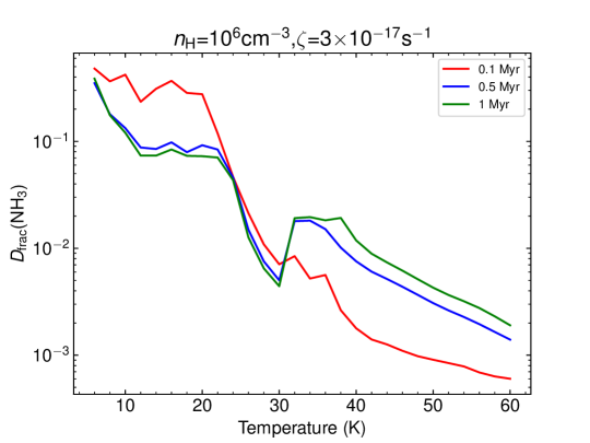
Figure 5: Deuterium fractionation of NH₃ as a function of temperature simulated by the gas-grain chemical model. The timescales for the red, blue and green lines are 0.1, 0.5 and 1 Myr, respectively.

The simulation results are present in Figure 5-8. In Figure 5, with a fixed proton density $n_{\mathrm{H}}$=10⁶ cm^-3) and cosmic-ray ionization rate ($\zeta$=3$\times$10^-17 s^-1), there is only a slight difference between the different timescales (0.1, 0.5 and 1 Myr) regarding the relationship between the deuterium fractionation of NH₃ and temperature. $D_{\rm frac}$(NH₃) generally decreases as temperature increases, though this trend is not strictly monotonic. A “bulge” in $D_{\rm frac}$(NH₃) is seen between 30 and 40 K before continuing its downward trend with higher temperatures. Some major production and destruction pathways of NH₃ and NH₂D, in which the reactions have a contribution of at least $\textgreater$ 10%, are listed in table 6. For all temperatures $T$ up to 60 K considered in the simulation, the electron recombination reaction (equation 3) remains a significant pathway for the production of NH₃ and NH₂D:

$$\text{NH}_{4}^{+}/\text{NH}_{3}\text{D}^{+}+\text{e}^{-}\rightarrow\text{H}+\text{NH}_{3}/\text{NH}_{2}\text{D}.$$ (3)

However, the destruction pathways of NH₃ and NH₂D evolve as temperature increases, influencing the NH₂D/NH₃ ratios. The pathways are primarily dominated by various ion-molecule reactions, as shown in Table 6. At lower temperatures ($T$ $\lesssim$ 24 K), the pathways involving H₃⁺ and H⁺ are the major ones. However, as the temperature increases ($T$ $\gtrsim$ 24 K), other competing reactions involving HCO⁺ and H₃O⁺ become more favorable, with minor contributions from N₂H⁺, S⁺, and the depletion of NH₃ on grain surfaces.

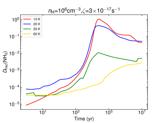
Figure 6: Deuterium fractionation of NH₃ as a function of timescale simulated by the gas-grain chemical model. The timescales for the red, blue, green and yellow lines are 10, 20, 30 and 60 K, respectively.

With a fixed proton density $n_{\mathrm{H}}$=10⁶ cm^-3) and cosmic-ray ionization rate ($\zeta$=3$\times$10^-17 s^-1), the simulation results between $D_{\rm frac}$(NH₃) and timescale are presented in Figure 6. $D_{\rm frac}$(NH₃) evolves over time, initially showing an increasing trend before beginning to decrease at about 10⁴ yr.

In Figure 7, with a fixed cosmic-ray ionization rate ($\zeta$=3$\times$10^-17 s^-1), no clear trend is found among different densities in the relationship between deuterium fractionation of NH₃ and temperature. Except for temperatures above 30 K at 0.1 Myr in our simulations, different densities lead to variations of a factor of several or even dozens in deuterium fractionation of NH₃. Furthermore, at 0.5 and 1 Myr, no clear relationship between density and deuterium fractionation of NH₃ is evident. However, at 0.1 Myr, the simulation results indicate a high deuterium fractionation of NH₃ at high densities and low temperatures.

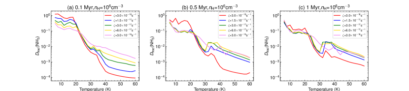
Figure 8: Deuterium fractionation of NH₃ as a function of temperature for different cosmic-ray ionization rates simulated by the gas-grain chemical model. The cosmic-ray ionization rate for the red, blue, green, yellow and violet lines is 3$\times$10^-18, 1.5$\times$10^-17, 3$\times$10^-17, 6$\times$10^-17 and 3$\times$10^-16 s^-1 respectively. The timescales for the left, middle and right panels are 0.1r, 0.5 and 1 Myr, respectively. The cosmic-ray ionization rate is set to $n_{\rm H_{2}}$=10⁶ cm^-3 for each model.

With a fixed proton density n_H=10⁶ cm^-3), there is a clear difference among different cosmic-ray ionization rates in the relationship between deuterium fractionation of NH₃ and temperature (see Figure 8). Except for temperature at 20-26K, different cosmic-ray ionization rates can lead to variations of a factor of several or even dozens in deuterium fractionation of NH₃. At the timescale of 0.1 Myr, the deuterium fractionation of NH₃ increases as the ionization rate decreases when temperatures are below 20 K, but it increases with higher cosmic-ray ionization rates when temperatures exceed 30 K. However, at the timescales of 0.5 Myr and 1 Myr, the relationship between deuterium fractionation of NH₃ and cosmic-ray ionization rate becomes more complex, making it difficult to determine the exact influence of cosmic-ray ionization rate on deuterium fractionation of NH₃.

4.3 Comparison between chemical model and observation

Most targets present a trend of increasing $D_{\rm frac}$(NH₃) with decreasing temperature, while this trend becomes unclear when all 12 targets are considered as a whole. According to our chemical model, when using consistent values for density, cosmic-ray ionization rates and timescale, $D_{\rm frac}$(NH₃) is high at low temperature ($T$$\lesssim$20 K) and low at high temperature ($T$$\gtrsim$50 K) (see Figure 5). This suggests an anticorrelation between $D_{\rm frac}$(NH₃) and temperature, explaining why most targets in this study, along with interferometric observations (e.g. Busquet et al., 2010; Neill et al., 2013) show a trend of increasing $D_{\rm frac}$(NH₃) with decreasing temperature.

Our targets are located in different physical environments. As described in Section 3.4, although all targets are late-stage massive star-forming regions, there are slight differences in their evolutionary stages. For instance, G015.03-00.67 is a giant HII region (Lada, 1976) and is associated with over 100 OB-type massive young stellar objects (Lada et al., 1991; Povich et al., 2009), whereas G121.29+00.65 is forming a massive star (Rygl et al., 2010). With IRAM 30m observations, dense gas tracer H¹³CN 1-0 was mapped for our sources (Li et al., 2024), but the velocity-integrated intensity of H¹³CN 1-0 differs among the sources. This suggests that the sources may have different densities.

At the same temperature, our chemical model shows that different timescales, proton densities, or cosmic-ray ionization rates can lead to varying $D_{\rm frac}$(NH₃) (see Figure 5-8). This indicates that different physical environments can lead to different $D_{\rm frac}$(NH₃). Consequently, when all 12 targets are considered collectively, there is no clear relationship between $D_{\rm frac}$(NH₃) and temperature.

In brief, $D_{\rm frac}$(NH₃) generally tends to decrease with increasing temperature. But $D_{\rm frac}$(NH₃) is influenced not only by temperature but also by other physical parameters.

Limited by the evolutionary stage of the sample, we lack information on the early evolutionary stages. Additionally, our observation lacks other spectral lines that are unable to estimate the effect of different cosmic-ray ionization rates on $D_{\rm frac}$(NH₃). Combined with the early-stage massive star-forming regions and ionization degree tracer (such as HCO⁺, N₂H⁺ and their deuterated counterparts; Caselli et al. 1998; Caselli 2002), the future work could provide further insights into how $D_{\rm frac}$(NH₃) is influenced by different physical environments.

4.4 Nonoverlap between NH₃ and $D_{\rm frac}$(NH₃) peaks

The location of the highest deuterium fractionation of NH₃ deviates from the NH₃ peak in almost all sources, regardless of whether there is a difference in morphology between the spatial distribution of ortho-NH₂D $1_{11}^{s}-1_{01}^{a}$ and NH₃(1,1) (or NH₃(2,2)) or not. Although the location of the highest deuterium fractionation of NH₃ deviates from the NH₃ peak by less than 20$\arcsec$ in G035.20-01.73 and G075.76+00.33, the NH₃ and $D_{\rm frac}$(NH₃) peaks still may not be colocated.

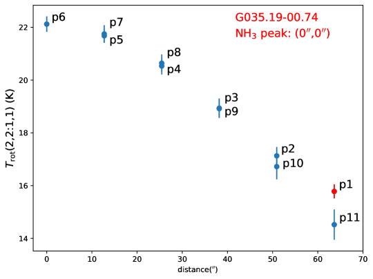
Figure 9: The relationship between rotation temperature of NH₃ and distance of NH₃ peak in G035.19-00.74. The red marker is the position with the highest deuterium fractionation of NH₃.

As shown in Figure 9, the temperature decreases with increasing distance from the NH₃ peak in G035.19-00.74, while other sources are shown in Figure E2. Only one source, G075.76+00.33 presents that the highest value of $D_{\rm frac}$(NH₃) and the highest rotation temperature are situated in the same position. The reason may be that the differentiation in the distribution of ortho-NH₂D $1_{11}^{s}-1_{01}^{a}$ and NH₃(1,1) (or NH₃(2,2)) is less apparent owing to the limited spatial resolution. In other sources, the highest deuterium fractionation of NH₃ occurs at relatively low temperatures. Our simulation shows that $D_{\rm frac}$(NH₃) decreases with increasing temperature, suggesting that the spatial offset between the NH₃ peaks and $D_{\rm frac}$(NH₃) peaks may result from the highest deuterium fractionation of NH₃ occurring in cooler regions.

According to the chemical model of Sipilä et al. (2015b), which considers the variation of physical conditions with distance from the core center, $D_{\rm frac}$(NH₃) increases as one moves away from the core, reaching a maximum at a few thousand au before gradually declining. This may be caused by the depletion of NH₂D from the gas phase as the molecular cloud evolves, leading to a decrease in $D_{\rm frac}$(NH₃) near the core region (Sipilä et al., 2013, 2015a). As the molecular cloud evolves, CO can be released from grains. The increased CO abundance consumes H${}_{3}^{+}$, preventing the production of H₂D⁺ and subsequently hindering the formation of NH₂D (e.g. Roueff et al., 2005; Caselli & Ceccarelli, 2012; Sipilä et al., 2013, 2015a, 2015b). This may be one of the reasons for the low $D_{\rm frac}$(NH₃) near the core.

Assuming that the NH₃ peak corresponds to the molecular cloud core in our sample, our results show a trend similar to that reported by Sipilä et al. (2015b). However, the distance between the region of highest $D_{\rm frac}$(NH₃) and the molecular cloud core in our results is an order of magnitude greater than in their simulations. This difference may be because single-dish telescope observations focus on extended spatial structures, while the simulations by Sipilä et al. (2015b) focus on small-scale spatial structures. At the scale of molecular clouds, the single-dish telescope beam encompasses multiple protostellar cores and young stars, which may be at different evolutionary stages. In different evolutionary regions of molecular clouds, the extent of NH₂D depletion and CO release from grains into the gas phase may vary. Therefore, despite this difference in scale, we suggest that the variation of $D_{\rm frac}$(NH₃) with distance from the molecular cloud core in our results on $\sim$parsec scales is similar to the spatial distribution patterns reported in Sipilä et al. (2015b). The spatial offset between the NH₃ and $D_{\rm frac}$(NH₃) peaks may also be due to the depletion of NH₂D in the gas phase as the molecular cloud core evolution, as well as the increased release of CO from grains into the gas phase.

In brief, the $D_{\rm frac}$(NH₃) peak occurring outside of the NH₃ peak may be attributed to several factors. One factor is the easier formation of NH₂D at low temperatures. Another factor is the gradual depletion of NH₂D from the gas phase as the molecular cloud evolves. Additionally, the increasing release of CO from grains into the gas phase inhibits the production of NH₂D.

5 Conclusions

Using mapping data of ortho-NH₂D $1_{11}^{s}-1_{01}^{a}$ at 85.926 GHz, NH₃(1,1) at 23.696 GHz and NH₃(2,2) at 23.722 GHz toward a sample of 12 late stage massive star-forming regions, we analyzed the spatial distribution of $D_{\rm frac}$(NH₃) and investigated the relationship between $D_{\rm frac}$(NH₃) and $T_{\rm rot}$(2,2;1,1) in each source. Our main results include the following:

1. In our sample, the highest deuterium fractionation of NH₃ is detected in G081.87+00.78 with an offset of (45^′′,9^′′) with respect to the NH₃ peak. The widest range of $D_{\rm frac}$(NH₃) is found in G111.54+00.77, with values ranging from 0.014$\pm$0.002 to 0.067$\pm$0.010.

2. The region of highest deuterium fractionation of NH₃ deviates from the NH₃ peak for the seven sources with different morphology in the spatial distribution of NH₃ and ortho-NH₂D $1_{11}^{s}-1_{01}^{a}$ emission.

3. We obtained the NH₃ rotation temperature in the range of 13-27 K. A clear trend of increasing $D_{\rm frac}$(NH₃) with decreasing $T_{\rm rot}$(2,2;1,1) is found in seven sources, but no clear trend of the relation between $D_{\rm frac}$(NH₃) and $T_{\rm rot}$(2,2;1,1) can be found when considering all targets as a whole.

4. Employing the gas-grain chemical model, we found a decrease in $D_{\rm frac}$(NH₃) with increasing temperature. However, $D_{\rm frac}$(NH₃) may also be influenced by other physical parameters.

5. The relatively lower temperature regions are not situated in the NH₃ peak. Additionally, molecular cloud evolves may lead to the depletion of NH₂D in the gas phase and an increased release of CO from grains into the gas phase. These factors contribute to the spatial offset between the NH₃ peak and the location of the highest $D_{\rm frac}$(NH₃).

Table 1: Source List

Source Name	R.A. (J2000)	Decl. (J2000)	$D_{\rm GC}$	$D_{\sun}$	$v_{\rm LSR}$	Size	Ammonia Data Origin
	(hh:mm:ss)	(dd:mm:ss)	(kpc)	(kpc)	(km s-1)
G015.03-00.67	18:20:22.01	-16:12:11.30	6.4	2.0	22	4${}^{\prime}\times 4^{\prime}$	Keown et al. (2019)
G023.44-00.18	18:34:39.29	-08:31:25.40	3.7	5.9	97	2${}^{\prime}\times 2^{\prime}$	Hogge et al. (2018)
G031.28+00.06	18:48:12.39	-01:26:30.70	5.2	4.3	109	2${}^{\prime}\times 2^{\prime}$	Hogge et al. (2018)
G034.39+00.22	18:53:19.00	+01:24:50.80	7.1	1.6	57	2${}^{\prime}\times 2^{\prime}$	Urquhart et al. (2015)
G035.19-00.74	18:58:13.05	+01:40:35.70	6.6	2.2	30	2${}^{\prime}\times 2^{\prime}$	Urquhart et al. (2015)
G035.20-01.73	19:01:45.54	+01:13:32.50	5.9	3.3	42	3${}^{\prime}\times 2^{\prime}$	Keown et al. (2019)
G075.76+00.33	20:21:41.09	+37:25:29.30	8.2	3.5	-9	2${}^{\prime}\times 2^{\prime}$	Urquhart et al. (2015)
G081.75+00.59	20:39:01.99	+42:24:59.30	8.2	1.5	-3	2${}^{\prime}\times 3^{\prime}$	Effelsberg observation
G081.87+00.78	20:38:36.43	+42:37:34.80	8.2	1.3	7	2${}^{\prime}\times 2^{\prime}$	Keown et al. (2019)
G109.87+02.11	22:56:18.10	+62:01:49.50	8.6	0.7	-7	3${}^{\prime}\times 2^{\prime}$	Effelsberg observation
G111.54+00.77	23:13:45.36	+61:28:10.60	9.6	2.6	-57	2${}^{\prime}\times 4^{\prime}$	Keown et al. (2019)
G121.29+00.65	00:36:47.35	+63:29:02.20	8.8	0.9	-23	2${}^{\prime}\times 2^{\prime}$	Effelsberg observation

Table 2: Parameters of NH₂D and NH₃

Transitions	$\nu$	$\log_{10}$Aul	$S\mu^{2}$	$g_{up}$	$E_{u}$
	(MHz)	(s-1)	(D2)		(K)
ortho-NH2D $1_{11}^{s}-1_{01}^{a}$	85926.2780	-5.1067	28.598	27	20.7
para-NH3(1,1) $F$=2-2	23694.4955	-7.3774	1.625	6	23.4
para-NH3(1,1) $F$=1-1	23694.4949	-6.8999	8.133	10	23.4
para-NH3(2,2) $F$=2-2	23722.6321	-6.8074	10.03	10	64.9
para-NH3(2,2) $F$=3-3	23722.6335	-6.6996	18.00	14	64.9
para-NH3(2,2) $F$=1-1	23722.6342	-6.7745	6.490	6	64.9

Note. — The transitions of NH₂D and NH₃ used for this work. We considered the $F$=0-1, $F$=2-1, $F$=2-2, $F$=1-1, $F$=1-2 and $F$=1-0 transitions of ortho-NH₂D $1_{11}^{s}-1_{01}^{a}$, and the $F$=1-1 and $F$=2-2 transitions of NH₃(1,1) when calculating the column densities. Therefore, the parameters of ortho-NH₂D $1_{11}^{s}-1_{01}^{a}$ are considered together as six transitions in this table, while the parameters of NH₃(1,1) and NH₃(2,2) are listed independently. Column (1): chemical formula and transition quantum number. Column (2): rest frequency. Column (3): emission coefficient. Column (4): $S$ is the line strength and $\mu^{2}$ is the dipole moment. Column (5): Upper state degeneracy. Column (6): Upper state energy level. These parameters are taken from CDMS.

Table 3: Summary of $T_{\rm rot}$(2,2;1,1) and $D_{\rm frac}$(NH₃)

Source Name	$T_{\rm rot}$ (Range)	$T_{\rm rot}$ (Median)	$D_{\rm frac}$(NH3)$\times$100 (Range)	$D_{\rm frac}$(NH3)$\times$100 (Median)	$T_{\rm rot}$ vs $D_{\rm frac}$(NH3)
	(K)	(K)
G015.03-00.67	19.5 - 24.8	23.7	0.51 - 1.2	0.68	no
G023.44-00.18	14.8 - 21.6	20.4	0.9 - 3.1	1.3	no
G031.28+00.06	16.4 - 22.1	17.1	0.062 - 0.13	0.12	anticorrelation
G034.39+00.22	18.1 - 20.2	20.0	1.7 - 3.5	2.2	anticorrelation
G035.19-00.74	14.5 - 22.1	22.1	1.6 - 4.0	1.7	anticorrelation
G035.20-01.73	18.3 - 22.4	19.7	2.4 - 4.1	3.4	no
G075.76+00.33	21.1 - 22.9	22.1	1.8 - 2.3	1.9	no
G081.75+00.59	18.0 - 23.9	18.6	2.2 - 6.8	3.4	no
G081.87+00.78	20.2 - 25.6	22.1	3.6 - 8.6	6.8	anticorrelation
G109.87+02.11	21.2 - 24.6	21.2	1.1 - 5.5	4.0	anticorrelation
G111.54+00.77	20.0 - 26.5	22.2	1.4 - 6.7	3.5	anticorrelation
G121.29+00.65	13.6 - 19.0	18.4	2.0 - 4.1	2.1	anticorrelation

Note. — Column (6): whether $T_{\rm rot}$(2,2;1,1) and $D_{\rm frac}$(NH₃) present anticorrelation.

Table 4: Initial elemental abundances used in our chemical model

Element	Abundance Relative to H
H2	$0.50$
He	$9.00\times 10^{-2}$
N	$6.20\times 10^{-5}$
O	$2.40\times 10^{-4}$
C+	$1.70\times 10^{-4}$
S+	$8.00\times 10^{-8}$
Si+	$8.00\times 10^{-9}$
Fe+	$3.00\times 10^{-9}$
Na+	$2.00\times 10^{-9}$
Mg+	$7.00\times 10^{-9}$
P+	$2.00\times 10^{-10}$
Cl+	$1.00\times 10^{-9}$
F	$6.68\times 10^{-9}$
HD	$1.60\times 10^{-5}$

Table 5: Physical parameters used in our chemical model

Parameter	Value
$T$ (K)	6, 60 (in steps of 2)
nH (cm-3)	$10^{4}$, $10^{5}$, $10^{6}$, $10^{7}$
$\zeta$ (s-1)	$3\times 10^{-18}$, $1.5\times 10^{-17}$, $3\times 10^{-17}$, $6\times 10^{-17}$, $3\times 10^{-16}$

Table 6: Major Production and Destruction Reactions of NH₃ and NH₂D at $n_{\mathrm{H}}$ = $10^{6}$ cm^-3 and $\zeta$ = 3$\times$10^-17 s^-1

$T$ (K)	NH3	NH2D
$T<24$	NH${}_{4}^{+}$ + e- $\rightarrow$ H + NH3 NH3 + H+ $\rightarrow$ H + NH${}_{3}^{+}$ NH3 + H${}_{3}^{+}$ $\rightarrow$ H2 + NH${}_{4}^{+}$	NH3D+ + e- $\rightarrow$ H + NH2D NH2D${}_{2}^{+}$ + e- $\rightarrow$ D + NH2D NH2D + H+ $\rightarrow$ H + NH2D+ NH2D + H${}_{3}^{+}$ $\rightarrow$ H2 + NH3D+ NH2D + H${}_{3}^{+}$ $\rightarrow$ HD + NH${}_{4}^{+}$
$T>24$	NH${}_{4}^{+}$ + e- $\rightarrow$ H + NH3 NH3 $\rightarrow$ ice-NH3 NH3 + HCO+ $\rightarrow$ CO + NH${}_{4}^{+}$ NH3 + H3O+ $\rightarrow$ H2O + NH${}_{4}^{+}$ NH3 + N2H+ $\rightarrow$ N2 + NH${}_{4}^{+}$ NH3 + S+ $\rightarrow$ S + NH${}_{3}^{+}$	NH3D+ + e- $\rightarrow$ H + NH2D NH2D $\rightarrow$ ice-NH2D NH2D + HCO+ $\rightarrow$ CO + NH3D+ NH2D + N2H+ $\rightarrow$ N2 + NH3D+ NH2D + H3O+ $\rightarrow$ H2O + NH3D+

Figure 1: (a) The velocity-integrated intensity of the ortho-NH₂D $1_{11}^{s}-1_{01}^{a}$ contour (red contour) overlaid on the NH₃(1,1) main group velocity-integrated intensity image (gray scale and black contour) in G035.19-00.74. The contour levels start at 5$\sigma$ in steps of 5$\sigma$ for ortho-NH₂D $1_{11}^{s}-1_{01}^{a}$, while the contour levels start at 90$\sigma$ in steps of 54$\sigma$ for the NH₃(1,1) main group. The gray scale starts at 3$\sigma$. (b) Ortho-NH₂D $1_{11}^{s}-1_{01}^{a}$ at 85.926 GHz velocity-integrated intensity contour (red contour) overlaid on the NH₃(2,2) main group velocity-integrated intensity image (gray scale and black contour) in G035.19-00.74. The contour levels start at 5$\sigma$ in steps of 5$\sigma$ for ortho-NH₂D $1_{11}^{s}-1_{01}^{a}$, while the contour levels start at 54$\sigma$ in steps of 27$\sigma$ for the NH₃(2,2) main group. The gray scale starts at 3$\sigma$.

Figure 4: The deuterium fractionation of ammonia compared with the ammonia rotation temperature. Each source is represented by a different color. (a) $D_{\rm frac}$(NH₃) compared with $T_{\rm rot}$(2,2;1,1) over the whole sample. (b) $D_{\rm frac}$(NH₃) compared with $T_{\rm rot}$(2,2;1,1) for seven sources that present clear anticorrelation between $D_{\rm frac}$(NH₃) and $T_{\rm rot}$(2,2;1,1). (c) $D_{\rm frac}$(NH₃) compared with $T_{\rm rot}$(2,2;1,1) for five sources that do not present clear correlation between $D_{\rm frac}$(NH₃) and $T_{\rm rot}$(2,2;1,1).

Figure 7: Deuterium fractionation of NH₃ as a function of temperature for different densities simulated by the gas-grain chemical model. The density of H₂ for the red, blue, green and yellow lines is 10⁴, 10⁵, 10⁶ and 10⁷ cm^-3, respectively. The timescales for the left, middle and right panels are 0.1, 0.5 and 1 Myr, respectively. The cosmic-ray ionization rate is set to $\zeta$=3$\times$10^-17 s^-1 for each model.

Appendix A NH₃ spectra fitting result

From each source, we have selected typical NH₃(1,1) and NH₃(2,2) spectra to show. The spectra of each source NH₃(1,1) and NH₃(2,2) are from the same position. The results of the spectral line fitting for NH₃ and the corresponding physical parameters obtained from the fitting are illustrated in Figure A1, using the code by (Lu et al., 2015).

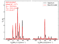
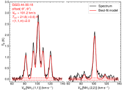
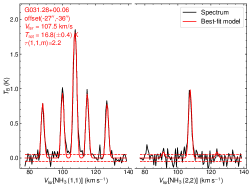
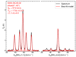
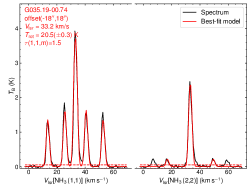
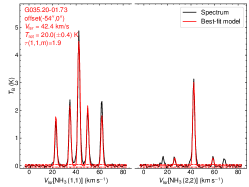
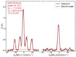
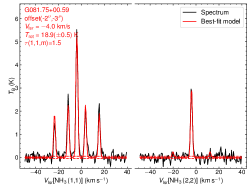
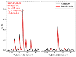
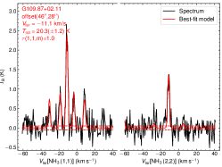
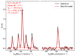
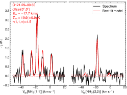
Figure A1: The observed spectra of NH₃(1,1) and NH₃(2,2) are in black, while the best fit from the code of Lu et al. (2015) is in red.

Appendix B The distribution of NH₃(1,1), NH₃(2,2) and ortho-NH₂D $1_{11}^{s}-1_{01}^{a}$

We present the spatial distribution maps NH₃(1,1), NH₃(2,2) and ortho-NH₂D $1_{11}^{s}-1_{01}^{a}$ in Figure B1-B12.

Figure B1: (a) The velocity-integrated intensity of the ortho-NH₂D $1_{11}^{s}-1_{01}^{a}$ contour (red contour) overlaid on the NH₃(1,1) main group velocity-integrated intensity image (gray scale and black contour) in G015.03-00.67. The contour levels start at 3$\sigma$ in steps of 2$\sigma$ for NH₂D $1_{11}^{s}-1_{01}^{a}$, while the contour levels start at 15$\sigma$ in steps of 36$\sigma$ for the NH₃(1,1) main group. The gray scale starts at 3$\sigma$. (b) The velocity-integrated intensity of the ortho-NH₂D $1_{11}^{s}-1_{01}^{a}$ contour (red contour) overlaid on the NH₃(2,2) main group velocity-integrated intensity image (Gray scale and black contour) in G015.03-00.67. The contour levels start at 3$\sigma$ in steps of 2$\sigma$ for the ortho-NH₂D $1_{11}^{s}-1_{01}^{a}$, while the contour levels start at 15$\sigma$ in steps of 24$\sigma$ for NH₃(2,2) main group. The gray scale starts at 3$\sigma$.

Figure B2: Same as Figure B1, but for source G023.44-00.18. (a) The red contour levels start at 5$\sigma$ in steps of 3$\sigma$, the black contour levels start at 30$\sigma$ in steps of 30$\sigma$, and the gray scale starts at 3$\sigma$. (b) The red contour levels start at 5$\sigma$ in steps of 3$\sigma$, the black contour levels start at 18$\sigma$ in steps of 18$\sigma$, and the gray scale starts at 3$\sigma$.

Figure B3: Same as Figure B1, but for source G031.28+00.06. (a) The red contour levels start at 3$\sigma$ in steps of 2$\sigma$, the black contour levels start at 24$\sigma$ in steps of 18$\sigma$, and the gray scale starts at 3$\sigma$. (b) The red contour levels start at 3$\sigma$ in steps of 2$\sigma$, the black contour levels start at 9$\sigma$ in steps of 9$\sigma$, and the gray scale starts at 3$\sigma$.

Figure B4: Same as Figure B1, but for source G034.39+00.22. (a) The red contour levels start at 5$\sigma$ in steps of 2$\sigma$, the black contour levels start at 42$\sigma$ in steps of 42$\sigma$, and the gray scale starts at 3$\sigma$. (b) The red contour levels start at 5$\sigma$ in steps of 2$\sigma$, the black contour levels start at 24$\sigma$ in steps of 24$\sigma$, and the gray scale starts at 3$\sigma$.

Figure B5: Same as Figure B1, but for source G035.19-00.74. (a) The red contour levels start at 5$\sigma$ in steps of 5$\sigma$, the black contour levels start at 90$\sigma$ in steps of 54$\sigma$, and the gray scale starts at 3$\sigma$. (b) The red contour levels start at 5$\sigma$ in steps of 5$\sigma$, the black contour levels start at 54$\sigma$ in steps of 27$\sigma$, and the gray scale starts at 3$\sigma$.

Figure B6: Same as Figure B1, but for source G035.20-01.73. (a) The red contour levels start at 5$\sigma$ in steps of 2$\sigma$, the black contour levels start at 24$\sigma$ in steps of 33$\sigma$, and the gray scale starts at 3$\sigma$. (b) The red contour levels start at 5$\sigma$ in steps of 2$\sigma$, the black contour levels start at 18$\sigma$ in steps of 24$\sigma$, and the gray scale starts at 3$\sigma$.

Figure B7: Same as Figure B1, but for source G075.76+00.33. (a) The red contour levels start at 3$\sigma$ in steps of 2$\sigma$, the black contour levels start at 48$\sigma$ in steps of 30$\sigma$, and the gray scale starts at 3$\sigma$. (b) The red contour levels start at 3$\sigma$ in steps of 2$\sigma$, the black contour levels start at 36$\sigma$ in steps of 15$\sigma$, and the gray scale starts at 3$\sigma$.

Figure B8: Same as Figure B1, but for source G081.75+00.59. (a) The red contour levels start at 36$\sigma$ in steps of 10$\sigma$, the black contour levels start at 9$\sigma$ in steps of 9$\sigma$, and the gray scale starts at 3$\sigma$. (b) The red contour levels start at 36$\sigma$ in steps of 10$\sigma$, the black contour levels start at 6$\sigma$ in steps of 9$\sigma$, and the gray scale starts at 3$\sigma$.

Figure B9: Same as Figure B1, but for source G081.87+00.78. (a) The red contour levels start at 3$\sigma$ in steps of 2$\sigma$, the black contour levels start at 15$\sigma$ in steps of 36$\sigma$, and the gray scale starts at 3$\sigma$. (b) The red contour levels start at 3$\sigma$ in steps of 2$\sigma$, the black contour levels start at 15$\sigma$ in steps of 24$\sigma$, and the gray scale starts at 3$\sigma$.

Figure B10: Same as Figure B1, but for source G109.87+02.11. (a) The red contour levels start at 5$\sigma$ in steps of 2$\sigma$, the black contour levels start at 6$\sigma$ in steps of 3$\sigma$, and the gray scale starts at 3$\sigma$. (b) The red contour levels start at 5$\sigma$ in steps of 2$\sigma$, the black contour levels start at 5$\sigma$ in steps of 3$\sigma$, and the gray scale starts at 3$\sigma$.

Figure B11: Same as Figure B1, but for source G111.54+00.77. (a) The red contour levels start at 3$\sigma$ in steps of 2$\sigma$, the black contour levels start at 12$\sigma$ in steps of 18$\sigma$, and the gray scale starts at 3$\sigma$. (b) The red contour levels start at 3$\sigma$ in steps of 2$\sigma$, the black contour levels start at 9$\sigma$ in steps of 12$\sigma$, and the gray scale starts at 3$\sigma$.

Figure B12: Same as Figure B1, but for source G121.29+00.65. (a) The red contour levels start at 7$\sigma$ in steps of 2$\sigma$, the black contour levels start at 7$\sigma$ in steps of 5$\sigma$, and the gray scale starts at 3$\sigma$. (b) The red contour levels start at 7$\sigma$ in steps of 2$\sigma$, the black contour levels start at 5$\sigma$ in steps of 3$\sigma$, and the gray scale starts at 3$\sigma$.

Appendix C Physical parameters of the calculation and the error

The rotation temperature $T_{\rm rot}$(2,2;1,1), colunm denstity of NH₃ and NH₂D, and deuterium fractionation are list in Table 1.

Table 1: Column density and deuterium fractionation

Source	Offset	$T_{\rm rot}$(2,2;1,1)	$N$(NH3)$\times$1015	$N$(NH2D)$\times$1013	$D_{\rm frac}$(NH3)$\times$100
	(arcsec, arcsec)	(K)	(cm-2)	(cm-2)
G015.03-00.67	(-9,-27)	24.8$\pm$0.7	2.0$\pm$0.2	1.2$\pm$0.1	0.59$\pm$0.09
	(-18,-18)	24.4$\pm$0.6	2.1$\pm$0.2	1.2$\pm$0.1	0.56$\pm$0.08
	(-27,-9)	24.1$\pm$0.5	1.7$\pm$0.1	1.1$\pm$0.1	0.7$\pm$0.1
	(-36,-18)	23.3$\pm$0.5	1.7$\pm$0.1	1.2$\pm$0.1	0.67$\pm$0.09
	(-45,-81)	21.6$\pm$0.9	1.7$\pm$0.1	0.9$\pm$0.1	0.51$\pm$0.08
	(-54,-108)	19.5$\pm$0.8	1.1$\pm$0.2	1.3$\pm$0.1	1.2$\pm$0.2
G023.44-00.18	(9,9)	20.6$\pm$0.6	0.46$\pm$0.04	1.2$\pm$0.1	2.5$\pm$0.3
	(-9,9)	20.8$\pm$0.6	0.70$\pm$0.05	1.5$\pm$0.1	2.1$\pm$0.2
	(9,-9)	21.6$\pm$0.5	0.79$\pm$0.07	2.0$\pm$0.1	2.6$\pm$0.3
	(-9,-9)	21.5$\pm$0.5	0.94$\pm$0.07	2.6$\pm$0.1	2.8$\pm$0.2
	(-27,-9)	20.4$\pm$0.6	1.02$\pm$0.05	1.4$\pm$0.1	1.3$\pm$0.1
	(0,-27)	21.2$\pm$0.5	0.80$\pm$0.07	1.8$\pm$0.1	2.3$\pm$0.2
	(-18,-27)	20.3$\pm$0.5	0.67$\pm$0.06	1.8$\pm$0.1	2.7$\pm$0.3
	(-36,-27)	17.8$\pm$0.7	1.29$\pm$0.09	1.1$\pm$0.1	0.9$\pm$0.1
	(-27,36)	14.8$\pm$0.7	0.31$\pm$0.05	0.9$\pm$0.1	3.1$\pm$0.6
G031.28+00.06	(18,18)	21.7$\pm$0.5	0.69$\pm$0.08	0.81$\pm$0.09	0.07$\pm$0.01
	(9,18)	22.1$\pm$0.5	0.9$\pm$0.1	0.81$\pm$0.09	0.062$\pm$0.008
	(-18,-18)	20.3$\pm$0.5	0.9$\pm$0.1	0.87$\pm$0.09	0.08$\pm$0.01
	(-18,-27)	18.9$\pm$0.5	0.8$\pm$0.1	0.94$\pm$0.09	0.11$\pm$0.01
	(-18,-36)	17.6$\pm$0.4	0.7$\pm$0.1	0.94$\pm$0.08	0.12$\pm$0.01
	(-18,-45)	16.7$\pm$0.5	0.63$\pm$0.08	0.84$\pm$0.09	0.12$\pm$0.02
	(-27,-18)	19.5$\pm$0.5	0.8$\pm$0.1	0.87$\pm$0.09	0.09$\pm$0.01
	(-27,-27)	18.2$\pm$0.5	0.8$\pm$0.1	0.96$\pm$0.09	0.11$\pm$0.01
	(-27,-36)	17.1$\pm$0.4	0.8$\pm$0.1	0.96$\pm$0.08	0.12$\pm$0.01
	(-27,-45)	16.4$\pm$0.4	0.70$\pm$0.09	0.94$\pm$0.09	0.13$\pm$0.02
G034.39+00.22	(-9,45)	19.5$\pm$0.4	2.1$\pm$0.2	3.5$\pm$0.2	1.7$\pm$0.2
	(-9,36)	20.0$\pm$0.4	2.2$\pm$0.2	4.2$\pm$0.2	1.9$\pm$0.2
	(-9,27)	20.2$\pm$0.4	2.2$\pm$0.2	4.9$\pm$0.2	2.2$\pm$0.2
	(-9,18)	20.2$\pm$0.4	2.2$\pm$0.2	5.1$\pm$0.2	2.3$\pm$0.2
	(-9,9)	20.1$\pm$0.4	2.1$\pm$0.2	4.9$\pm$0.2	2.3$\pm$0.2
	(-9,0)	20.0$\pm$0.3	2.1$\pm$0.2	4.7$\pm$0.1	2.2$\pm$0.2
	(-9,-9)	19.9$\pm$0.3	2.0$\pm$0.2	4.8$\pm$0.1	2.4$\pm$0.2
	(-9,-18)	19.6$\pm$0.3	2.0$\pm$0.2	5.4$\pm$0.2	2.7$\pm$0.2
	(-9,-27)	19.2$\pm$0.3	1.9$\pm$0.2	6.0$\pm$0.2	3.1$\pm$0.3
	(-9,-36)	18.7$\pm$0.3	1.8$\pm$0.1	6.1$\pm$0.2	3.4$\pm$0.3
	(-9,-45)	18.1$\pm$0.3	1.6$\pm$0.1	5.6$\pm$0.2	3.5$\pm$0.3
G035.19-00.74	(-45,45)	15.8$\pm$0.3	0.78$\pm$0.07	3.1$\pm$0.1	4.0$\pm$0.4
	(-36,36)	17.1$\pm$0.3	0.91$\pm$0.09	3.4$\pm$0.1	3.7$\pm$0.4
	(-27,27)	18.9$\pm$0.4	1.1$\pm$0.1	3.7$\pm$0.1	3.3$\pm$0.3
	(-18,18)	20.5$\pm$0.3	1.4$\pm$0.1	3.6$\pm$0.1	2.6$\pm$0.2
	(-9,9)	21.7$\pm$0.3	1.5$\pm$0.1	2.9$\pm$0.1	2.0$\pm$0.2
	(0,0)	22.1$\pm$0.3	1.4$\pm$0.1	2.3$\pm$0.1	1.7$\pm$0.2
	(9,-9)	21.7$\pm$0.3	1.2$\pm$0.1	1.92$\pm$0.09	1.6$\pm$0.1
	(18,-18)	20.6$\pm$0.3	1.02$\pm$0.09	1.80$\pm$0.09	1.8$\pm$0.2
	(27,-27)	18.9$\pm$0.4	0.80$\pm$0.07	1.7$\pm$0.1	2.1$\pm$0.2
	(36,-36)	16.7$\pm$0.5	0.71$\pm$0.06	1.8$\pm$0.1	2.5$\pm$0.3
	(45,-45)	14.5$\pm$0.6	0.85$\pm$0.09	1.8$\pm$0.1	2.1$\pm$0.3
G035.20-01.73	(-18,0)	22.4$\pm$0.6	0.65$\pm$0.08	2.0$\pm$0.1	3.0$\pm$0.4
	(-27,0)	21.6$\pm$0.5	0.89$\pm$0.09	2.5$\pm$0.1	2.8$\pm$0.3
	(-36,0)	21.0$\pm$0.4	1.1$\pm$0.1	3.4$\pm$0.1	3.0$\pm$0.3
	(-45,0)	20.4$\pm$0.4	1.3$\pm$0.1	4.3$\pm$0.1	3.2$\pm$0.3
	(-54,0)	19.7$\pm$0.4	1.4$\pm$0.1	4.9$\pm$0.1	3.4$\pm$0.4
	(-63,0)	19.0$\pm$0.3	1.3$\pm$0.1	4.6$\pm$0.1	3.5$\pm$0.4
	(-72,0)	18.3$\pm$0.3	1.1$\pm$0.1	3.7$\pm$0.1	3.4$\pm$0.3
	(-54,18)	19.7$\pm$0.4	0.75$\pm$0.07	3.1$\pm$0.1	4.1$\pm$0.4
	(-54,-18)	20.0$\pm$0.4	1.0$\pm$0.1	2.4$\pm$0.1	2.4$\pm$0.3
G075.76+00.33	(0,-27)	22.9$\pm$0.2	0.54$\pm$0.04	1.2$\pm$0.1	2.3$\pm$0.3
	(-9,-27)	22.7$\pm$0.2	0.62$\pm$0.04	1.4$\pm$0.1	2.2$\pm$0.2
	(-18,-27)	22.3$\pm$0.2	0.68$\pm$0.05	1.4$\pm$0.1	2.0$\pm$0.2
	(-27,-27)	21.9$\pm$0.3	0.69$\pm$0.05	1.3$\pm$0.1	1.8$\pm$0.2
	(-36,-27)	21.4$\pm$0.3	0.66$\pm$0.05	1.2$\pm$0.1	1.8$\pm$0.2
	(-45,-27)	21.1$\pm$0.4	0.57$\pm$0.04	1.1$\pm$0.1	2.0$\pm$0.3
G081.75+00.59	(17,46)	18.1$\pm$0.4	1.5$\pm$0.2	6.1$\pm$0.2	4.0$\pm$0.4
	(3,46)	18.2$\pm$0.4	1.6$\pm$0.2	6.7$\pm$0.2	4.2$\pm$0.4
	(-11,46)	18.6$\pm$0.4	1.3$\pm$0.1	5.5$\pm$0.1	4.3$\pm$0.4
	(17,32)	18.1$\pm$0.4	1.5$\pm$0.2	6.5$\pm$0.2	4.3$\pm$0.4
	(3,32)	18.3$\pm$0.3	1.7$\pm$0.2	7.1$\pm$0.2	4.2$\pm$0.4
	(-11,32)	18.6$\pm$0.3	1.5$\pm$0.1	6.1$\pm$0.1	4.1$\pm$0.4
	(17,18)	18.6$\pm$0.4	1.4$\pm$0.1	6.9$\pm$0.2	4.8$\pm$0.5
	(3,18)	18.7$\pm$0.3	1.7$\pm$0.2	7.6$\pm$0.2	4.4$\pm$0.4
	(-11,18)	19.1$\pm$0.3	1.6$\pm$0.1	6.9$\pm$0.1	4.3$\pm$0.4
	(17,4)	19.1$\pm$0.4	1.2$\pm$0.1	6.7$\pm$0.2	5.6$\pm$0.6
	(3,4)	19.0$\pm$0.4	1.5$\pm$0.1	7.7$\pm$0.2	5.0$\pm$0.5
	(-11,4)	19.3$\pm$0.4	1.6$\pm$0.1	7.3$\pm$0.2	4.7$\pm$0.4
	(17,-10)	18.9$\pm$0.4	0.93$\pm$0.09	5.7$\pm$0.2	6.2$\pm$0.6
	(3,-10)	19.1$\pm$0.4	1.2$\pm$0.1	6.9$\pm$0.2	5.8$\pm$0.6
	(-11,-10)	19.3$\pm$0.4	1.3$\pm$0.1	6.8$\pm$0.2	5.3$\pm$0.5
	(17,-24)	19.6$\pm$0.5	0.57$\pm$0.06	3.9$\pm$0.1	6.8$\pm$0.8
	(3,-24)	19.6$\pm$0.5	0.77$\pm$0.08	5.0$\pm$0.1	6.5$\pm$0.7
	(-11,-24)	19.7$\pm$0.4	0.97$\pm$0.09	5.4$\pm$0.1	5.6$\pm$0.6
	(-23,-11)	19.2$\pm$0.4	1.3$\pm$0.1	6.0$\pm$0.1	4.4$\pm$0.4
	(-37,-11)	18.4$\pm$0.3	1.4$\pm$0.1	4.8$\pm$0.1	3.4$\pm$0.3
	(-51,-11)	18.0$\pm$0.4	1.3$\pm$0.1	3.7$\pm$0.1	2.8$\pm$0.3
	(-23,-25)	19.6$\pm$0.4	1.2$\pm$0.1	5.4$\pm$0.1	4.7$\pm$0.4
	(-37,-25)	18.6$\pm$0.3	1.5$\pm$0.1	4.9$\pm$0.1	3.4$\pm$0.3
	(-51,-25)	18.0$\pm$0.4	1.5$\pm$0.1	4.0$\pm$0.1	2.6$\pm$0.3
	(-23,-39)	19.9$\pm$0.4	1.1$\pm$0.1	4.8$\pm$0.1	4.4$\pm$0.4
	(-37,-39)	19.1$\pm$0.4	1.4$\pm$0.1	4.8$\pm$0.1	3.4$\pm$0.3
	(-51,-39)	18.3$\pm$0.4	1.5$\pm$0.1	3.7$\pm$0.1	2.6$\pm$0.3
	(-23,-53)	19.1$\pm$0.4	1.3$\pm$0.1	4.6$\pm$0.1	3.6$\pm$0.4
	(-37,-53)	19.2$\pm$0.3	1.5$\pm$0.1	4.7$\pm$0.1	3.0$\pm$0.3
	(-51,-53)	18.7$\pm$0.4	1.5$\pm$0.1	3.6$\pm$0.1	2.4$\pm$0.2
	(-23,-67)	19.3$\pm$0.4	1.4$\pm$0.1	5.1$\pm$0.1	3.5$\pm$0.3
	(-37,-67)	19.5$\pm$0.3	1.8$\pm$0.2	5.2$\pm$0.1	3.0$\pm$0.3
	(-51,-67)	19.2$\pm$0.4	1.7$\pm$0.2	3.9$\pm$0.1	2.3$\pm$0.2
	(-23,-81)	20.6$\pm$0.5	1.4$\pm$0.1	5.6$\pm$0.2	4.1$\pm$0.4
	(-37,-81)	20.1$\pm$0.4	1.8$\pm$0.2	5.9$\pm$0.2	3.4$\pm$0.4
	(-51,-81)	19.8$\pm$0.5	1.7$\pm$0.2	4.6$\pm$0.1	2.7$\pm$0.3
	(-23,-95)	21.9$\pm$0.6	1.3$\pm$0.1	5.6$\pm$0.2	4.4$\pm$0.5
	(-37,-95)	21.0$\pm$0.6	1.6$\pm$0.2	6.2$\pm$0.2	3.8$\pm$0.4
	(-51,-95)	20.1$\pm$0.6	1.7$\pm$0.2	4.9$\pm$0.2	2.9$\pm$0.3
	(-23,-109)	23.0$\pm$0.6	1.4$\pm$0.1	5.2$\pm$0.2	3.6$\pm$0.4
	(-37,-109)	21.9$\pm$0.7	1.7$\pm$0.2	5.8$\pm$0.2	3.5$\pm$0.4
	(-51,-109)	20.5$\pm$0.8	1.7$\pm$0.2	4.6$\pm$0.2	2.7$\pm$0.3
	(-23,-123)	23.9$\pm$0.6	1.7$\pm$0.2	5.1$\pm$0.2	3.0$\pm$0.4
	(-37,-123)	22.8$\pm$0.7	2.4$\pm$0.2	5.4$\pm$0.2	2.2$\pm$0.2
	(-51,-123)	21.6$\pm$0.8	1.5$\pm$0.2	4.1$\pm$0.2	2.8$\pm$0.4
G081.87+00.78	(45,-18)	20.2$\pm$0.3	0.25$\pm$0.02	1.7$\pm$0.1	6.8$\pm$0.7
	(45,-9)	20.2$\pm$0.3	0.30$\pm$0.02	2.1$\pm$0.1	6.8$\pm$0.6
	(45,0)	20.5$\pm$0.3	0.30$\pm$0.02	2.2$\pm$0.1	7.2$\pm$0.6
	(45,9)	20.7$\pm$0.4	0.25$\pm$0.02	2.2$\pm$0.1	8.6$\pm$0.7
	(36,9)	22.1$\pm$0.4	0.31$\pm$0.02	2.1$\pm$0.1	6.8$\pm$0.6
	(27,18)	23.3$\pm$0.4	0.30$\pm$0.02	1.8$\pm$0.1	6.1$\pm$0.6
	(18,18)	24.2$\pm$0.4	0.43$\pm$0.03	2.2$\pm$0.1	5.1$\pm$0.4
	(9,18)	25.0$\pm$0.4	0.60$\pm$0.04	2.7$\pm$0.1	4.5$\pm$0.4
	(0,18)	25.6$\pm$0.4	0.76$\pm$0.05	2.7$\pm$0.1	3.6$\pm$0.3
G109.87+02.11	(95,45)	21.6$\pm$1.3	0.3$\pm$0.1	1.19$\pm$0.09	3.8$\pm$1.5
	(81,31)	21.4$\pm$0.8	0.44$\pm$0.06	1.80$\pm$0.09	4.1$\pm$0.6
	(67,17)	21.9$\pm$0.8	0.51$\pm$0.06	2.0$\pm$0.1	3.9$\pm$0.5
	(53,3)	22.5$\pm$1.0	0.51$\pm$0.08	1.7$\pm$0.1	3.3$\pm$0.5
	(39,-11)	21.2$\pm$1.1	0.6$\pm$0.1	1.02$\pm$0.09	1.6$\pm$0.3
	(81,45)	21.8$\pm$1.3	0.3$\pm$0.1	1.6$\pm$0.1	5.5$\pm$2.4
	(67,31)	21.2$\pm$0.9	0.51$\pm$0.06	2.0$\pm$0.1	4.0$\pm$0.5
	(53,17)	21.2$\pm$0.9	0.61$\pm$0.08	2.1$\pm$0.1	3.4$\pm$0.5
	(39,3)	22.1$\pm$1.0	0.56$\pm$0.08	1.6$\pm$0.1	2.9$\pm$0.5
	(25,-11)	23.1$\pm$0.9	0.57$\pm$0.08	0.86$\pm$0.09	1.5$\pm$0.3
	(-3,30)	21.7$\pm$1.0	0.45$\pm$0.07	0.62$\pm$0.08	1.4$\pm$0.3
	(-3,16)	23.3$\pm$1.0	0.42$\pm$0.06	0.64$\pm$0.08	1.5$\pm$0.3
	(-17,-21)	24.6$\pm$0.8	0.58$\pm$0.07	0.6$\pm$0.1	1.1$\pm$0.2
G111.54+00.77	(45,-81)	21.3$\pm$0.3	0.75$\pm$0.07	1.5$\pm$0.1	2.0$\pm$0.2
	(36,-81)	21.5$\pm$0.2	0.84$\pm$0.07	1.6$\pm$0.1	1.9$\pm$0.2
	(27,-81)	22.1$\pm$0.2	0.89$\pm$0.08	1.7$\pm$0.1	1.9$\pm$0.2
	(18,-81)	22.9$\pm$0.2	0.93$\pm$0.08	1.7$\pm$0.1	1.8$\pm$0.2
	(9,-81)	23.5$\pm$0.2	1.02$\pm$0.09	1.6$\pm$0.1	1.6$\pm$0.2
	(0,-81)	23.9$\pm$0.3	1.1$\pm$0.1	1.5$\pm$0.1	1.4$\pm$0.2
	(-9,-81)	24.7$\pm$0.3	0.94$\pm$0.08	1.4$\pm$0.1	1.5$\pm$0.2
	(-18,-81)	24.9$\pm$0.4	0.74$\pm$0.07	1.3$\pm$0.1	1.8$\pm$0.2
	(-27,-81)	24.2$\pm$0.4	0.56$\pm$0.05	1.5$\pm$0.2	2.7$\pm$0.4
	(-36,-81)	22.6$\pm$0.4	0.46$\pm$0.04	1.3$\pm$0.1	2.8$\pm$0.4
	(-45,-45)	21.9$\pm$0.5	0.27$\pm$0.03	1.2$\pm$0.1	4.3$\pm$0.6
	(-45,-54)	21.8$\pm$0.5	0.29$\pm$0.03	1.1$\pm$0.1	3.9$\pm$0.6
	(-45,-63)	21.6$\pm$0.5	0.33$\pm$0.03	1.0$\pm$0.1	2.9$\pm$0.5
	(-45,-72)	21.4$\pm$0.4	0.34$\pm$0.03	0.9$\pm$0.1	2.8$\pm$0.5
	(-45,-99)	21.0$\pm$0.5	0.49$\pm$0.06	2.2$\pm$0.1	4.4$\pm$0.6
	(-45,-108)	20.3$\pm$0.5	0.52$\pm$0.06	2.4$\pm$0.1	4.6$\pm$0.6
	(-45,-117)	20.0$\pm$0.5	0.47$\pm$0.05	2.3$\pm$0.1	4.9$\pm$0.6
	(-45,-126)	20.1$\pm$0.6	0.36$\pm$0.04	2.0$\pm$0.1	5.6$\pm$0.7
	(-45,-135)	21.1$\pm$0.7	0.22$\pm$0.03	1.5$\pm$0.1	6.7$\pm$1.0
	(-18,-18)	26.5$\pm$0.5	0.33$\pm$0.02	1.3$\pm$0.2	3.9$\pm$0.6
G121.29+00.65	(49,-49)	13.6$\pm$1.4	0.4$\pm$0.1	1.3$\pm$0.3	3.6$\pm$1.2
	(35,-35)	15.4$\pm$0.8	0.51$\pm$0.09	1.7$\pm$0.2	3.3$\pm$0.7
	(21,-21)	17.3$\pm$0.6	0.77$\pm$0.09	2.0$\pm$0.1	2.5$\pm$0.3
	(7,-7)	19.0$\pm$0.6	0.9$\pm$0.1	2.1$\pm$0.2	2.2$\pm$0.3
	(-7,7)	18.6$\pm$0.6	0.9$\pm$0.1	2.0$\pm$0.2	2.2$\pm$0.3
	(-21,21)	16.9$\pm$0.7	0.7$\pm$0.1	1.5$\pm$0.1	2.3$\pm$0.4
	(-35,35)	16.3$\pm$1.2	0.27$\pm$0.06	1.1$\pm$0.2	3.9$\pm$1.1
	(49,-30)	16.1$\pm$0.9	0.48$\pm$0.08	1.5$\pm$0.2	3.1$\pm$0.6
	(35,-16)	17.1$\pm$0.6	0.71$\pm$0.09	1.8$\pm$0.1	2.6$\pm$0.4
	(21,-2)	18.2$\pm$0.5	0.9$\pm$0.1	1.9$\pm$0.1	2.2$\pm$0.3
	(7,12)	18.5$\pm$0.6	0.9$\pm$0.1	1.9$\pm$0.2	2.1$\pm$0.3
	(-7,26)	17.3$\pm$0.8	0.6$\pm$0.1	1.4$\pm$0.1	2.4$\pm$0.4
	(-21,40)	15.9$\pm$1.1	0.36$\pm$0.08	0.9$\pm$0.2	2.6$\pm$0.7
	(30,-49)	13.8$\pm$1.4	0.32$\pm$0.09	1.3$\pm$0.2	4.1$\pm$1.4
	(16,-35)	15.0$\pm$0.8	0.6$\pm$0.1	1.6$\pm$0.2	2.7$\pm$0.5
	(2,-21)	18.2$\pm$0.6	0.7$\pm$0.1	1.9$\pm$0.1	2.7$\pm$0.4
	(-12,-7)	18.9$\pm$0.6	1.0$\pm$0.1	2.0$\pm$0.2	2.0$\pm$0.3
	(-26,7)	17.5$\pm$0.5	0.9$\pm$0.1	1.8$\pm$0.1	2.0$\pm$0.3
	(-40,21)	16.0$\pm$0.6	0.72$\pm$0.09	1.5$\pm$0.1	2.0$\pm$0.3
	(-54,35)	16.2$\pm$1.2	0.32$\pm$0.07	1.1$\pm$0.2	3.4$\pm$1.0

Appendix D The method of pixel averaging In Each Source

The method of pixel averaging for each source is shown in Figure D1.

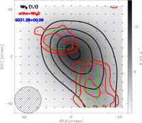
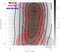
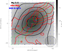
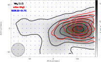
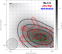
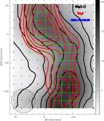
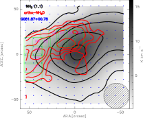
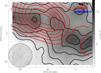
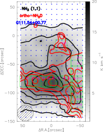
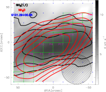
Figure D1: The pixels in the box are the average area. Within each source, the order of the region numbers is the order in Table 1.

Appendix E The relationship between deuterium fractionation of NH₃ and distance of NH₃ Peak

The relationship between deuterium fractionation of NH₃ and distance of NH₃ peak are shown in Figure E1. The relationship between rotation temperature of NH₃ and distance of NH₃ peak are shown in Figure E2.

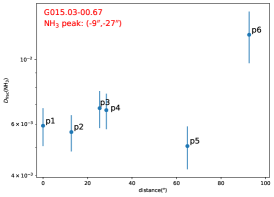
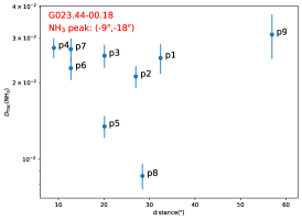
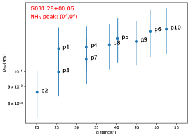
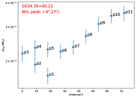
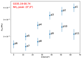
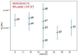
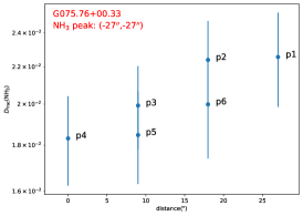
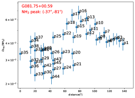
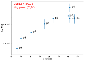
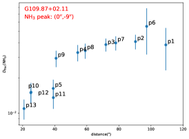
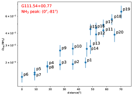
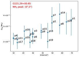
Figure E1: The relationship between deuterium fractionation of NH₃ and distance of NH₃ peak.

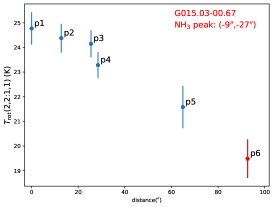
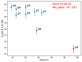
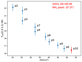
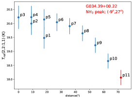
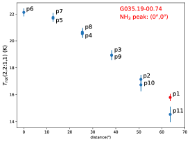
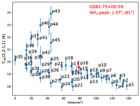
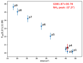
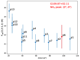
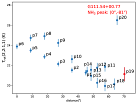
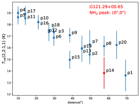
Figure E2: The relationship between rotation temperature of NH₃ and distance of NH₃ peak. The red marker is the position with the highest deuterium fractionation of NH₃.

References

- Beuther et al. (2022) Beuther, H., Schneider, N., Simon, R., et al. 2022, A&A, 659, A77, doi: 10.1051/0004-6361/202142689
- Busquet et al. (2010) Busquet, G., Palau, A., Estalella, R., et al. 2010, A&A, 517, L6, doi: 10.1051/0004-6361/201014866
- Caselli (2002) Caselli, P. 2002, Planet. Space Sci., 50, 1133, doi: 10.1016/S0032-0633(02)00074-0
- Caselli & Ceccarelli (2012) Caselli, P., & Ceccarelli, C. 2012, A&A Rev., 20, 56, doi: 10.1007/s00159-012-0056-x
- Caselli et al. (2008) Caselli, P., Vastel, C., Ceccarelli, C., et al. 2008, A&A, 492, 703, doi: 10.1051/0004-6361:20079009
- Caselli et al. (1998) Caselli, P., Walmsley, C. M., Terzieva, R., & Herbst, E. 1998, ApJ, 499, 234, doi: 10.1086/305624
- Ceccarelli et al. (2014) Ceccarelli, C., Caselli, P., Bockelée-Morvan, D., et al. 2014, in Protostars and Planets VI, ed. H. Beuther, R. S. Klessen, C. P. Dullemond, & T. Henning, 859–882, doi: 10.2458/azu_uapress_9780816531240-ch037
- Christensen et al. (2023) Christensen, I. B., Wyrowski, F., Menten, K. M., Beuther, H., & Cascade Team. 2023, in Physics and Chemistry of Star Formation: The Dynamical ISM Across Time and Spatial Scales, 253
- Crapsi et al. (2005) Crapsi, A., Caselli, P., Walmsley, C. M., et al. 2005, ApJ, 619, 379, doi: 10.1086/426472
- Crapsi et al. (2007) Crapsi, A., Caselli, P., Walmsley, M. C., & Tafalla, M. 2007, A&A, 470, 221, doi: 10.1051/0004-6361:20077613
- Dent et al. (1984) Dent, W. R. F., Little, L. T., & White, G. J. 1984, MNRAS, 210, 173, doi: 10.1093/mnras/210.1.173
- Dickel et al. (1978) Dickel, J. R., Dickel, H. R., & Wilson, W. J. 1978, ApJ, 223, 840, doi: 10.1086/156317
- Emprechtinger et al. (2009) Emprechtinger, M., Caselli, P., Volgenau, N. H., Stutzki, J., & Wiedner, M. C. 2009, A&A, 493, 89, doi: 10.1051/0004-6361:200810324
- Fallscheer et al. (2013) Fallscheer, C., Reid, M. A., Di Francesco, J., et al. 2013, ApJ, 773, 102, doi: 10.1088/0004-637X/773/2/102
- Fey et al. (1992) Fey, A. L., Claussen, M. J., Gaume, R. A., Nedoluha, G. E., & Johnston, K. J. 1992, AJ, 103, 234, doi: 10.1086/116056
- Fontani et al. (2015) Fontani, F., Busquet, G., Palau, A., et al. 2015, A&A, 575, A87, doi: 10.1051/0004-6361/201424753
- Fontani et al. (2011) Fontani, F., Palau, A., Caselli, P., et al. 2011, A&A, 529, L7, doi: 10.1051/0004-6361/201116631
- Gibb et al. (2003) Gibb, A. G., Hoare, M. G., Little, L. T., & Wright, M. C. H. 2003, MNRAS, 339, 1011, doi: 10.1046/j.1365-8711.2003.06251.x
- Goldsmith & Langer (1999) Goldsmith, P. F., & Langer, W. D. 1999, ApJ, 517, 209, doi: 10.1086/307195
- Harvey et al. (1986) Harvey, P. M., Joy, M., Lester, D. F., & Wilking, B. A. 1986, ApJ, 300, 737, doi: 10.1086/163848
- Hennemann et al. (2012) Hennemann, M., Motte, F., Schneider, N., et al. 2012, A&A, 543, L3, doi: 10.1051/0004-6361/201219429
- Herbst (1982) Herbst, E. 1982, A&A, 111, 76
- Ho & Townes (1983) Ho, P. T. P., & Townes, C. H. 1983, ARA&A, 21, 239, doi: 10.1146/annurev.aa.21.090183.001323
- Hogge et al. (2018) Hogge, T., Jackson, J., Stephens, I., et al. 2018, ApJS, 237, 27, doi: 10.3847/1538-4365/aacf94
- Hsu et al. (2021) Hsu, C.-J., Tan, J. C., Goodson, M. D., et al. 2021, MNRAS, 502, 1104, doi: 10.1093/mnras/staa4031
- Hughes & Wouterloot (1984) Hughes, V. A., & Wouterloot, J. G. A. 1984, ApJ, 276, 204, doi: 10.1086/161603
- Jensen et al. (2021) Jensen, S. S., Jørgensen, J. K., Kristensen, L. E., et al. 2021, A&A, 650, A172, doi: 10.1051/0004-6361/202140560
- Juárez et al. (2019) Juárez, C., Liu, H. B., Girart, J. M., et al. 2019, A&A, 621, A140, doi: 10.1051/0004-6361/201834173
- Keown et al. (2019) Keown, J., Di Francesco, J., Rosolowsky, E., et al. 2019, ApJ, 884, 4, doi: 10.3847/1538-4357/ab3e76
- Kirby (2009) Kirby, L. 2009, ApJ, 694, 1056, doi: 10.1088/0004-637X/694/2/1056
- Kurtz et al. (2000) Kurtz, S., Cesaroni, R., Churchwell, E., Hofner, P., & Walmsley, C. M. 2000, in Protostars and Planets IV, ed. V. Mannings, A. P. Boss, & S. S. Russell, 299–326
- Lada (1976) Lada, C. J. 1976, ApJS, 32, 603, doi: 10.1086/190409
- Lada et al. (1991) Lada, E. A., Bally, J., & Stark, A. A. 1991, ApJ, 368, 432, doi: 10.1086/169708
- Li et al. (2017) Li, S., Wang, J., Zhang, Z.-Y., et al. 2017, MNRAS, 466, 248, doi: 10.1093/mnras/stw3076
- Li et al. (2021) Li, S., Lu, X., Zhang, Q., et al. 2021, ApJ, 912, L7, doi: 10.3847/2041-8213/abf64f
- Li et al. (2024) Li, Y., Wang, J., Li, J., et al. 2024, MNRAS, 527, 5049, doi: 10.1093/mnras/stad3480
- Linsky et al. (1995) Linsky, J. L., Diplas, A., Wood, B. E., et al. 1995, ApJ, 451, 335, doi: 10.1086/176223
- Lis et al. (2002) Lis, D. C., Gerin, M., Phillips, T. G., & Motte, F. 2002, ApJ, 569, 322, doi: 10.1086/339232
- Little et al. (1985) Little, L. T., Dent, W. R. F., Heaton, B., Davies, S. R., & White, G. J. 1985, MNRAS, 217, 227, doi: 10.1093/mnras/217.2.227
- Lu et al. (2015) Lu, X., Zhang, Q., Wang, K., & Gu, Q. 2015, ApJ, 805, 171, doi: 10.1088/0004-637X/805/2/171
- Luisi et al. (2016) Luisi, M., Anderson, L. D., Balser, D. S., Bania, T. M., & Wenger, T. V. 2016, ApJ, 824, 125, doi: 10.3847/0004-637X/824/2/125
- Majumdar et al. (2017) Majumdar, L., Gratier, P., Ruaud, M., et al. 2017, MNRAS, 466, 4470, doi: 10.1093/mnras/stw3360
- Mangum et al. (1991) Mangum, J. G., Wootten, A., & Mundy, L. G. 1991, ApJ, 378, 576, doi: 10.1086/170459
- Mangum et al. (1992) —. 1992, ApJ, 388, 467, doi: 10.1086/171167
- Matthews et al. (1973) Matthews, H. E., Goss, W. M., Winnberg, A., & Habing, H. J. 1973, A&A, 29, 309
- Miralles et al. (1994) Miralles, M. P., Rodriguez, L. F., & Scalise, E. 1994, ApJS, 92, 173, doi: 10.1086/191965
- Motte et al. (2007) Motte, F., Bontemps, S., Schilke, P., et al. 2007, A&A, 476, 1243, doi: 10.1051/0004-6361:20077843
- Müller et al. (2005) Müller, H. S. P., Schlöder, F., Stutzki, J., & Winnewisser, G. 2005, Journal of Molecular Structure, 742, 215, doi: 10.1016/j.molstruc.2005.01.027
- Müller et al. (2001) Müller, H. S. P., Thorwirth, S., Roth, D. A., & Winnewisser, G. 2001, A&A, 370, L49, doi: 10.1051/0004-6361:20010367
- Neill et al. (2013) Neill, J. L., Crockett, N. R., Bergin, E. A., Pearson, J. C., & Xu, L.-H. 2013, ApJ, 777, 85, doi: 10.1088/0004-637X/777/2/85
- Nguyen Luong et al. (2011) Nguyen Luong, Q., Motte, F., Schuller, F., et al. 2011, A&A, 529, A41, doi: 10.1051/0004-6361/201016271
- Öberg et al. (2021) Öberg, K. I., Cleeves, L. I., Bergner, J. B., et al. 2021, AJ, 161, 38, doi: 10.3847/1538-3881/abc74d
- Oliveira et al. (2003) Oliveira, C. M., Hébrard, G., Howk, J. C., et al. 2003, ApJ, 587, 235, doi: 10.1086/368019
- Pagani et al. (1992) Pagani, L., Salez, M., & Wannier, P. G. 1992, A&A, 258, 479
- Pazukhin et al. (2023) Pazukhin, A. G., Zinchenko, I. I., Trofimova, E. A., Henkel, C., & Semenov, D. A. 2023, MNRAS, 526, 3673, doi: 10.1093/mnras/stad2976
- Persi et al. (2006) Persi, P., Tapia, M., & Smith, H. A. 2006, A&A, 445, 971, doi: 10.1051/0004-6361:20053251
- Pillai et al. (2011) Pillai, T., Kauffmann, J., Wyrowski, F., et al. 2011, A&A, 530, A118, doi: 10.1051/0004-6361/201015899
- Pillai et al. (2007) Pillai, T., Wyrowski, F., Hatchell, J., Gibb, A. G., & Thompson, M. A. 2007, A&A, 467, 207, doi: 10.1051/0004-6361:20065682
- Povich et al. (2009) Povich, M. S., Churchwell, E., Bieging, J. H., et al. 2009, ApJ, 696, 1278, doi: 10.1088/0004-637X/696/2/1278
- Rathborne et al. (2006) Rathborne, J. M., Jackson, J. M., & Simon, R. 2006, ApJ, 641, 389, doi: 10.1086/500423
- Reboussin et al. (2014) Reboussin, L., Wakelam, V., Guilloteau, S., & Hersant, F. 2014, MNRAS, 440, 3557, doi: 10.1093/mnras/stu462
- Reid & Wilson (2005) Reid, M. A., & Wilson, C. D. 2005, ApJ, 625, 891, doi: 10.1086/429790
- Ren et al. (2011) Ren, J. Z., Liu, T., Wu, Y., & Li, L. 2011, MNRAS, 415, L49, doi: 10.1111/j.1745-3933.2011.01076.x
- Rodgers & Charnley (2001) Rodgers, S. D., & Charnley, S. B. 2001, ApJ, 553, 613, doi: 10.1086/320987
- Rodriguez Kuiper et al. (1978) Rodriguez Kuiper, E. N., Zuckerman, B., & Kuiper, T. B. H. 1978, ApJ, 219, L49, doi: 10.1086/182604
- Roshi et al. (2005) Roshi, D. A., Goss, W. M., Anantharamaiah, K. R., & Jeyakumar, S. 2005, ApJ, 626, 253, doi: 10.1086/429747
- Roueff et al. (2005) Roueff, E., Lis, D. C., van der Tak, F. F. S., Gerin, M., & Goldsmith, P. F. 2005, A&A, 438, 585, doi: 10.1051/0004-6361:20052724
- Ruaud et al. (2015) Ruaud, M., Loison, J. C., Hickson, K. M., et al. 2015, MNRAS, 447, 4004, doi: 10.1093/mnras/stu2709
- Rygl et al. (2010) Rygl, K. L. J., Brunthaler, A., Reid, M. J., et al. 2010, A&A, 511, A2, doi: 10.1051/0004-6361/200913135
- Rygl et al. (2014) Rygl, K. L. J., Goedhart, S., Polychroni, D., et al. 2014, MNRAS, 440, 427, doi: 10.1093/mnras/stu300
- Saito et al. (2000) Saito, S., Ozeki, H., Ohishi, M., & Yamamoto, S. 2000, ApJ, 535, 227, doi: 10.1086/308818
- Sakai et al. (2012) Sakai, T., Sakai, N., Furuya, K., et al. 2012, ApJ, 747, 140, doi: 10.1088/0004-637X/747/2/140
- Sharma et al. (2017) Sharma, S., Pandey, A. K., Ojha, D. K., et al. 2017, MNRAS, 467, 2943, doi: 10.1093/mnras/stx014
- Shepherd et al. (2004) Shepherd, D. S., Kurtz, S. E., & Testi, L. 2004, ApJ, 601, 952, doi: 10.1086/380633
- Shepherd et al. (2003) Shepherd, D. S., Testi, L., & Stark, D. P. 2003, ApJ, 584, 882, doi: 10.1086/345743
- Sipilä et al. (2013) Sipilä, O., Caselli, P., & Harju, J. 2013, A&A, 554, A92, doi: 10.1051/0004-6361/201220922
- Sipilä et al. (2015a) —. 2015a, A&A, 578, A55, doi: 10.1051/0004-6361/201424364
- Sipilä et al. (2015b) Sipilä, O., Harju, J., Caselli, P., & Schlemmer, S. 2015b, A&A, 581, A122, doi: 10.1051/0004-6361/201526468
- Tiné et al. (2000) Tiné, S., Roueff, E., Falgarone, E., Gerin, M., & Pineau des Forêts, G. 2000, A&A, 356, 1039
- Turner (1990) Turner, B. E. 1990, ApJ, 362, L29, doi: 10.1086/185840
- Turner et al. (1978) Turner, B. E., Zuckerman, B., Morris, M., & Palmer, P. 1978, ApJ, 219, L43, doi: 10.1086/182603
- Ungerechts et al. (2000) Ungerechts, H., Umbanhowar, P., & Thaddeus, P. 2000, ApJ, 537, 221, doi: 10.1086/308992
- Urquhart et al. (2015) Urquhart, J. S., Figura, C. C., Moore, T. J. T., et al. 2015, MNRAS, 452, 4029, doi: 10.1093/mnras/stv1514
- van der Tak & van Dishoeck (2000) van der Tak, F. F. S., & van Dishoeck, E. F. 2000, A&A, 358, L79, doi: 10.48550/arXiv.astro-ph/0006246
- van Dishoeck & Blake (1998) van Dishoeck, E. F., & Blake, G. A. 1998, ARA&A, 36, 317, doi: 10.1146/annurev.astro.36.1.317
- Wakelam et al. (2015a) Wakelam, V., Loison, J. C., Hickson, K. M., & Ruaud, M. 2015a, MNRAS, 453, L48, doi: 10.1093/mnrasl/slv097
- Wakelam et al. (2015b) Wakelam, V., Loison, J. C., Herbst, E., et al. 2015b, ApJS, 217, 20, doi: 10.1088/0067-0049/217/2/20
- Walsh et al. (1998) Walsh, A. J., Burton, M. G., Hyland, A. R., & Robinson, G. 1998, MNRAS, 301, 640, doi: 10.1046/j.1365-8711.1998.02014.x
- Wienen et al. (2021) Wienen, M., Wyrowski, F., Walmsley, C. M., et al. 2021, A&A, 649, A21, doi: 10.1051/0004-6361/201731208
- Wood & Churchwell (1989) Wood, D. O. S., & Churchwell, E. 1989, ApJS, 69, 831, doi: 10.1086/191329
- Xu et al. (2011) Xu, Y., Moscadelli, L., Reid, M. J., et al. 2011, ApJ, 733, 25, doi: 10.1088/0004-637X/733/1/25
- Zhang et al. (2020) Zhang, C.-P., Li, G.-X., Pillai, T., et al. 2020, A&A, 638, A105, doi: 10.1051/0004-6361/201936118
- Zhu et al. (2023) Zhu, F.-Y., Wang, J., Yan, Y., Zhu, Q.-F., & Li, J. 2023, MNRAS, 522, 503, doi: 10.1093/mnras/stad996