Fast, accurate, and error-resilient noise spectroscopy via basis optimization

Abstract

Detecting and characterizing decoherence-inducing noise sources is critical for developing scalable quantum technologies and deploying quantum sensors that operate at molecular scales. Yet, existing methods for such noise spectroscopy face fundamental difficulties, including their reliance on severe approximations and the need for extensively averaged measurements. Here, we propose an alternative approach that processes the commonly performed dynamical decoupling-based coherence measurements using a novel self-consistent optimization framework to extract the noise power spectrum that characterizes the interaction between a qubit or quantum sensor and its environment. Our approach adopts minimal assumptions and is robust to the presence of measurement errors. We introduce a protocol to quantify confidence intervals and a physically motivated heuristic to determine which new dynamical decoupling measurement can improve spectral reconstruction. We employ our method to reconstruct the noise spectrum of a nitrogen-vacancy sensor in diamond, resolving previously undetected nuclear species at the diamond surface and revealing that the previous measurements of low-frequency noise had overestimated its strength by an order of magnitude. Our method’s noise spectrum reconstructions uncover previously unsuspected structure and offer unprecedented accuracy, setting the stage for precision noise spectroscopy-based quantum metrology.

I Introduction

Characterizing and controlling the sources and energy scales of decoherence-inducing environmental noise remains a fundamental challenge in developing next-generation quantum devices, such as quantum computers, memories, and sensors. One commonly employed method to mitigate decoherence in quantum devices relies on applying dynamical decoupling (DD) sequences that can lengthen the effective coherence time of the quantum system of interest [1, 2, 3, 4, 5, 6, 7, 8, 9]. DD sequences are also widely used as part of quantum sensing protocols to interrogate the frequency-resolved power spectrum over which a quantum sensor probes its environment [10, 11, 12, 13, 14], with promising applications in single protein [15, 16] and single DNA [17] spectroscopy, characterizing topological defects in materials [18, 19], and nanoscale structural analysis of quantum systems [20, 21], among others [22, 23]. Yet, whether one wants to tailor DD sequences to mitigate environmental noise or use these to sense magnetic fields [24], electric fields [25], or mechanical force [26], it remains difficult to achieve sufficiently precise measurements that yield quantitative insights into physical interactions and enable users to assess their accuracy in characterizing the noise environment of interest.

Noise spectroscopy aims to resolve the noise power spectrum from experimentally accessible measurements of coherence dynamics. For noise processes with Gaussian statistics, the noise power spectrum fully characterizes the environmental interactions and their timescales and determines a sensor’s coherence dynamics under any applied DD sequence [27, 28, 29, 30]. Having an accurate and efficient means to extract the noise power spectrum provides a path to optimal decoherence mitigation through filter design principles [31] and is a necessary step in reliable quantum sensing [32, 33, 34].

While many sophisticated noise spectroscopy methods have been proposed and implemented [35, 36, 34, 37, 38, 39, 40, 41, 42, 43, 44, 45, 46, 47, 48, 49, 50, 51, 52], arguably the most widely used is the DD-based Álvarez and Suter [32] approach: DD noise spectroscopy (DDNS). DDNS and its variants have been implemented in many experimental platforms [53, 54, 55, 56, 33, 57, 58, 59, 60, 61]. However, DDNS requires performing measurements with many effectively instantaneous (infinitely thin) $\pi$ pulses, which can be experimentally challenging to realize, and can only access the noise spectrum over a limited frequency range. To address these shortcomings, we have recently developed the Fourier Transform Noise Spectroscopy (FTNS) method [62] that requires only the application of one or zero pulses. FTNS offers several advantages over DDNS, including increased frequency resolution over wider frequency ranges, but requires extensively averaged data with low levels of measurement uncertainty and high temporal resolution for accurate spectral reconstruction over a wide range of frequencies. Thus, these methods embody opposite poles: DDNS captures the noise spectrum at local frequency values at the cost of many highly engineered pulses, while FTNS applies only a few pulses to obtain a nonlocal view of the noise spectrum at the cost of tighter constraints on statistical uncertainty and temporal resolution in the experimental measurements. This raises the question: can one design a method to reap the benefits of these two complementary approaches?

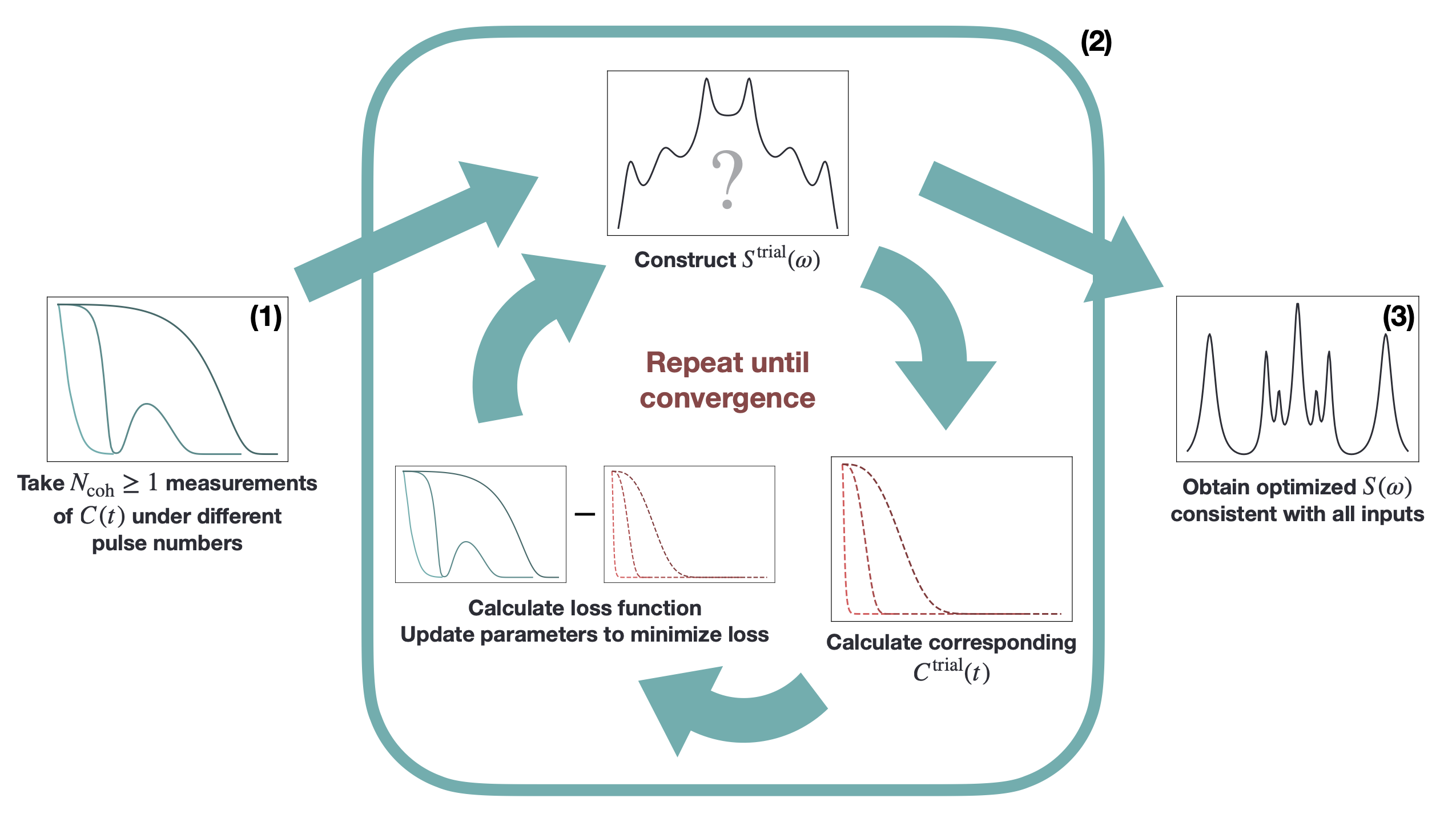
Figure 1: Schematic for the global noise spectroscopy (GNS) protocol. (1) Measure one or more coherence decays under FID, SE, or CPMG dynamical decoupling pulse sequences. (2) Use the measurements as input into our iterative optimization that minimizes the deviation of the measured and trial coherences obtained from a trial spectrum by modifying the coefficients of a Lorentzian basis expansion. (3) Our GNS yields a converged trial spectrum once the iterative loop satisfies an error threshold, $\xi$, for the deviation-based loss function.

Here, we propose and demonstrate such an approach, which we call the global noise spectroscopy (GNS) method. Like DDNS and FTNS, GNS tackles the pure dephasing limit, appropriate in quantum information processing and sensing technology based on nitrogen vacancy (NV) centers [63], trapped ions [55, 64], and neutral atoms [65, 66]. We construct an optimization-based engine that takes as input $N_{\rm coh}\geq 1$ coherence measurements subject to pulse sequences and outputs a predicted noise spectrum simultaneously consistent with all input coherence measurements up to the specified error threshold. We efficiently minimize the loss function that quantifies the agreement of the prediction and the input by leveraging a basis of analytical responses for arbitrary Lorentzian power spectra arising from the application of arbitrary pulse sequences, including but not limited to Ramsey (FID), Hahn echo or spin echo (SE) [1], and arbitrary Carr-Purcell-Meiboom-Gill (CPMG) [2, 3] pulse sequences. We then harness the power of modern statistical noise-robust optimization algorithms [67] to find the optimal set of Lorentzians that reproduce the experimental noise spectrum. We show that our optimization-augmented noise spectroscopy protocol correctly reconstructs multi-Lorentzian, Ohmic, and even $1/f$-type noise spectra [68], and is robust to underconverged experimental measurements and low temporal resolution. Due to its statistical construction, our protocol quantifies the confidence interval of its predictions. We further couple these confidence intervals with measures of the frequency sensitivity of various pulse sequences to guide users on which experimental pulse sequence can selectively improve the confidence interval over a localized frequency range. Finally, we demonstrate our method’s ability to process experimental data from measurements on NV centers. Our GNS correctly identifies the presence of hydrogen nuclei near the NV surface which DDNS had missed, and which required orthogonal measurements to find in the original study [54], attesting to the increased sensitivity that our method offers as a quantum sensing protocol. Figure 1 shows a schematic overview of our GNS method.

II Theory

Under the pure dephasing condition, the timescale associated with population relaxation ($T_{1}$) is much longer than that of phase randomization ($T_{2}^{*}$). In this limit, the qubit Hamiltonian can be written as $\hat{H}=\frac{1}{2}\left[\Omega+\hat{\beta}(t)\right]\hat{\sigma}_{z}$, where $\Omega$ is the natural frequency of the qubit, and $\hat{\beta}(t)$ is the bath noise operator responsible for the fluctuations in qubit energy levels that cause dephasing. When $\hat{\beta}(t)$ is a stationary process obeying Gaussian statistics (i.e., $\langle\beta(t)\rangle=0$, $C(t_{1},t_{2})=\langle\beta(t_{1})\beta(t_{2})\rangle=C(t_{1}-t_{2})$, and all cumulants higher than second order are zero), the coherence function $C(t)=|\langle\rho_{01}(t)\rangle|$ subject to a control pulse sequence can be expressed as

$$C(t)=e^{-\chi(t)}=\mathrm{exp}\left[-\frac{1}{4\pi}\int_{-\infty}^{\infty}d\omega\,S(\omega)F(\omega t)\right].$$ (1)

The noise power spectrum, $S(\omega)$, is the central objective in noise spectroscopy [69, 33, 23, 36]. It is the Fourier transform of the symmetrized equilibrium time autocorrelation function of the Gaussian noise operator, $S(\omega)=\int_{-\infty}^{\infty}dt\,e^{i\omega t}\frac{1}{2}\langle\hat{\beta}(t)\hat{\beta}(0)+\hat{\beta}(0)\hat{\beta}(t)\rangle$. The filter function, $F(\omega t)$, is the Fourier transform of the switching function that encodes the temporal distribution of $\pi$ pulses that are applied to the system [69, 70, 71, 72]. Yet, while filter functions are known analytically, and one may use experimental techniques like NMR or EPR to measure the resulting coherence functions, $C(t)$, extracting the underlying $S(\omega)$ for an experimental system under the application of an arbitrary control pulse sequence remains a fundamental challenge. This is because it is generally impossible to analytically invert Eq. 1 for arbitrary pulse sequences to recover $S(\omega)$.

DDNS circumvents this difficulty by working in the limit of infinitely many applied pulses, $N_{p}\rightarrow\infty$, which allows one to approximate $F(\omega t)$ as a sum of Dirac $\delta$ functions, collapsing the integral and simplifying the reconstruction process. By further approximating $F(\omega t)$ as a single Dirac $\delta$ function [33, 53], one can relate the value of the coherence function under the application of a large $N_{p}$ pulse sequence at a particular time $T^{*}$ to the value of the noise spectrum at a particular value of $\omega^{*}$,

$$S(\omega^{*})\approx-\frac{\pi}{T^{*}}\ln C(T^{*}).$$ (2)

However, this limit requires severe approximations, including the $\delta$ function approximation of the filter function and the need to truncate the infinite sum of $\delta$ functions [73]. Further, the need to apply many pulses renders this procedure experimentally expensive.

To overcome the challenges of DDNS, FTNS offers an exact inversion of Eq. 1 for common FID and SE measurements (0 and 1 DD pulses applied, respectively). FTNS removes practical limitations of DD-based methods, offering access to a greater frequency range and resolution, but at the cost of measurements with high temporal resolution and low statistical noise thresholds ($<1\%$).

Our GNS bridges DDNS’s robustness to experimental imperfections in the measured signal and compatibility with multiple pulse sequences with FTNS’s exact treatment of the response integral and access to the noise spectrum over a broad range of frequencies and with high resolution. We achieve this by reformulating the reconstruction of the noise spectrum as an optimization problem that minimizes the error between the coherences arising from the real noise spectrum, $S(\omega)$, and those arising from a trial noise spectrum, $S^{\rm trial}(\omega)$. In the limit of one coherence measurement subject to a particular pulse sequence, one can formulate the optimization problem as $d|C^{\rm exp}(t)-C^{\rm trial}(t;\bm{\theta})|^{2}/d\bm{\theta}=0$, where $\bm{\theta}$ denotes a set of parameters that can be used to construct a sample noise spectrum, $S^{\rm trial}(\omega,\bm{\theta})$, that determines the shape of the trial coherence curve, $C^{\rm trial}(t;\bm{\theta})$.

How should one pick the parameters $\bm{\theta}$? For example, $\bm{\theta}$ may be the coefficients in a functional expansion of $S^{\rm trial}(\omega)$ over a complete, orthonormal set of polynomials (e.g., Legendre or Chebyshev). While this is a reasonable approach for many applications [74, 75], computing the trial coherence curve from a trial noise spectrum requires one to perform the integral in Eq. 1. Because this integral is generally not analytically solvable for arbitrary pulse sequences, one must resort to quadrature of highly oscillatory functions over an infinite domain, which is slow and renders the optimization process inefficient. We overcome this challenge by employing an overcomplete Lorentzian basis [76, 77, 78, 79] for which the integral in Eq. 1 can be solved analytically (see Appendix A), even with arbitrary pulse sequences (filter functions) [73]. We represent $S^{\rm trial}(\omega)$ as a sum of $N_{\rm basis}$ symmetrized Lorentzians,

$$S^{\rm trial}(\omega)=\sum_{i=1}^{N_{\rm basis}}L_{i}(\omega),$$ (3)

that satisfy the symmetry of $S(\omega)$. Each Lorentzian,

$$L_{i}(\omega)=B_{i}\left(\frac{\omega_{c,i}^{2}}{\omega_{c,i}^{2}+(\omega-d_{i})^{2}}+\frac{\omega_{c,i}^{2}}{\omega_{c,i}^{2}+(\omega+d_{i})^{2}}\right),$$ (4)

is characterized by three parameters, $B_{i}$, $d_{i}$, and $\omega_{c,i}$. Hence, $\bm{\theta}$ consists of $3N_{\rm basis}$ parameters.

Our variational algorithm for a set of $N_{\rm coh}$ coherence measurements, $\{C_{j}(t)\}$ for $j\in[1,N_{\rm coh}]$, arising from the application of different pulse sequences, consists of:

1. Constructing a trial noise spectrum, $S^{\rm trial}(\omega)$, from the sum of $N_{\rm basis}$ Lorentzian functions ($3N_{\rm basis}$ variational parameters), and initializing these parameters stochastically from uniform distributions: $B_{i}\equiv\tilde{B}_{i}/\omega_{0}\in[0,10]$; $\omega_{c,i}\equiv\tilde{\omega}_{c,i}/\omega_{0}\in[0.1,10]$; and $d_{i}\equiv\tilde{d_{i}}/\omega_{0}\in\delta d[i,i+1]$, where $\delta d=d_{\rm max}/N_{\rm basis}$ and $d_{\rm max}/\omega_{0}=20$. We choose $\omega_{0}$ such that the filter functions span a frequency range of $\sim 20\omega_{0}$. Imposing these conditions improves the efficiency and performance of the parameter optimization.

2. Evaluating the trial coherence curves $\{C_{j}^{\rm trial}(t)\}$ based on $S^{\rm trial}(\omega)$ and the filter functions corresponding to the pulse sequences employed in experiment.

3. Calculating the loss function, $\mathcal{L}$, corresponding to the sum of the mean squared errors (MSE) of the true and trial coherence functions integrated over the measurement times and normalized by the total experimental times $T_{j}$. For discrete-time measurements, $\mathcal{L}=N_{t}^{-1}\sum_{j,k}dt\ |C_{j}(t_{k})-C_{j}^{\rm trial}(t_{k})|^{2}$, where $t_{k}$ are the discrete times over which the measurement was performed and $N_{t}$ is the total number of temporal measurements.

4. Employing a gradient-based optimizer and iterating to convergence, defined by an error threshold, $\xi$, subject to the constraint $\bm{\theta}\geq 0$. We use the Adam or AdamW optimizers, which converge efficiently through adaptive learning rates, underlie optimization protocols in machine learning [80, 81], and are accessible via PyTorch [80].

Upon reaching convergence, this protocol yields one set of optimal variational parameters, $\bm{\theta}^{*}$ that define one optimal trial power spectrum, $S(\omega;\bm{\theta}^{*})$ that minimizes the error in the resulting coherence, $C(t;\bm{\theta}^{*})$, with the measured $C(t)$. For general strategies on how to choose appropriate $N_{\rm basis}$ and $\xi$ values and our choices in this work, we refer the reader to Appendix B.

We can now explain our use of the term ‘global’ in our GNS. GNS employs data from multiple pulse sequences with sensitivity to different frequency ranges simultaneously and self-consistently. The above protocol is valid for any number of coherence measurements but can be expected to work best when one chooses $N_{\rm coh}>1$ coherence measurements with complementary sensitivities. In Sec. III.3, we provide a heuristic guide on how to decide which pulse sequences can improve prediction confidence.

While other noise spectroscopy methods aim to exploit multiple coherence measurements simultaneously and self-consistently  [37, 34], our GNS offers greater generality and systematic improvability. For example, Ref. [37] assumes that the noise spectrum arises from an Ornstein-Uhlenbeck process while Ref. [34] requires the user to fit the measured $C(t)$ to a stretched exponential, thereby sacrificing non-Markovian behavior and high-frequency features of the noise spectrum and the possibility of timescale separation that leads to distinct peak structure in the reconstructed noise spectra. In fact, our GNS offers a systematically improvable means to reconstruct the optimal $S^{\rm trial}(\omega)$ that faithfully reproduces the experimentally observed coherence curves, $\{C_{j}(t)\}$, without assuming any noise model or resorting to system-specific preprocessing of data.

III Results

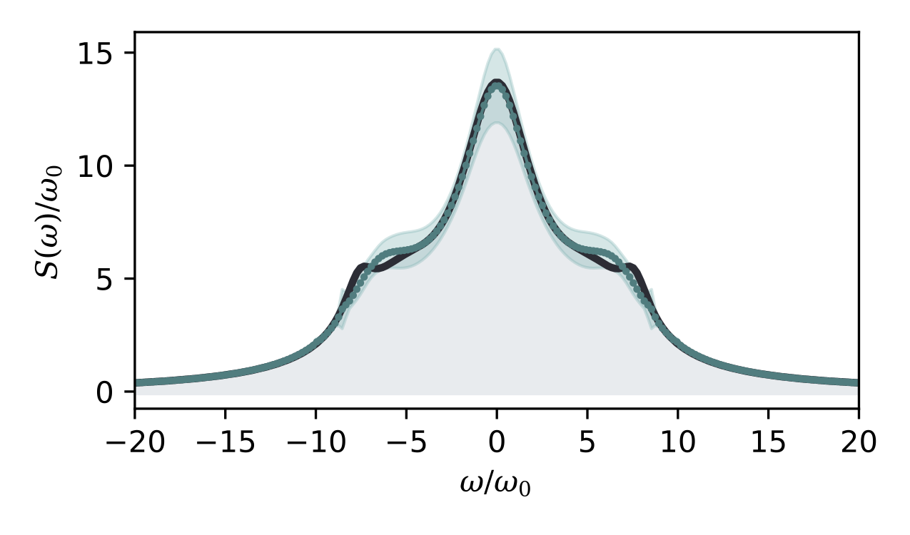
Figure 2: GNS reconstruction of a sample power spectrum from 7 input coherence measurements using 0, 1, 2, 3, 8, 16, and 32-pulse CPMG sequences, a convergence threshold of $\xi=1\times 10^{-5}$, and confidence intervals calculated from $N_{\rm runs}=20$ runs. The solid teal line is the pointwise mean of the reconstructed spectra and the light band is their pointwise standard deviation (confidence intervals). The confidence intervals indicate the frequency regions over which the reconstructed spectrum can be modified, and by how much, for the resulting coherence curves to still agree with the input coherences within the same convergence threshold.

Here, we apply our GNS method to increasingly complex test spectra and highlight its ability to accurately capture features of the true noise spectrum, even under simulated statistical noise in input measurements, and for non-Lorentzian spectra. We then show how our GNS reconstructs the noise spectrum from experiments on shallow NV centers, revealing rich structure corresponding to the presence of identifiable nuclear spins that previous noise spectroscopies had missed. Finally, we introduce a filter function-based analysis that suggests which additional pulse sequence measurements can improve our algorithm’s predictions most efficiently, establishing the GNS’s ability to report on its results’ reliability and delineate a path toward its systematic improvement.

III.1 Application to theoretical data

We first demonstrate the GNS’s ability to reconstruct a structured noise spectrum consisting of a sum of three Lorentzian peaks in Fig. 2. We employ coherence curves under 7 distinct pulse sequences (FID, SE, CPMG2, CPMG3, CPMG8, CPMG16, CPMG32) for this spectrum as input to the optimization scheme, which is given 9 parameters, for $N_{\rm basis}=3$ Lorentzian peaks. We initialize these parameters and optimize them iteratively according to the algorithm outlined in Sec. II and Appendix B.

The stochastic initialization of $\bm{\theta}$ means that each run of the algorithm yields slightly different optimized noise spectra, allowing us to perform statistical analysis to quantify confidence intervals for our noise spectrum predictions. In all our results, we provide the average noise spectrum obtained by performing $N_{\rm runs}$ runs of our algorithm starting from distinct initial conditions subject to the same convergence threshold, $\xi$. We have found that $N_{\rm runs}=20$ is sufficient to converge the mean. The confidence intervals correspond to the pointwise standard deviation of the $N_{\rm runs}$ predictions obtained. We emphasize that $N_{\rm runs}$ is not the same as the number of iterations taken to reach convergence within a single run.

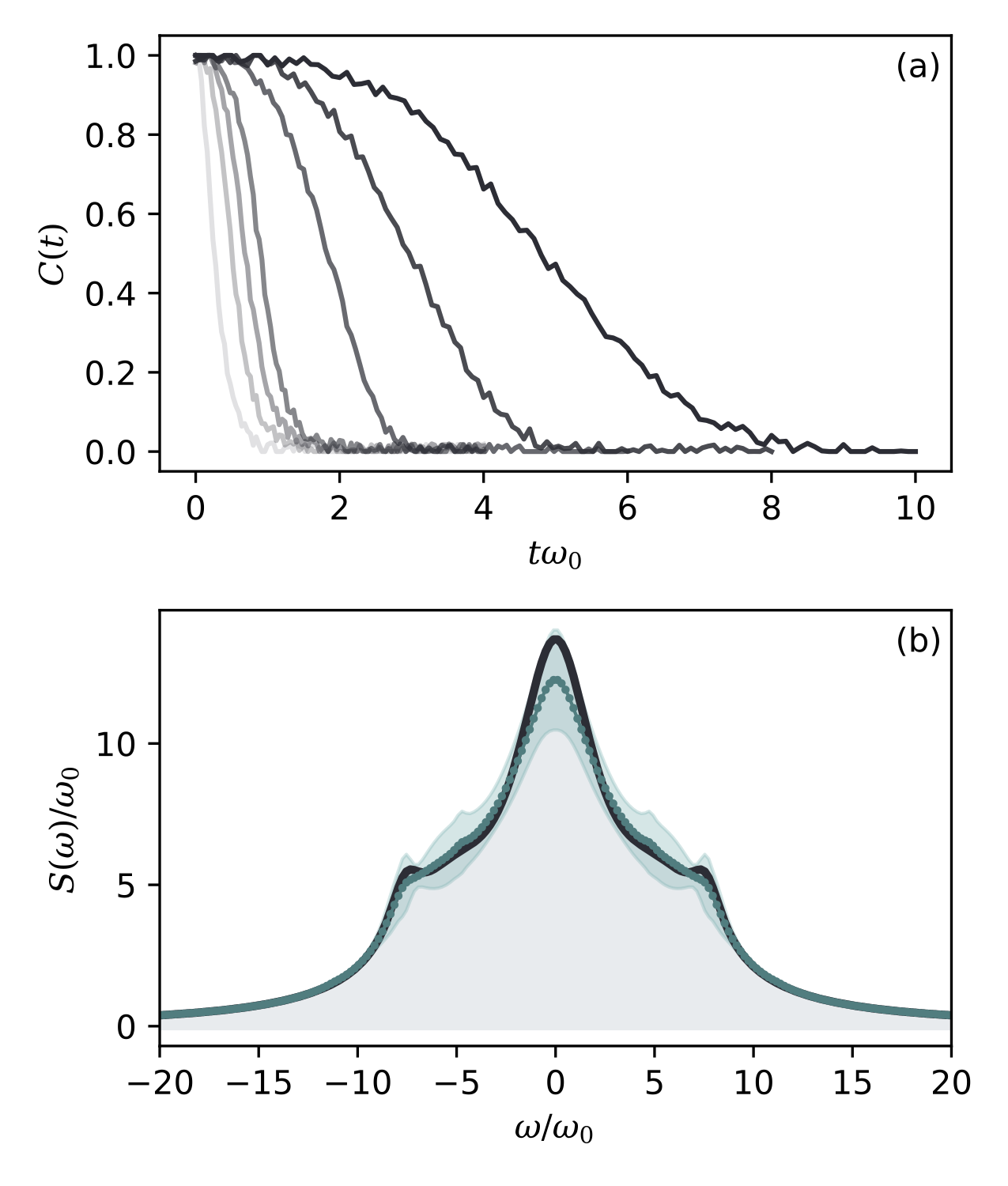
Figure 3: (a) Numerically generated coherence dynamics with simulated measurement uncertainty of 2.0% added on, at different strengths, and (b) the corresponding GNS reconstruction result on these coherence inputs. We used a sample size of $N_{\rm runs}=20$ to quantify the confidence intervals.

Figure 2 shows this average noise spectrum and its standard deviation-based confidence intervals (in translucent teal) subject to $N_{\rm runs}=20$ and $\xi=1\times 10^{-5}$. The confidence intervals correctly reflect the uncertainty in the shoulder feature at $\omega\sim 5$ where the mean predictions deviate slightly from the true spectrum and the fact that the central peak height can vary without significantly affecting overall agreement with input coherence curves. The fact that GNS does not perfectly reconstruct the true spectrum, even for theoretically pristine data, arises from the fact that a set of similar noise spectra can reproduce the same coherence curves within a small error threshold. Nonetheless, this scheme accurately captures the positions, widths, and heights of the constituent Lorentzians. Because our algorithm is trivially parallelizable and highly efficient, with a single iterative run taking $\lesssim 5$ minutes on a commonly accessible laptop, we recommend users performing the statistical analysis obtained from repeated trials as it offers the benefit of quantifying confidence intervals.

We now demonstrate our method’s robustness to experimental uncertainties marring the smoothness of the input coherence data. Figure 3 shows a prediction obtained from coherence inputs with simulated experimental errors obtained by adding a random number to every coherence data point drawn from a uniform distribution spanning $[-\epsilon,\epsilon)$, where $\epsilon=0.02$ quantifies the effective error level. This quantity mimics the effects of all uncorrelated errors in an experimental measurement, including background and shot noises [82]. We evaluate the statistics after $N_{\rm runs}=20$ predictions. We allow the algorithm to employ up to $N_{\rm basis}=10$ Lorentzian basis functions to obtain sufficient functional flexibility and shorten convergence time. Furthermore, because the added error in the target coherences places an upper limit to the achievable loss, we adopt $\xi=1.17\times 10^{-4}$ as the loss threshold.

Remarkably, the average prediction semiquantitatively agrees with the noise-free case in Fig. 2, retaining the salient features of the true spectrum. The true spectrum also largely lies within the confidence intervals at all levels of measurement error. It bears emphasizing that we obtain these results without employing any denoising protocols on the noisy coherence curves. This level of performance in the presence of statistical noise shows that our GNS offers a simple yet powerful means to extract noise spectra from realistic coherence curves, even when highly averaged data is not immediately available.

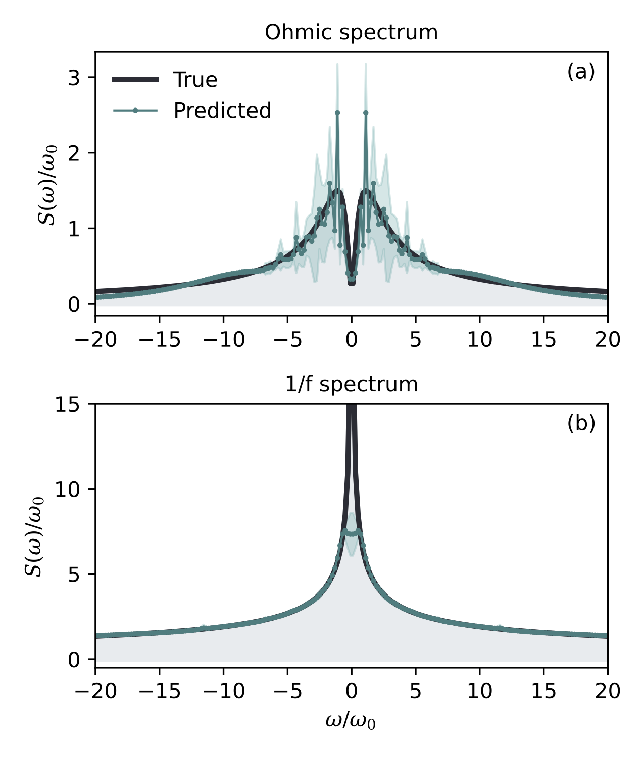
Figure 4: Non-Lorentzian noise spectrum reconstruction of an (a) Ohmic spectrum, and a (b) $1/f$ spectrum. For both spectra, we used $\xi=3\times 10^{-5}$, $N_{\rm basis}=20$, and $N_{\rm runs}=20$.

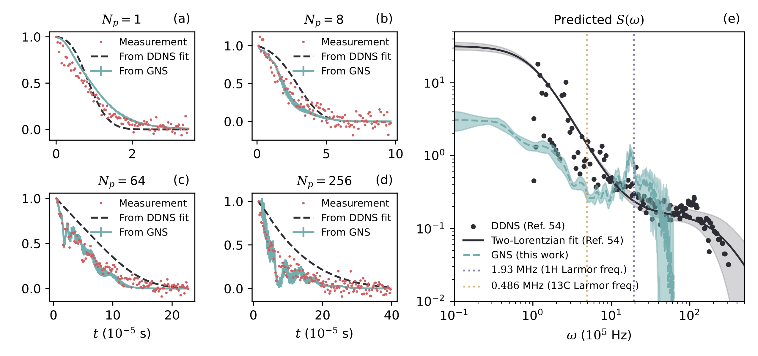
Figure 5: (a-d) Comparison of experimentally measured coherence curves with those predicted using power spectra reconstructed using DDNS and GNS for experiments with 1, 8, 64, and 256 CPMG pulses. (e) Comparison of noise spectra reconstructed using DDNS taken from Ref. [54] (dark blue) and GNS (teal). For the GNS noise spectrum reconstruction, we show confidence intervals as a translucent teal band. Dotted vertical lines indicate the Larmor frequencies of hydrogen (purple) and carbon-13 (yellow) at an applied magnetic field of 454 G. The presence of a peak at the hydrogen Larmor frequency is expected due to the presence of protons from the immersion oil at the surface of the sample, in proximity to the NV center, and is also reported in the original study [54]. The lack of a feature appearing at the carbon-13 Larmor frequency is consistent with and likely due to the fact that the isotopically purified sample used contains $<0.001$% carbon-13 impurities.

While we have demonstrated our protocol’s ability to fit sums of Lorentzian functions to sums of Lorentzian functions, a truly general noise spectroscopy method should be able to predict arbitrary functional forms of the spectrum. Here, we illustrate our GNS’s ability to predict non-Lorentzian spectra. We use as test cases two challenging functional forms: an Ohmic spectrum with an asymptotic inverse linear behavior that decays more slowly than Lorentzians characterized by an asymmetric peak with a long tail at high frequencies, and a divergent $1/f$ spectrum. The Ohmic spectrum takes the form

$$S_{\mathrm{Ohmic}}(\omega)=\eta\frac{|\omega|}{\omega^{2}+\gamma^{2}}$$ (5)

with $\gamma=1.1\omega_{0}$ setting the timescale of decay and $\eta=3.3\omega_{0}$ setting the qubit-environmental coupling energy. The $1/f$ spectrum is given by

$$S_{1/f}(\omega)=\frac{\zeta}{|\omega|}$$ (6)

with $\zeta=6\omega_{0}$ quantifying the qubit-environmental coupling. In the Ohmic case, we employed coherences under 7 CPMG pulse sequences with 0, 1, 2, 3, 4, 5, and 6 pulses to generate the noise spectrum prediction. For the $1/f$ spectrum, we used coherences under 7 CPMG pulse sequences with 1, 2, 3, 4, 8, 16, and 32 pulses. We omit the 0-pulse measurement for the $1/f$ spectrum since the functional divergence of $S_{1/f}(\omega)$ at $\omega=0$ causes the integral in Eq. 1 to diverge for the 0-pulse filter function, which has a nonzero contribution at $\omega=0$. This suggests that a true $1/f$-type spectrum over all frequencies is unphysical. Nevertheless, $1/f$-type power spectra are often invoked to describe the frequency-dependent scaling over finite regions in frequency space, which our GNS accurately captures [68].

Figure 4 shows our GNS reconstructions of the Ohmic and $1/f$ type spectra as described by Eqs. 5 and 6. For each prediction, we allow the algorithm to use $N_{\rm basis}=20$ Lorentzians (60 parameters total), with $\xi=3\times 10^{-5}$ and statistics taken over $N_{\rm runs}=20$ trials. The results show an impressive agreement within confidence intervals, including the slowly decaying high-frequency tails and suppressed contribution near $\omega\rightarrow 0$ in the Ohmic spectrum, and the distinct $1/\omega$-type approach towards zero frequency in the $1/f$ spectrum, confirming the broad applicability of our GNS.

III.2 GNS disentangles complex signals in experimental data

We now demonstrate the ability of GNS to extract frequency-resolved features in the noise spectrum from experimental data. We take pulsed coherence measurements on shallow NV centers used to generate the DDNS-generated noise spectrum given in Fig. 2(e) of Ref. [54] and extract the corresponding noise spectrum using our GNS protocol. We employ all 10 available coherence measurements as input, with 1, 2, 4, 8, 16, 32, 64, 96, 128, and 256 CPMG pulses. For these data, we choose $\omega_{0}=10^{5}/(2\pi)$ Hz. To assess the accuracy of GNS relative to DDNS, we quantify which protocol yields a power spectrum that more faithfully reproduces the experimentally measured coherence curves and resolves features corresponding to nuclear spin species expected to lie near the diamond surface.

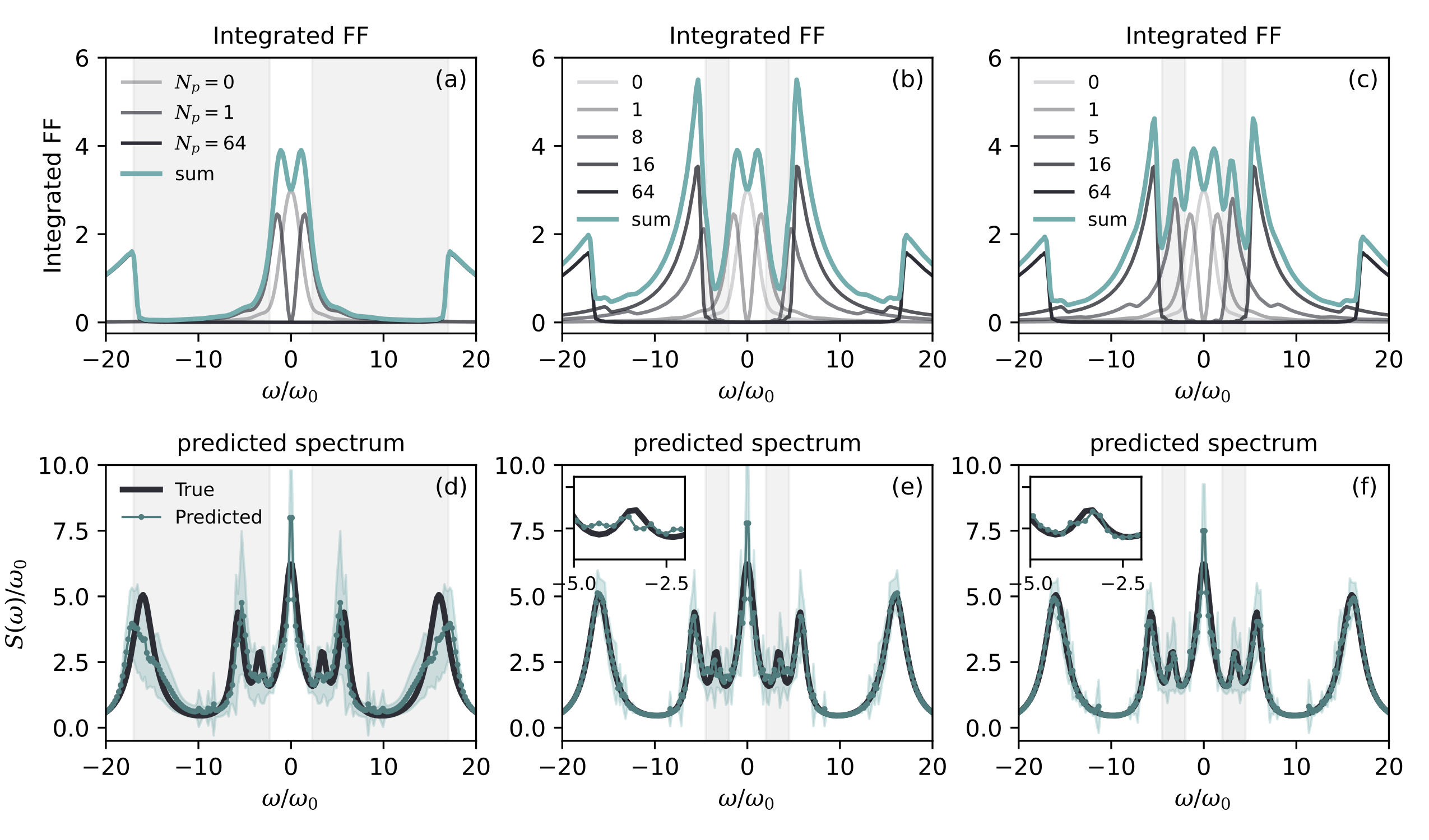
Figure 6: (a-c) Filter functions of pulse sequences used in the measurement set integrated over total measurement time as a function of frequency. (d-f) Noise spectra reconstructed using the corresponding sets of measurements indicated in the above panels. For the spectrum reconstructions, we used $N_{\rm basis}=20$, $N_{\rm runs}=20$, and $\xi=1\times 10^{-5}$. Insets of (e) and (f) show a close-up view of the mean prediction and true spectrum values at the peak located at $\omega\approx-3.4\omega_{0}$, where the addition of the CPMG5 sequence in (f) improves the ability of the method to predict the presence of this peak compared to (e).

Figure 5(e) shows the result of performing our GNS method on all 10 available sequences, with selected coherence measurements and coherence curves generated from reconstructed spectra given in panels (a-d). For this noise spectrum reconstruction, we adopt $N_{\rm runs}=30$, $\xi=1\times 10^{-2}$, and $N_{\rm basis}=40$ Lorentzian basis functions. Compared to the spectrum obtained using DDNS in Ref. [54], GNS predicts the low-frequency component to be about an order of magnitude smaller than projected by the double-Lorentzian fit proposed in the original work, implying that inhomogeneous disorder plays a significantly reduced role in decoherence than previously expected. As the figure shows, DDNS reconstructions have a hard cutoff around the $\omega\sim 0.1$ MHz, below which no further information about the spectrum is accessible. Approaching this cutoff from the right, one can also notice that the spread of the DDNS predictions of the spectrum amplitude becomes larger, so that by the lowest frequency range, the reconstructed points vary by close to two orders of magnitude. These factors make it difficult for the DDNS reconstructions alone to inform the behavior of the spectrum as $\omega\rightarrow 0$, which may explain the discrepancy observed. In contrast, the confidence intervals of our GNS predictions vary only by a factor of 1.5 to 2 for $\omega\leq 20$ MHz. Crucially, Fig. 5 (a-d) reveal that the coherence curves corresponding to the GNS-reconstructed spectrum display markedly better agreement with the measured coherences across all shown CPMG pulse numbers, compared to the coherence curves arising from the double Lorentzian fit obtained from the traditional DDNS-type analysis. The GNS-enabled insight that the DDNS reconstruction overestimates the importance of the low-frequency part of the noise spectrum aligns with the observation that the DDNS spectrum best reproduces the SE decay in Fig. 5 (a) but progressively worsens in capturing the coherences for all higher pulse sequences in Fig. 5 (b-d). Hence, one may confidently say that our GNS noise spectrum reconstruction offers narrower error bars and greater consistency with the experimentally measured coherence curves.

Having established the reliability of our GNS noise spectrum reconstructions, the most striking feature of our GNS prediction compared to that of DDNS is the wealth of structure in the spectrum. In particular, the GNS spectrum contains a prominent peak at $\approx 1.93$ MHz, which corresponds to the Larmor frequency of hydrogen at the magnetic field strength under which the measurements were performed (454G)—a feature which was also reported in [54], but which was only visible under separate measurements using an XY8 pulse sequence. This signal is associated with the proximity of the NV center to the surface on which there is an abundance of protons from hydrogen atoms in the immersion oil (for a discussion on the origin of the minor shift in position from the expected hydrogen Larmor frequency value, we refer the reader to Appendix C). Further, the lack of a feature of similar prominence at the corresponding carbon-13 Larmor frequency ($\approx 0.5$ MHz) is consistent with the experiment’s use of an isotopically purified sample containing $<0.001\%$ carbon-13 impurities. Thus, our GNS’s ability to resolve this feature from the CPMG measurements alone—a feat that the previous state-of-the-art method, DDNS, was unable to achieve—attests to the method’s power in extracting more physical insight from the same amount of data, i.e. performing noise spectroscopy more accurately and efficiently.

III.3 Choosing additional measurements

Equation 1 makes clear that when the filter function associated with a particular pulse sequence becomes small, spectral reconstruction becomes more uncertain. Hence, no single pulse sequence fully reveals the spectrum across all frequencies. One may, therefore, suppose that there exist complementary sequences that, when taken together, give access to the noise spectrum across a wide range of frequencies. We offer a heuristic for determining this complementarity via “integrated” filter functions.

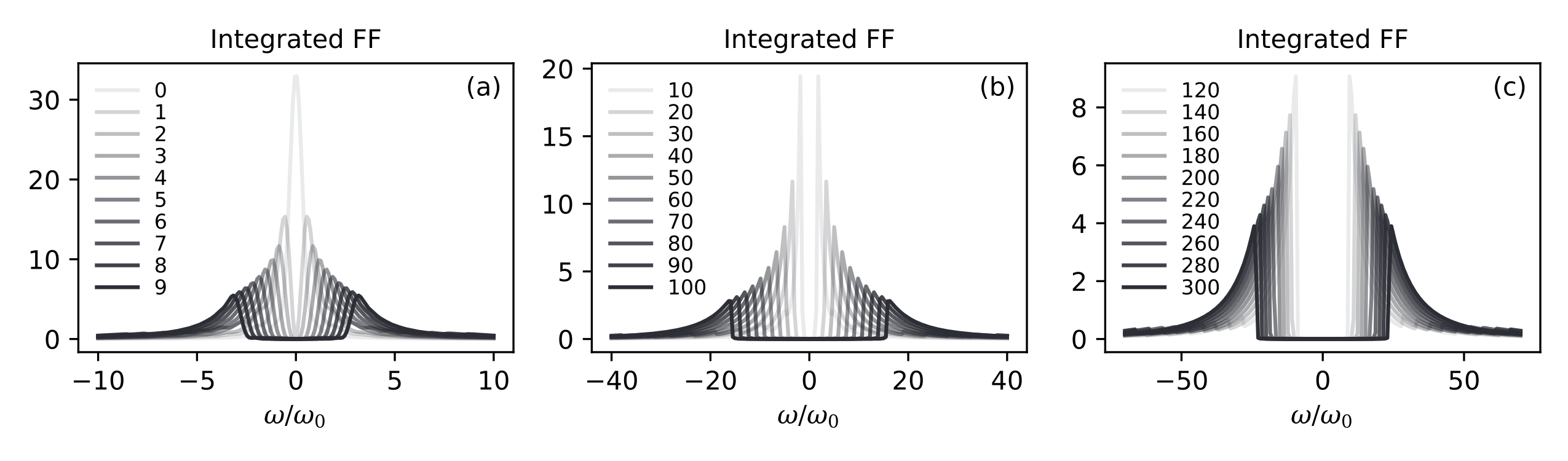
Figure 7: Integrated filter functions of selected CPMG-$N$ pulse sequences. The legend specifies the number of pulses in each CPMG sequence. For all functions shown, we used $t_{i}=0$. Because assigning a $t_{f}$ in the absence of a particular form of the noise spectrum is difficult, we adopt $t_{f}=10\omega_{0}^{-1}$ for Fig. 7(a), $t_{f}=20\omega_{0}^{-1}$ for (b), and $t_{f}=40\omega_{0}^{-1}$ for (c).

To test our proposed heuristic, we quantify our GNS’s ability to reconstruct a structured test spectrum subject to pulse sequences that exhibit “blind spots” over relevant frequency ranges compared to pulse sequences that cover these blind spots. The results are shown in Fig. 6. The Integrated FF offers a frequency-resolved measure of a pulse sequence’s ability to reveal the noise spectrum,

$$I_{x}(\omega)=\frac{1}{t_{f}-t_{i}}\int_{t_{i}}^{t_{f}}F_{x}(\omega t)\,dt$$ (7)

where $F_{x}(\omega t)$ is the filter function for the $x$-sequence, where $x$ can denote FID, SE, CPMG sequences with $N_{p}$ pulses, or others. $t_{i}$ and $t_{f}$ are the initial and final time from and up to which the $N_{p}$-pulse coherence is measured, respectively. We introduce the sum of integrated filter functions to quantify the collective sensitivity of a set of pulse sequences. Qualitatively, the frequency regions of low sensitivity, i.e., low amplitude in the summed integrated filter functions, correspond to regions in the reconstructed spectra where the predictions vary significantly (shaded in gray), as indicated by the broad confidence intervals, in Fig. 6 (a) and (d). Comparing Fig. 6 (a) and (b) shows that adding measurements of 8- and 64-pulse CPMG sequences largely remedies this valley of low sensitivity. As hypothesized, Fig. 6 (e) demonstrates that the variations in the predictions narrow significantly in the corresponding frequency range as compared to Fig. 6 (d). Nevertheless, the frequency region $\omega\in[2,5]\omega_{0}$ remains difficult to resolve under this combination of pulse sequences, as indicated in the inset in (e) which zooms into the true spectrum and mean prediction in this frequency region. Noting that a 5-pulse CPMG sequence provides the necessary weight in this frequency range (Fig. 6 (c)), replacing the 8-pulse CPMG sequence with the 5-pulse CPMG sequence allows the previously hidden small peaked feature at $\omega\approx 3.4\omega_{0}$ to emerge in the averaged spectrum prediction, as shown in the inset of Fig. 6 (f). Thus, these results indicate that the integrated filter function quantifies the sensitivity of various pulse sequences to noise spectra over specified regions of frequency space.

This analysis supports our proposed heuristic for selecting the pulse sequences that optimally improve spectrum reconstructions. Specifically, one can generate a set of integrated filter functions for the available measurements and obtain their sum. This quantifies the frequency ranges over which the spectrum prediction is likely to be less reliable due to diminished sensitivity in the measurements. One can then augment the existing measurements with complementary pulse sequences. To selectively enhance sensitivity over a particular frequency window, one should select pulse sequences whose integrated filter functions add the most weight to the region of interest, usually the region displaying the lowest weight in the summed integrated filter functions for the existing measurements. Figure 7 provides a visual guide of the integrated filter functions for selected CPMG-$N$ pulse sequences. This protocol can be expected to facilitate more reliable noise reconstructions with suppressed variance and narrow confidence intervals.

A consequence of this analysis is that predictions arising from any noise spectroscopy protocol yield coherence dynamics that are insensitive to large spectral fluctuations regions with limited filter function sensitivity. Indeed, Eq. 1 dictates that the coherence arising from a sum of spectra is equal to the product of the coherences arising from these spectra individually,

$$C(t) =\mathrm{exp}\left[-\frac{1}{4\pi}\int_{-\infty}^{\infty}d\omega\,\sum_{i}S_{i}(\omega)F(\omega t)\right]=\prod_{i}C_{i}(t).$$ (8)

That is, for a given pulse sequence, components of the spectrum that cause a fast decay of the coherence (generally low-frequency structures) suppress long-lived features that arise from other components of the noise spectrum (generally high-frequency features), leading to the effective “blindness” of the sequence to such features. Thus, it is critical to ensure that predictions do not exhibit unphysical features in regions of limited frequency sensitivity. We enforce this constraint via mild regularization to penalize large fluctuations in regions in which any change in the prediction minimally affects the loss (see also Appendix C for details).

III.4 Versatility, interpretability, and efficiency

Our GNS design and implementation choices arise from our commitment to leveraging experimentally accessible measurements while reducing their cost, satisfying stringent reproducibility criteria, enhancing signal-to-noise ratio in extracting noise power spectra, and offering a portable and efficient code base that practitioners can easily incorporate into their workflow, enabling its use in on-the-fly interrogation of noise in quantum technology.

Like DDNS [32] and FTNS [62], our GNS applies to the pure dephasing limit where decoherence is induced by Gaussian noise. While DDNS is limited to pulsed coherence measurements satisfying the spectroscopic limit [73] where the pulse number must be sufficiently high for the $\delta$ function approximation to hold and FTNS is restricted to the FID and SE coherence decays, our GNS does not have similar restrictions. Indeed, our GNS accepts measurements under any number of CPMG (and even non-CPMG) pulse sequences. This opens a much wider set of measurements under “intermediate number” DD pulses that can reliably be used to inform the predicted noise spectrum, thus ensuring that GNS can effectively leverage experimentally accessible measurements. We compare the performances of FTNS and GNS in Appendix D.

GNS also offers attractive features that facilitate uncertainty quantification, reproducibility, as well as systematic improvability in noise spectrum reconstructions. Because our proposed GNS algorithm performs a variational optimization on stochastically initialized basis parameters, the results of independent runs converge to power spectra that differ from each other. The extent to which these predictions vary offer a means to quantify the confidence intervals of our predictions, such that narrower confidence intervals indicate the robustness and reproducibility of the power spectrum reconstruction. These confidence intervals primarily depend on three factors: (i) the signal’s temporal resolution, (ii) the error bars of the coherence measurements, and (iii) the spectral region of sensitivity of the applied pulse sequences. The temporal resolution, for example, sets an upper limit on the maximum frequency that our reconstruction can resolve. In the limit of low to no experimental noise, our GNS can accurately reconstruct the noise spectrum in the Fourier-transform allowed region. Even in the Fourier transform-forbidden regions, our GNS reconstructions remain largely accurate (see our model reconstructions in Fig. 3 and Fig. 9(d) in Appendix D) because of its use of a physically motivated Lorentzian basis. However, in the limit of large experimental measurement errors (second factor) which mask as high-frequency oscillations, our GNS’s ability to optimally reconstruct power spectra that faithfully reproduce coherence measurements leads to unphysical high-frequency features. To tame these features, we suggest three options: additional experimental measurements to reduce experimental error, batch subsampling to check for consistency, and mild regularization (see our experimental reconstructions in Appendix C). To address the third factor of spectral sensitivity, we developed and showed the viability of our time-integrated filter function heuristic to determine which pulse sequence one should use to improve confidence intervals (see Fig. 6).

The portability and efficiency of our GNS are ensured by our choice of variational basis (Lorentzians) and adoption of state-of-the-art optimization algorithms that have now become the norm in machine learning approaches. We opt for a Lorentzian basis because of the need to efficiently evaluate the loss function in our variational procedure, which requires one to repeatedly calculate the coherence decays that arise from the application of a set of pulse sequences to a trial power spectrum (see Eq. 1). The availability of analytical expressions for the coherence response due to an arbitrary Lorentzian power spectrum subjected to any applied pulse sequence [73] obviates the need for numerical quadrature, rendering the evaluation of our loss function highly efficient. We note, however, that one may also consider different basis functions, such as Gaussians [73] or purely positive polynomials [83], (albeit at the cost of lower efficiency for functions which do not have analytical expressions available).

We implement our variational algorithm in Sec. II using PyTorch [80], which provides built-in functions for efficient optimization and offers a convenient framework to set up our iterative procedure. The computational cost required for this method is small, generally taking $3-5$ minutes on a commercial laptop with 16GB memory and an Apple M1 chip for a single run. Because the algorithm is trivially parallelizable, one can perform independent runs to estimate statistics and quantify confidence intervals simultaneously across cores. As an illustrative example, we note that the individual optimization that took the longest time ($\sim 30$ minutes) was for Fig. 4(a).

IV Conclusions

We have introduced a new theoretical tool, our GNS, that post-processes coherence measurements subject to arbitrary pulse sequences—commonly performed in quantum optics, chemistry, and atomic and molecular physics experiments around the world—to characterize the decoherence mechanisms of quantum systems. Our GNS establishes a variational principle that enables us to construct an efficient, effective, and simple algorithm that predicts a power spectrum that simultaneously and optimally reproduces experimental measurements. We have demonstrated its accuracy and efficiency in reconstructing power spectra that are traditionally considered challenging for existing noise spectroscopy protocols, including $1/f$ (divergent as $\omega\rightarrow 0$) and Ohmic (slowly decaying) power spectra. We have further shown that our GNS’s noise spectrum reconstructions are robust to the presence of statistical experimental error arising from limited measurement averaging and limited temporal resolution, opening the door to its use on fast and accessible measurements. This is particularly important when one considers that, while measurement errors can be minimized even with limited repetitions in ensembles of quantum systems (e.g., molecular magnets in solution or a glass matrix, or collections of NV centers in a macroscopic diamond sample), obtaining sufficient statistics in the single quantum sensor limit becomes prohibitively experimentally expensive.

We have formulated our GNS to specifically address widely targeted goals of quantum sensing: the pure dephasing limit, which applies to a wide variety of quantum platforms, and the Gaussian limit, which remains the primary framework for doing noise spectroscopy [32, 40, 62, 34, 37, 53, 54, 33, 84]. Compared to previous state-of-the-art methods like FTNS and DDNS, our GNS offers greater robustness to experimental errors and low temporal resolution in the coherence measurements, access to a greatly expanded range in frequency, and even higher frequency resolution. What is more, GNS allows for rigorous uncertainty quantification via frequency-resolved confidence intervals, integrated filter-function based sensitivity analysis, and strategies such as batch subsampling of input measurements and sensitivity tests to regularization strength in the optimization algorithm allowing. These strategies empower users to verify consistent features in the predictions.

Our GNS is also simple and efficient. Our PyTorch implementation exploits modern state-of-the-art optimization algorithms and a physical expansion basis that enables fast evaluation of the loss function and, hence, optimization. The algorithm is also trivially parallelizable. Taken together, this means that our GNS is sufficiently efficient to enable on-the-fly characterization of the noise spectrum and iterative improvement of experiments as they happen, especially when coupled with our integrated filter function heuristic for choosing refining experiments.

The success of our GNS in revealing the unexpectedly small influence of low-frequency noise and correctly resolving the ¹H signal—which DDNS misses—and the absence of the ¹³C peak in the power spectrum in experiments on a NV sensor in isotopically purified diamond immersed in oil [54] suggests that a wealth of physical insight stands to be gained even from future and currently available measurements that are yet to be exploited. The accuracy, simplicity, and generality of our GNS set the stage to achieve error-resilient and scalable precision quantum sensing across many quantum platforms. As the power spectrum is the central objective of quantum sensing protocols that aim to obtain a frequency-resolved characterization of the sensor-environmental coupling, we anticipate that GNS will become a central tool in enabling precision quantum sensing.

Appendix A Attenuation functions for Lorentzian spectra subject to CPMG pulse sequences

Here, we provide expressions for the attenuation function for a symmetrized Lorentzian function (as given in Eq. 4), restricted to CPMG pulse sequences ($N_{p}\geq 1$), as a function of $N_{p}$ and the parameters of the Lorentzian. $\chi_{\rm CPMG}^{\rm even}$ refers to the expression for the case where $N_{p}$ is even and $\chi_{\rm CPMG}^{\rm odd}$ where $N_{p}$ is odd.

$$\chi_{\mathrm{CPMG}}^{\rm even}(t,N_{p}) = \frac{Bt\omega_{c}^{2}}{\omega_{c}^{2}+d^{2}}+\sum_{z\in\{z_{-},z_{+}\}}\frac{iB\omega_{c}\left(N_{p}\tan\left(\frac{tz}{2N_{p}}\right)+4e^{-\frac{1}{2}itz}\sin\left(\frac{1}{2}tz\right)\sin^{4}\left(\frac{tz}{4N_{p}}\right)\sec^{2}\left(\frac{tz}{2N_{p}}\right)\right)}{z^{2}},$$ (9)

and

$$\chi^{\rm odd}_{\mathrm{CPMG}}(t,N_{p}) = \frac{Bt\omega_{c}^{2}}{\omega_{c}^{2}+d^{2}}+\sum_{z\in\{z_{-},z_{+}\}}\frac{B\omega_{c}\left(\left(1-e^{\frac{itz}{2N_{p}}}\right)^{4}\left(1+e^{-itz}\right)-2N_{p}\left(1-e^{\frac{2itz}{N_{p}}}\right)\right)}{2\left(1+e^{\frac{itz}{N_{p}}}\right)^{2}z^{2}},$$ (10)

where $z_{+}\equiv d+i\omega_{c}$ and $z_{-}\equiv d-i\omega_{c}$.

Appendix B Optimizer settings and convergence parameters

Here, we offer details on the optimizers and hyperparameters we used to generate all figures in this manuscript. We also outline general strategies to satisfy reproducibility criteria and select appropriate convergence thresholds. For all figures, we employed our PyTorch implementation of an iterative optimization scheme using the Adam or AdamW optimization algorithm. The iterative minimization of the loss function repeats until the MSE loss value falls below the $\xi=1\times 10^{-5}$ threshold. If the loss fails to converge to the required threshold within 10000 iterations, we terminate the procedure and restart it with new initial parameters.

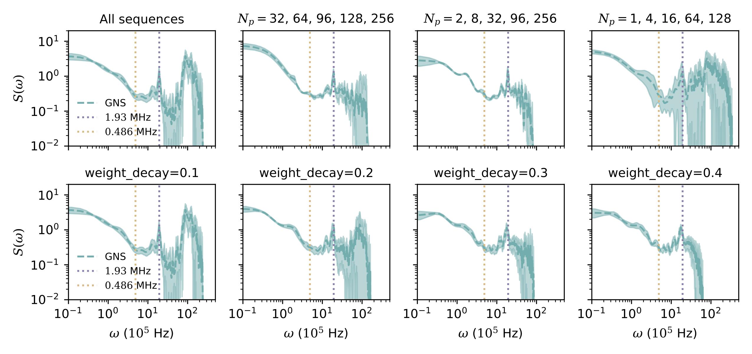
Figure 8: GNS predictions of the noise spectrum of a NV quantum sensor in diamond from experimental measurements reported in Ref. [54] and used in Sec. III.2 in the main text, using different subsamples of the available measurements as input (top row), and varying the regularization strength in the optimizer (bottom row). Across both tests, the peak at the hydrogen Larmor frequency (indicated by the purple dashed vertical line) appears consistently, suggesting its veracity. Also across both tests, an additional structure at higher frequency regions ($>3\times 10^{5}$ Hz) and at the carbon-13 Larmor frequency (indicated by the yellow dashed line) fail to manifest consistently, indicating their possible spurious nature.

We opted for the Adam optimizer to generate Figs. 2, 3, and 6, with the learning rate hyperparameter lr=0.01. For Fig. 4, we used AdamW, which decouples the weight decay in the regularization from the optimization steps, offering a more efficient implementation of regularization [85]. We use the hyperparameters lr=0.01, eps=1e-6, weight_decay=0.01, and betas=(0.9, 0.9). For Fig. 5, we use the AdamW optimizer with hyperparameters lr=0.02 and weight_decay=0.4. For Figs. 9 and 10, we used the AdamW optimizer with hyperparameters lr=0.01 and weight_decay=0.1.

To ensure the reproducibility of the reconstructed noise spectra, the optimization process should converge with increasing flexibility and the number of variational parameters (i.e., the size of the basis used to reconstruct the spectrum, $N_{\rm basis}$). Consequently, all our predictions are in the limit where the results converge with respect to $N_{\rm basis}$ subject to a chosen iterative error threshold, $\xi$. To achieve this, it is beneficial to perform reconstructions with increasing $N_{\rm basis}$, check that each choice of $N_{\rm basis}$ can satisfy the error threshold, $\xi$, and confirm that the reconstructed spectra from these runs fall within the target confidence intervals.

To choose the convergence threshold, $\xi$, which allows one to enhance the signal-to-noise ratio, one should perform simple preliminary tests that account for the level of experimental uncertainty in the available measurements. Specifically, one should choose an initially conservative estimate (e.g., $\xi^{\rm trial}=10^{-5}$) based on the level of uncertainty present in the input signals, and run the optimization a few times. If the loss function plateaus at a consistent but higher value, $\xi^{\rm new}>\xi^{\rm trial}$, throughout these tests, one should adopt $\xi^{\rm new}$ as the new convergence threshold for efficient performance. Conversely, if the optimizations easily reach $\xi^{\rm trial}$, one should lower this threshold to quantify the level of agreement the optimizer can effectively achieve. Generating confidence intervals based on these runs indicates whether the applied convergence threshold is sufficiently small to give reliable predictions.

Appendix C Sensitivity analysis on GNS predictions of experimental data

Here, we outline strategies for verifying the predicted features obtained using the GNS method when one is limited to an available set of measurements. An accessible approach would be to study the predictions made on different subsets of the available measurements to confirm which features are predicted robustly across different subsamplings. Features that do not consistently appear across different subsamplings indicate that these may not be reliable. Furthermore, when accessible measurements display high measurement uncertainties, we recommend adjusting the level of regularization implemented in the optimizer to identify and suppress features that may be a consequence of the measurement uncertainty rather than the true signal.

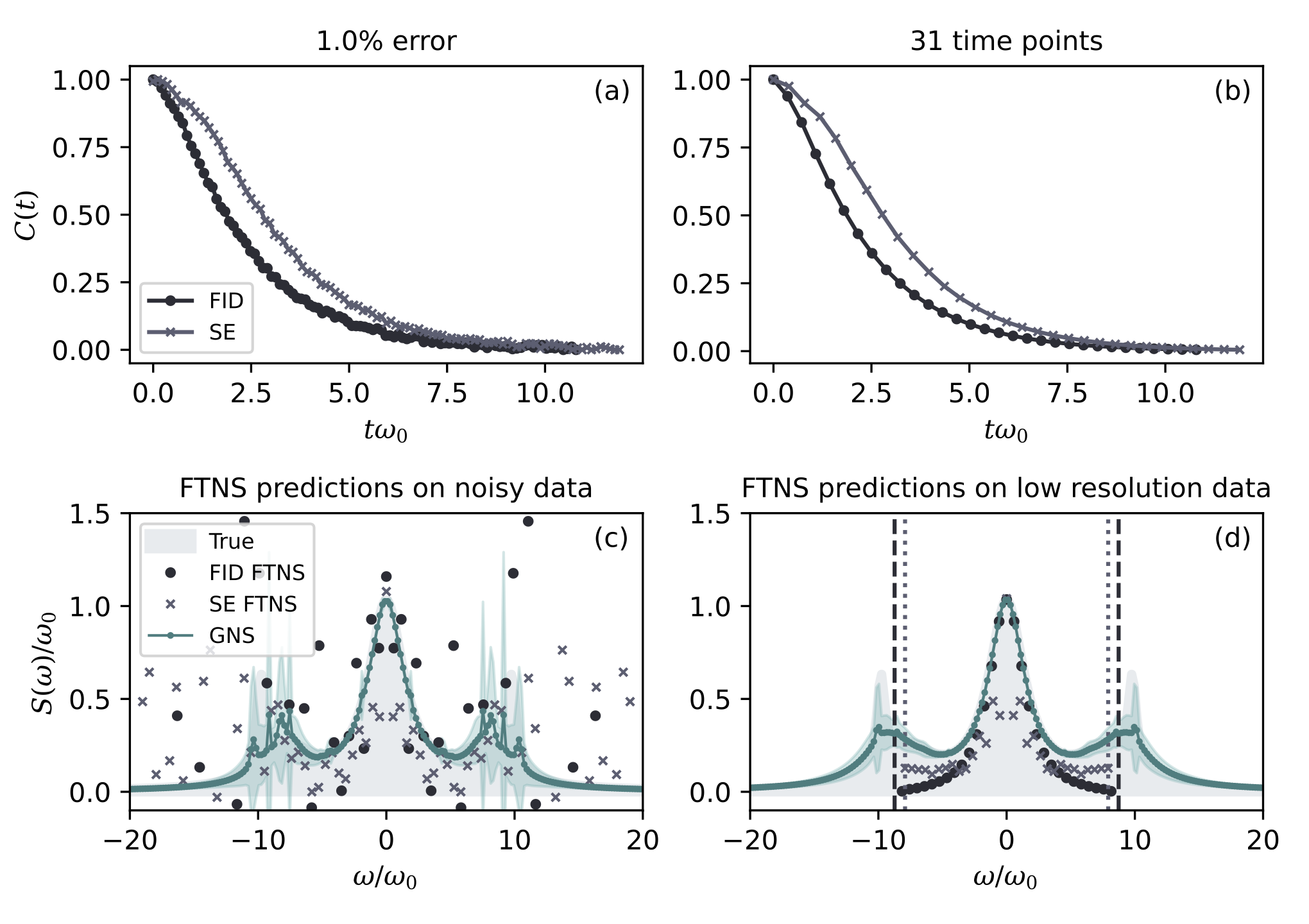
Figure 9: (a, c) Comparison of FID FTNS, SE FTNS, and GNS with FID and SE measurements with 1.0% added simulated measurement noise. FTNS methods are sensitive to measurement uncertainties, whereas GNS shows robustness against these. We employ a loss threshold of $\xi=3.5\times 10^{-5}$, $N_{\rm basis}=3$, and $N_{\rm runs}=20$. (b, d) Comparison of FID FTNS, SE FTNS, and GNS power spectrum reconstructions for coherence input with 31 total measurement points. For FTNS, the temporal resolution of measurements directly translates into limits of frequencies up to which the spectrum reconstruction can be performed reliably (dashed and dotted vertical black lines in (d)) but GNS can overcome such limitations even for low measurement resolution. For these data, we use a loss threshold of $\xi=1\times 10^{-6}$, $N_{\rm basis}=3$, and $N_{\rm runs}=20$.

In Figure 8, we show the results of applying both tests to the experimental data used in Sec. III.2 of the main text. The first row of the figure shows spectrum predictions obtained from the application of GNS with the AdamW optimizer with hyperparameters lr=0.02 and weight_decay=0.1 to different subsets of the 10 available CPMG measurements. Interestingly, while all subsets consistently predict the presence of the prominent hydrogen Larmor frequency peak (purple vertical dashed line), the broad higher-frequency feature only appears in two of the four cases considered. This indicates that the structure predicted in the highest frequency region may not be as reliable. To further test this, in the second row of the same figure, we show the results of GNS predictions now using all CPMG measurements as input, but varying the weight_decay hyperparameter, which controls the strength of the regularization applied in the optimization. As the regularization strength increases, the suspected spurious high-frequency structures are gradually suppressed, confirming that they may not be features of the true noise spectrum. Importantly, in both strategies, the signal at the hydrogen Larmor frequency persists, albeit at a slightly reduced frequency value as the regularization strength is increased. This red shift of the hydrogen signal is a consequence of applying a stronger regularization, whose effect is similar to the application of an effective smoothing procedure that biases observed frequency features towards a lower value. Furthermore, the inconsistent appearance of small features around the carbon-13 Larmor frequency (yellow dashed line) across these tests indicates the absence of sufficiently proximal carbon-13 nuclei from the target NV center, despite some panels showing small peaks that may, at first glance, appear as meaningful signals.

Based on these results, we have used the GNS prediction using weight_decay=0.4 for the final predicted spectrum in Sec. III.2, which displays suppressed high-frequency features, as the most conservative reconstruction which reproduces the minimal spectral features required to optimize agreement in the resulting coherence.

Appendix D Advantages over FTNS

Since we have detailed the advantages FTNS offers over DDNS in Ref. [62], we compare the performance of our GNS approach with that of FTNS [62] under equal constraints to highlight its advantages. In particular, we target two known weaknesses of the FTNS methods: the sensitivity to measurement uncertainties in the coherence curves and the temporal resolution of the data.

Figure 9(a) shows simulated coherence curves under FID and SE measurements, with an effective 1.0% artificial measurement noise added to mimic the output of experiments. In Fig. 9(c), we compare the performances of spectrum reconstruction using the FID FTNS, SE FTNS, and our new GNS method. To ensure a fair comparison, we used only FID and SE coherence measurements as inputs to our GNS to reconstruct the noise spectrum. As shown in Fig. 9, the FID and SE coherence curves are simulated up to the time when their (true) values drop to $\sim$0.005 to reflect the fact that, for FTNS, one cannot extract meaningful information beyond the time point in which the coherence hits a value close enough to zero. For the FTNS methods, we also apply a minimal denoising procedure. This denoising procedure consists of replacing the signal of $\chi(t)$ beyond $t=4.8555/\omega_{0}$ with a linear fit of the data between $t=4.8555/\omega_{0}$ and $t=8.632/\omega_{0}$ for the FID coherence data, and beyond $t=5.355/\omega_{0}$ with a linear fit of the data between $t=5.355/\omega_{0}$ and $t=9.52/\omega_{0}$ for the SE coherence data (for the justifications for this denoising procedure, see Ref. [62]). In contrast, GNS does not require denoising procedures of any kind.

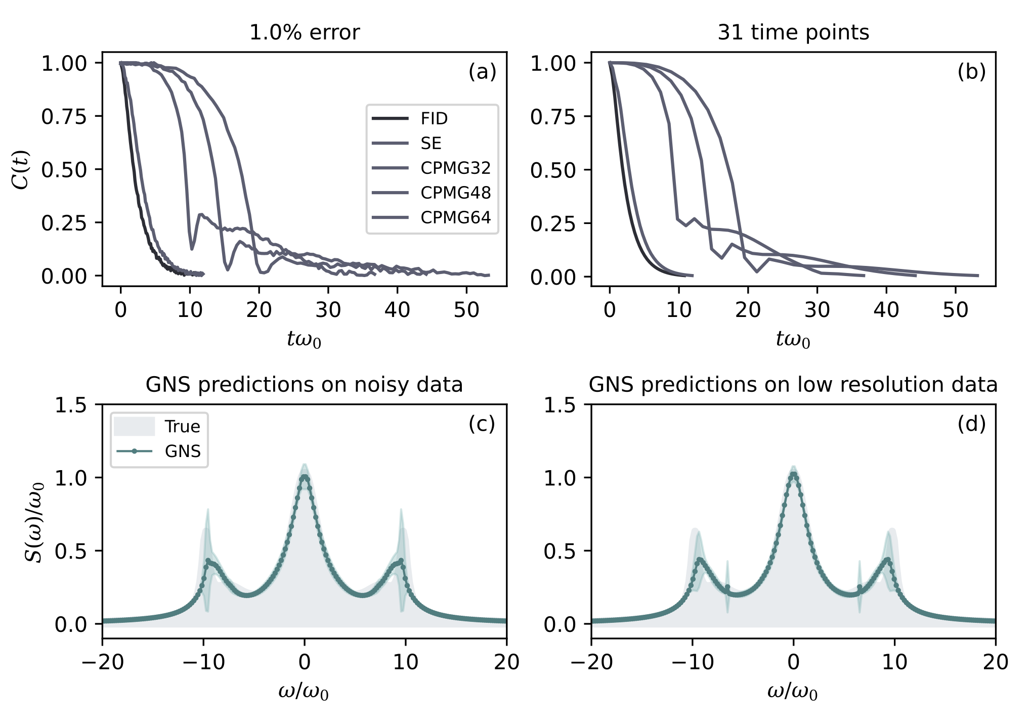
Figure 10: (a) Simulated FID, SE, CPMG32, CPMG48, and CPMG64 coherence measurements with an added 1.0% simulated uncorrelated noise, and (c) GNS predictions using these as input. For these data, we used a loss threshold of $\xi=8\times 10^{-4}$, $N_{\rm basis}=3$, and $N_{\rm runs}=20$. (b) Simulated FID, SE, CPMG32, CPMG48, and CPMG64 coherence measurements with decreased temporal resolution (31 total measurement points) and (d) GNS predictions using these as input. For these data, we employed a loss threshold of $\xi=7\times 10^{-4}$, $N_{\rm basis}=3$, and $N_{\rm runs}=20$.

Statistical error in the input measurement significantly hinders the performance of FTNS while GNS demonstrates remarkable robustness. The FID FTNS reconstructions in Fig. 9(c) suffer more in the presence of this effective error, manifesting spurious oscillatory features that become especially prominent at higher frequencies. On the other hand, SE FTNS predicts the structure at intermediate frequencies, $\omega\in[2,8]\omega_{0}$, relatively well, but struggles to capture the structure of the zero-frequency peak and the high-frequency peaks of the reference spectrum. This observation aligns with the fact that the SE filter function is heavily suppressed at $\omega\rightarrow 0$. In contrast, GNS offers a more reliable reconstruction of the entire spectrum, correctly capturing the peak height and width of the low-frequency contribution and the presence of and approximate position of the high-frequency feature.

We now compare the performances of the FTNS methods and GNS for data with limited temporal resolution in the absence of experimental noise. In particular, as a consequence of the Fourier transformation, the temporal resolution of the measured coherence curves limits the maximum resolvable frequency accessible with FTNS. To test this, we reduce the temporal resolution of the coherence curves in Fig. 9(a) in the absence of added noise from 101 equally distributed time points to 31, keeping the initial and final measurement times fixed (Fig. 9(b)).

As before, FTNS performance worsens significantly with poorer resolution of the input signals while GNS remain largely unchanged. Figure 9(d) compares the noise spectrum reconstructions obtained from FID FTNS, SE FTNS, and GNS. Both FTNS methods encounter limits on the maximum resolvable frequency (vertical dotted lines) that render them insensitive to the high-frequency features at $\omega\approx\pm 8$ in the test spectrum. In contrast, since GNS relies on the variational construction of a trial spectrum from a physical Lorentizan basis, its performance does not suffer from sparse sampling of the coherence curve. At low frequencies, the agreement of the predictions with the true spectrum is equally good for FID FTNS and GNS, although FID FTNS is insensitive to the presence of the higher frequency peak and so the reconstructed spectrum becomes inaccurate as the frequency approaches the Fourier limits. SE FTNS again suffers due to the SE filter function being insensitive to the $\omega\rightarrow 0$ limit of the power spectrum. One may explain the underestimation of the high-frequency peak amplitudes across all methods, even in the absence of simulated measurement error, by noting that only the FID and SE coherence curves are used for spectrum reconstruction and their filter functions are most sensitive to low-frequency noise contributions. Despite underestimating the high-frequency peaks, GNS is the only method that captures them and reproduces the correct asymptotic behavior at large frequencies.

Another distinct advantage of GNS over FTNS is that one can improve the former’s reliability by adding more measurements under different pulse numbers whereas FTNS can not. To demonstrate this point, Figure 10 shows the results of applying GNS on the data used in Fig. 9, but with additional CPMG measurements with 32, 48, and 64 pulses. We see that incorporating these pulses improves the prediction of the high-frequency peaks in both the noisy and low-resolution data.

Thus, GNS is limited neither by maximum frequency constraints nor by the effects of the measurement error in input coherence curves. In addition, the ability of GNS to achieve this level of efficacy in spectrum prediction without the need for denoising procedures makes it a practical choice for analyzing experimental data.

References

- Hahn [1950] E. L. Hahn, Spin echoes, Phys. Rev. 80, 580 (1950).
- Carr and Purcell [1954] H. Y. Carr and E. M. Purcell, Effects of diffusion on free precession in nuclear magnetic resonance experiments, Phys. Rev. 94, 630 (1954).
- Meiboom and Gill [1958] S. Meiboom and D. Gill, Modified spin-echo method for measuring nuclear relaxation times, Review of Scientific Instruments 29, 688 (1958).
- Viola and Lloyd [1998] L. Viola and S. Lloyd, Dynamical suppression of decoherence in two-state quantum systems, Physical Review A 58, 2733 (1998).
- Viola et al. [1999] L. Viola, E. Knill, and S. Lloyd, Dynamical decoupling of open quantum systems, Physical Review Letters 82, 2417 (1999).
- Vitali and Tombesi [1999] D. Vitali and P. Tombesi, Using parity kicks for decoherence control, Physical Review A 59, 4178 (1999).
- de Lange et al. [2010] G. de Lange, Z. H. Wang, D. Ristè, V. V. Dobrovitski, and R. Hanson, Universal dynamical decoupling of a single solid-state spin from a spin bath, Science 330, 60 (2010).
- Du et al. [2009] J. Du, X. Rong, N. Zhao, Y. Wang, J. Yang, and R. B. Liu, Preserving electron spin coherence in solids by optimal dynamical decoupling, Nature 461, 1265 (2009).
- Moisanu et al. [2024] C. M. Moisanu, H. J. Eckvahl, C. L. Stern, M. R. Wasielewski, and W. R. Dichtel, A paired-ion framework composed of vanadyl porphyrin molecular qubits extends spin coherence times, Journal of the American Chemical Society 146, 27975 (2024).
- Jiang et al. [2023] Z. Jiang, H. Cai, R. Cernansky, X. Liu, and W. Gao, Quantum sensing of radio-frequency signal with nv centers in sic, Science Advances 9 (2023).
- Jerger et al. [2023] P. C. Jerger, Y. X. Wang, M. Onizhuk, B. S. Soloway, M. T. Solomon, C. Egerstrom, F. J. Heremans, G. Galli, A. A. Clerk, and D. D. Awschalom, Detecting spin-bath polarization with quantum quench phase shifts of single spins in diamond, PRX Quantum 4, 10.1103/PRXQuantum.4.040315 (2023).
- Machado et al. [2023] F. Machado, E. A. Demler, N. Y. Yao, and S. Chatterjee, Quantum noise spectroscopy of dynamical critical phenomena, Physical Review Letters 131, 10.1103/PhysRevLett.131.070801 (2023).
- Müller et al. [2014] C. Müller, X. Kong, J. M. Cai, K. MelentijeviÄ, A. Stacey, M. Markham, D. Twitchen, J. Isoya, S. Pezzagna, J. Meijer, J. F. Du, M. B. Plenio, B. Naydenov, L. P. McGuinness, and F. Jelezko, Nuclear magnetic resonance spectroscopy with single spin sensitivity, Nature Communications 5, 10.1038/ncomms5703 (2014).
- Ajoy et al. [2015] A. Ajoy, U. Bissbort, M. D. Lukin, R. L. Walsworth, and P. Cappellaro, Atomic-scale nuclear spin imaging using quantum-assisted sensors in diamond, Physical Review X 5, 10.1103/PhysRevX.5.011001 (2015).
- Shi et al. [2015] F. Shi, Q. Zhang, P. Wang, H. Sun, J. Wang, X. Rong, M. Chen, C. Ju, F. Reinhard, H. Chen, J. Wrachtrup, J. Wang, and J. Du, Single-protein spin resonance spectroscopy under ambient conditions, Science 347, 1135 (2015).
- Lovchinsky et al. [2016] I. Lovchinsky, A. O. Sushkov, E. Urbach, N. P. de Leon, S. Choi, K. D. Greve, R. Evans, R. Gertner, E. Bersin, C. Müller, L. McGuinness, F. Jelezko, R. L. Walsworth, H. Park, and M. D. Lukin, Nuclear magnetic resonance detection and spectroscopy of single proteins using quantum logic, Science 351, 836 (2016).
- Shi et al. [2018] F. Shi, F. Kong, P. Zhao, X. Zhang, M. Chen, S. Chen, Q. Zhang, M. Wang, X. Ye, Z. Wang, Z. Qin, X. Rong, J. Su, P. Wang, P. Z. Qin, and J. Du, Single-dna electron spin resonance spectroscopy in aqueous solutions, Nature Methods 15, 697 (2018).
- Jenkins et al. [2019] A. Jenkins, M. Pelliccione, G. Yu, X. Ma, X. Li, K. L. Wang, and A. C. Jayich, Single-spin sensing of domain-wall structure and dynamics in a thin-film skyrmion host, Physical Review Materials 3, 10.1103/PhysRevMaterials.3.083801 (2019).
- Dovzhenko et al. [2018] Y. Dovzhenko, F. Casola, S. Schlotter, T. X. Zhou, F. Büttner, R. L. Walsworth, G. S. Beach, and A. Yacoby, Magnetostatic twists in room-temperature skyrmions explored by nitrogen-vacancy center spin texture reconstruction, Nature Communications 9, 10.1038/s41467-018-05158-9 (2018).
- Smits et al. [2019] J. Smits, J. T. Damron, P. Kehayias, A. F. McDowell, N. Mosavian, I. Fescenko, N. Ristoff, A. Laraoui, A. Jarmola, and V. M. Acosta, Two-dimensional nuclear magnetic resonance spectroscopy with a microfluidic diamond quantum sensor, Science Advances 5, eaaw7895 (2019), https://www.science.org/doi/pdf/10.1126/sciadv.aaw7895 .
- Abobeih et al. [2019] M. H. Abobeih, J. Randall, C. E. Bradley, H. P. Bartling, M. A. Bakker, M. J. Degen, M. Markham, D. J. Twitchen, and T. H. Taminiau, Atomic-scale imaging of a 27-nuclear-spin cluster using a quantum sensor, Nature 576, 411 (2019).
- Du et al. [2024] J. Du, F. Shi, X. Kong, F. Jelezko, and J. Wrachtrup, Single-molecule scale magnetic resonance spectroscopy using quantum diamond sensors, Reviews of Modern Physics 96, 10.1103/RevModPhys.96.025001 (2024).
- Degen et al. [2017] C. L. Degen, F. Reinhard, and P. Cappellaro, Quantum sensing, Reviews of Modern Physics 89, 10.1103/RevModPhys.89.035002 (2017).
- Zhao et al. [2012] N. Zhao, J. Honert, B. Schmid, M. Klas, J. Isoya, M. Markham, D. Twitchen, F. Jelezko, R. B. Liu, H. Fedder, and J. Wrachtrup, Sensing single remote nuclear spins, Nature Nanotechnology 7, 657 (2012).
- Dolde et al. [2011] F. Dolde, H. Fedder, M. W. Doherty, T. Nöbauer, F. Rempp, G. Balasubramanian, T. Wolf, F. Reinhard, L. C. Hollenberg, F. Jelezko, and J. Wrachtrup, Electric-field sensing using single diamond spins, Nature Physics 7, 459 (2011).
- Ovartchaiyapong et al. [2014] P. Ovartchaiyapong, K. W. Lee, B. A. Myers, and A. C. Jayich, Dynamic strain-mediated coupling of a single diamond spin to a mechanical resonator, Nature Communications 5, 10.1038/ncomms5429 (2014).
- Paz-Silva et al. [2017] G. A. Paz-Silva, L. M. Norris, and L. Viola, Multiqubit spectroscopy of gaussian quantum noise, Phys. Rev. A 95, 022121 (2017).
- Kwiatkowski et al. [2020] D. Kwiatkowski, P. Szańkowski, and L. Cywiński, Influence of nuclear spin polarization on the spin-echo signal of an nv-center qubit, Phys. Rev. B 101, 155412 (2020).
- Mukamel [1985] S. Mukamel, Fluorescence and absorption of large anharmonic molecules - spectroscopy without eigenstates, The Journal of Physical Chemistry 89, 1077 (1985), https://doi.org/10.1021/j100253a008 .
- Mukamel [1995] S. Mukamel, Principles of Nonlinear Optical Spectroscopy, Oxford Series in Optical and Imaging Sciences, Vol. 6 (Oxford University Press, 1995).
- Biercuk et al. [2011] M. J. Biercuk, A. C. Doherty, and H. Uys, Dynamical decoupling sequence construction as a filter-design problem, Journal of Physics B: Atomic, Molecular and Optical Physics 44, 10.1088/0953-4075/44/15/154002 (2011).
- Álvarez and Suter [2011] G. A. Álvarez and D. Suter, Measuring the spectrum of colored noise by dynamical decoupling, Physical Review Letters 107, 10.1103/PhysRevLett.107.230501 (2011).
- Bylander et al. [2011] J. Bylander, S. Gustavsson, F. Yan, F. Yoshihara, K. Harrabi, G. Fitch, D. G. Cory, Y. Nakamura, J. S. Tsai, and W. D. Oliver, Noise spectroscopy through dynamical decoupling with a superconducting flux qubit, Nature Physics 7, 565 (2011).
- Soetbeer et al. [2021] J. Soetbeer, L. F. Ibáñez, Z. Berkson, Y. Polyhach, and G. Jeschke, Regularized dynamical decoupling noise spectroscopy-a decoherence descriptor for radicals in glassy matrices, Physical Chemistry Chemical Physics 23, 21664 (2021).
- Chalermpusitarak et al. [2021] T. Chalermpusitarak, B. Tonekaboni, Y. Wang, L. M. Norris, L. Viola, and G. A. Paz-Silva, Frame-based filter-function formalism for quantum characterization and control, PRX Quantum 2, 10.1103/PRXQuantum.2.030315 (2021).
- Norris et al. [2016] L. M. Norris, G. A. Paz-Silva, and L. Viola, Qubit noise spectroscopy for non-gaussian dephasing environments, Physical Review Letters 116, 10.1103/PhysRevLett.116.150503 (2016).
- Sun and Cappellaro [2022] W. K. C. Sun and P. Cappellaro, Self-consistent noise characterization of quantum devices, Physical Review B 106, 10.1103/PhysRevB.106.155413 (2022).
- Lüpke et al. [2020] U. V. Lüpke, F. Beaudoin, L. M. Norris, Y. Sung, R. Winik, J. Y. Qiu, M. Kjaergaard, D. Kim, J. Yoder, S. Gustavsson, L. Viola, and W. D. Oliver, Two-qubit spectroscopy of spatiotemporally correlated quantum noise in superconducting qubits, PRX Quantum 1, 10.1103/PRXQuantum.1.010305 (2020).
- Tripathi et al. [2024] V. Tripathi, H. Chen, E. Levenson-Falk, and D. A. Lidar, Modeling low- and high-frequency noise in transmon qubits with resource-efficient measurement, PRX Quantum 5, 10.1103/PRXQuantum.5.010320 (2024).
- Wang et al. [2024] G. Wang, Y. Zhu, B. Li, C. Li, L. Viola, A. Cooper, and P. Cappellaro, Digital noise spectroscopy with a quantum sensor, Quantum Science and Technology 9, 10.1088/2058-9565/ad3846 (2024).
- Sung et al. [2021] Y. Sung, A. Vepsäläinen, J. Braumüller, F. Yan, J. I. Wang, M. Kjaergaard, R. Winik, P. Krantz, A. Bengtsson, A. J. Melville, B. M. Niedzielski, M. E. Schwartz, D. K. Kim, J. L. Yoder, T. P. Orlando, S. Gustavsson, and W. D. Oliver, Multi-level quantum noise spectroscopy, Nature Communications 12, 10.1038/s41467-021-21098-3 (2021).
- Wudarski et al. [2023] F. Wudarski, Y. Zhang, A. N. Korotkov, A. G. Petukhov, and M. I. Dykman, Characterizing low-frequency qubit noise, Physical Review Applied 19, 10.1103/PhysRevApplied.19.064066 (2023).
- Rovny et al. [2022] J. Rovny, Z. Yuan, M. Fitzpatrick, A. I. Abdalla, L. Futamura, C. Fox, M. C. Cambria, S. Kolkowitz, and N. P. de Leon, Nanoscale covariance magnetometry with diamond quantum sensors, Science 378, 1301 (2022).
- Paz-Silva et al. [2019] G. A. Paz-Silva, L. M. Norris, F. Beaudoin, and L. Viola, Extending comb-based spectral estimation to multiaxis quantum noise, Physical Review A 100, 10.1103/PhysRevA.100.042334 (2019).
- Khan et al. [2024] M. Q. Khan, W. Dong, L. M. Norris, and L. Viola, Multiaxis quantum noise spectroscopy robust to errors in state preparation and measurement, Physical Review Applied 22, 10.1103/PhysRevApplied.22.024074 (2024).
- Sangtawesin et al. [2019] S. Sangtawesin, B. L. Dwyer, S. Srinivasan, J. J. Allred, L. V. Rodgers, K. D. Greve, A. Stacey, N. Dontschuk, K. M. O’Donnell, D. Hu, D. A. Evans, C. Jaye, D. A. Fischer, M. L. Markham, D. J. Twitchen, H. Park, M. D. Lukin, and N. P. D. Leon, Origins of diamond surface noise probed by correlating single-spin measurements with surface spectroscopy, Physical Review X 9, 10.1103/PhysRevX.9.031052 (2019).
- Monge et al. [2023] R. Monge, T. Delord, N. V. Proscia, Z. Shotan, H. Jayakumar, J. Henshaw, P. R. Zangara, A. Lozovoi, D. Pagliero, P. D. Esquinazi, T. An, I. Sodemann, V. M. Menon, and C. A. Meriles, Spin dynamics of a solid-state qubit in proximity to a superconductor, Nano Letters 23, 422 (2023).
- Chrostoski et al. [2022] P. Chrostoski, P. Kehayias, and D. H. Santamore, Surface roughness noise analysis and comprehensive noise effects on depth-dependent coherence time of nv centers in diamond, Physical Review B 106, 10.1103/PhysRevB.106.235311 (2022).
- Myers et al. [2014] B. A. Myers, A. Das, M. C. Dartiailh, K. Ohno, D. D. Awschalom, and A. C. B. Jayich, Probing surface noise with depth-calibrated spins in diamond, Physical Review Letters 113, 10.1103/PhysRevLett.113.027602 (2014).
- Dial et al. [2013] O. E. Dial, M. D. Shulman, S. P. Harvey, H. Bluhm, V. Umansky, and A. Yacoby, Charge noise spectroscopy using coherent exchange oscillations in a singlet-triplet qubit, Physical Review Letters 110, 10.1103/PhysRevLett.110.146804 (2013).
- Barr et al. [2024] J. Barr, G. Zicari, A. Ferraro, and M. Paternostro, Spectral density classification for environment spectroscopy, Machine Learning: Science and Technology 5, 10.1088/2632-2153/ad2cf1 (2024).
- Malinowski et al. [2017] F. K. Malinowski, F. Martins, Łukasz Cywiński, M. S. Rudner, P. D. Nissen, S. Fallahi, G. C. Gardner, M. J. Manfra, C. M. Marcus, and F. Kuemmeth, Spectrum of the nuclear environment for gaas spin qubits, Physical Review Letters 118, 10.1103/PhysRevLett.118.177702 (2017).
- Bar-Gill et al. [2012] N. Bar-Gill, L. M. Pham, C. Belthangady, D. L. Sage, P. Cappellaro, J. R. Maze, M. D. Lukin, A. Yacoby, and R. Walsworth, Suppression of spin-bath dynamics for improved coherence of multi-spin-qubit systems, Nature Communications 3, 10.1038/ncomms1856 (2012).
- Romach et al. [2015] Y. Romach, C. Müller, T. Unden, L. J. Rogers, T. Isoda, K. M. Itoh, M. Markham, A. Stacey, J. Meijer, S. Pezzagna, B. Naydenov, L. P. McGuinness, N. Bar-Gill, and F. Jelezko, Spectroscopy of surface-induced noise using shallow spins in diamond, Physical Review Letters 114, 10.1103/PhysRevLett.114.017601 (2015).
- Biercuk et al. [2009] M. J. Biercuk, H. Uys, A. P. Vandevender, N. Shiga, W. M. Itano, and J. J. Bollinger, Experimental uhrig dynamical decoupling using trapped ions, Physical Review A - Atomic, Molecular, and Optical Physics 79, 10.1103/PhysRevA.79.062324 (2009).
- Connors et al. [2022] E. J. Connors, J. Nelson, L. F. Edge, and J. M. Nichol, Charge-noise spectroscopy of si/sige quantum dots via dynamically-decoupled exchange oscillations, Nature Communications 13, 10.1038/s41467-022-28519-x (2022).
- Muhonen et al. [2014] J. T. Muhonen, J. P. Dehollain, A. Laucht, F. E. Hudson, R. Kalra, T. Sekiguchi, K. M. Itoh, D. N. Jamieson, J. C. McCallum, A. S. Dzurak, and A. Morello, Storing quantum information for 30 seconds in a nanoelectronic device, Nature Nanotechnology 9, 986 (2014).
- Medford et al. [2012] J. Medford, A. Cywiński, C. Barthel, C. M. Marcus, M. P. Hanson, and A. C. Gossard, Scaling of dynamical decoupling for spin qubits, Physical Review Letters 108, 10.1103/PhysRevLett.108.086802 (2012).
- Oliveira et al. [2017] F. F. D. Oliveira, D. Antonov, Y. Wang, P. Neumann, S. A. Momenzadeh, T. Häußermann, A. Pasquarelli, A. Denisenko, and J. Wrachtrup, Tailoring spin defects in diamond by lattice charging, Nature Communications 8, 10.1038/ncomms15409 (2017).
- Kim et al. [2015] M. Kim, H. J. Mamin, M. H. Sherwood, K. Ohno, D. D. Awschalom, and D. Rugar, Decoherence of near-surface nitrogen-vacancy centers due to electric field noise, Physical Review Letters 115, 10.1103/PhysRevLett.115.087602 (2015).
- Ishizu et al. [2020] S. Ishizu, K. Sasaki, D. Misonou, T. Teraji, K. M. Itoh, and E. Abe, Spin coherence and depths of single nitrogen-vacancy centers created by ion implantation into diamond via screening masks, Journal of Applied Physics 127, 10.1063/5.0012187 (2020).
- Vezvaee et al. [2024] A. Vezvaee, N. Shitara, S. Sun, and A. Montoya-Castillo, Fourier transform noise spectroscopy, npj Quantum Information 10, 10.1038/s41534-024-00841-w (2024).
- Pezzagna and Meijer [2021] S. Pezzagna and J. Meijer, Quantum computer based on color centers in diamond, Applied Physics Reviews 8, 10.1063/5.0007444 (2021).
- Harty et al. [2014] T. P. Harty, D. T. Allcock, C. J. Ballance, L. Guidoni, H. A. Janacek, N. M. Linke, D. N. Stacey, and D. M. Lucas, High-fidelity preparation, gates, memory, and readout of a trapped-ion quantum bit, Physical Review Letters 113, 10.1103/PhysRevLett.113.220501 (2014).
- Graham et al. [2022] T. M. Graham, Y. Song, J. Scott, C. Poole, L. Phuttitarn, K. Jooya, P. Eichler, X. Jiang, A. Marra, B. Grinkemeyer, M. Kwon, M. Ebert, J. Cherek, M. T. Lichtman, M. Gillette, J. Gilbert, D. Bowman, T. Ballance, C. Campbell, E. D. Dahl, O. Crawford, N. S. Blunt, B. Rogers, T. Noel, and M. Saffman, Multi-qubit entanglement and algorithms on a neutral-atom quantum computer, Nature 604, 457 (2022).
- Wintersperger et al. [2023] K. Wintersperger, F. Dommert, T. Ehmer, A. Hoursanov, J. Klepsch, W. Mauerer, G. Reuber, T. Strohm, M. Yin, and S. Luber, Neutral atom quantum computing hardware: performance and end-user perspective, EPJ Quantum Technology 10, 10.1140/epjqt/s40507-023-00190-1 (2023).
- Kingma and Ba [2014] D. P. Kingma and J. Ba, Adam: A method for stochastic optimization (2014), arXiv:1412.6980 [cs.LG] .
- Paladino et al. [2014] E. Paladino, Y. M. Galperin, G. Falci, and B. L. Altshuler, noise: Implications for solid-state quantum information, Rev. Mod. Phys. 86, 361 (2014).
- Szańkowski et al. [2017] P. Szańkowski, G. Ramon, J. Krzywda, D. Kwiatkowski, and Cywiński, Environmental noise spectroscopy with qubits subjected to dynamical decoupling, Journal of Physics Condensed Matter 29, 10.1088/1361-648X/aa7648 (2017).
- Uhrig [2007] G. S. Uhrig, Keeping a quantum bit alive by optimized -pulse sequences, Physical Review Letters 98, 100504 (2007).
- Uhrig [2008] G. S. Uhrig, Exact results on dynamical decoupling by pulses in quantum information processes, New Journal of Physics 10, 083024 (2008).
- Łukasz Cywiński et al. [2008] Łukasz Cywiński, R. M. Lutchyn, C. P. Nave, and S. D. Sarma, How to enhance dephasing time in superconducting qubits, Physical Review B 77, 174509 (2008).
- Szańkowski and Łukasz Cywiński [2018] P. Szańkowski and Łukasz Cywiński, Accuracy of dynamical-decoupling-based spectroscopy of gaussian noise, Physical Review A 97, 10.1103/PhysRevA.97.032101 (2018).
- Karniadakis and Sherwin [2005] G. Karniadakis and S. J. Sherwin, Spectral/hp element methods for computational fluid dynamics (Oxford University Press, USA, 2005).
- Boyd [2001] J. P. Boyd, Chebyshev and Fourier spectral methods (Courier Corporation, 2001).
- Klauder and Anderson [1962] J. R. Klauder and P. W. Anderson, Spectral diffusion decay in spin resonance experiments, Physical Review 125, 912 (1962).
- Meier and Tannor [1999] C. Meier and D. J. Tannor, Non-markovian evolution of the density operator in the presence of strong laser fields, Journal of Chemical Physics 111, 3365 (1999).
- Liu et al. [2014] H. Liu, L. Zhu, S. Bai, and Q. Shi, Reduced quantum dynamics with arbitrary bath spectral densities: Hierarchical equations of motion based on several different bath decomposition schemes, Journal of Chemical Physics 140, 10.1063/1.4870035 (2014).
- Dirdal and Skaar [2013] C. A. Dirdal and J. Skaar, Superpositions of lorentzians as the class of causal functions, Physical Review A - Atomic, Molecular, and Optical Physics 88, 10.1103/PhysRevA.88.033834 (2013).
- [80] Pytorch, https://pytorch.org/.
- [81] Tensorflow, https://www.tensorflow.org.
- Hong et al. [2013] S. Hong, M. S. Grinolds, L. M. Pham, D. L. Sage, L. Luan, R. L. Walsworth, and A. Yacoby, Nanoscale magnetometry with nv centers in diamond, MRS Bulletin 38, 155 (2013).
- Weierstrass [1885] K. Weierstrass, Uber die analytische darstellbarkeit sogenannter willkurlicher funktionen reeller argumente, SB Deutsche Akad. Wiss. Berlin KL. Math. Phys. Tech. (1885).
- Hernández-Gómez et al. [2018] S. Hernández-Gómez, F. Poggiali, P. Cappellaro, and N. Fabbri, Noise spectroscopy of a quantum-classical environment with a diamond qubit, Physical Review B 98, 10.1103/PhysRevB.98.214307 (2018).
- Loshchilov and Hutter [2017] I. Loshchilov and F. Hutter, Decoupled weight decay regularization (2017), arXiv:1711.05101 [cs.LG] .