Contrastive Graph Condensation: Advancing Data Versatility through Self-Supervised Learning

Abstract

With the increasing computation of training graph neural networks (GNNs) on large-scale graphs, graph condensation (GC) has emerged as a promising solution to synthesize a compact, substitute graph of the large-scale original graph for efficient GNN training. However, existing GC methods predominantly employ classification as the surrogate task for optimization, thus excessively relying on node labels and constraining their utility in label-sparsity scenarios. More critically, this surrogate task tends to overfit class-specific information within the condensed graph, consequently restricting the generalization capabilities of GC for other downstream tasks. To address these challenges, we introduce Contrastive Graph Condensation (CTGC), which adopts a self-supervised surrogate task to extract critical, causal information from the original graph and enhance the cross-task generalizability of the condensed graph. Specifically, CTGC employs a dual-branch framework to disentangle the generation of the node attributes and graph structures, where a dedicated structural branch is designed to explicitly encode geometric information through nodes’ positional embeddings. By implementing an alternating optimization scheme with contrastive loss terms, CTGC promotes the mutual enhancement of both branches and facilitates high-quality graph generation through the model inversion technique. Extensive experiments demonstrate that CTGC excels in handling various downstream tasks with a limited number of labels, consistently outperforming state-of-the-art GC methods.

I Introduction

Graph neural networks (GNNs) [1, 2, 3] have been widely employed across complex systems to analyze graph-structured data, including chemical molecules [4], social networks [5, 6], and recommender systems [7, 8]. However, the exponential increase in graph data volume presents formidable challenges for training GNNs, particularly in scenarios that necessitate training multiple models, such as neural architecture search [9], continual learning [10], and federated learning [11]. In addressing these challenges, graph condensation (GC) [12] has emerged as a promising approach. It synthesizes a compact yet representative condensed graph that serves as a substitute for the large-scale original graph during model training. By preserving the essential attributes of the original graph, GNNs trained on the condensed graph achieve performance comparable to those trained on the original graph while significantly reducing the training time and broadening their applicability in resource-constrained scenarios.

Due to their efficacy in accelerating model training processes, GC methods have attracted substantial attention and achieved significant progress. To synthesize condensed data, GC methods typically leverage a relay model to bridge the original and condensed graphs, deploying the classification as the surrogate task for optimization [13]. Initially, GC methods utilize sophisticated optimization strategies and focus on matching parameters of the classification relay model, including model gradients [12] and training trajectories [14] generated from both graphs. Subsequently, advanced studies expand these parameter matching methods to lighter label regression [15] and class-prototype matching [16], further enhancing the efficiency and effectiveness of the condensation process. Despite the diversity of existing GC approaches, the optimization processes in these methods consistently center on the classification surrogate task, and a recent study [17] highlights that all these methods converge to the class distribution matching between the original and condensed graphs. As a result, this uniform reliance on the classification surrogate task significantly constrains the real-world practicality of GC.

Specifically, the application of the classification surrogate task within GC optimization encounters two primary limitations. On the one hand, the efficacy of GC is critically dependent on label availability, with existing methods premised on the assumption of abundant labels [18]. Unfortunately, this assumption often contradicts real-world scenarios, where labels in large-scale graphs are costly to annotate and scarce [19]. This label scarcity leads to imprecise class representations, thereby diminishing the effectiveness of GC methods. On the other hand, the classification surrogate task in these methods tends to overfit class-specific information within the condensed graph, consequently restricting the capability of the condensed graph to support diverse downstream tasks [20]. As illustrated in Fig. 1, models trained on condensed graphs in the label sparsity setting consistently underperform those trained on the original graph, not only in node classification but also across other downstream tasks. In practice, downstream tasks vary significantly across real-world graph systems; for instance, recommendation systems model user-item interactions as link prediction tasks [21, 22], while clustering tasks are essential for analyzing item characteristics and user behaviors [23]. Therefore, it is imperative for GNNs trained on condensed graphs to demonstrate generalizability to a variety of downstream tasks within polytropic environments. In a nutshell, the critical problem that arises for GC is: “How can we effectively distill essential knowledge to the condensed graph without the dependency on class labels, and ensure the GNNs trained on condensed graphs maintain generalizability across diverse downstream tasks?”

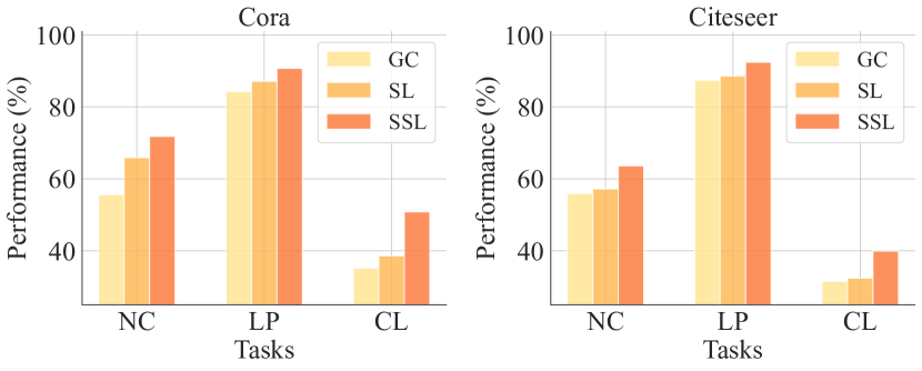
Figure 1: The performance of models trained on the condensed graph (GC) [12], the original graph with supervised learning (SL), and the original graph with our proposed self-supervised learning (SSL) task. The 3-shot setting is applied. Node classification (NC), link prediction (LP), and clustering (CL) are assessed using accuracy, AUC, and NMI, respectively.

To tackle this problem, self-supervised learning (SSL) [24, 25, 26] provides a promising direction, as it inherently enables the learning of more transferable and adaptable representations without label availability, addressing the task-specific bias introduced by the classification surrogate task. This effectiveness is illustrated in Fig. 1, where the model trained with the self-supervised task outperforms the supervised learning model across the three tasks under the label sparsity issue. Despite the potential of SSL to enhance task generalization, developing a self-supervised method for GC remains an open area, which meets three critical objectives: (1) the surrogate task should extract the representative yet task-invariant information from the original graph in a self-supervised manner to circumvent task-specific biases introduced by class labels; (2) it should effectively summarize and compress the extracted information to facilitate the generation of a condensed graph; and (3) instead of using pairwise similarity between condensed node attributes [12, 16], the condensed graph structure should be independently constructed [20, 27] to topologically mimic the original graph, so as to offer stronger supplement predictive signals when training a GNN for diverse tasks. Although a recent attempt [28] in graph-level dataset condensation tries to generate condensed graphs from any pre-trained GNN model, this method fails to handle the node-level tasks, and the arbitrary selection of a pre-trained model may not represent the ideal distribution for effective GC, potentially compromising the practical utility of the condensed graph.

In response to these objectives, we propose Contrastive Graph Condensation (CTGC), a self-supervised GC approach designed to efficiently handle diverse downstream tasks. As illustrated in Fig. 2, CTGC utilizes a dual-branch framework composed of semantic and structural branches, which are iteratively optimized through a unified contrastive surrogate task. Specifically, the semantic branch processes node attributes according to the graph structure to extract latent semantic information, while the structural branch explicitly encodes geometric information using the eigenvectors of the graph structure. These branches are optimized through contrastive losses, encouraging intra-cluster proximity and inter-cluster separability. Moreover, to promote mutual enhancement and alignment between branches, we propose an alternating optimization framework to optimize two branches iteratively with the exchange of cluster assignments. Subsequently, the centroid embeddings from the two branches can be utilized to recover the node attributes and topological structures of the condensed graph through the model inversion technique [29, 30], respectively. Consequently, CTGC eliminates the dependence on class labels in the condensation procedure and enables the independent generation of graph structures, thus facilitating high-quality condensed graphs and improving cross-task generalizability.

The main contributions of this paper are threefold:

• New observations and insights. We identify the limitation of the classification surrogate task as a bottleneck for label dependency and task generalization in existing GC. This emphasizes the necessity of designing a self-supervised surrogate task, which significantly broadens potential applications of GC in real-world scenarios.

• New methodology. We present CTGC, a self-supervised GC method characterized by a novel dual-branch framework and a contrastive surrogate task. The semantic and structural information are disengaged in two branches, while the contrastive task enables extracting transferrable information for condensation, enhancing the cross-task generalizability of GC.

• State-of-the-art performance. Extensive experiments verify that CTGC excels in generating high-quality condensed graphs without label availability, surpassing various state-of-the-art GC methods in performance.

II Preliminaries

In this section, we first revisit the fundamental concepts of GNNs, eigenvalue decomposition, and GC, and then formally define the problem studied.

II-A Graph Neural Networks

Consider that we have a large-scale graph $\mathcal{T}=\{{\bf A},{\bf X}\}$ consisting of $N$ nodes. ${\bf X}\in{\mathbb{R}^{N\times d}}$ denotes the $d$-dimensional node attribute matrix and ${\bf A}\in\mathbb{R}^{N\times N}$ is the adjacency matrix. We use ${\bf Y}\in{\mathbb{R}^{N\times C}}$ to denote the one-hot node labels over $C$ classes. GNNs learn the embedding for each node by leveraging the graph structure and node attribute as the input. Without loss of generality, we use graph convolutional network (GCN) [31] as an example, where the convolution operation in the $k$-th layer is defined as follows:

$${\bf{H}}^{(k)}=\text{ReLU}\left(\hat{\mathbf{A}}{\bf H}^{(k-1)}{\mathbf{W}}^{(k)}\right),$$ (1)

where ${\bf{H}}^{(k)}$ is the node embeddings of the $k$-th layer, and ${\bf{H}}^{(0)}=\mathbf{X}$. $\hat{\mathbf{A}}=\widetilde{\mathbf{D}}^{-\frac{1}{2}}\widetilde{\mathbf{A}}\widetilde{\mathbf{D}}^{-\frac{1}{2}}$ is the normalized adjacency matrix. $\widetilde{\mathbf{A}}$ represents the adjacency matrix with the self-loop, $\widetilde{\mathbf{D}}$ denotes the degree matrix of $\widetilde{\mathbf{A}}$, and $\mathbf{W}^{(k)}$ is the trainable weights. $\text{ReLU}\left(\cdot\right)$ is the rectified linear unit function. Afterward, the $K$-th layer embeddings ${\bf{H}}^{(K)}$ are predicted by specific prediction heads for different downstream tasks.

II-B Eigenvalue Decomposition

Given the adjacency matrix ${\bf A}$, the normalized graph Laplacian is defined as ${\mathbf{L}}={\mathbf{I}}-{\mathbf{D}}^{-\frac{1}{2}}{\mathbf{A}}{\mathbf{D}}^{-\frac{1}{2}}$, where ${\mathbf{I}}$ is the identity matrix. The eigenvalue decomposition of graph Laplacian is defined as ${\mathbf{L}}={\bf U}{\bf{\Lambda}}{\bf U}^{\top}$, where ${\top}$ denotes the transpose operation. ${\bf{\Lambda}}$ is a diagonal matrix whose diagonal entries $0\leq\lambda_{1}\leq...\leq\lambda_{N}\leq 2$ are the eigenvalues of ${\mathbf{L}}$. ${\bf U}=[{\bf u}_{1},...,{\bf u}_{N}]\in\mathbb{R}^{N\times N}$ are the corresponding eigenvectors.

The eigenvalues and eigenvectors encapsulate the geometric information and node positions within the graph topology, providing a comprehensive view of graph structural information. Specifically, the eigenvalues [32] summarize key structural properties, such as connectivity [33], clusterability [34], and diffusion distance [35]. Meanwhile, the eigenvectors in ${\bf U}$ serve as positional embeddings [36, 37], capturing the local structure associated with each node [38].

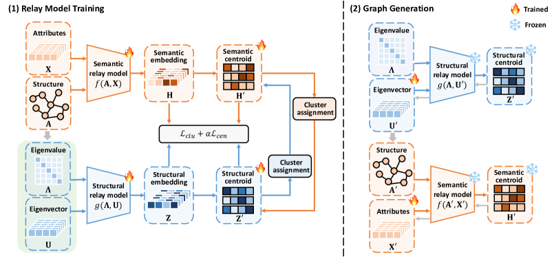
Figure 2: The framework of our proposed CTGC, which comprises two stages: relay model training and graph generation. (1) CTGC employs a dual-branch architecture to separately extract semantic and structural information. The semantic relay model processes both the graph structure and node attributes, while the structural relay model uses eigenvalues and eigenvectors as inputs. These branches are iteratively optimized using contrastive losses. (2) The condensed graph is generated using the model inversion technique. This process begins with generating eigenvectors to construct the condensed graph structure, followed by learning node attributes based on the constructed graph structure.

II-C Graph Condensation

Conventional graph condensation methods [12] are primarily developed within a supervised framework, aiming to generate a small condensed graph $\mathcal{S}=\{{\bf A^{\prime}},{\bf X^{\prime}}\}$ with ${\bf A^{\prime}}\in\mathbb{R}^{N^{\prime}\times N^{\prime}}$, ${\bf X^{\prime}}\in\mathbb{R}^{N^{\prime}\times d}$ as well as its label ${\bf Y^{\prime}}\in{\mathbb{R}^{N^{\prime}\times C}}$, where $N^{\prime}\ll{N}$. The condensation ratio is denoted as $r=\frac{N^{\prime}}{N}$. GNNs trained on $\mathcal{S}$ can achieve comparable performance to those trained on the much larger $\mathcal{T}$. To connect the original graph $\mathcal{T}$ and condensed graph $\mathcal{S}$, a relay model $f_{\theta}$ parameterized by ${\theta}$ is employed in GC for encoding both graphs. Concurrently, a surrogate task is introduced within the condensation process to facilitate the optimization of the relay model and the condensed graph. Specifically, the classification task is predominantly employed as the surrogate task in existing GC methods, and the classification losses of $\mathcal{T}$ and $\mathcal{S}$ w.r.t. ${\theta}$ are defined as:

$$\begin{split}&\mathcal{L}\left(\theta\right)=\ell\left(f_{\theta}\left({\mathcal{T}}\right),\mathbf{Y}\right),\\ &\mathcal{L}^{\prime}\left(\theta\right)=\ell\left(f_{\theta}\left({\mathcal{S}}\right),\mathbf{Y}^{\prime}\right),\end{split}$$ (2)

where $\ell\left(\cdot,\cdot\right)$ is the cross-entropy loss and $\mathbf{Y}^{\prime}$ is predefined to match the class distribution in $\mathbf{Y}$. Then the objective of GC can be formulated as a bi-level optimization problem:

$$\min_{\mathcal{S}}\mathcal{L}\left(\theta^{\mathcal{S}}\right)\>\>\text{s.t.}\>\>\theta^{\mathcal{S}}=\arg\min_{\mathcal{\theta}}\mathcal{L}^{\prime}\left(\theta\right).$$ (3)

To solve this objective, the typical GC method [12] proposes to align the model gradients at each training step $t$ generated from two graphs. This approach allows the training trajectory on the condensed graph to mimic that of the original training graph, ensuring that models trained on both graphs converge to comparable solutions. The objective is defined as:

$$\begin{split}&\mathcal{L}_{cond}=\min_{\mathcal{S}}\mathbb{E}_{\theta_{0}\sim{\Theta}}\left[\sum_{t=1}^{T}\mathcal{D}\left(\nabla_{\theta_{t}}\mathcal{L}\left({\theta_{t}}\right),\nabla_{\theta_{t}}\mathcal{L}^{\prime}\left({\theta_{t}}\right)\right)\right]\,\,\\ &\text{s.t.}\,\,{\theta}_{t+1}=\operatorname{opt}\left(\mathcal{L}^{\prime}\left({\theta_{t}}\right)\right),\end{split}$$ (4)

where $\theta_{0}$ denotes the initial parameters of the relay model, which is sampled from the distribution ${\Theta}$. The expectation on $\theta_{0}$ aims to improve the robustness of ${\mathcal{S}}$ to different parameter initialization [39]. $\operatorname{opt}\left(\cdot\right)$ is the model optimizer and the relay model is updated only on $\mathcal{S}$. $\mathcal{D}\left(\cdot,\cdot\right)$ is the distance measurement to calculate the gradient distances. Suppose the gradient $\nabla_{\theta}\mathcal{L}=\{\mathbf{G}^{(p)}\}_{p=1}^{P}$ and $\nabla_{\theta}\mathcal{L}^{\prime}=\{\mathbf{G}^{\prime(p)}\}_{p=1}^{P}$ in Eq. (4) entails all $P$ layers’ model gradient matrices $\mathbf{G}^{(p)}$ and $\mathbf{G}^{\prime(p)}$, $\mathcal{D}\left(\cdot,\cdot\right)$ is calculated by summing up all layers’ pairwise gradient distances:

$$\mathcal{D}(\nabla_{\theta}\mathcal{L},\nabla_{\theta}\mathcal{L}^{\prime})=\sum_{p=1}^{P}\sum_{i=1}^{D_{p}}\left(1-\text{sim}\left(\mathbf{G}^{(p)}_{i},{\mathbf{G}^{\prime}_{i}}^{(p)}\right)\right),$$ (5)

where $\text{sim}(\cdot,\cdot)$ is the cosine similarity, $\mathbf{G}^{(p)}_{i}$ and $\mathbf{G}^{\prime(p)}_{i}$ are the $i$-th column vector in the gradient matrix $\mathbf{G}^{(p)}$ and $\mathbf{G}^{\prime(p)}$ at layer $p$, respectively.

Notice that, to simplify the optimization of the structure of condensed graph, typical GC methods [12, 40] entangle the graph structure with the node attributes, parameterizing $\mathbf{A}^{\prime}$ by $\mathbf{X}^{\prime}$ as:

$${\bf A}_{i,j}^{\prime}=\sigma\left(\frac{{\text{MLP}([{\bf X}^{\prime}_{i};{\bf X}^{\prime}_{j}])}+{\text{MLP}([{\bf X}^{\prime}_{j};{\bf X}^{\prime}_{i}])}}{2}\right),$$ (6)

where $\text{MLP}(\cdot)$ is a multi-layer perceptron (MLP), and fed with the concatenation of condensed node features ${\bf X}^{\prime}_{i}$ and ${\bf X}^{\prime}_{j}$. $\sigma$ denotes the sigmoid function.

In addition to gradient matching, various GC methods employ diverse optimization strategies to address the objective in Eq. (3), including distribution matching [16, 27], trajectory matching [14] and kernel ridge regression [15]. While these methods demonstrate the potential to improve GC performance, they all deploy the classification as the surrogate task, which inherently impacts the cross-task generalizability of GC.

II-D Problem Formulation

To mitigate the dependency on labels within the GC, we focus on a self-supervised GC framework targeting a large unlabeled graph $\mathcal{T}=\{\mathbf{A},\mathbf{X}\}$. Our objective is to generate a small condensed graph $\mathcal{S}=\{{\bf A^{\prime}},{\bf X^{\prime}}\}$ with $d$-dimensional target embeddings ${\bf H}^{\prime}\in{\mathbb{R}^{N^{\prime}\times d}}$, which serve as proxy labels of $\mathcal{S}$ to facilitate the pre-training of downstream GNNs. This condensed graph $\mathcal{S}$ expedites the model pre-training processes, allowing the pre-trained model to be fine-tuned efficiently for adaptation across various downstream tasks.

III Methodologies

We hereby present our proposed method, Contrastive Graph Condensation (CTGC), which comprises two stages: relay model training and graph generation, as illustrated in Fig. 2. Initially, CTGC employs a dual-branch architecture to extract semantic and structural information separately. Then we move on to the contrastive surrogate task to optimize the semantic and structural relay models, as well as to develop the centroid embeddings. Finally, we generate the graph structure and node attributes using the relay models and centroid embeddings, culminating in the construction of the condensed graph.

III-A Dual-Branch Architecture

The conventional condensation procedure described in Section II-C employs a single relay model to encode both the graph structure information and the node attributes, with the structure of the condensed graph being generated based on condensed node attributes as Eq. (6). Although it simplifies the optimization of graph structure, the entanglement of condensed nodes and structure heavily caps the amount of preserved topological information from the original graph [20, 27]. To mitigate this limitation, we introduce an additional structural branch to generate graph structure from the spectral perspective.

Specifically, two distinct relay models are introduced to encode the original graph:

$$\begin{split}&{\bf{H}}=f({\bf A},{\bf X}),\\ &{\bf{Z}}=g({\bf{\Lambda}},{\bf U}),\end{split}$$ (7)

where $f(\cdot)$ and $g(\cdot)$ represent the relay models for the semantic and structural branches, respectively. $f(\cdot)$ is the GNN model as used in conventional GC methods, while $g(\cdot)$ processes the eigenvalues $\bf{\Lambda}$ and eigenvectors ${\bf U}$ to produce the structural embeddings ${\bf Z}\in\mathbb{R}^{N\times d}$ for the original graph. To facilitate scalable encoding, EigenMLP [41] is leveraged as the structural relay model $g(\cdot)$ as follows:

$$g({\bf{\Lambda}},{\bf U})={\tilde{\bf{U}}}\rho({\bf{\Lambda}}),$$ (8)

where ${\tilde{\bf{U}}}$ is the sign-invariant eigenvectors and $\rho({\bf{\Lambda}})$ represents the filtered eigenvalues. The implementation of EigenMLP mitigates the sign ambiguity and basis ambiguity [41] inherent in eigenvector decompositions, where arbitrary sign flips and coordinate rotations of eigenvectors can yield identical graph structures. Specifically, the sign-invariant eigenvectors are derived by taking both positive and negative forms of eigenvectors into consideration:

$${\tilde{\bf{U}}}=[\psi(\phi({\bf{u}}_{i})+\phi({\bf{-u}}_{i}))]_{i=1}^{N},$$ (9)

where $\psi(\cdot)$ and $\phi(\cdot)$ represent MLPs to transform the eigenvalues, and $[\cdot]$ denotes the concatenation operator. $[{\bf u}_{1},...,{\bf u}_{N}]\in\mathbb{R}^{N\times N}$ are eigenvectors. Additionally, $\rho({\bf{\Lambda}})$ extends the eigenvalues ${\bf{\Lambda}}=[\lambda_{1},\lambda_{2},...,\lambda_{N}]$ to their high-dimensional Fourier features to mitigate the bias ambiguity as:

$$\begin{split}&\rho({\bf{\Lambda}})=[\rho(\lambda_{1}),\rho(\lambda_{2}),...,\rho(\lambda_{N})]^{\top},\\ &\rho(\lambda)=[\sin(\lambda),\cos(\lambda),...,\sin(T\lambda),\cos(T\lambda)]{\bf W}_{\rho},\end{split}$$ (10)

where $T$ represents the period and ${\bf W}_{\rho}\in\mathbb{R}^{2T\times d}$ is a learnable weight matrix.

Although EigenMLP effectively models the graph structure from a spectral perspective, employing all eigenvectors is impractical due to the inclusion of the dense and large matrix ${\tilde{\bf{U}}}\in\mathbb{R}^{N\times N}$, resulting in significant computational and memory costs for large graphs. In practice, eigenvectors associated with the smallest and largest eigenvalues are critical for encapsulating geometric information. Eigenvectors corresponding to smaller eigenvalues emphasize the global community structure [32], while those associated with larger eigenvalues capture local features [37]. These crucial eigenvectors play a pivotal role in graph modeling and are widely utilized in spectral GNNs [42] and graph reduction methods [43, 27]. To mitigate the computational burden of complete eigenvalue decomposition, we follow prior work [27] by using the $K_{1}$ smallest and $K_{2}$ largest eigenvalues, along with their corresponding eigenvectors, as inputs to the structural branch. The utilized eigenvalues are denoted by ${\bf{\Lambda}}^{\prime}$ and the total number of eigenvalues is set to match the size of the condensed graph for subsequent graph generation, i.e., $K_{1}+K_{2}=N^{\prime}$.

III-B Contrastive Surrogate Task

To enable the extraction of versatile information and effectively compress this information for condensed graph generation, we design a contrastive surrogate task based on clustering to train dual-branch relay models in a self-supervised manner. Without loss of generality, we use the semantic branch as our illustrative example.

Specifically, given the semantic node embeddings ${\bf{H}}$, we utilize the K-means algorithm to group them into $N^{\prime}$ clusters, i.e. ${\bf{\mathcal{C}}^{H}}=\{{\bf\mathcal{C}}^{\bf H}_{1},{\bf\mathcal{C}}^{\bf H}_{2},...,{\bf\mathcal{C}}^{\bf H}_{N^{\prime}}\}$, and use the average cluster embeddings as their respective centroids ${\bf{H^{\prime}}}\in\mathbb{R}^{N^{\prime}\times d}$, where ${\bf{H}}^{\prime}_{i}=1/|{\bf\mathcal{C}}^{\bf H}_{i}|\sum_{j\in{\bf\mathcal{C}}^{\bf H}_{i}}{\bf{H}}_{j}$. Accordingly, each node $i$ is assigned to a cluster, with its cluster label defined as: ${{\bf{y}}^{\bf{H}}_{i}}=\arg\max_{1\leq j\leq N^{\prime}}{\text{sim}({\bf{H}}_{i},{\bf{H}}^{\prime}_{j})}$. It is crucial to emphasize that the centroid embeddings ${\bf{H^{\prime}}}$ are configured as the learnable parameters, enabling updates during the training of the relay model to refine the representations. Consequently, contrastive losses are designed to optimize node distributions by enhancing the cohesion within clusters and the separation among different centroids:

$$\begin{split}&\mathcal{L}_{clu}({\bf{H}},{\bf{H}}^{\prime},{{\bf{y}}^{\bf{H}}})=-\sum_{i=0}^{N}log\frac{\exp(\text{sim}({\bf{H}}_{i},{\bf{H}}_{{\bf{y}}^{\bf{H}}_{i}}^{\prime})/\tau)}{\sum_{j=0}^{N^{\prime}}\mathds{1}_{[j\neq{\hat{\bf{y}}_{i}}]}\exp(\text{sim}({\bf{H}}_{i},{\bf{H}}^{\prime}_{j})/\tau)},\\ &\mathcal{L}_{cen}({\bf{H}}^{\prime})=-\sum_{i=0}^{N^{\prime}}log\frac{\exp(\text{sim}({\bf{H}}^{\prime}_{i},{\bf{H}}^{\prime}_{i})/\tau)}{\sum_{j=0}^{N^{\prime}}\mathds{1}_{[j\neq i]}\exp(\text{sim}({\bf{H}}^{\prime}_{i},{\bf{H}}^{\prime}_{j})/\tau)},\end{split}$$ (11)

where $\text{sim}(\cdot,\cdot)$ is the cosine similarity and $\tau$ denotes the temperature. $\mathds{1}_{[j\neq i]}\in\{0,1\}$ is an indicator function evaluating to 1 iff $j\neq i$. ${{\bf{y}}^{\bf{H}}_{i}}$ represents the cluster label of node $i$. The relay model $f(\cdot)$ and centroid embeddings ${\bf{H^{\prime}}}$ are optimized according to the joint loss:

$$\mathcal{L}({\bf{H}},{\bf{H}}^{\prime},{{\bf{y}}^{\bf{H}}})=\mathcal{L}_{clu}({\bf{H}},{\bf{H}}^{\prime},{{\bf{y}}^{\bf{H}}})+\alpha\mathcal{L}_{cen}({\bf{H}}^{\prime}),$$ (12)

where $\alpha$ is the weight to balance two losses.

Similarly, the structural relay model $g(\cdot)$ and centroid embeddings ${\bf{Z^{\prime}}}$ can be optimized using the same contrastive loss.

Branch Alignment. The dual-branch architecture learns node representations with diverse emphasis, conditioned on semantic features and structural similarities, respectively. However, separate training of the semantic and structural branches may lead to inconsistencies in cluster assignments, where a node’s positioning relative to the generated clusters may differ. This discrepancy can impede the alignment of condensed node attributes with the graph structure, ultimately resulting in a corrupted condensed graph.

To address this issue, we introduce an alternating optimization framework to align the two branches iteratively, as detailed in Algorithm 1. Specifically, in the semantic branch, we fix the $g(\cdot)$ and update the $f(\cdot)$ with the cluster labels ${{\bf{y}}^{\bf{Z}}}$ inferred by the $g(\cdot)$, allowing the structural information learned by $g(\cdot)$ to be distilled into the $f(\cdot)$:

$$\mathcal{L}_{sem}=\mathcal{L}({\bf{H}},{\bf{H}}^{\prime},{{\bf{y}}^{\bf{Z}}}).$$ (13)

In the structural branch, we fix the $f(\cdot)$, and the $g(\cdot)$ is optimized using the cluster labels ${{\bf{y}}^{\bf{H}}}$ inferred by the $f(\cdot)$:

$$\mathcal{L}_{str}=\mathcal{L}({\bf{Z}},{\bf{Z}}^{\prime},{{\bf{y}}^{\bf{H}}}).$$ (14)

This iterative process can effectively distill the semantic and local structural information into both branches, thereby enhancing node representations and ensuring the consistency of optimization results.

1 Input: Original graph $\mathcal{T}=\{{\bf A},{\bf X}\}$.

2 Output: Semantic relay model $f(\cdot)$, structural relay model $g(\cdot)$, centroid embeddings ${\bf H}^{\prime}$ and ${\bf Z}^{\prime}$.

3 Initialize $f(\cdot)$ and calculate ${\bf H}^{\prime}$.

4 Initialize ${{\bf{y}}^{\bf{Z}}}\leftarrow{{\bf{y}}^{\bf{H}}}$ and calculate ${\bf Z}^{\prime}$.

5 for $iter=1,\ldots,K_{iter}$ do

6       $\rhd$ Semantic branch

7       for $m=1,\ldots,M_{train}$ do

8             Compute $\mathcal{L}_{sem}$ with Eq. (13).

9             Update $f(\cdot)$ and ${\bf H^{\prime}}$.

10            

11      Compute ${{\bf{y}}^{\bf{H}}_{i}}=\arg\max_{1\leq j\leq N^{\prime}}{\text{sim}({\bf{H}}_{i},{\bf{H}}^{\prime}_{j})}$.

12       $\rhd$ Structural branch

13       for $m=1,\ldots,M_{train}$ do

14             Compute $\mathcal{L}_{str}$ with Eq. (14).

15             Update $g(\cdot)$ and ${\bf Z^{\prime}}$.

16            

17      Compute ${{\bf{y}}^{\bf{Z}}_{i}}=\arg\max_{{1\leq j\leq N^{\prime}}}{\text{sim}({\bf{Z}}_{i},{\bf{Z}}^{\prime}_{j})}$.

18      

Algorithm 1 Alternating Optimization of CTGC

III-C Graph Generation

The contrastive surrogate task effectively encodes the semantic and structural information into centroid embeddings. This self-supervised task acts as a condensation mechanism, where each centroid embedding aggregates the collective features of all node embeddings within its cluster. Consequently, with the alignment of branches, the node attributes and topological structure of the condensed graph can be recovered from ${\bf{H^{\prime}}}$ and ${\bf{Z^{\prime}}}$, respectively.

Specifically, we utilize the model inverse technique [29, 30], and first generate the eigenvectors ${\bf U^{\prime}}$ of the condensed graph according to the relay model $g(\cdot)$, ${\bf{Z^{\prime}}}$ and the utilized eigenvalues of the original graph ${\bf{\Lambda}}^{\prime}$:

$$\arg\min_{{\bf U^{\prime}}}||{\bf{Z^{\prime}}}-g({\bf{\Lambda}}^{\prime},{\bf U^{\prime}})||_{2}+||{\bf{I}}-{\bf U^{\prime}}^{\top}{\bf U^{\prime}})||_{2},$$ (15)

where the second term ensures the natural orthogonality of the generated eigenvectors. Afterwards, the condensed graph is recovered according to ${\bf U^{\prime}}$ and ${\bf{\Lambda}}^{\prime}$:

$${\bf{A^{\prime}}}={\bf{I}}-{\bf U^{\prime}}{\bf{\Lambda}^{\prime}}{\bf U^{\prime}}^{\top}.$$ (16)

The attributes for the condensed graph ${\bf X^{\prime}}$ is derived by optimizing:

$$\arg\min_{{\bf X^{\prime}}}||{\bf{H^{\prime}}}-f({\bf A^{\prime}},{\bf X^{\prime}})||_{2}.$$ (17)

Finally, the condensed graph $\mathcal{S}=\{{\bf A^{\prime}},{\bf X^{\prime}}\}$ and target embeddings ${\bf{H^{\prime}}}$ are employed in training downstream GNN models.

III-D Further Detailed Analysis

Initialization. Despite the contrastive surrogate task enabling the summaries of extracted information, the initial cluster labeling impacts the subsequent optimization results. Hence, to enhance the convergence, we follow previous work [44, 45] to pre-train the semantic relay model by a simple SSL task and generate the initial cluster labels. Specifically, $\bf{X}$ is shuffled by randomly altering the node order, and the modified attributes $\bf{\tilde{X}}$ are then encoded through the incorrect graph structure to obtain augmented embeddings ${\bf{\tilde{H}}}=f({\bf A},\bf{\tilde{X}})$. These augmented embeddings are employed to construct a binary classification task alongside ${\bf{{H}}}$, with the relay model $f(\cdot)$ being pre-trained to distinguish between them. This process enhances the discriminative capacity of the latent space, thereby providing an effective initialization.

After training, initial cluster labels are derived by applying K-means to ${\bf{H}}$, and the semantic relay model is utilized for subsequent optimizations.

Time Complexity. The time complexity of CTGC comprises three main components: training of the semantic branch, structural branch, and computation of graph generalization. Firstly, the time complexity for training the semantic relay model in the semantic branch is $\mathcal{O}(L|E|d+Nd)$, where $L$ denotes the number of layers, $|E|$ is the number of edges, and $d$ represents the dimensionality of embeddings. For the structural branch, the time complexity for training the structural relay model is $\mathcal{O}(NTd)$, where $T$ is the period of polynomial in EigenMLP. Additionally, the complexity of decomposing the $N^{\prime}$ smallest or largest eigenvalues of the original graph is $\mathcal{O}(N^{\prime}N^{2})$. The clustering step incurs a complexity of $\mathcal{O}(N^{\prime}Ndt)$, with $t$ denoting the number of iterations for K-means. Lastly, the complexity for graph generalization is $\mathcal{O}(N^{\prime}Td+LN^{\prime 2}d)$.

Therefore, the clustering and eigenvalue decomposition constitute the primary computational burdens in CTGC. However, the scalability of CTGC is facilitated by the reduced size of the condensed graph and the integration of well-established acceleration libraries, such as FAISS [46] and Scipy [47].

IV Experiments

We design comprehensive experiments to validate the effectiveness of our proposed CTGC and aim to answer the following questions.

Q1: Compared to other graph reduction methods, can CTGC achieve better performance across different downstream tasks?

Q2: How does CTGC perform under different condensation ratios?

Q3: How does the semantic relay model generated by CTGC perform?

Q4: Can the condensed graph generated by CTGC generalize well to different GNN architectures?

Q5: How do the different components, i.e., structural branch, initialization, alternative optimization, constraints, and graph construct method affect CTGC?

Q6: How do the different hyper-parameters affect CTGC?

Q7: What are the characteristics of the condensed graph?

IV-A Experimental Settings

Datasets. We assess our proposed methods using four real-world datasets in both transductive and inductive settings. These datasets include Cora, Citeseer [31], Ogbn-arxiv [48], and Reddit [49]. The statistics for these datasets are presented in Table I.

TABLE I: The statistics of datasets used in experiments.

Dataset	#Nodes	#Edges	#Classes	#Features
Cora	2,708	5,429	7	1,433
Citeseer	3,327	4,732	6	3,703
Ogbn-arxiv	169,343	1,166,243	40	128
Reddit	232,965	23,213,838	41	602

TABLE II: The hyper-parameter configurations for evaluated datasets.

	$M_{pre}$	$lr_{pre}$	$M_{train}$	$K_{iter}$	$lr_{sem}$	$lr_{str}$	$\alpha$	$\tau$
Cora	200	0.001	20	5	0.0001	0.001	1000	0.3
Citeseer	200	0.001	20	3	0.0001	0.001	1000	0.3
Ogbn-arxiv	200	0.001	50	3	0.0001	0.1	1000	0.3
Reddit	20	0.0001	40	3	0.001	0.1	10000	0.3

TABLE III: The 3-shot node classification accuracy (%) of different graph reduction methods. $r$ is the condensation ratio. The Whole Dataset indicates GNNs are trained on the original graph using few-shot labels.

Dataset	$r$	$\{{\bf A},{\bf X},{\bf Y}\}$								$\{{\bf A},{\bf X}\}$	Whole Dataset
		Kcenter	Herding	Coarsening	GCond	GCDM	SimGC	GCSR	GDEM	Ours
Cora	1.30%	50.7±2.4	49.5±3.8	54.2±4.9	55.2±2.3	53.0±1.5	55.5±1.4	60.5±3.4	60.7±1.9	70.6±1.7	65.9±4.3
	2.60%	50.3±2.5	54.8±0.9	52.7±4.4	55.6±3.0	53.3±1.2	57.6±1.5	61.0±2.3	60.8±1.9	70.0±2.5
	5.20%	55.1±4.5	65.1±0.7	53.5±5.9	56.5±2.8	54.7±2.8	56.5±1.7	62.8±2.0	61.1±1.5	69.7±3.4
Citeseer	0.90%	43.0±4.9	45.1±2.2	53.1±4.5	54.8±1.8	54.4±2.2	54.6±1.2	55.5±1.7	55.8±2.7	62.7±1.3	57.2±2.4
	1.80%	49.0±5.2	52.7±2.6	54.7±4.6	55.9±0.8	55.8±1.4	55.4±1.2	56.3±1.7	55.6±1.7	63.2±1.8
	3.60%	49.3±5.3	52.6±2.3	53.4±3.1	55.4±1.2	54.7±2.4	55.2±1.6	56.1±2.1	56.3±1.9	65.1±2.7
Ogbn-arxiv	0.05%	37.7±1.9	37.1±0.2	25.7±4.7	41.8±3.1	42.1±2.7	42.7±1.7	43.6±1.2	43.1±1.4	48.1±0.5	46.3±3.7
	0.25%	39.7±5.7	42.8±2.9	38.1±1.6	44.6±0.4	44.6±3.5	44.8±1.5	45.8±1.1	45.2±2.1	47.8±0.7
	0.50%	42.0±3.1	43.2±0.7	40.3±1.9	45.9±1.6	43.8±2.3	44.9±1.0	45.6±1.5	45.3±1.6	47.6±0.9
Reddit	0.05%	69.0±5.9	65.7±1.6	48.6±3.0	70.3±1.8	70.0±2.0	71.7±1.1	71.8±1.1	72.4±0.4	85.2±0.5	82.5±0.8
	0.10%	68.3±3.4	74.0±2.9	59.1±4.0	70.0±1.2	70.9±1.4	70.2±1.8	72.7±1.2	73.1±0.6	86.4±0.2
	0.20%	68.8±3.4	74.2±2.2	65.9±1.5	70.4±0.4	70.7±1.0	69.8±1.0	71.6±1.1	73.1±0.3	86.6±0.7

Evaluation Protocol. To evaluate the cross-task generalizability of models trained on condensed graphs, we utilize three commonly employed downstream tasks: node classification (NC), link prediction (LP), and node clustering (CL). The performances of these tasks are measured by accuracy, AUC and NMI score, respectively. Following graph self-supervised learning paradigms [50], we freeze the model parameters trained on the condensed graph, thereby converting it into a static feature extractor. Subsequently, dedicated prediction heads for node classification and link prediction are trained using these features. For clustering, the K-means algorithm is directly applied to the node embeddings.

To facilitate rapid adaptation of the prediction heads, we assess the node classification and link prediction tasks under the few-shot scenario, which is consistent with the objective of efficient model training in GC. Specifically, the node classification task is evaluated under 3-shot and 5-shot settings, wherein 3 and 5 labels are provided per class for training the prediction head, respectively. Unless otherwise specified, the 3-shot setting is evaluated by default. Notably, there is no validation set in CTGC, and the optimal model is determined based on the lowest training loss. For the link prediction task, we follow [52] and provide 100 links as the training set for link prediction head training. $5\%$ of the edges are used for validation and $15\%$ for testing. All remaining edges are solely used for message-passing.

It is crucial to underscore that all validation and test edges are excluded from the original graph used in the condensation process to prevent information leakage.

TABLE IV: The 5-shot node classification accuracy (%) of different graph reduction methods. The Whole Dataset indicates GNNs are trained on the original graph using few-shot labels.

Dataset	$r$	$\{{\bf A},{\bf X},{\bf Y}\}$								$\{{\bf A},{\bf X}\}$	Whole Dataset
		Kcenter	Herding	Coarsening	GCond	GCDM	SimGC	GCSR	GDEM	Ours
Cora	1.30%	51.6±2.1	55.1±2.3	58.2±2.9	57.7±2.0	58.5±1.9	58.5±1.4	63.5±1.8	62.1±2.5	72.1±2.9	66.4±3.2
	2.60%	49.8±2.1	61.6±2.5	58.6±1.2	58.5±2.2	59.4±0.7	58.6±1.5	63.4±0.7	61.3±2.6	71.1±1.1
	5.20%	57.3±3.7	68.5±2.2	58.1±2.4	56.8±0.9	59.9±1.1	57.5±1.7	67.3±3.2	64.1±1.8	72.8±1.8
Citeseer	0.90%	45.6±3.7	47.5±1.6	55.3±4.3	54.2±3.5	53.5±2.8	54.6±1.2	55.4±0.3	56.2±1.4	62.9±0.8	60.8±3.8
	1.80%	48.8±2.1	52.9±1.5	58.0±4.4	54.1±2.2	55.8±2.0	55.8±1.4	56.5±1.8	56.6±1.8	63.5±0.9
	3.60%	49.4±6.7	51.8±6.1	58.2±4.7	54.2±3.5	54.8±1.3	55.2±1.6	56.8±1.7	55.5±1.3	65.2±0.9
Ogbn-arxiv	0.05%	38.4±4.6	38.9±1.7	28.5±1.3	42.5±1.6	43.4±2.8	44.0±1.7	42.9±1.7	43.5±1.5	48.4±0.6	46.9±3.7
	0.25%	39.6±1.4	42.2±2.4	38.2±0.4	44.7±1.2	45.8±2.4	44.8±1.9	45.3±1.6	45.2±1.3	48.5±0.8
	0.50%	43.2±2.3	44.8±1.8	41.0±3.0	45.4±1.8	44.5±3.4	43.0±1.9	45.2±3.5	45.6±1.2	48.3±1.1
Reddit	0.05%	69.5±0.4	71.1±1.3	57.5±1.3	70.6±4.2	70.8±1.8	71.5±1.1	72.1±1.6	72.6±0.8	86.3±0.3	84.2±0.9
	0.10%	71.7±4.7	75.0±3.0	60.8±1.8	70.6±2.6	70.6±3.2	71.2±1.8	72.9±1.9	73.8±1.3	87.2±0.2
	0.20%	70.7±2.6	74.3±5.3	67.6±2.4	70.5±0.2	70.8±1.6	72.8±1.0	73.0±1.9	73.7±0.9	86.6±0.2

TABLE V: The link prediction AUC (%) results of pre-trained models derived from graph reduction methods under 3-shot setting. *Notice that Whole Dataset refers to GNNs trained from scratch with prediction heads on the original graph.

Dataset	$r$	$\{{\bf A},{\bf X},{\bf Y}\}$								$\{{\bf A},{\bf X}\}$	Whole Dataset*
		Kcenter	Herding	Coarsening	GCond	GCDM	SimGC	GCSR	GDEM	Ours
Cora	1.30%	82.8±2.7	83.7±1.4	83.0±1.2	84.3±0.6	84.2±0.8	84.7±0.4	83.7±0.2	83.7±0.4	89.9±0.6	87.4±1.5
	2.60%	84.5±1.2	83.5±1.0	83.5±1.5	84.3±0.7	85.6±0.7	84.2±1.0	85.7±0.6	84.2±1.0	90.8±0.4
	5.20%	82.1±1.6	84.8±0.4	83.6±0.5	84.3±1.7	85.6±0.5	84.7±1.8	84.8±0.5	84.7±1.8	89.5±0.6
Citeseer	0.90%	84.2±1.6	84.7±1.0	86.5±1.4	86.6±0.5	86.8±1.1	87.6±0.8	87.2±0.9	86.6±0.8	92.5±0.1	88.6±1.0
	1.80%	85.1±0.3	86.4±1.1	87.5±2.0	87.4±0.3	87.2±2.7	87.0±1.0	88.4±0.1	87.5±1.0	92.3±0.5
	3.60%	84.0±0.3	87.0±1.0	87.4±0.9	86.6±0.2	87.7±0.1	86.1±1.5	88.7±1.1	87.1±1.5	91.9±0.7
Ogbn-arxiv	0.05%	90.6±1.5	90.4±1.9	89.6±1.1	92.2±1.1	93.0±2.2	92.1±2.0	94.1±1.0	93.1±2.0	95.4±0.5	96.3±0.1
	0.25%	92.3±0.7	94.8±0.3	89.9±1.8	92.2±1.2	93.0±2.5	94.2±1.6	93.0±0.7	93.2±1.6	95.1±0.4
	0.50%	93.1±0.6	93.9±0.3	93.1±1.3	93.9±1.9	92.4±1.3	94.3±1.2	93.8±0.8	94.3±1.2	95.3±0.3
Reddit	0.05%	75.2±1.3	75.9±0.9	75.0±3.5	85.6±2.0	86.3±1.3	85.8±2.7	86.1±2.9	86.5±1.7	93.9±0.4	95.0±0.3
	0.10%	76.0±0.6	76.5±0.9	77.1±0.8	84.0±2.3	85.9±1.2	85.4±1.4	87.0±2.1	86.9±1.3	94.6±0.1
	0.20%	77.4±0.6	79.2±0.5	78.1±1.9	83.6±2.3	87.4±1.4	86.4±2.3	86.1±0.7	87.5±1.2	94.2±0.1

TABLE VI: The clustering NMI (%) results of pre-trained models derived from graph reduction methods under the 3-shot setting. The Whole Dataset indicates GNNs are trained on the original graph using few-shot labels.

Dataset	$r$	$\{{\bf A},{\bf X},{\bf Y}\}$								$\{{\bf A},{\bf X}\}$	Whole Dataset
		Kcenter	Herding	Coarsening	GCond	GCDM	SimGC	GCSR	GDEM	Ours
Cora	1.30%	26.4±3.2	28.0±2.6	34.0±2.0	35.9±2.1	34.5±2.3	34.5±1.3	35.4±1.0	34.4±1.0	48.6±1.2	38.6±2.0
	2.60%	31.0±4.5	35.3±2.8	38.5±2.2	35.2±2.8	34.4±2.4	34.0±1.0	36.1±2.0	35.9±1.2	48.8±1.9
	5.20%	36.0±4.1	44.1±1.1	37.3±0.7	34.2±1.9	33.1±2.3	35.1±1.4	37.1±0.7	35.8±1.1	50.1±1.2
Citeseer	0.90%	17.2±2.7	24.7±3.2	30.1±2.5	31.3±1.6	33.2±1.8	34.4±1.2	33.5±0.8	34.1±0.9	40.3±1.5	32.4±0.8
	1.80%	25.2±2.8	30.6±4.8	29.6±2.0	31.5±1.7	32.9±1.5	33.4±1.6	33.5±2.3	34.0±1.5	40.4±1.7
	3.60%	23.5±4.6	31.5±2.9	29.3±2.0	32.9±0.6	32.6±0.8	35.3±1.1	34.3±0.9	34.5±1.1	39.8±1.6
Ogbn-arxiv	0.05%	34.1±0.3	33.5±0.9	23.9±2.0	32.7±0.7	33.1±0.2	32.7±0.3	34.0±0.4	33.6±0.6	35.2±0.7	35.1±1.1
	0.25%	34.5±0.7	36.3±0.7	33.9±0.0	34.3±0.1	35.2±0.5	33.0±0.5	34.1±0.9	34.9±0.5	37.2±0.3
	0.50%	35.3±1.2	37.4±0.4	35.0±0.2	35.9±0.3	35.5±0.8	33.1±0.2	33.5±0.6	34.8±0.8	36.4±0.5
Reddit	0.05%	59.6±1.5	59.2±0.4	43.2±2.0	59.9±1.3	58.1±1.2	59.3±1.4	58.7±0.3	59.7±1.2	67.6±0.5	63.2±0.8
	0.10%	60.5±0.4	60.9±1.0	55.7±0.9	59.0±2.0	58.1±1.3	60.0±1.5	59.7±1.7	59.9±1.4	70.7±0.9
	0.20%	60.4±1.5	61.5±1.2	60.1±1.2	62.4±1.6	61.1±1.0	62.7±0.2	61.3±1.1	62.3±1.6	70.1±0.5

TABLE VII: The performance comparison of the semantic relay model across various tasks under the 3-shot setting. Node classification (NC), link prediction (LP), and clustering (CL) are assessed using accuracy, AUC, and NMI, respectively.

Dataset ($r$)	Task	Whole Dataset	Semantic relay model	Ours
Cora (2.60%)	NC	65.9±4.3	71.8±2.9	70.0±2.5
	LP	87.4±1.5	90.7±0.2	90.8±0.4
	CL	38.6±2.0	50.8±0.2	48.8±1.9
Citeseer (1.80%)	NC	57.2±2.4	63.6±0.9	63.2±1.8
	LP	88.6±1.0	92.4±0.3	92.3±0.5
	CL	32.4±0.8	40.9±1.2	40.4±1.7
Ogbn-arxiv (0.25%)	NC	46.3±3.7	47.9±0.4	47.8±0.7
	LP	96.3±0.1	96.4±0.6	95.1±0.4
	CL	35.1±1.1	37.4±0.2	37.2±0.3
Reddit (0.10%)	NC	82.5±0.8	86.6±0.1	86.4±0.2
	LP	95.0±0.3	94.7±0.4	94.6±0.1
	CL	63.2±0.8	70.8±0.4	70.7±0.9

Baselines. We compare our proposed methods with existing graph reduction methods, including coreset, coarsening, and GC methods. Notably, these conventional methods necessitate the node labels during the graph generation process, whereas our method condenses the graph in a self-supervised manner. The details of each method are as follows:

• Herding [53]. It picks samples that are closest to the cluster center for each class, which is often used in continual learning  [10, 54].

• K-Center [55, 56]. It selects the center samples to minimize the largest distance between a sample and its nearest center.

• Coarsening [57, 58]. It generates the partition matrix to construct the super-nodes and super-edges.

• GCond [12]. The first GC method that utilizes the gradient matching to align the model parameters derived from both graphs.

• GCDM [40]. An efficient GC method that generates condensed graphs based on distribution matching by optimizing the maximum mean discrepancy between class prototypes.

• SimGC [59]. An efficient GC method with the graph generation that introduces the pre-trained model in distribution matching.

• GCSR [60]. A trajectory matching-based GC method with the self-expressive condensed graph structure.

• GDEM [27]. A generalized GC method by matching the class distributions within subspaces induced by the eigenbasis.

We utilize latent GNN embeddings for node selection in both Herding and K-Center. Importantly, due to the significant dependency of coreset and coarsening methods on the node labels, we initially train a GNN using few-shot labels and subsequently expand the label set by the pseudo labels. For conventional GC methods, the graph is condensed using the few-shot labels.

Hyper-parameters. Following the existing GC works, we employ a two-layer GCN as the semantic relay model, and for evaluation, two-layer GNNs with 256 hidden units are utilized. Unless otherwise specified, GCN is evaluated by default. The hyper-parameter configurations for our proposed method are detailed in Table II. Here, $M_{pre}$ and $M_{train}$ denote the number of epochs allocated for pre-training and training of the relay model, respectively. $K_{iter}$ represents the number of training iterations. The learning rates for pre-training, semantic relay model training, and structural relay model training are denoted by $lr_{pre}$, $lr_{sem}$, and $lr_{str}$, respectively. $\alpha$ is used to balance the losses in Eq. (12). $\tau$ denotes the temperature in the contrastive loss. $K_{1}$ and $K_{2}$ are defined as $0.9N^{\prime}$ and $0.1N^{\prime}$ for all datasets, respectively.

Computing Infrastructure. The codes are written in Python 3.9 and Pytorch 1.12.1. The operating system is Ubuntu 18.0. The experiments are carried out on a server featuring Intel(R) Xeon(R) Gold 5120 CPUs at 2.20GHz and NVIDIA TITAN RTX GPUs with 24GB GPU memory.

IV-B Performance Evaluation Across Multiple Tasks (Q1&Q2)

Node Classification Task. We assess the node classification capability of CTGC against baseline methods in handling the label sparsity issue. We present both 3-shot and 5-shot evaluation settings, and their results are shown in Table III and IV, respectively. In these tables, the Whole Dataset (WD) indicates that GNNs are trained on the original graph using few-shot labels, which suffers from substantial computational costs due to the large scale of the original graph.

Our proposed CTGC method consistently outperforms other baselines by a large margin, notably also surpassing WD at substantial compression rates. For instance, given the 3-shot setting, CTGC achieves improvements of 1.8%, 1.5%, and 1.3% over WD at the condensation rate of 0.05%, 0.25%, 0.50% on the Ogbn-arxiv dataset. This performance advantage extends across all other datasets, with the largest improvement observed on Citeseer, where CTGC achieves 65.1%, compared to 57.2% for WD. Similar trends are observed in the 5-shot setting, as shown in Table IV.

In terms of other baselines, their performance varies across different settings, with all of them falling short of the results achieved by WD and our method. For example, Herding exhibits the best performance among the coreset methods, particularly under high condensation ratios. But its best performance only reaches 65.1% on Cora, significantly lower than our result of 69.7%. Moreover, Herding heavily depends on the availability of labels and requires label set expansion through pseudo-labeling. These findings further highlight the efficacy of our self-supervised GC paradigm, which preserves critical information in the condensed graph for model pre-training, reducing the dependency on label quantity.

Link Prediction Task. The link prediction model is established by appending a trainable prediction head on top of the frozen pre-trained model derived from reduced graphs under the 3-shot setting. In contrast, WD provides a benchmark for comparison, which differs from others in training the GNN model with prediction heads from scratch on the original graph, rather than merely training the prediction heads on top of a pre-trained GNN model. The link prediction performances are evaluated by AUC score, which are shown in Table V.

Compared to the baselines, our method demonstrates significant improvements across different condensation ratios on all four datasets. Notably, it outperforms WD on the Cora and Citeseer datasets, achieving improvements of 2.5% and 3.9% under the highest condensation ratio. On the Ogbn-arxiv and Reddit datasets, our method yields comparable results to WD, while substantially surpassing other baselines. These findings suggest that existing GC methods are highly dependent on node labels and fail to effectively preserve link correlations in the condensed graph. In contrast, by leveraging self-supervised learning, our proposed method generates a more robust relay model that is devoid of node classification bias, resulting in superior link prediction performance.

Clustering Task. Beyond the supervised tasks, we also evaluate our model on the node clustering task. This unsupervised task is undertaken based on the pre-trained model derived from the 3-shot setting without additional training. We remain the consistent setting with all other baselines for a fair comparison. The clustering performances are evaluated by the NMI score, with detailed results in Table VI. Overall, our method achieves superior performance over all other baselines, including WD, by a significant margin. The greatest improvement is observed on the Cora dataset, where our method achieves an 11.5% improvement compared to the best baseline (WD). This validates the effectiveness of our method on the clustering task.

Different Condensation Ratios. Across each dataset, we evaluate three different condensation ratios as utilized in GCond. The results in Tables III-VI demonstrate that Herding is sensitive to the condensation ratio, with a larger number of nodes in the reduced graph generally yielding better outcomes. In contrast, our proposed method exhibits robustness to the condensation ratio, maintaining superior performance even with smaller condensed graph sizes.

TABLE VIII: The comparison of GC methods on the Cora dataset ($r$=2.6%) across various GNN architectures. AVG represents the average value, and the 3-shot setting is applied.

Task	Method	GCN	SGC	SAGE	APPNP	Cheby	AVG
NC	GCond	55.6	56.9	55.2	54.2	54.6	55.3
	GCDM	53.3	56.2	54.1	54.3	53.6	54.3
	SimGC	57.6	58.3	57.9	56.9	57.9	57.7
	GCSR	61.0	62.2	61.3	60.0	60.4	61.0
	GDEM	60.8	61.5	61.1	60.8	61.2	61.1
	Ours	70.0	70.5	69.7	68.1	70.2	69.7
LP	GCond	84.3	84.5	85.9	83.4	83.1	84.2
	GCDM	85.6	85.3	85.0	83.6	82.6	84.4
	SimGC	84.2	84.5	83.4	83.6	82.6	83.7
	GCSR	85.7	85.0	85.4	84.9	84.0	85.0
	GDEM	84.2	84.1	84.5	85.2	85.3	84.7
	Ours	90.8	90.8	91.3	90.7	91.4	91.0
CL	GCond	35.2	32.6	33.1	32.5	31.8	33.0
	GCDM	34.4	33.5	33.6	32.2	32.5	33.2
	SimGC	34.0	34.1	32.6	31.7	33.2	33.1
	GCSR	36.1	36.3	35.6	34.4	34.1	35.3
	GDEM	35.9	35.8	35.8	33.9	35.4	35.4
	Ours	48.8	49.2	49.4	47.1	47.4	48.4

IV-C Relay Model Performance (Q3)

In addition to evaluating the performance of models trained on condensed graphs, we also examine the performance of the semantic relay model across various downstream tasks. As illustrated in Table VII, the self-supervised learning paradigm significantly enhances model generalization. Notably, on datasets such as Cora, Citeseer, and Ogbn-arxiv, the link prediction performance of the relay model surpasses that of models trained from scratch. Furthermore, our innovative clustering-based surrogate task facilitates the effective compression of extracted information during the training procedure of relay models. This is pivotal in generating high-quality condensed graphs, and the performance discrepancy between the relay model and the models trained on the condensed graph is well controlled.

IV-D Generalizability for GNN Architectures (Q4)

An essential property of GC lies in its generalizability across various GNN architectures, allowing the condensed graph to be employed for training diverse GNN architectures. To evaluate the generalizability of our proposed method across different GNN architectures, we train various models on the condensed graph, including GCN, SAGE [61], SGC [62], APPNP [63], and Cheby [64]. The performances for these GC methods on the Cora and Ogbn-arxiv datasets are presented in Tables VIII and IX, respectively. The results indicate that all tested GNN models are effectively trained using the condensed graphs and achieve comparable performance across different tasks. Specifically, GCN and SGC show superior performance as these models utilize the same convolution kernel as the relay model during the condensation process. Our method consistently delivers the best results across different architectures and downstream tasks, demonstrating the robustness and versatility of our generated condensed graphs.

TABLE IX: The comparison of GC methods on the Ogbn-arxiv ($r$=0.25%) across various GNN architectures. AVG represents the average value, and the 3-shot setting is applied.

Task	Method	GCN	SGC	SAGE	APPNP	Cheby	AVG
NC	GCond	44.6	42.5	44.6	43.3	38.1	42.6
	GCDM	44.6	42.8	42.8	42.9	39.6	42.5
	SimGC	44.8	44.1	43.0	42.0	40.6	42.9
	GCSR	45.8	45.4	44.9	43.6	40.9	44.1
	GDEM	45.2	45.7	45.1	43.8	41.1	44.2
	Ours	47.8	47.8	46.3	46.5	41.8	46.0
LP	GCond	92.2	89.0	94.4	93.4	91.5	92.1
	GCDM	93.0	93.7	84.4	92.5	92.3	91.2
	SimGC	94.2	91.6	92.8	93.2	92.9	92.9
	GCSR	93.0	93.5	92.5	93.3	94.1	93.3
	GDEM	93.2	93.3	92.5	92.3	93.5	93.0
	Ours	95.1	94.6	94.7	94.9	93.2	94.5
CL	GCond	34.3	35.9	35.1	32.7	25.1	32.6
	GCDM	35.2	35.7	35.6	34.3	28.4	33.8
	SimGC	33.0	33.3	32.1	30.7	28.1	31.4
	GCSR	34.1	33.8	35.3	32.8	29.7	33.1
	GDEM	34.9	34.2	35.0	32.1	30.0	33.2
	Ours	37.2	37.2	35.9	35.3	31.2	35.4

TABLE X: The ablation study of CTGC on model modules, constraints, and graph generation method. The 3-shot setting is applied. Node classification (NC), link prediction (LP), and clustering (CL) are evaluated.

Dataset	Ogbn-arxiv ($r$=0.25%)			Reddit ($r$=0.1%)
Task	NC	LP	CL	NC	LP	CL
Ours	47.8±0.7	95.1±0.4	37.2±0.3	86.4±0.2	94.6±0.1	70.7±0.9
Ours w KNN	46.6±0.7	94.9±0.9	35.7±0.3	84.8±0.4	93.5±0.6	67.9±1.1
Ours w/o $\mathcal{L}_{dis}$	46.8±1.1	94.8±0.4	37.0±0.1	85.7±0.2	94.2±0.1	69.4±1.0
Ours w/o INIT	46.3±0.3	95.0±0.6	36.5±0.3	86.2±0.4	94.4±0.4	70.3±1.1
Ours w/o ITER	45.9±0.7	94.9±0.3	37.0±0.4	83.4±0.1	94.3±0.8	67.1±0.5
Ours w/o STR	45.6±1.0	94.5±0.6	36.4±0.3	82.9±0.4	94.2±0.6	66.9±0.3

TABLE XI: The task performance and statistical comparison between the original graph and our condensed graph. The 3-shot setting is applied. Node classification (NC), link prediction (LP), and clustering (CL) are evaluated.

Dataset	Cora ($r$=2.6%)		Citeseer ($r$=1.8%)		Ogbn-arxiv ($r$=0.25%)		Reddit ($r$=0.1%)
Graph	Original	Ours	Original	Ours	Original	Ours	Original	Ours
NC	65.9	70.0	57.2	63.2	46.3	47.8	82.5	86.4
LP	87.4	90.8	88.6	92.3	96.3	95.1	95.0	94.6
CL	38.6	48.8	32.4	40.4	35.1	37.2	63.2	70.7
#Nodes	2,708	70	3,327	60	169,343	454	153,932	153
#Edges	5,429	2,372	4,732	1,852	1,166,243	20,274	10,753,238	3,381
Sparsity	0.15%	48.41%	0.09%	51.44%	0.01%	9.84%	0.09%	14.44%
Storage	14.9 MB	0.5 MB	47.1 MB	0.9 MB	100.4 MB	0.9MB	435.5 MB	0.6MB

IV-E Ablation Study (Q5)

To validate the impact of individual components, CTGC is evaluated by disabling specific components, thereby revealing their distinct contributions to the overall performance. Specifically, we evaluate three types of components: graph generation method, constraint and method modules. The detailed results are shown in Table X.

Graph Generation Method. Contrary to traditional GC methods that construct the condensed graph structure based on node attributes, CTGC utilizes positional embeddings, which are independent of the node attributes of the condensed graph. To compare these graph structure generation methods, we evaluate CTGC by replacing the condensed graph generation with the KNN graph and denote this method as “w KNN”. Specifically, the KNN graph [65] is constructed by directly measuring the similarity of condensed node attributes. In contrast, our proposed method leverages diverse eigenvalues and eigenvectors in graph construction, preserving the spectral properties of the original graph and thus containing stronger generalizability.

Constraint. CTGC is evaluated by disabling the centroid discrimination loss $\mathcal{L}_{dis}$ (“w/o $\mathcal{L}_{dis}$”). According to Table X, we can observe that $\mathcal{L}_{dis}$ improves cluster distribution and node classification performance, confirming that the centroid discrimination loss facilitates the uniform distribution of clustering centroids.

Method Modules. CTGC is assessed in the following configurations:

• “w/o INIT”: without relay model initialization;

• “w/o ITER”: without iterated optimization of the semantic and structural branches.

• “w/o STR”: without the structural branch and generate the graph structure by KNN graph.

The removal of all these method modules leads to noticeable declines in the performance of different tasks, underscoring the necessity in condensation procedure. The initialization lays a robust foundation for effective clustering and optimization of the relay model. Iterated optimization enables the structural correlations among positional embeddings to be transferred to the semantic branch, thereby enhancing the relay model and node representations. Notably, the most substantial performance decline occurs when the structural branch is removed. For instance, the node classification and clustering performances decline 3.5% and 3.8% on Reddit dataset, underscoring the necessity of incorporating eigenvectors to explicitly encode structural information.

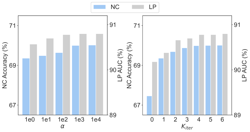
Figure 3: The effect of different hyper-parameters of CTGC on the Cora dataset ($r$=2.6%) under the 3-shot setting.

IV-F Hyper-parameter Sensitivity Analysis (Q6)

In this section, we examine the impact of hyper-parameters on our proposed method across various downstream tasks. The hyper-parameters $\alpha$ adjust the weight of the centroid discrimination loss during the training process. $K_{iter}$ dictates the number of iterations for the alternating optimization of the semantic and structural branches. Fig. 3 shows the node classification and link prediction performance on the Cora dataset.

We select a broad range of values for $\alpha$ to accommodate the gradient variations between the centroid discrimination loss and the cluster loss. As $\alpha$ increases, the model tends to achieve a more uniform distribution of centroids, which supports both node classification and link prediction tasks. The increment of $K_{iter}$ generally enhances model performance and leads to gradual convergence. However, higher values of $K_{iter}$ lead to greater computational demands, necessitating the selection of an appropriate value to balance performance gains with computational complexity.

IV-G Statistics of Condensed Graphs (Q7)

In Table XI, we compare the properties of condensed graphs to those of original graphs. Benefiting from self-supervised learning, the condensed graphs generated by our method not only perform better on downstream tasks but also contain fewer nodes and require significantly less storage. For example, the storage required for the condensed graph of the Reddit dataset is 0.6 MB, which is 726 $\times$ smaller than that required by the original graph. Additionally, these condensed graphs are denser than the original graphs. Given their considerably smaller scale, this increased density enhances message-passing between nodes, benefiting the performance across diverse downstream tasks.

V Related Work

V-A Graph Condensation

Graph condensation [66, 67, 68] focuses on diminishing the computational demands of GNN training through a data-centric approach. It has found widespread application due to its superior capabilities in graph reduction, which includes accelerating inference [69], facilitating continual learning [70], optimizing hyper-parameter/neural architecture search [71], federated learning [11] and backdoor attacks [72].

Research in this area can be grouped into five main categories based on their objectives: effective GC, generalized GC, efficient GC, fair GC, and robust GC. These categories aim to refine the condensation process from different perspectives: Effective GC strategies focus on maximizing the accuracy of GNNs trained on condensed graphs. Such strategies often include sophisticated optimization techniques to improve results, including trajectory matching [14], kernel ridge regression [13], and graph neural tangent kernels [73] to preserve crucial structural and feature data necessary for optimal GNN performance. Notably, SGDC [28] employs self-supervised learning to boost the quality of condensed graphs, but it limits its focus to graph-level data and the graph classification task.

Generalized GC [74] seeks to enhance the performance of various GNN architectures on condensed graphs. It tackles the challenge of minimizing information loss during the condensation process. For instance, SGDD [20] uses Laplacian energy distribution to examine graph structural properties, assessing the spectral difference between condensed and training graphs. GCEM [27] avoids conventional reliance on relay GNNs and instead directly produces the eigenbasis for the condensed graph, eliminating the spectral bias of relay GNNs.

Efficient GC [16] focuses on the speed of creating condensed graphs and their application in time-critical scenarios. These methods streamline the entire GC process, from graph encoding to optimization and generation, drastically reducing the time needed for condensation. CGC [17] consolidates existing optimization techniques into a distribution matching approach and transforms the optimization process into a clustering task that can be efficiently executed without extensive training.

Fair GC addresses the potential disparities in fairness between models trained on condensed and original graphs [75], aiming to prevent the amplification of biases within condensed graphs and ensure fair model performance.

Lastly, Robust GC [76] targets the integrity of the condensation process by filtering out noise from the original graphs, focusing only on vital, causative information for the condensed graph to ensure effective GNN training. This approach helps to prevent the propagation of noise from the original graphs to the GNNs, thereby preserving the accuracy of model predictions.

V-B Graph Self-Supervised Learning

Self-supervised learning (SSL) in graph representation learning [77] has proven to enhance model generalization across different tasks. SSL constructs specific tasks using unlabeled data, allowing models to identify and learn significant patterns in graph data, thereby reducing reliance on labeled data. This approach generally improves model performance in various downstream applications. The essence of SSL lies in designing the surrogate task, with current methods falling into three broad categories: contrastive, generative, and predictive.

Contrastive learning focuses on maximizing the similarity between two jointly sampled positive pairs while minimizing similarity with sampled negative pairs. The scope of these pairs can vary from local [78, 79], contextual [36], to global [78], aligning with node-level, subgraph-level, or graph-level information, respectively. Additionally, contrastive learning approaches involve comparing two graph views, either within the same scale or across different scales, dividing these methods into same-scale contrasting [80] and cross-scale contrasting categories [81]. On the other hand, generative approaches leverage generative models to preserve crucial information from the graph. These methods encode the graph into compact representations [82] and then reconstruct it to retain essential features of the original structure [83] or node attributes [84], focusing on the fidelity of the reconstruction. Finally, predictive methods generate informative labels from the graph data itself to serve as self-supervision. These labels are derived from various graph properties such as node degree [36], node labels [85], or the shortest paths [86], thus creating a direct correlation between the data and the labels.

In the SSL context, our proposed CTGC model employs a contrastive SSL approach by encouraging node embeddings to align closely with their cluster center and neighboring nodes, which falls into the categories of local-local and local-context contrastive tasks.

VI Conclusion

In this paper, we present Contrastive Graph Condensation (CTGC), a novel self-supervised GC approach to efficiently handle diverse downstream tasks. CTGC employs a dual-branch framework to separately extract latent semantic and geometric information. These branches are optimized through a unified self-supervised surrogate task within an alternating optimization framework, facilitating the alignment and mutual enhancement of the two branches. Eventually, the condensed graph is generated using the model inversion technique, which eliminates the dependence on class labels in the GC process and allows for the independent generation of condensed graphs. While CTGC demonstrates promising cross-task generalizability, future research could focus on developing foundation GC methods applicable across various datasets.

References

- [1] X. Gao, W. Zhang, J. Yu, Y. Shao, Q. V. H. Nguyen, B. Cui, and H. Yin, “Accelerating scalable graph neural network inference with node-adaptive propagation,” in 2024 IEEE 40th International Conference on Data Engineering (ICDE). IEEE, 2024, pp. 3042–3055.
- [2] W. Zhang, X. Gao, L. Yang, M. Cao, P. Huang, J. Shan, H. Yin, and B. Cui, “Bim: Improving graph neural networks with balanced influence maximization,” in 2024 IEEE 40th International Conference on Data Engineering (ICDE). IEEE, 2024, pp. 2931–2944.
- [3] X. Gao, W. Zhang, T. Chen, J. Yu, H. Q. V. Nguyen, and H. Yin, “Semantic-aware node synthesis for imbalanced heterogeneous information networks,” in Proceedings of the 32nd ACM International Conference on Information and Knowledge Management, 2023, pp. 545–555.
- [4] Z. Guo, K. Guo, B. Nan, Y. Tian, R. G. Iyer, Y. Ma, O. Wiest, X. Zhang, W. Wang, C. Zhang et al., “Graph-based molecular representation learning,” arXiv preprint arXiv:2207.04869, 2022.
- [5] N. Q. V. Hung, H. H. Viet, N. T. Tam, M. Weidlich, H. Yin, and X. Zhou, “Computing crowd consensus with partial agreement,” IEEE Transactions on Knowledge and Data Engineering, vol. 30, no. 1, pp. 1–14, 2017.
- [6] Q. V. H. Nguyen, C. T. Duong, T. T. Nguyen, M. Weidlich, K. Aberer, H. Yin, and X. Zhou, “Argument discovery via crowdsourcing,” The VLDB Journal, vol. 26, pp. 511–535, 2017.
- [7] W. Jiang, X. Gao, G. Xu, T. Chen, and H. Yin, “Challenging low homophily in social recommendation,” in Proceedings of the ACM on Web Conference 2024, 2024, pp. 3476–3484.
- [8] B. Zheng, K. Zheng, X. Xiao, H. Su, H. Yin, X. Zhou, and G. Li, “Keyword-aware continuous knn query on road networks,” in 2016 IEEE 32Nd international conference on data engineering (ICDE). IEEE, 2016, pp. 871–882.
- [9] W. Zhang, Y. Shen, Z. Lin, Y. Li, X. Li, W. Ouyang, Y. Tao, Z. Yang, and B. Cui, “Pasca: A graph neural architecture search system under the scalable paradigm,” in Proceedings of the ACM Web Conference 2022, 2022, pp. 1817–1828.
- [10] S. Rebuffi, A. Kolesnikov, G. Sperl, and C. H. Lampert, “icarl: Incremental classifier and representation learning,” in 2017 IEEE Conference on Computer Vision and Pattern Recognition, CVPR 2017, Honolulu, HI, USA, July 21-26, 2017, 2017.
- [11] Q. Pan, R. Wu, T. Liu, T. Zhang, Y. Zhu, and W. Wang, “FedGKD: Unleashing the power of collaboration in federated graph neural networks,” arXiv, 2023.
- [12] W. Jin, L. Zhao, S. Zhang, Y. Liu, J. Tang, and N. Shah, “Graph condensation for graph neural networks,” in International Conference on Learning Representations, 2022.
- [13] W. Jin, X. Tang, H. Jiang, Z. Li, D. Zhang, J. Tang, and B. Yin, “Condensing graphs via one-step gradient matching,” in Proceedings of the 28th ACM SIGKDD Conference on Knowledge Discovery and Data Mining, 2022, pp. 720–730.
- [14] X. Zheng, M. Zhang, C. Chen, Q. V. H. Nguyen, X. Zhu, and S. Pan, “Structure-free graph condensation: From large-scale graphs to condensed graph-free data,” in NeurIPS, 2023.
- [15] L. Wang, W. Fan, J. Li, Y. Ma, and Q. Li, “Fast graph condensation with structure-based neural tangent kernel,” WWW, 2024.
- [16] B. Zhao and H. Bilen, “Dataset condensation with distribution matching,” in Proceedings of the IEEE/CVF Winter Conference on Applications of Computer Vision, 2023, pp. 6514–6523.
- [17] X. Gao, T. Chen, W. Zhang, J. Yu, G. Ye, Q. V. H. Nguyen, and H. Yin, “Rethinking and accelerating graph condensation: A training-free approach with class partition,” arXiv preprint arXiv:2405.13707, 2024.
- [18] Y. Liu, R. Qiu, and Z. Huang, “Gcondenser: Benchmarking graph condensation,” arXiv preprint arXiv:2405.14246, 2024.
- [19] E. Dai, W. Jin, H. Liu, and S. Wang, “Towards robust graph neural networks for noisy graphs with sparse labels,” in Proceedings of the Fifteenth ACM International Conference on Web Search and Data Mining, 2022, pp. 181–191.
- [20] B. Yang, K. Wang, Q. Sun, C. Ji, X. Fu, H. Tang, Y. You, and J. Li, “Does graph distillation see like vision dataset counterpart?” in NeurIPS, 2023.
- [21] H. Yin, Q. Wang, K. Zheng, Z. Li, and X. Zhou, “Overcoming data sparsity in group recommendation,” IEEE Transactions on Knowledge and Data Engineering, vol. 34, no. 7, pp. 3447–3460, 2020.
- [22] J. Yu, H. Yin, X. Xia, T. Chen, J. Li, and Z. Huang, “Self-supervised learning for recommender systems: A survey,” IEEE Transactions on Knowledge and Data Engineering, 2023.
- [23] T. Chen, H. Yin, G. Ye, Z. Huang, Y. Wang, and M. Wang, “Try this instead: Personalized and interpretable substitute recommendation,” in Proceedings of the 43rd international ACM SIGIR conference on research and development in information retrieval, 2020, pp. 891–900.
- [24] Y. Wang, X. Yan, C. Hu, Q. Xu, C. Yang, F. Fu, W. Zhang, H. Wang, B. Du, and J. Jiang, “Generative and contrastive paradigms are complementary for graph self-supervised learning,” in 2024 IEEE 40th International Conference on Data Engineering (ICDE), 2024, pp. 3364–3378.
- [25] H. Liu, J. Liu, F. Tang, P. Li, L. Chen, J. Yu, Y. Zhu, M. Gao, Y. Yang, and X. Hou, “Graph contrastive learning for truth inference,” in 2024 IEEE 40th International Conference on Data Engineering (ICDE), 2024, pp. 263–275.
- [26] R. Li, S. Di, L. Chen, and X. Zhou, “Gradgcl: Gradient graph contrastive learning,” in 2024 IEEE 40th International Conference on Data Engineering (ICDE), 2024, pp. 1171–1184.
- [27] Y. Liu, D. Bo, and C. Shi, “Graph distillation with eigenbasis matching,” in Forty-first International Conference on Machine Learning.
- [28] Y. Wang, X. Yan, S. Jin, H. Huang, Q. Xu, Q. Zhang, B. Du, and J. Jiang, “Self-supervised learning for graph dataset condensation,” in Proceedings of the 30th ACM SIGKDD Conference on Knowledge Discovery and Data Mining, 2024, pp. 3289–3298.
- [29] K. Binici, S. Aggarwal, C. Acar, N. T. Pham, K. Leman, G. H. Lee, and T. Mitra, “Condensed sample-guided model inversion for knowledge distillation,” arXiv preprint arXiv:2408.13850, 2024.
- [30] C. Wang, J. Sun, Z. Dong, J. Zhu, Z. Li, R. Li, and R. Zhang, “Data-free knowledge distillation for reusing recommendation models,” in Proceedings of the 17th ACM Conference on Recommender Systems, 2023, pp. 386–395.
- [31] T. N. Kipf and M. Welling, “Semi-supervised classification with graph convolutional networks,” in 5th International Conference on Learning Representations, ICLR 2017, Toulon, France, April 24-26, 2017, Conference Track Proceedings, 2017.
- [32] L. Lin, J. Chen, and H. Wang, “Spectrum guided topology augmentation for graph contrastive learning,” in NeurIPS 2022 Workshop: New Frontiers in Graph Learning, 2022.
- [33] F. R. Chung, Spectral graph theory. American Mathematical Soc., 1997, vol. 92.
- [34] J. R. Lee, S. O. Gharan, and L. Trevisan, “Multiway spectral partitioning and higher-order cheeger inequalities,” Journal of the ACM (JACM), vol. 61, no. 6, pp. 1–30, 2014.
- [35] D. K. Hammond, Y. Gur, and C. R. Johnson, “Graph diffusion distance: A difference measure for weighted graphs based on the graph laplacian exponential kernel,” in 2013 IEEE global conference on signal and information processing. IEEE, 2013, pp. 419–422.
- [36] J. Qiu, Q. Chen, Y. Dong, J. Zhang, H. Yang, M. Ding, K. Wang, and J. Tang, “Gcc: Graph contrastive coding for graph neural network pre-training,” in Proceedings of the 26th ACM SIGKDD international conference on knowledge discovery & data mining, 2020, pp. 1150–1160.
- [37] Y. Zhu, Y. Wang, H. Shi, Z. Zhang, D. Jiao, and S. Tang, “Graphcontrol: Adding conditional control to universal graph pre-trained models for graph domain transfer learning,” in Proceedings of the ACM on Web Conference 2024, 2024, pp. 539–550.
- [38] U. Von Luxburg, “A tutorial on spectral clustering,” Statistics and computing, vol. 17, pp. 395–416, 2007.
- [39] S. Lei and D. Tao, “A comprehensive survey of dataset distillation,” TPAMI, 2024.
- [40] M. Liu, S. Li, X. Chen, and L. Song, “Graph condensation via receptive field distribution matching,” arXiv preprint arXiv:2206.13697, 2022.
- [41] D. Bo, Y. Fang, Y. Liu, and C. Shi, “Graph contrastive learning with stable and scalable spectral encoding,” Advances in Neural Information Processing Systems, vol. 36, 2024.
- [42] Y. Jin, A. Loukas, and J. JaJa, “Graph coarsening with preserved spectral properties,” in International Conference on Artificial Intelligence and Statistics. PMLR, 2020, pp. 4452–4462.
- [43] D. Bo, C. Shi, L. Wang, and R. Liao, “Specformer: Spectral graph neural networks meet transformers,” arXiv preprint arXiv:2303.01028, 2023.
- [44] Y. Zheng, S. Pan, V. Lee, Y. Zheng, and P. S. Yu, “Rethinking and scaling up graph contrastive learning: An extremely efficient approach with group discrimination,” Advances in Neural Information Processing Systems, vol. 35, pp. 10 809–10 820, 2022.
- [45] Y. Liu, K. Liang, J. Xia, S. Zhou, X. Yang, X. Liu, and S. Z. Li, “Dink-net: Neural clustering on large graphs,” in International Conference on Machine Learning. PMLR, 2023, pp. 21 794–21 812.
- [46] M. Douze, A. Guzhva, C. Deng, J. Johnson, G. Szilvasy, P.-E. Mazaré, M. Lomeli, L. Hosseini, and H. Jégou, “The faiss library,” arXiv preprint arXiv:2401.08281, 2024.
- [47] R. Gommers, P. Virtanen, E. Burovski, W. Weckesser, T. E. Oliphant, M. Haberland, D. Cournapeau, T. Reddy, P. Peterson, A. Nelson et al., “scipy/scipy: Scipy 1.9. 0,” Zenodo, 2022.
- [48] W. Hu, M. Fey, M. Zitnik, Y. Dong, H. Ren, B. Liu, M. Catasta, and J. Leskovec, “Open graph benchmark: Datasets for machine learning on graphs,” Advances in neural information processing systems, vol. 33, pp. 22 118–22 133, 2020.
- [49] H. Zeng, H. Zhou, A. Srivastava, R. Kannan, and V. K. Prasanna, “Graphsaint: Graph sampling based inductive learning method,” in 8th International Conference on Learning Representations, ICLR 2020, Addis Ababa, Ethiopia, April 26-30, 2020. OpenReview.net, 2020.
- [50] P. Veličković, W. Fedus, W. L. Hamilton, P. Liò, Y. Bengio, and R. D. Hjelm, “Deep graph infomax,” arXiv preprint arXiv:1809.10341, 2018.
- [51] K. Ding, J. Wang, J. Li, K. Shu, C. Liu, and H. Liu, “Graph prototypical networks for few-shot learning on attributed networks,” in Proceedings of the 29th ACM International Conference on Information & Knowledge Management, 2020, pp. 295–304.
- [52] X. Sun, H. Cheng, J. Li, B. Liu, and J. Guan, “All in one: Multi-task prompting for graph neural networks,” in Proceedings of the 29th ACM SIGKDD Conference on Knowledge Discovery and Data Mining, 2023, pp. 2120–2131.
- [53] M. Welling, “Herding dynamical weights to learn,” in Proceedings of the 26th Annual International Conference on Machine Learning, 2009, pp. 1121–1128.
- [54] F. M. Castro, M. J. Marín-Jiménez, N. Guil, C. Schmid, and K. Alahari, “End-to-end incremental learning,” in Proceedings of the European conference on computer vision (ECCV), 2018.
- [55] O. Sener and S. Savarese, “Active learning for convolutional neural networks: A core-set approach,” arXiv preprint arXiv:1708.00489, 2017.
- [56] R. Z. Farahani and M. Hekmatfar, Facility location: concepts, models, algorithms and case studies. Springer Science & Business Media, 2009.
- [57] A. Loukas, “Graph reduction with spectral and cut guarantees.” J. Mach. Learn. Res., no. 116, 2019.
- [58] Z. Huang, S. Zhang, C. Xi, T. Liu, and M. Zhou, “Scaling up graph neural networks via graph coarsening,” in Proceedings of the 27th ACM SIGKDD conference on knowledge discovery & data mining, 2021, pp. 675–684.
- [59] Z. Xiao, Y. Wang, S. Liu, H. Wang, M. Song, and T. Zheng, “Simple graph condensation,” arXiv preprint arXiv:2403.14951, 2024.
- [60] Z. Liu, C. Zeng, and G. Zheng, “Graph data condensation via self-expressive graph structure reconstruction,” in Proceedings of the 30th ACM SIGKDD Conference on Knowledge Discovery and Data Mining, 2024, pp. 1992–2002.
- [61] W. L. Hamilton, Z. Ying, and J. Leskovec, “Inductive representation learning on large graphs,” in Advances in Neural Information Processing Systems 30: Annual Conference on Neural Information Processing Systems 2017, December 4-9, 2017, Long Beach, CA, USA, 2017, pp. 1024–1034.
- [62] F. Wu, A. Souza, T. Zhang, C. Fifty, T. Yu, and K. Weinberger, “Simplifying graph convolutional networks,” in Proceedings of the 36th International Conference on Machine Learning. PMLR, 2019, pp. 6861–6871.
- [63] A. Bojchevski, J. Gasteiger, B. Perozzi, A. Kapoor, M. Blais, B. Rózemberczki, M. Lukasik, and S. Günnemann, “Scaling graph neural networks with approximate pagerank,” in Proceedings of the 26th ACM SIGKDD International Conference on Knowledge Discovery and Data Mining. New York, NY, USA: ACM, 2020.
- [64] M. Defferrard, X. Bresson, and P. Vandergheynst, “Convolutional neural networks on graphs with fast localized spectral filtering,” in Advances in Neural Information Processing Systems 29: Annual Conference on Neural Information Processing Systems 2016, December 5-10, 2016, Barcelona, Spain, 2016.
- [65] Y. Zhu, W. Xu, J. Zhang, Q. Liu, S. Wu, and L. Wang, “Deep graph structure learning for robust representations: A survey,” arXiv preprint arXiv:2103.03036, vol. 14, pp. 1–1, 2021.
- [66] X. Gao, J. Yu, W. Jiang, T. Chen, W. Zhang, and H. Yin, “Graph condensation: A survey,” arXiv preprint arXiv:2401.11720, 2024.
- [67] M. Hashemi, S. Gong, J. Ni, W. Fan, B. A. Prakash, and W. Jin, “A comprehensive survey on graph reduction: Sparsification, coarsening, and condensation,” arXiv preprint arXiv:2402.03358, 2024.
- [68] H. Xu, L. Zhang, Y. Ma, S. Zhou, Z. Zheng, and B. Jiajun, “A survey on graph condensation,” arXiv preprint arXiv:2402.02000, 2024.
- [69] X. Gao, T. Chen, Y. Zang, W. Zhang, Q. V. H. Nguyen, K. Zheng, and H. Yin, “Graph condensation for inductive node representation learning,” in ICDE, 2024.
- [70] Y. Liu, R. Qiu, and Z. Huang, “CaT: Balanced continual graph learning with graph condensation,” in ICDM, 2023.
- [71] M. Ding, X. Liu, T. Rabbani, T. Ranadive, T.-C. Tuan, and F. Huang, “Faster hyperparameter search for GNNs via calibrated dataset condensation,” arXiv, 2022.
- [72] J. Wu, N. Lu, Z. Dai, W. Fan, S. Liu, Q. Li, and K. Tang, “Backdoor graph condensation,” arXiv preprint arXiv:2407.11025, 2024.
- [73] M. Fey and J. E. Lenssen, “Fast graph representation learning with pytorch geometric,” arXiv preprint arXiv:1903.02428, 2019.
- [74] X. Gao, T. Chen, W. Zhang, Y. Li, X. Sun, and H. Yin, “Graph condensation for open-world graph learning,” in Proceedings of the 30th ACM SIGKDD Conference on Knowledge Discovery and Data Mining, 2024, pp. 851–862.
- [75] Q. Feng, Z. Jiang, R. Li, Y. Wang, N. Zou, J. Bian, and X. Hu, “Fair graph distillation,” in NeurIPS, 2023.
- [76] X. Gao, H. Yin, T. Chen, G. Ye, W. Zhang, and B. Cui, “Robgc: Towards robust graph condensation,” arXiv preprint arXiv:2406.13200, 2024.
- [77] L. Wu, H. Lin, C. Tan, Z. Gao, and S. Z. Li, “Self-supervised learning on graphs: Contrastive, generative, or predictive,” IEEE Transactions on Knowledge and Data Engineering, vol. 35, no. 4, pp. 4216–4235, 2021.
- [78] Y. Zhu, Y. Xu, F. Yu, Q. Liu, S. Wu, and L. Wang, “Deep graph contrastive representation learning,” arXiv preprint arXiv:2006.04131, 2020.
- [79] Y. Liu, X. Gao, T. He, T. Zheng, J. Zhao, and H. Yin, “Reliable node similarity matrix guided contrastive graph clustering,” IEEE Transactions on Knowledge and Data Engineering, 2024.
- [80] V. Verma, T. Luong, K. Kawaguchi, H. Pham, and Q. Le, “Towards domain-agnostic contrastive learning,” in International Conference on Machine Learning. PMLR, 2021, pp. 10 530–10 541.
- [81] W. Hu, B. Liu, J. Gomes, M. Zitnik, P. Liang, V. Pande, and J. Leskovec, “Strategies for pre-training graph neural networks,” arXiv preprint arXiv:1905.12265, 2019.
- [82] Z. Hu, Y. Dong, K. Wang, K.-W. Chang, and Y. Sun, “Gpt-gnn: Generative pre-training of graph neural networks,” in Proceedings of the 26th ACM SIGKDD international conference on knowledge discovery & data mining, 2020, pp. 1857–1867.
- [83] Y. You, T. Chen, Z. Wang, and Y. Shen, “When does self-supervision help graph convolutional networks?” in international conference on machine learning. PMLR, 2020, pp. 10 871–10 880.
- [84] W. Jin, T. Derr, H. Liu, Y. Wang, S. Wang, Z. Liu, and J. Tang, “Self-supervised learning on graphs: Deep insights and new direction,” arXiv preprint arXiv:2006.10141, 2020.
- [85] Q. Li, Z. Han, and X.-M. Wu, “Deeper insights into graph convolutional networks for semi-supervised learning,” in Proceedings of the AAAI Conference on Artificial Intelligence, vol. 32, no. 1, 2018.
- [86] Z. Peng, Y. Dong, M. Luo, X.-M. Wu, and Q. Zheng, “Self-supervised graph representation learning via global context prediction,” arXiv preprint arXiv:2003.01604, 2020.