Abstract

Background: The success of embolisation, a minimally invasive treatment of liver cancer, could be evaluated in the operational room with cone-beam CT by acquiring a dynamic perfusion scan to inspect the contrast agent flow.
Purpose: The reconstruction algorithm must address the issues of low temporal sampling and higher noise levels inherent in cone-beam CT systems, compared to conventional CT.
Methods: Therefore, a model-based perfusion reconstruction based on the time separation technique (TST) was applied. TST uses basis functions to model time attenuation curves. These functions are either analytical or based on prior knowledge, extracted using singular value decomposition of the classical CT perfusion data of animal subjects. To explore how well the prior knowledge can model perfusion dynamics and what the potential limitations are, the dynamic CBCT perfusion scan was simulated from a dynamic CT perfusion scan under different noise levels. The TST method was compared to static reconstruction.
Results: It was demonstrated on this simulated dynamic CBCT perfusion scan that a set consisting of only four bases results in perfusion maps that preserve relevant information, denoises the data, and outperforms static reconstruction under higher noise levels. TST with prior knowledge would not only outperform static reconstruction, but also the TST with analytical bases. Furthermore, it has been shown that only eight CBCT rotations, unlike previously assumed ten, are sufficient to obtain the perfusion maps comparable to the reference CT perfusion maps. This contributes to saving dose and reconstruction time. The real dynamic CBCT perfusion scan, reconstructed under the same conditions as the simulated scan, shows potential for maintaining the accuracy of the perfusion maps. By visual inspection, the embolised region was matching to that in corresponding CT perfusion maps.
Conclusions: CBCT reconstruction of perfusion scan data using the TST method has shown promising potential, outperforming static reconstructions and potentially saving dose by reducing the necessary number of acquisition sweeps. Further analysis of a larger cohort of patient data is needed to draw final conclusions regarding the expected advantages of the time separation technique.

 
The work of this paper is funded by the German Ministry of Education and Research (BMBF) within the Forschungscampus STIMULATE under grant no. 13GW0473A and 13GW0473B.
The authors have no conflicts to disclose.
 

I. Introduction

Dynamic computed tomography perfusion (dCTp) imaging of the liver is an important non-invasive modality to inspect, quantify and visualise haemodynamic changes in the liver, in order to diagnose and characterise liver cancer, to plan and perform the treatment, and to assess the response to the treatment ^{1, 2}. For a minimally invasive treatment, such as embolisation, it would be beneficial to have cone-beam CT (CBCT), and related CBCT perfusion (dCBCTp) acquisition protocols, within the interventional suite, so the patient does not have to be moved outside of the operating room ^{3, 4}. In this way, not only the tumour-feeding vessels could be detected but also it could be inspected whether the blood flow to the desired region was blocked ⁵.

The idea for the dynamic liver perfusion imaging using CBCT came from parenchymal perfusion imaging using CBCT and its inability to be comparable to dCTp imaging ^{6, 7}. In perfusion imaging, a contrast agent is injected intravenously to enhance the visibility of the organ’s internal structures. After the injection, a series of time-resolved CT volume images is acquired. For parenchymal perfusion imaging, only one rotation (sweep) around the patient is performed after the injection. In one sweep, lasting $\sim$$4\text{\,}\mathrm{s}$, 2D projections covering $200\text{\,}\mathrm{\SIUnitSymbolDegree}$ angle are acquired. The volume is then reconstructed using all the 2D projections as if all were acquired at the same time point, disregarding the dynamic nature of perfusion⁸. For dynamic perfusion imaging first, more sweeps need to be acquired ⁶ and second, the reconstruction approach should take into account for the time dependency of every acquired 2D projection. Reconstructing the proposed ten separate sweeps ⁶ over a complete scan duration of $\sim$$52\text{\,}\mathrm{s}$ and determining perfusion in this way would be subject to significant errors ⁹.

A model-based approach can utilise the fact that data from every projection angle are recorded multiple times, i.e., once in every sweep, to mitigate undersampling problems. In case of the dCBCTp perfusion of the brain, the so-called time separation technique (TST) was used to denoise the data and accurately estimate time attenuation profiles of the contrast agent ^{10, 11, 12}. The TST uses an orthogonal basis functions set (BFS) to model the perfusion dynamics, so the reconstruction problem is simplified and the overall computational time is reduced. In this research applicability and potential advantages of TST for liver perfusion imaging with dCBCTp were investigated. The algorithms were tested using animal models, where the dCTp and matching dCBCTp scans of an in vivo swine liver with embolised tissue were acquired ¹³.

II. Methodology

II.A. Data Acquisition

Three corresponding dCTp and dCBCTp scans of three different pig livers were acquired with a SOMATOM Force CT and an ARTIS pheno robotic C-arm system (Siemens Healthineers AG, Forchheim, Germany). The three animals were labelled with numbers from 1 to 3. The study was conducted in accordance with the European Directive 2010/63/EU and with the German law for animal protection (TierSchG). All experiments were approved by the local animal ethics committee (Lower Saxony State Office for Consumer Protection and Food Safety, LAVES 18/2809).

The three dCBCTp scans were acquired using the same acquisition protocols (see Table 1). The subsegment artery of the right hepatic artery was embolised with Onyx(R) (Medtronic, Meerbusch, Germany). The contrast material Imeron 300 was injected into the right hepatic artery. The C-arm performs 10 rotations in a bidirectional manner, pausing between consecutive rotations. In this way, five forward and five backward sweeps are acquired. The first two sweeps are mask sweeps, one for the forward and one for the backward rotation as shown in Fig. 1. Each sweep comprises 248 views. There is an inconsistency between the angles at which the corresponding views with index $i$ in forward and index $(248-i)$ in backward sweep are acquired. The time intervals between two consecutive views, i.e. frame time, differ within the sweep due to the accelerating rotation of the C-arm at the beginning of the scan and decelerating towards the end of the scan. The duration of all dCBCTp scans, including all 10 rotations, is $\sim$$52\text{\,}\mathrm{s}$. The rotation time lies around $3.9\text{\,}\mathrm{s}$ with the pause time between two rotations of $\sim$$1.4\text{\,}\mathrm{s}$.

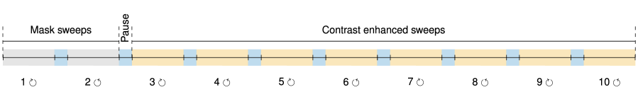
Figure 1: Schema of dynamic CBCT perfusion scan with ten sweep protocol.

The scanning durations of the dCTp scan for animals 1, 2, and 3 were $65.997\text{\,}\mathrm{s}$, $56.997\text{\,}\mathrm{s}$ and $41.998\text{\,}\mathrm{s}$, respectively. The tube peak voltage for the dCTp scans was set to $90\text{\,}\mathrm{k}\mathrm{v}$. The matching dCBCTp and dCTp scans have the same contrast agent injection protocols as documented in Table 2. The animals were in general anesthesia with muscle relaxation to avoid any muscle movements such as breathing.

Table 1: The acquisition protocol for dynamic CBCT perfusion scan.

Duration	$\sim$$52\text{\,}\mathrm{s}$
Number of 3D rotations	10
Number of views per rotation	248
Angle covered	$200\text{\,}\mathrm{\SIUnitSymbolDegree}$
Angle step	$0.8\text{\,}\mathrm{\SIUnitSymbolDegree}$
Detector size (no. of pixels)	624 x 464
Pixel spacing	0.16 x 0.16 ${\mathrm{mm}}^{2}$
Tube peak voltage	$90\text{\,}\mathrm{kV}$

Table 2: Contrast agent injection protocols for three scans.

	Contrast agent
Scan	Dose	Flow rate	Flow duration	Volume
	[ml]	[ml/s]	[s]	[ml]
1	$14.0$	$3.0$	$7.0$	$20.0$
2	$10.43$	$2.8$	$5.07$	$14.9$
3	$10.43$	$2.9$	$5.1$	$14.9$

II.B. CBCT scan simulation

As the different positioning of the animal in CT and in the corresponding CBCT makes it difficult to compare both volumes voxel-wise, the dCBCTp scan was simulated by reprojecting the dCTp scan, referred to as rdCBCTp. Due to data limitation (see Sec. II.D.2.) only the shortest dCTp scan was reprojected. To maintain a realistic rotation velocity of the C-arm, the rdCBCTp scan consists of eight contrast-enhanced sweeps. The time-resolved volumes are interpolated using Akima splines ¹⁴, and resampled at time points defined by the frame times of the original corresponding dCBCTp scan during eight sweeps. These were estimated from the DICOM header Frame Time Vector. The forward projector algorithm of the CT Library ¹⁵ was used to simulate dCBCTp projection data from the dCTp volumes, where the projection matrix of the forward sweep of the real dCBCTp scan was used to model the geometry. To avoid the need for 2D-2D registration to compensate for angle inconsistency of forward and backward sweeps, the order of the forward projection matrix was reversed to estimate the backward sweep geometry. Although the breathing was suppressed, some motion is still present in the intestines.

The voxel size for reconstruction is the same as the voxel size of the matching CT scan, ($0.7305\text{\,}\mathrm{m}\mathrm{m}$, $0.7305\text{\,}\mathrm{m}\mathrm{m}$, $1.5\text{\,}\mathrm{m}\mathrm{m}$). The voxel count in one volume is $512\times 512\times 175$.

II.B.1. Noise Addition

Considering that the CBCT scans suffer from higher noise levels than CT, two different levels of Poisson noise, higher noise of $2.1\text{\times}{10}^{5}$ photons per ${\mathrm{mm}}^{2}$ and moderate noise of $6\text{\times}{10}^{5}$ photons per ${\mathrm{mm}}^{2}$ at the detector ^{16, 17}, were added to reprojected dCBCTp scan.

II.C. Reconstruction

The reconstruction from the dCTp scan is a 4D reconstruction task because the contrast enhancement varies dynamically during the acquisition of the volume time series. Each voxel in the volume is defined by the four coordinates, $(x,y,z,t)$, where $z$ denotes the slice, $x,y$ the positions of the voxel in the slice, and $t\in\mathcal{I}$ represents a time point during the scan duration $\mathcal{I}$. The time attenuation curve (TAC) describes the contrast agent dynamics in each voxel at all sampling time points $t$. TACs are extracted from the reconstructed volumes. Therefore, the reconstruction problem is a time-dependent CT problem.

$$\mathbf{A}\mathbf{x}(t)=\mathbf{p}(t)\quad t\in\mathcal{I}$$ (1)

where $\mathbf{A}$ is the system matrix that maps volume $\mathbf{x}$ at time point $t$ onto the projection space $\mathbf{p}$.

In a dCBCTp scan at a single time point $t\in[0,T_{s}]$, where $T_{s}=4s$ is the duration of one sweep, a 2D projection for one source-detector position, i.e., angle $\varphi_{i},i\in\{1,..,\Phi\}$, is acquired. In ten-sweep acquisition protocol, only 10 projections for the same $\varphi_{i}$ are acquired over the scan duration $T=52s$. This makes the reconstruction problem Eq. 1 in the domain of dCBCTp scan reconstruction underdetermined. The time interval for the same $\varphi_{i}$ between every two sweeps, due to a bidirectional rotation of the C-arm and pause time between sweeps is not constant.

In the straightforward reconstruction approach ¹², each sweep is reconstructed separately under the assumption that all the projections in one sweep have been acquired at the same time point, and thus the dynamic change of contrast agent flow through the organ is not properly represented. This limits the quantifiability of the perfusion maps.

The TST ^{11, 12} relies on the idea of model-based reconstruction (MBR). Both voxels’ dynamics $\textbf{x}(t)$ and projections $\textbf{p}(t)$ are represented as the linear combination of the same orthonormal basis functions set (Eq. 2).

$$\mathcal{B}=\{\Psi_{1},\ldots,\Psi_{N}\},\quad N\rightarrow\infty$$ (2)

Furthermore, the TST assumes that with a very suitable orthonormal bases (see Sec. II.D.2.), only the first $\hat{N}\leq 5$ elements would be sufficient to model perfusion.

Each voxel $x_{v}(t)$ is represented as

$$x_{v}(t)=\sum_{i=1}^{\infty}{w_{v,i}}\Psi_{i}(t)\approx\sum_{i=1}^{\hat{N}}{w_{v,i}}\Psi_{i}(t)$$ (3)

and each projection pixel $p_{n}$

$$p_{n}(t)=\sum_{j=1}^{\infty}{c_{n,j}}\Psi_{j}(t)\approx\sum_{j=1}^{\hat{N}}{c_{n,j}}\Psi_{j}(t),$$ (4)

where $v$ codes $(x,y,z)$ coordinates in the volume and $n$ codes $(u,v,\varphi)$ coordinates in the projection images. Using this notation, the reconstruction problem in Eq. 1 takes the form

$$\bm{A}\sum_{i=1}^{\hat{N}}\bm{w}_{i}\Psi_{i}(t)=\sum_{j=1}^{\hat{N}}\bm{c}_{j}\Psi_{j}(t)\quad t\in\mathcal{I}.$$ (5)

As the basis functions form a set of orthogonal vectors, the scalar product of two differing basis functions is zero. By performing the scalar product on both sides of Eq. 5

$$\bm{A}\sum_{i=1}^{\hat{N}}\bm{w}_{i}\langle\Psi_{i}(t),\Psi_{l}(t)\rangle=\sum_{j=1}^{\hat{N}}\bm{c}_{j}\langle\Psi_{j}(t),\Psi_{l}(t)\rangle\quad t\in\mathcal{I},$$ (6)

the reconstruction problem Eq. 1 becomes $\hat{N}$ separate CT problems

$$\bm{Aw}_{i}=\bm{c}_{i}\quad i\in\hat{N},$$ (7)

which simplifies the reconstruction task in such a way that the number of reconstructions that need to be performed equals the number of bases $\hat{N}$ used to model the time dynamics.

Now, $\bm{c}$ from Eq. 4 are determined by calculating the scalar product

$$\langle\bm{p(t)},\Psi(t)\rangle.$$ (8)

The calculation of scalar product is problematic since it assumes that the bases are already sampled at the time points at which the projections are acquired. To carry out the integration for the scalar product estimation, the interpolation of the projections would be acquired, which would lead to significant errors. To circumvent this problem, an optimisation approach was applied as follows:

$$\min_{\{c\}}\left\lVert\Psi(t)\cdot\bm{c}-\bm{p}(t)\right\rVert^{2}=:\bm{c}^{\prime}.$$ (9)

Instead of determining the coefficients $\bm{c}$ from the scalar products, they are defined as the parameters that best approximate the function $\bm{p}$. It should be noted that this fitting method leads to the following approximation

$$\bm{p}(t)=\sum_{i=1}^{\infty}\bm{c}_{i}\Psi_{i}(t)\approx\sum_{i=1}^{\hat{N}}\bm{c}^{\prime}_{i}\Psi_{i}(t).$$ (10)

The prerequisite step is to resample the basis functions at time points specific to each pixel $p_{(x,y,\varphi)}$. Subsequently, these fitted projections are reconstructed and the coefficients $\bm{w}_{i},i\in\{1,..,\hat{N}\}$ are obtained. From these reconstructed coefficients, the time series of volumes for a given sampling can be computed.

The choice of a proper reconstruction algorithm is only limited by Eq. 7. Here, all the reconstructions are computed using a Krylov method based iterative reconstruction to reduce the computation time¹⁸.

II.D. Basis Function Sets

The bases have to be suitable for modelling the contrast agent flow, i.e., to approximate the contrast agent flow with as few as $\hat{N}$ bases. Thus, two different BFSs are used, an analytical BFS and a prior knowledge BFS.

II.D.1. Analytical Set

A set of trigonometric functions (see Eq.11) was successfully used to model brain perfusion ¹². Furthermore, the same bases set was also used to model liver perfusion using a real dCBCTp scan ¹³. The first basis is a constant necessary to model static behaviour of the anatomical background.

$$\begin{split}\Psi_{0}=1,\Psi_{1}=\sin(\frac{2\pi t}{T}),\Psi_{2}=\cos(\frac{2\pi t}{T}),\Psi_{3}=\sin(\frac{4\pi t}{T}),\Psi_{4}=\cos(\frac{4\pi t}{T})\end{split}$$ (11)

II.D.2. Prior Knowledge Set

The prior knowledge BFS extracted from the CT perfusion time-resolved volumes should optimally model the dynamics of liver perfusion¹⁹. Here, the prior knowledge (PK) BFS was extracted from CT time series of only two animals; see Fig. 2. This BFS was tested against the third dCBCTp and rdCBCTp scan.

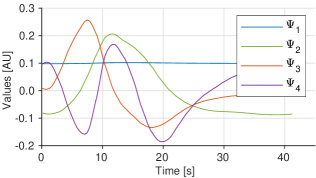
Figure 2: Prior knowledge basis functions set extracted from two animals.

The organ was manually segmented in all slices of CT volumes. All the abdominal organs (intestines, gallbladder, stomach), bones (spine and ribs), surrounding vessels (e.g., gastric artery) and reconstruction artefacts caused by embolisation material were excluded. Orthonormal basis functions were extracted from these volumes using SVD ²⁰. The number of the singular vectors forming the set is determined by the elbow method²¹, and all remaining vectors were considered as noise and omitted. In this work the number of selected basis functions was $\hat{N}=4$.

The SVD is applied only within the duration of the shortest scan — $\sim$$42\text{\,}\mathrm{s}$, meaning it is covering all eight sweeps in rdCBCTp scan. Applying SVD over longer scan duration, would assume that the volumes of the shortest scan wouldn’t be able to cover the whole interval and the cross-validation would not be possible. For extraction of PK, the two scans were aligned in time with respect to the peak of the arterial input function(AIF). The aligning is performed by shifting one of the scans in time. The AIF was selected based on its peak value and time point at which this peak occurred. Fig. 3 shows how the time alignment is performed w.r.t. the duration of the scans via the AIF.

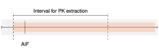
Figure 3: Time alignment of two CT perfusion scans (grey and orange) with respect to the AIF for extraction of prior knowledge.

II.D.3. Time Shifting of Bases

The PK and the projections are time dependent and to model the contrast agent flow through the organ correctly, the PK might need to be shifted in time. The shift is determined after the time alignment of CBCT scan and bases interval. The time alignment is performed in the same manner as the alignment of the CT scans for the extraction of the prior knowledge. Two types of time shifting are to be differentiated but not mutually exclusive. The first type of the shifting occurs when the bases cannot support the whole CBCT scan interval. Then, all the values of the pixel $p_{(x,y,\varphi)}$ that were acquired outside the supported interval, at the beginning or at the end of the scan, will be excluded from the fit (see Fig. 4).

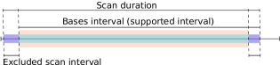
Figure 4: Bases time shifting. Exclusion of projections (purple) from the CBCT scan which are not supported by the bases.

The second shift occurs when the bases interval has to be cropped. Then both, offset at the beginning and the offset at the end of the bases interval could be needed (see Fig. 5).

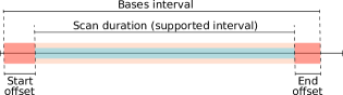
Figure 5: Bases offsetting (red) when the covering interval is longer than the duration of the CBCT scan.

For the data used in this work, only the first type of basis shifting was needed. For the real dCBCTp scan the projections of the first two mask sweeps were outside the supported interval, meaning that the fitting started at the beginning of the third sweep. The AIF of the rdCBCTp reaches its peak value $1.5\text{\,}\mathrm{s}$ after the AIF based on which the CT scans for the PK were aligned so all the projections from the first $1.5\text{\,}\mathrm{s}$ were excluded from the fitting.

II.E. Calculation of Perfusion Maps

The final step in perfusion imaging is the calculation of the perfusion maps. Perfusion maps are the visualisation of the perfusion parameters. The first volume is considered a mask sweep and is subtracted from all the following volumes in time series so that the perfusion parameters can be calculated ²². With the TST, the value of each voxel in time point over the scanning interval is estimated using reconstructed coefficients and the BFS. The first estimated value is subtracted from the rest, so that the time attenuation curve represents only the time dynamics of the voxel.

Since a small amount of contrast agent was injected into the right hepatic artery at a high rate, no contrast agent is expected in the portal vein during the acquisition time. Therefore, only four perfusion parameters are calculated in the arterial phase, blood flow (BF), blood volume (BV), mean transit time (MTT) and time to peak (TTP). Previously, it was shown that the embolised regions are better distinguishable in perfusion maps calculated using the deconvolution method in comparison to the maximum slope approach. Also, the MTT can be miscalculated with the maximum slope approach even with the high injection rate of contrast agent ^{23, 24}. Thus, the perfusion parameters are calculated here using a deconvolution algorithm²⁵.

The perfusion parameters are calculated voxel-wise. The TAC of each voxel $v$, $tac_{v}(t)$ is represented as a convolution of arterial input function (AIF) $aif(t)$ and convolution kernel $k_{v}\mathrm{(t)}$

$$\mathrm{tac_{i}(t)}=\mathrm{aif(t)}*k_{i}\mathrm{(t)}.$$ (12)

This problem can be represented algebraically

$$\mathbf{Ak}=\mathbf{c}$$ (13)

where $\mathbf{A}$ is the Toeplitz matrix constructed from discretised AIF. Now, $\mathbf{k}$ is found by solving

$$\mathbf{k}=\mathbf{A}^{-1}\mathbf{c}.$$ (14)

SVD is applied on $\mathbf{A}$, then all singular values larger than the Tikhonov regulariser $\lambda_{rel}=0.3*\sigma_{max}$ are inverted, $\sigma=1/\sigma$, and all smaller than $\lambda_{rel}$ set to $\sigma=0$. This way the new matrix $\mathbf{A}^{\prime}$ is formed and, $\mathbf{A}^{-1}$ is replaced by it, so that

$$\mathbf{k}^{\prime}=\mathbf{A}^{\prime}\mathbf{c}$$ (15)

can be estimated ²⁵. Once $\mathbf{k}^{\prime}$ is estimated, the perfusion parameters for each voxel $v$ with TAC sampled in $n=100$ points are calculated as follows

$$\begin{split}BF_{v}=max\{k_{v,i},i\in\{1..n\}\},\quad BV_{v}={\sum_{i=1}^{n}k_{v}},\quad MTT_{v}=\frac{BV_{v}}{BF_{v}}.\end{split}$$ (16)

The TTP is not dependent on the convolution kernel, but only on the TAC and it equals the time point at which the TAC reaches its peak enhancement.

For the visualisation of perfusion maps, the ASIST ²⁶ colourmap is used. With this colourmap, the hypo-perfused — in this case embolised (dark blue), region is easily distinguishable from the healthy perfused tissue. For all perfusion maps, the lower values are represented with cold colours and vice versa for higher values. A Gaussian blur with $\sigma=$3.0\text{\,}\mathrm{p}\mathrm{x}$$ is applied slice-wise to the organ in the perfusion map to ensure noise reduction and for features to be better distinguishable.

II.E.1. Selection of Arterial Input Function

The wrong selection of the AIF can result in a miscalculation of the perfusion parameters. The AIF was localised in a single voxel¹². First, the region of interest (ROI) in a vessel in which the contrast agent was injected was selected. Here, the ROI was selected in the right hepatic artery. From this region a single voxel is selected to be the AIF. The AIF should be selected in the same region for CT and rCBCT²⁷, and when possible in the real CBCT volume as well. Selecting AIFs in different vessels would not only affect the calculation of the perfusion parameter values, but also the overall quality of the perfusion maps. The AIF with the highest peak reached in the earliest time point was selected as the single-point AIF.

II.F. Evaluation of Perfusion Maps

II.F.1. Simulated Dynamic CBCT Perfusion Scan

Simulation of the dCBCTp scan enables voxel-wise comparison of the perfusion maps by calculating the Pearson correlation for every slice. This is possible since the organ is not displaced compared to the dCTp scan. As a consequence, it has suffered from organ truncation not only in the $z$-axis but also in the $xy$-plane. In addition, the motion of the intestines was captured, which can result in streak artefacts. Thus, to analyse only reconstructed voxels that are not severely affected by these occurrences, an additional mask excluding these regions was used for calculation of Pearson correlation coefficients.

II.F.2. Real Dynamic CBCT Perfusion Scan

The position of the animal during the dCTp scan was not the same as during the real dCBCTp scan. To fit it into the field of view of the C-arm CT, the animal was shifted and tilted. Thus, only a qualitative assessment was performed through visual inspection. To find the corresponding slices, features in the slice, such as position of the gallbladder, stomach, ribs and spine were located and compared.

III. Results

III.A. Simulated Dynamic CBCT Perfusion Scan

In Figures 6, 7 and 8, the AIFs are shown for all three noise level scenarios in rCBCT, no noise, moderate noise and high noise level, after the additional Gaussian smoothing was added to CT and CBCT volumes for calculation of perfusion parameters. The TAC for AIF in CT is obtained for the denoted voxels from all time series volumes, in the static reconstruction from reconstructed volumes for every sweep, and in MBR with the TST - from time-resolved volumes. The noise affects the AIF reached peak values but not the overall relation between them compared to the CT AIF. For all rCBCT AIFs, the peak value is lower compared to the reference CT AIF except for the TST with prior knowledge with high noise. The AIF peak of TST with analytical bases is the only one close in time to the reference CT AIF occurring $0.43\text{\,}\mathrm{s}$ later. The same is observable in all three noise levels. Modelling the AIF with analytical basis functions (rCBCT TST-Analytical) can result in an additional peak so that it resembles the peak due to reperfusion or reinjection of contrast agent material. The occurrence of the AIF peak for static reconstruction almost $5\text{\,}\mathrm{s}$ earlier is due to an assumption that all the views within one sweep are considered to be acquired within the same time point. The AIF similarity in shape is observable in all noise scenarios for the AIF modelled by the prior knowledge(rCBCT TST-PK).

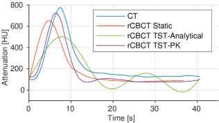
Figure 6: Arterial input functions in reprojected dCBCTp scan with no noise added.

Figure 7: Arterial input functions in reprojected dCBCTp scan with moderate noise level.

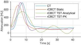
Figure 8: Arterial input functions in reprojected dCBCTp scan with high noise level.

The Pearson correlation coefficients between the CT perfusion maps and rCBCT perfusion maps using AIFs from the Figures 6, 7 and 8, for static reconstruction (”Static”) and MBR by the means of TST using analytical (”Analytical”) and prior knowledge basis functions (”Prior”) are given in Table 3. The regions in slices with reconstruction artefacts were not taken into account. For the BF and MTT, the TST with prior knowledge bases outperforms static reconstruction for all three noise scenarios. As noise levels rise, the correlation values for static reconstruction are decrease. Even though the same behaviour is expected, and it is, for all three CBCT reconstructions, it is the most pronounced for the static reconstruction. For the MTT, the Pearson correlation is below $0.5$ for static reconstruction and for TST with analytical bases, unlike $0.7118$ for TST with prior knowledge for high noise. With the TST the change in correlation between different noise levels is smaller than in case of the static reconstruction, with BF remaining the most stable with prior knowledge.The change in AIF values and shape did not indicate these occurrences, since the shape of the CBCT AIFs for moderate and high noise is more similar to CT AIF, see Figures 7 and  8. For BV, the TST with analytical bases is the best and remains this way independently of the noise levels. However, the TST, neither with analytical nor prior knowledge bases, manages to outperform the static reconstruction for TTP, except for the high noise, for the insignificant difference of $0.0009$.

Table 3: Pearson correlation coefficients for rCBCT perfusion maps compared to CT perfusion maps calculated. The highest values are highlighted in bold.

	No noise			Moderate noise			High noise
	Static	TST		Static	TST		Static	TST
		Analytical	Prior		Analytical	Prior		Analytical	Prior
BF	0.9298	0.9112	0.9371	0.9135	0.8902	0.9259	0.8778	0.8597	0.9008
BV	0.8710	0.8930	0.8475	0.8153	0.8451	0.8106	0.7379	0.7792	0.7576
MTT	0.7385	0.7051	0.8220	0.6341	0.5701	0.7778	0.4947	0.4225	0.7118
TTP	0.7735	0.7575	0.7620	0.7145	0.7002	0.7065	0.6356	0.6281	0.6365

The perfusion maps, BF, BV, MTT and TTP, for the slice at the middle of the liver are shown in Fig. 10 for the scenario of moderate noise level. In the first column are the CT perfusion maps, then perfusion maps calculated for simulated dCBCTp scan in order as follows: static reconstruction (”Static”), TST using analytical BFS (”TST Analytical”) and TST using prior knowledge consisting of four bases (”TST Prior”). The hypo-perfused region, i.e., embolised region, is easily distinguishable in all perfusion maps. The healthy tissue, i.e., well perfused regions, are clearly visible as well. The misestimation of perfusion values due to streak artefacts are visible in the upper part of the organ for all four parameters in the rCBCT perfusion maps. For the BF, this is the most pronounced for TST with prior knowledge bases. In static reconstruction and in TST with prior knowledge bases, the underestimation in comparison to CT can be observed, particularly around the vessel structures. This region is pointed by white arrow in 10. Nevertheless, the BV of TST with prior knowledge is the most similar to CT. For the MTT, the misestimation due to the mentioned reconstruction artefacts is observable in static reconstruction and for TST with prior knowledge bases. This region for the MTT in static reconstruction is indicated by a yellow arrow. For all four parameters, the most similar to CT perfusion maps are the ones depicted in the fourth column of the TST with prior knowledge. Under moderate noise, the TST was not yet able to outperform the static reconstruction for the TTP. This can be especially visible for the TTP with TST with prior knowledge. With increasing noise, the TST with prior knowledge appears to be more comparable to CT perfusion maps (see Table 3). The noise was reconstructed and is visible in perfusion maps, see second and third column, unlike for the TST with prior knowledge. Also, some overestimation is visible in static reconstruction, particularly for BV.

III.B. Real Dynamic CBCT Perfusion Scan

In Fig. 9 the AIFs of real dCBCTp scan of the same animal for which the CT scan was reprojected - in this work labelled 3, are shown in order as follows: CT, static reconstruction (”CBCT Static”), TST using analytical bases (”CBCT TST-Analytical”) and TST using prior knowledge bases (”CBCT TST-PK”). All of the AIFs reach their peak at different time points, with the AIF modelled with TST using prior knowledge having the highest peak value. Note that due to different CT modalities, the values of perfusion parameters cannot be compared. The AIF for the static reconstruction is shifted the most, which is expected considering the time considerations for the acquired projections. The analytical bases do have the peak closest in time to the CT peak, but lower. The same was noted for the reprojected CBCT scan. The AIF with TST with prior knowledge is the closest to the CT AIF in peak value.

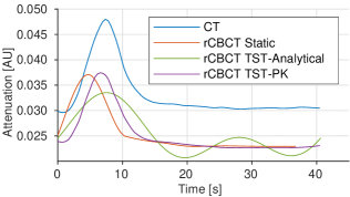
Figure 9: Arterial input functions in real dCBCTp scans .

The perfusion maps for the dCBCTp scan of animal 3 is shown in Fig. 11. The hypo-perfused region is well distinguishable in static and TST with analytical bases. However, for the prior knowledge, some overestimation can be noticed in some regions, which also makes the hypo-perfused region less pronounced - pointed by the yellow arrow. What additionally reduces the quality of perfusion maps are the artefacts, which result in streaks of overperfused regions that are not comparable to the CT scan. However, the MTT with analytical bases is the least comparable to CT perfusion maps. This is particularly visible in the left part of the organ. The BV of TST with analytical bases is showing some underestimation in the upper regions, but with the prior knowledge these overestimations still result in a perfusion map in general more similar to CT. For the MTT, the TST with prior knowledge is overall the most similar. However, the hypo-perfused region is still misinterpreted in terms of TTP - pointed by the white arrow.

Figure 10: Perfusion maps BF, BV, MTT and TTP for dCTp and reprojected dCBCTp scan (static reconstruction, model-based reconstruction with analytical and prior knowledge bases) with moderate noise added. The white arrow is pointing to underestimate BV in prior knowledge and the yellow arrow is pointing to misestimated region due to reconstruction artefacts in MTT for static reconstruction.

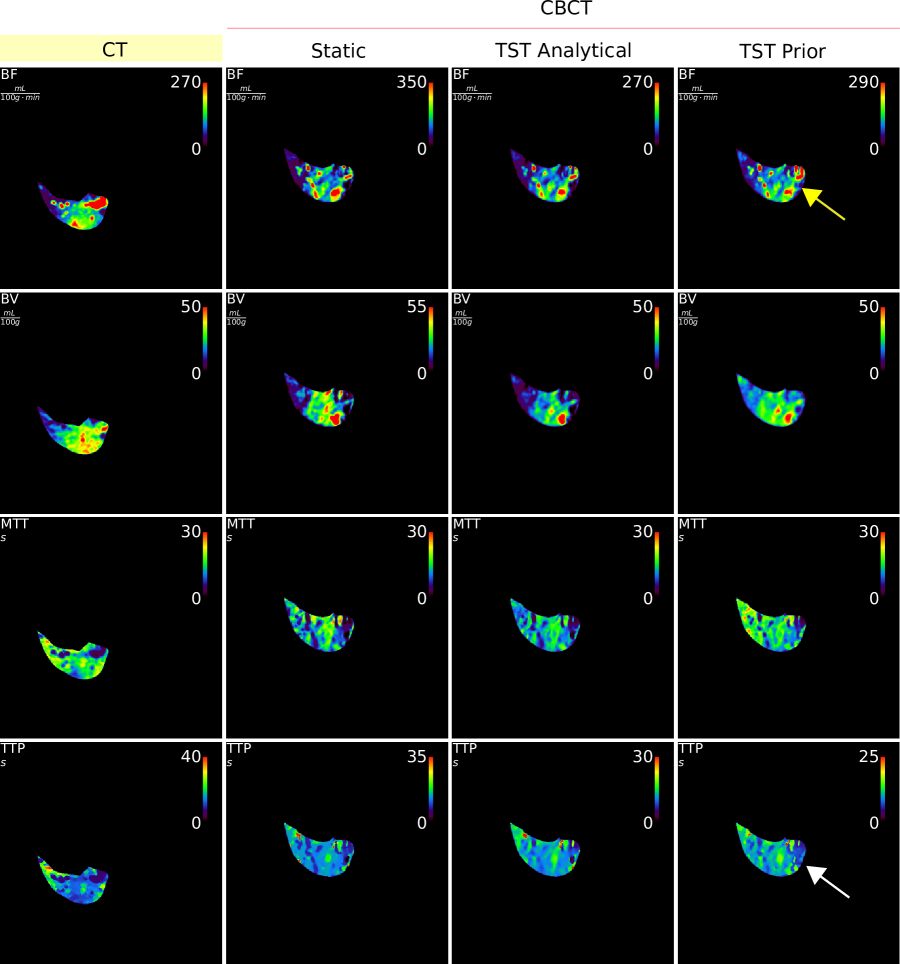
Figure 11: Perfusion maps BF, BV, MTT and TTP calculated using deconvolution method for dCTp and real (i.e. acquired with CBCT) dCBCTp scan (static reconstruction, model-based reconstruction with analytical and prior knowledge bases). The yellow arrow is pointing to overestimated hypo-perfused region in BF for prior knowledge. The white arrow is pointing to misestimated TTP for prior knowledge.

IV. Discussion

In this work, it was shown that the dynamic perfusion CBCT scan of eight sweeps is sufficient for dynamic liver perfusion imaging, which can be beneficial for minimally invasive treatments of liver cancers. Independently of the BFS used, the model-based perfusion reconstruction by the means of TST has provided the perfusion maps in which there is a clear distinction of hypo-perfused region, i.e., the embolised region. This scenario first leads to a shorter scan time and saving radiation dose compared to the proposed scanning protocol⁶ for dynamic CBCT perfusion, and second, it saves computation time due to the lower number of reconstructions that need to be performed. Here, only four bases are enough to describe the dynamic behaviour of the liver. In addition, these bases were only extracted from the CT time-series volumes of two different animals (see Fig. 2), with a slightly different contrast agent injection protocol, and were used to model the dynamics of the third animal. The results show that the TST not only provides the perfusion maps quickly to the radiologist, but also makes the perfusion maps more accurate by compensating for the low temporal sampling. The TST with analytical or prior knowledge bases can outperform static reconstruction, especially for higher noise levels (see Table 3). The AIF was always best modeled by the TST with prior knowledge and the TST with prior knowledge resulted in perfusion maps more similar to CT perfusion maps (see Fig. 10).

The TST with prior knowledge is influenced by many factors that cannot be easily addressed. Here, only two CT scans were available for prior knowledge extraction, and they could not be averaged enough with SVD to try to avoid the necessity of time alignment of CT scans. The time alignment is performed on the basis of the AIF peak position, which is affected by the anatomy of the scanned subjects, the contrast agent injection protocol, and the actual localisation AIF. Next, the scalar product should be calculated, but then insufficient data is available for use to model the dynamics and the interpolation performed based on the very small number of points. Also, depending on the bases shift, either the PK will get violated through the reorthogonalisation or, the CBCT data will be lost due to exclusion of the projections for which the PK is not provided. However, with all these demerits, the TST still managed to model the perfusion correctly under high noise.

CT scans cannot be considered completely noise-free. When the SVD is applied to extract the PK, there is a possibility that some of the noise remains present in singular vectors forming the BFS. For the extraction of the bases, the TACs of CT time-series are interpolated using Akima splines, which can result in error, since with the cubic splines the value between two points can be overestimated.

Although prior knowledge extracted from only two animals was sufficient to reconstruct the dCBCTp scan, it is not clear if the same would be possible for any dCBCTp scan, especially with a different contrast agent injection protocol. Next, the AIF with the BFS formed with more than four bases, namely seven, would have a higher amplitude ¹⁹. However, using more bases causes instabilities in fitting, and inability to produce meaningful perfusion maps ^{11, 19}. Here, already four bases were used to model seven points. Therefore, the number of bases should be kept as low as possible.

The AIF was selected at one single point in static reconstructions, and this makes it susceptible to higher noise. Also, without the 3D registration of the real CBCT and CT volumes, the selection of the AIF in both is only based on the anatomy knowledge. Thus, the AIF could be calculated by weighted averaging of all the voxels from the selected ROI. Without the static reconstruction, the AIF should be selected in one of the reconstructed TST coefficients. For doing so, one should know which of the bases contains the most information about the vessels’ dynamics, and then select the appropriate reconstructed coefficient to select the AIF. This imposes problems for the automation of the AIF selection within the TST approach. Just by selecting a slightly different AIF location or, mistakenly, a completely different vessel in CBCT compared to CT, might result in a completely wrong estimation of the perfusion maps ²⁷. However, it is valuable to note that the actual values of perfusion parameters do not differ much between the comparing perfusion maps and that not for all perfusion parameters. Using the deconvolution method for the estimation of perfusion parameters, the chances of misestimation are lower. With the maximum slope, the values and accuracy would primarily depend on the maximum slope of every TAC, which in the case of secondary peaks, such as for the analytical bases, and not only for the AIF, would contribute to the poor assessment of the perfusion parameters. Alternatively, gamma-variate functions could be fitted to the AIF ²⁸ and to all the TACs, to smooth them out and leave out noise. Not only should the large number of TACs be fitted, but also for each one, the fitting parameters should be adjusted. This is particularly difficult because of the noise that results in multiple peaks in the TAC. At first glance, the idea of fitting gamma variate to also hypo-perfused area might seem good, but these regions are also affected by noise, and even though the peaks in such fitted TACs would be expected to be very low, they could still be wrong in the time domain and falsely represent perfusion.

The contrast agent flow is highly dependent on the anatomy of the subject being scanned. This means that even for exactly the same contrast agent injection protocol, the bases might need to be shifted in time. In this work, this was simulated in such a way that the rdCBCTp had to be shifted in time. The quality of the perfusion maps did not suffer from it even though all the projections acquired in the first $1.5\text{\,}\mathrm{s}$ were excluded, and for these views only seven points could then be used for modelling. Within the real CBCT scan, it was sufficient to simply exclude the mask sweeps. However, by excluding mask sweeps, the baseline needed for the subtraction of static anatomical structures is lost, so the values presented in the perfusion maps are not true to nature. Considering the outflow of the contrast agent and little to no presence in rest of the sweeps, instead of the last two sweeps, two mask sweeps at the beginning could be acquired, without acquiring more than eight sweeps. The time shift could already be estimated in the projection domain by fitting the bases to regions consisting of mostly vessels and selecting the shift with lowest fitting error, which would be very time-consuming. Alternatively, this could be done if the position of the AIF could be assumed in projection domain, since the vessels are visible in contrast-enhanced projections.

The TST is not robust to motion and the motion correction step within it could only be performed in projection domain before the fitting of the bases functions. For shallow breathing ²⁹, the displacement vector could be formed based on the diaphragm position ³⁰. Otherwise, the time-resolved volumes would need to be calculated and registered. The number of points used for TAC sampling for perfusion parameter calculation determines the number of volumes for registration. Furthermore, the rigid registration is not sufficient to compensate for the patient motion, breathing motion, and as a consequence of the breathing, the motion inside the liver. Although breathing motion was not present in the data from this study, motion correction would still be beneficial for motion in the intestines and for the misalignment between the acquired views, due to the inconsistency between the corresponding angles in forward and backward sweep.

V. Conclusion and Future Work

This research focused on the possibility of using CBCT for dynamic liver perfusion imaging. Although no major advantage over straightforward reconstruction was found, it was shown that the MBR utilising the TST with a set of prior knowledge basis functions extracted from only two dynamic CT perfusion scans of two different animals can outperform the static reconstruction for simulated dynamic CBCT perfusion scan. This means that a prior CT scan of the patient may not be necessary. It has also been shown, for the first time, that MBR with TST using prior knowledge works accurately for the real dynamic CBCT perfusion scan. However, this has yet to be confirmed by adequately comparing the CBCT perfusion maps to the CT ones, which requires registration of the CBCT and CT volumes. Moreover, the ways in which the extraction of the bases can be improved by utilising anatomical knowledge of the organ should be examined. Future work would first have to focus on the availability of more CT datasets for extracting the bases set. However, it would not be possible to carry out numerous animal experiments, and generating appropriate patient datasets, would be even more challenging.

References

References

- 1 M. Ronot et al., Can we justify not doing liver perfusion imaging in 2013?, Diagnostic and Interventional Imaging 94, 1323–1336 (2013).
- 2 H. Ogul et al., Perfusion CT imaging of the liver: review of clinical applications, Diagnostic and Interventional Radiology 20, 379–389 (2014).
- 3 R. C. Orth et al., C-arm cone-beam CT: general principles and technical considerations for use in interventional radiology, Journal of Vascular and Interventional Radiology 19, 814–820 (2008).
- 4 B. Peynircioglu et al., Quantitative liver tumor blood volume measurements by a C-arm CT post-processing software before and after hepatic arterial embolization therapy: comparison with MDCT perfusion, Diagnostic and Interventional Radiology 21, 71–77 (2015).
- 5 P. Huppert, G. Firlbeck, O. Meissner, and H. Wietholtz, C-Arm-CT bei der Chemoembolisation von Lebertumoren, Der Radiologe 49, 830–836 (2009).
- 6 S. Datta et al., Dynamic Measurement of Arterial Liver Perfusion With an Interventional C-Arm System, Investigative Radiology 52, 456–461 (2017).
- 7 T. J. Vogl, P. Schaefer, T. Lehnert, N.-E. A. Nour-Eldin, H. Ackermann, E. Mbalisike, R. Hammerstingl, K. Eichler, S. Zangos, and N. N. N. Naguib, Intraprocedural blood volume measurement using C-arm CT as a predictor for treatment response of malignant liver tumours undergoing repetitive transarterial chemoembolization (TACE), European Radiology 26, 755–763 (2015).
- 8 K. A. Kim, S. Y. Choi, M. U. Kim, S. Y. Baek, S. H. Park, K. Yoo, T. H. Kim, and H. Y. Kim, The Efficacy of Cone-Beam CT–Based Liver Perfusion Mapping to Predict Initial Response of Hepatocellular Carcinoma to Transarterial Chemoembolization, Journal of Vascular and Interventional Radiology 30, 358–369 (2019).
- 9 A. Fieselmann and M. Manhart, C-arm CT Perfusion Imaging in the Interventional Suite, Current Medical Imaging Reviews 9, 96–101 (2013).
- 10 C. Neukirchen and G. Rose, Parameter Estimation in a Model Based Approach for Tomographic Perfusion Measurement, in IEEE Nuclear Science Symposium Conference Record, 2005, IEEE.
- 11 S. Bannasch, R. Frysch, T. Pfeiffer, G. Warnecke, and G. Rose, Time separation technique: Accurate solution for 4D C-Arm-CT perfusion imaging using a temporal decomposition model, Medical Physics 45, 1080–1092 (2018).
- 12 V. Kulvait, P. Hoelter, R. Frysch, H. Haseljić, A. Doerfler, and G. Rose, A novel use of time separation technique to improve flat detector CT perfusion imaging in stroke patients, Medical Physics 49, 3624–3637 (2022).
- 13 H. Haseljić et al., The Application of Time Separation Technique to Enhance C-arm CT Dynamic Liver Perfusion Imaging, in Proceedings of the 16th Virtual International Meeting on Fully 3D Image Reconstruction in Radiology and Nuclear Medicine, pages 264 –267, 2021.
- 14 H. Akima, A New Method of Interpolation and Smooth Curve Fitting Based on Local Procedures, Journal of the ACM 17, 589–602 (1970).
- 15 T. Pfeiffer, R. Frysch, R. N. Bismark, and G. Rose, CTL: modular open-source C++-library for CT-simulations, in 15th International Meeting on Fully Three-Dimensional Image Reconstruction in Radiology and Nuclear Medicine, edited by S. Matej and S. D. Metzler, SPIE, 2019.
- 16 M. T. Manhart et al., Dynamic Iterative Reconstruction for Interventional 4-D C-Arm CT Perfusion Imaging, IEEE Transactions on Medical Imaging 32, 1336–1348 (2013).
- 17 M. T. Manhart et al., Denoising and artefact reduction in dynamic flat detector CT perfusion imaging using high speed acquisition: first experimental and clinical results, Physics in Medicine and Biology 59, 4505–4524 (2014).
- 18 V. Kulvait and G. Rose, Software Implementation of the Krylov Methods Based Reconstruction for the 3D Cone Beam CT Operator, in 16th International Meeting on Fully Three-Dimensional Image Reconstruction in Radiology and Nuclear Medicine, 2021.
- 19 H. Haseljić et al., Time Separation Technique Using Prior Knowledge for Dynamic Liver Perfusion Imaging, in CT Meeting 2022, 2022, accepted contribution.
- 20 C. Eckel, S. Bannasch, R. Frysch, and G. Rose, A compact and accurate set of basis functions for model-based reconstructions, Current Directions in Biomedical Engineering 4, 323–326 (2018).
- 21 A. Falini, A review on the selection criteria for the truncated SVD in Data Science applications, Journal of Computational Mathematics and Data Science 5, 100064 (2022).
- 22 A. Fieselmann et al., Interventional 4-D C-Arm CT Perfusion Imaging Using Interleaved Scanning and Partial Reconstruction Interpolation, IEEE Transactions on Medical Imaging 31, 892–906 (2012).
- 23 H. Haseljic, R. Frysch, T. Werncke, and G. Rose, Comparison of Deconvolution and Maximum Slope Method in Dynamic CBCT Liver Perfusion Imaging for Evaluation of Performed Embolization, in 6th IGIC conference, 2023.
- 24 T. Kanda, T. Yoshikawa, Y. Ohno, N. Kanata, H. Koyama, M. Nogami, D. Takenaka, and K. Sugimura, Hepatic computed tomography perfusion: comparison of maximum slope and dual-input single-compartment methods, Japanese Journal of Radiology 28, 714–719 (2010).
- 25 A. Fieselmann, M. Kowarschik, A. Ganguly, J. Hornegger, and R. Fahrig, Deconvolution-Based CT and MR Brain Perfusion Measurement: Theoretical Model Revisited and Practical Implementation Details, International Journal of Biomedical Imaging 2011, 1–20 (2011).
- 26 K. Kudo, Acute Stroke Imaging Standardization Group Japan recommended standard LUT (a-LUT) for perfusion color maps., http://asist.umin.jp/data-e.shtml, 2005, Accessed April 9, 2021.
-
27
H. Haseljic, R. Frysch, V. Kulvait, T. Werncke, O. Speck, and G. Rose,
The Impact of Arterial Input Function Selection on Dynamic Liver Perfusion Imaging
with Cone-Beam CT, in CT Meeting 2024, 2024, Accepted. - 28 M. D’Anto, M. Cesarelli, P. Bifulco, M. Romano, V. Cerciello, F. Fiore, and A. Vecchione, Study of different Time Attenuation Curve processing in liver CT perfusion, in Proceedings of the 10th IEEE International Conference on Information Technology and Applications in Biomedicine, IEEE, 2010.
- 29 V. Tacher, A. Radaelli, M. Lin, and J.-F. Geschwind, How I Do It: Cone-Beam CT during Transarterial Chemoembolization for Liver Cancer, Radiology 274, 320–334 (2015).
- 30 S. Rit, J. W. H. Wolthaus, M. van Herk, and J. Sonke, On‐the‐fly motion‐compensated cone‐beam CT using an a priori model of the respiratory motion, Medical Physics 36, 2283–2296 (2009).