Alpha-Delta Transitions in Cortical Rhythms as grazing bifurcations

Abstract

The Jansen-Rit model of a cortical column in the cerebral cortex is widely used to simulate spontaneous brain activity (EEG) and event-related potentials. It couples a pyramidal cell population with two interneuron populations, of which one is fast and excitatory and the other slow and inhibitory.

Our paper studies the transition between alpha and delta oscillations produced by the model. Delta oscillations are slower than alpha oscillations and have a more complex relaxation-type time profile. In the context of neuronal population activation dynamics, a small threshold means that neurons begin to activate with small input or stimulus, indicating high sensitivity to incoming signals. A steep slope signifies that activation increases sharply as input crosses the threshold. Accordingly in the model the excitatory activation thresholds are small and the slopes are steep. Hence, a singular limit replacing the excitatory activation function with all-or-nothing switches, eg. a Heaviside function, is appropriate. In this limit we identify the transition between alpha and delta oscillations as a discontinuity-induced grazing bifurcation. At the grazing the minimum of the pyramidal-cell output equals the threshold for switching off the excitatory interneuron population, leading to a collapse in excitatory feedback.

Keywords: Brain activity, Neural mass model, Alpha and Delta rhythms, Bifurcation analysis, Heaviside function, Piecewise smooth dynamical systems.

1 Introduction

The Jansen–Rit model [16, 15] is a well-established neural mass model of the activity of a local cortical circuit in the human brain. The model builds on the earlier work of Lopes da Silva et al. [19, 5], Rotterdam et al. [25] and Freeman [12]. They developed mathematical models to simulate spontaneous brain activity, which can be recorded non-invasively, to investigate the mechanisms behind specific types of electroencephalogram (EEG) field potentials. Their focus was on understanding the origins of alpha-like activity – a rhythmic EEG pattern with a frequency range of 8-12 Hz, most prominent during restful states with closed eyes.

Neuronal activity detected by EEG results from the combined excitatory and inhibitory postsynaptic potentials generated by large groups of neurons, such as cortical columns in the cerebral cortex, firing at the same time. Jansen et al. [16] and Jansen and Rit [15] extended Lopes da Silva’s lumped parameter model (Lopes da Silva et al. [19, 5]) by incorporating an excitatory feedback loop from local interneurons in addition to the original populations of inhibitory interneurons and excitatory pyramidal cells in order to investigate the significance of excitatory connections over long distances. Although the Jansen and Rit model [15] as illustrated in Figure 1(a) is a simplification of the complexity of neural connections in cortical regions of the brain, it is able to generate a range of wave forms and rhythms resembling EEG recordings. Accordingly it has been extensively employed to simulate brain rhythmic activity recorded by EEG (see [7], [23] and references therein). The Jansen-Rit model has been extended further by Wendling et al.  [26] to study epileptic-like oscillations by the addition of a fast inhibitory interneuron population. This model has since gained significant attention in studies of epileptic seizures [26, 4]. Furthermore, the Jansen-Rit model has been used to simulate event-related potentials (ERPs) by applying pulse-like inputs, allowing for the replication and analysis of EEG responses to external stimuli. Notably, the interaction between cortical columns has been found to play a key role in generating visual evoked potentials (VEPs) [16].

The rhythms generated by the Jansen-Rit model can be associated with different behaviours, levels of excitability, and states of consciousness. Using the parameter settings suggested by Jansen and Rit [15], the model produces oscillations around 10 Hz corresponding to alpha-like activity as described by Grimbert and Faugeras [13]. Delta rhythms have frequencies between 0.5 and 4 Hz detected during deep stages of non-REM sleep (particularly stages 3 and 4), also known as slow-wave sleep. During these stages, the brain exhibits large-amplitude, low-frequency delta activity. A recent experimental study reports an alpha/delta switch in the prefrontal cortex regulating the shift between positive and negative emotional states [3]. Moreover, another very recent study [2] identifies a transition between positive (associated with alpha rhythms) and negative (associated with delta rhythms) emotions controlled by the arousal system. At the level of neuronal circuits, the alpha rhythm is linked to synaptic long-term potentiation (LTP) in the cortex, while the delta rhythm is associated with synaptic depotentiation (LTD) in the same region. Therefore, understanding what controls the transitions between alpha and delta oscillations in neural circuits enhances our knowledge of how neural circuits regulate brain states and may provide insights into disruptions that affect sleep and cognitive functions

Grimbert and Faugeras [13] analysed the oscillatory behaviour of the Jansen-Rit model using numerical bifurcation analysis. In their work, the external input signal $p$ (see Figure 1(a) below) was considered as a bifurcation parameter. The behaviour of the model under variation in $p$ was investigated where all other model parameters were kept fixed and equal to what was originally proposed by Jansen and Rit (see Table 1 below). They found that the qualitative behaviour of the system changes from steady state to oscillatory behaviour (appearance or disappearance limit cycle) via a Hopf bifurcation. The authors also pointed out that the system displays distinct phenomena such as bistability, limit cycles and chaos. Furthermore, Touboul et al. [24] carried out bifurcation analysis for a non-dimensionalised Jansen-Rit model and the extension proposed by Wendling-Chauvel [26] in several system parameters, detecting and tracking bifurcations of up to codimension $3$.

The transition between alpha and delta oscillations is linked to a notable feature exhibited by the Jansen-Rit neural mass model: a sharp qualitative change in the oscillations’ time profiles and frequencies occurs over a small parameter range without change of stability and no (or little) hysteresis. Hence, the underlying mathematical mechanism cannot be a generic bifurcation as found in textbooks [17, 14]. Recent work [11], which developed an analysis of a large network of interacting neural populations of Jansen-Rit cortical column models in the absence of noise identified the alpha-delta transition as a “false bifurcation”. They used an arbitrary geometric feature of the periodic orbit (an inflection point) and associated it with the qualitative changes of the periodic orbits. The feature of the orbits could then be expressed as a zero problem and tracked in the two-parameter space $(A,B)$, where $A$ and $B$ are the gain (strength) of excitatory and inhibitory responses, respectively. This is similar to the approach proposed by Rodrigues et al. [22], who tracked qualitative changes in orbit shapes in a EEG model of absence seizures (such as Marten et al. (2009) [20]). study of alpha and delta frequency oscillations based on different parameter settings has been performed by Ahmadizadeh et al. (2018) [1]. They showed that a model of two coupled cortical columns can produce delta activity as the gain strength between the two cortical columns is varied (see Fig.12T1 in [1] for delta-like activity). Their model can also produce alpha-like activity, where the frequency of oscillation lies in alpha frequency band but the amplitude changes.

Our paper starts from the observation that after non-dimensionalisation (as done by Touboul and Fauregas (2009) [24]) the activation function for excitatory inputs has steep slopes and small thresholds. The small threshold models that neurons begin to activate with small input or stimulus, indicating high sensitivity to incoming signals. A steep slope signifies that once the activation begins, it escalates rapidly, with the neuron’s response intensity increasing sharply as input crosses the threshold. Hence, it makes sense to introduce a small parameter $\epsilon$ equal to the inverse of the activation slope. The singular limit $\epsilon\to 0$ replaces the activation functions by all-or-nothing switches represented mathematically by Heaviside functions. In this singular limit we can locate most bifurcations of equilibria with simple formulas. We can also identify the underlying mechanism for the alpha-delta transition. During alpha-type oscillations the minimum of the potential of the pyramidal cells always stays above the threshold for switching off the excitatory feedback (see Figure 5). At the transition the minimum then “touches” this threshold. If the potential falls below the threshold even briefly the excitatory feedback collapses leading to all potentials dropping to zero. This type of “touching of a threshold” is a typical bifurcation in a system with discontinuous switches, called a grazing bifurcation [9, 18]. Our Figure 6 shows how this grazing bifurcation is an accurate approximation of the boundary between alpha- and delta-type oscillations for the value $\epsilon\approx 1/40$ corresponding to the parameters in the original Jansen-Rit model.

The paper is organised as follows. We present the Jansen-Rit model in Section 2, together with a first numerical bifurcation analysis in one parameter (feedback strength $A$ between excitatory populations). This analysis shows the two types of oscillation (alpha and delta type) and the sharp transition between them. Section 3 first non-dimensionalises the model, identifies a small parameter $\epsilon$ and different ways to take the singular limit $\epsilon\to 0$. In Subsection 3.1 we derive explicit expressions for the location of equilibria in the limiting piecewise linear system. In Subsection 3.2 we derive an algebraic system of equations for the periodic orbits of alpha-type, which are piecewise exponentials and for which one of the components is constant. Using this algebraic system we detect and track the grazing bifurcation, resulting in Figure 6. As our singular perturbation analysis is only partial, we discuss open questions in Section 4.

2 The Jansen-Rit model for a single cortical column

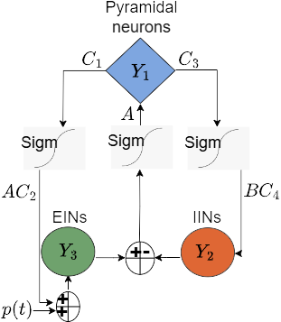
((a)) Block diagram Jansen-Rit model (1)

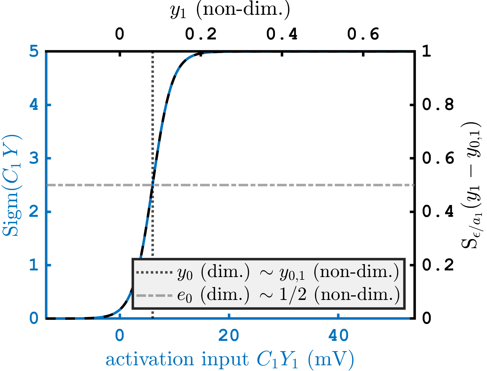
((b)) Profile of $\operatorname{S}$ (non-dim.) and $\operatorname{Sigm}$ (dim.)

Figure 1: (a) Interactions between $3$ neuronal populations in local circuit of a single cortical column in cerebral cortex of brain modelled by (1): pyramidal cells ($Y_{1}$) and excitatory ($Y_{3}$, EINs) and inhibitory ($Y_{2}$, IINs) interneurons. (b) Blue axis: Sigmoid profile of $\operatorname{Sigm}$, given in (2), with slope $r=0.56$ at threshold $y_{0}=6$ mV (vertical dotted line), at which half maximum $e_{0}$ of $\operatorname{Sigm}$ is achieved. (b) Black axis: dimensionless sigmoid $\operatorname{S}$, given in (6), for maximal slope value $a_{1}/4\epsilon=1/4(0.024)\approx 10$ at activation threshold $y_{0,1}=0.08$ (non-dimensionalised threshold $y_{0,1}$ for excitatory populations indicated by black vertical dotted line). See Table 1 and Table 2 for other parameters of $\operatorname{Sigm}$ and $\operatorname{S}$.

Figure 1(a) shows the structure of the Jansen-Rit model for a single cortical column. The model assumes that the cortical column contains two populations of interneurons, one excitatory and one inhibitory, and a population of excitatory pyramidal cells. The model contains two blocks for each population, a linear dynamic block, modelled as a second-order differential equation with the population’s average postsynaptic potential (PSP) $Y_{i}$ as its output and an average pulse density of action potentials as its input. In Fig. 1(a) these are the blocks with label $Y_{i}$: $Y_{1}$ is the PSP of the pyramidal cell population (blue diamond in Fig. 1(a)), $Y_{2}$ is the PSP of the inhibitory interneuron population (red ellipse in Fig. 1(a)), and $Y_{3}$ is the PSP of the excitatory interneuron population (green ellipse in Fig. 1(a)). The other block for each population is a nonlinear sigmoid-type activation function (the blocks labelled “Sigm” in Fig. 1(a)) from the PSP into an average pulse density of action potentials.

The arrows in Figure 1(a) show a positive feedback loop between the pyramidal neuron population ($Y_{1}$) and the excitatory interneuron population ($Y_{3}$), where both connections are excitatory; and a negative feedback loop between the pyramidal cells and the inhibitory interneurons ($Y_{2}$), where the connection back from the inhibitory neurons to the pyramidal cells is inhibitory. The model incorporates an external excitatory input, labelled $p(t)$ (an average pulse density) representing signalling from other neuronal populations external to the column (Fig. 1(a)). The resulting ODE system corresponding to the schematic diagram Fig. 1(a) is as follows (note the second order of each equation):

$$\begin{split}\ddot{Y}_{1}(t)&=Aa\{\operatorname{Sigm}(Y_{3}(t)-Y_{2}(t))\}-2a\dot{Y}_{1}(t)-a^{2}Y_{1}(t),\\ \ddot{Y}_{2}(t)&=Bb\{C_{4}\operatorname{Sigm}(C_{3}Y_{1}(t)\}-2b\dot{Y}_{2}(t)-b^{2}Y_{2},\\ \ddot{Y}_{3}(t)&=Aa\{p(t)+C_{2}\operatorname{Sigm}(C_{1}Y_{1}(t))\}-2a\dot{Y}_{3}(t)-a^{2}Y_{3}(t),\end{split}$$ (1)

where

$${\operatorname{Sigm}(Y)}=\frac{2e_{0}}{1+\mathrm{e}^{r(y_{0}-Y)}}$$ (2)

is a nonlinear sigmoid activation function, converting local field postsynaptic potential into firing rate, as shown in Fig. 1(b). Its argument $y$ is the average postsynaptic potential in mV of the neural population. The threshold $y_{0}$ determines the input level at which the firing rate is half of its maximum $2{e_{0}}$, and $r$ is the slope of $\operatorname{Sigm}$ at $y_{0}$.

We restrict our study mostly to the case without external input signal by setting the input $p(t)$ to zero, i.e. $p(t)=0$. In previous studies the values of $p(t)$ has been varied from 120 Hz to 320 Hz as proposed by Jansen and Rit [15]. For example, Grimbert and Fauregas (2006) [13] have performed bifurcation analysis of (1) varying the input $p(t)$.

Table 1: Quantities in Jansen-Rit model, (1), and their default values and dimensions[15].

Parameter	Description	Value/unit
$Y_{i}(t),i=1,3$	excitatory postsynaptic potential EPSP	mV
$Y_{2}(t)$	inhibitory postsynaptic potential IPSP	mV
$2e_{0}$	asymptotic maximum of $\operatorname{Sigm}$	$5\,\text{s}^{-1}$
$y_{0}$	switching threshold of $\operatorname{Sigm}$ ($\operatorname{Sigm}(y_{0})=e_{0}$)	$6\,[\text{mV}]^{-1}$
$r$	slope of $\operatorname{Sigm}$ at $y=y_{0}$ ($\operatorname{Sigm}^{\prime}(y_{0})$)	$0.56\,[\text{mV}]^{-1}$
$A$	maximal amplitude of excitatory PSP	$3.25\,\text{mV}$
$B$	maximal amplitude of inhibitory PSP	$22\,\text{mV}$
$a$	decay rate in excitatory populations	$100\,\text{s}^{-1}$
$b$	decay rate in inhibitory population	$50\,\text{s}^{-1}$
$\alpha_{i}$, $i=1,\ldots,4$	average number of synaptic connections	$\alpha_{1}=1,\alpha_{2}=0.8,\alpha_{3}=0.25$, $\alpha_{4}=0.25$
$C_{i}$, $i=1,\ldots,4$	connectivity strength	$C_{1}=135\alpha_{1},\ C_{2}=\alpha_{2}C_{1},\ C_{3}=\alpha_{3}C_{1},\ C_{4}=\alpha_{4}C_{1}$
$p$	External signal	0

The quantity $Y_{3}(t)-Y_{2}(t)$ can be related to experiments, because it is proportional to the signals obtained via EEG recordings corresponding to the average local field potential generated by the underlying neuronal populations in the cortical circuits [16]. In the cortex, pyramidal neurons project their apical dendrites into the superficial layers where the post-synaptic potentials are summed, thereby making up the core of the EEG. The interpretation of all model quantities and their numerical values and dimensions are given in Table 1. The values are set to those proposed by Jansen and Rit in [15].

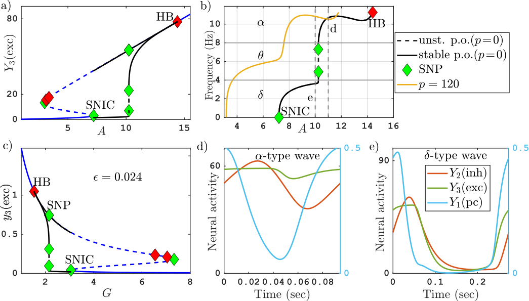
Figure 2: (a) Bifurcation diagram of Jansen-Rit model (1) for varying ${A}$; (b) frequency of oscillations with input ${p=0}$ (black) and input ${p=120}$ (yellow) for varying ${A}$, indicating alpha, theta and delta frequency ranges. (c) Bifurcation diagram of nondimensionalised Jansen-Rit model (5) for varying ratio of feedback strengths between inhibitory and excitatory neurons $G=B/A$. (d),(e) Time profiles of oscillations in alpha (${A=11}$) and delta (${A=10}$) rhythm regimes corresponding to 2 vertical dashed lines in panel b. For other parameters see Tables 1 and 2, computation performed with coco [6].

Sharp transitions from alpha to delta activity

Figure 2a shows the one-parameter bifurcation diagram of the Jansen and Rit model (1) for varying excitability scaling factor ${A}$, which determine maximal amplitude of excitatory postsynaptic potentials (EPSP) of excitatory populations (pyramidal cells $Y_{1}$) and exictatory interneurons ($Y_{3}$). All other parameters are fixed as listed in Table 3. The $y$-axis shows the PSP of the excitatory interneurons ($Y_{3}$). A branch of equilibria (blue) folds back and forth in two saddle node bifurcations (green diamonds). Solid curves are stable, dashed curves are unstable parts of the branch. Along the upper part of the branch the equilibria change stability in three Hopf bifurcation (red diamonds). We focus on the periodic orbits (oscillations) emerging from the Hopf bifurcation at a high value of ${A}$ (${A}\approx 15$, label (HB)). The black curves show the maximum and minimum values of $y_{3}$ along this branch of mostly stable periodic orbits that emanate from this Hopf bifurcation and terminate at the low-${A}$ end in a homoclinic bifurcation of saddle-node on invariant circle type (SNIC), at which the frequency of oscillation goes to zero as ${A}$ approaches the value for the saddle node bifurcation on the lower branch of equilibrium points (${A}\approx 7$).

Figure 2b shows the frequency of these oscillations over the range of parameters $A$ where they exist (${A}\in[7,14.4]$). We observe a sharp transition between high-frequency oscillations for $A$ in the range $[10.2,14.4]$ where the frequency (in Hz) is in the range $[8,11]$, and low-frequency oscillation for ${A}$ in the range $[7,10.2]$, where the frequency is about $4$ Hz and below. The oscillation frequencies on either side of the transition are associated with wakefulness state (alpha-like activity, $\approx 10$ Hz) and deep sleep (delta like activity, $\approx 2$ Hz).

Panels d and e in Figure 2 show that this change in frequency is accompanied with a qualitative change in the time profiles of the orbits. The alpha-type fast oscillations have a four-phase profile typical for an oscillatory negative feedback loop (compare Fig. 2d, and note that the scale of the outputs is different such that Fig. 2d has two $y$-axes):

• ($0$–$0.02$ s) high pyramidal cell output ($Y_{1}$, blue) causes rising inhibition ($Y_{2}$, red),

• ($0.02$–$0.05$ s) high inhibition causes decrease in pyramidal cell output,

• ($0.03-0.07$ s) low pyramidal cell output causes decreasing inhibition,

• ($0.06-0.1$ s) low inhibition causes rising pyramidal cell output.

Throughout the entire period of the alpha-type oscillation the pyramidal cell output is supported by a near-constant input from the excitatory interneurones ($Y_{3}$, green). The delta activity (slow) oscillations are shown in Fig. 2f. They show a relaxation-type time profile: pyramidal cell output $Y_{1}$ (blue) and excitatory interneuron output $Y_{3}$ (green) collapse to zero and stay there for some period. This period is determined by how long it takes for inhibition ($Y_{2}$, red) to reach sufficiently low levels to permit pyramidal cell output $Y_{1}$ and excitatory interneuron output $Y_{3}$ to rise again. The two time profiles in Fig. 2d and 2e occur for parameter values of $A$ just above (Figure 2d, $A=11$) and below (Figure 2e, $A=10$) the transition. The bifurcation diagram shows even a tiny region of bistability, bounded by two saddle-node-of-limit-cycle bifurcations. However, this bistability and the saddle-nodes are not a consistent feature for this transition. Figure 2b shows a bifurcation diagram for non-zero external input ($p=120$ Hz, yellow curve), where the transition still occurs and is still sharp, occurring in a small parameter region, but without bistability or saddle-nodes of limit cycles.

Forrester et al. [11] detected this transition in their investigation of the Jansen-Rit model (1). They demonstrated that it is an essential ingredient in the occurrence of large-scale oscillations in a network of neural populations (which would be measurable by EEG). As the transition is not associated with a bifurcation in parts of the parameter space (see Fig. 3 of [11]), the authors labelled the transition a “false bifurcation” and tracked it in parameter space by associating it with a feature of the time profile, namely the occurrence of an inflection point. Forrester et al. [11] pointed out that “false bifurcations” are usually originating from singular perturbation effects in the system, referring to Desroches et al. [8] and Rodrigues et al. [22].

To investigate this phenomenon further we non-dimensionalise the Jansen-Rit model (1) and identify a small parameter $\epsilon$ for which we can then study the singular limit for the transition from alpha to delta activity. Bifurcation diagram 2a shows a sharp change in the time profile of $Y_{3}$ from nearly constant for alpha activity to an oscillation with excursions close to zero: observe the drop in the minimum of the periodic orbit (black curve) for $A$ slightly above $10$.

The numerical bifurcation analysis of the Jansen-Rit model is carried out using the coco toolbox [6], which is a MATLAB-based platform for parameter continuation allowing for bifurcation analysis of equilibria and periodic orbits. Numerical continuation in coco [6] and xppaut [10] is used to track stability of equilibria and periodic orbits and to detect their bifurcations. For numerical integration (simulation), we use xppaut and ode45 (a Runge–Kutta method) in matlab. In all single-parameter bifurcation diagrams solid curves indicate stable states, while dashed lines are unstable states. Black curves indicate maximum and minimum values of periodic solutions in all bifurcation diagrams.

3 Singular perturbation analysis of Jansen-Rit model

We introduce small parameter $\epsilon>0$ for which in the limit $\epsilon\to 0$ the right-hand side (vector field) of system (1) becomes a non-smooth system. First we non-dimensionalise the Jansen-Rit model (1) to identify the small parameter.

Non-dimensionalisation of Jansen-Rit model (1)

Touboul et al. [24] present a non-dimensionalised version of the Jansen-Rit model. We choose the following dimensionless scale, as proposed by Touboul et al.[24]:

• Dimensionless time is set according to the internal decay time scale of the excitatory populations, $t_{\mathrm{new}}=at_{\mathrm{old}}$, where ${a}$ is given in Table 1.

• We introduce the decay rate ratio of inhibitory to excitatory populations ${b^{*}}$ and the ratio of postsynaptic amplitudes of inhibitory to excitatory populations

  $${b^{*}} =\frac{{b}}{{a}}, G =\frac{{B}}{{A}}.$$

• We rescale the state variables $Y_{1}$, $Y_{2}$, $Y_{3}$ such that they are all of order $1$ at their maximum, introducing a small parameter,

  $$\epsilon =\frac{2{a}}{{BrC(2e_{0})}}\approx 0.024$$ (3)

  $$y_{1}(t_{\mathrm{new}}) =rC\epsilon Y_{1}\left(\frac{t_{\mathrm{new}}}{a}\right),\ y_{2}(t_{\mathrm{new}})=r\epsilon Y_{2}\left(\frac{t_{\mathrm{new}}}{a}\right),\ y_{3}(t_{\mathrm{new}})=r\epsilon Y_{3}\left(\frac{t_{\mathrm{new}}}{a}\right).$$ (4)

We note that in Figure 2 e,f) $Y_{1}$ and $Y_{2}$, $Y_{3}$ are on different $y$-axes, because they have different orders of magnitude. The non-dimensionalisation (4) ensures that pyramidal cell output $y_{1}$ has the same (order-$1$) magnitude as the inhibitory interneurons ($y_{2}$) and the excitatory interneurons ($y_{3}$). The quantity $b^{*}$ is a measure of the difference in internal times scales between inhibitory and excitatory populations. Usually $b^{*}<1$ as inhibition is slower. The quantity $G$ is a measure for how strong internal feedback strength from inhibitory populations is compared to excitatory populations.

By substituting these dimensionless dependent variables into equation (1), and applying the chain rule with respect to the dimensionless time scale $t_{\mathrm{new}}$, we obtain the dimensionless form (using $\dot{y}_{i}$ and $\ddot{y}_{i}$ also for the new time)

$$\begin{split}\ddot{y}_{1}&=\frac{2}{G}\operatorname{S}_{\epsilon/a_{1}}\left(y_{3}-y_{2}-y_{0,1}\right)-2\dot{y}_{1}-y_{1},\\ \ddot{y}_{2}&=2b^{*}\alpha_{4}\operatorname{S}_{\epsilon/a_{2}}(y_{1}-y_{0,2})-2b^{*}\dot{y}_{2}-(b^{*})^{2}y_{2},\\ \ddot{y}_{3}&=\frac{P}{G}+\frac{2\alpha_{2}}{G}\operatorname{S}_{\epsilon/a_{3}}(y_{1}-y_{0,3})-2\dot{y}_{3}-y_{3},\\ \end{split}$$ (5)

where new dimensionless sigmoidal transformation is (see Fig. 1(b))

$${\operatorname{S}_{\epsilon}(y)}=\cfrac{1}{1+\exp\left(-y/\epsilon\right)}.$$ (6)

Table 2: Parameter values of the dimensionless model equation (5).

Parameter	Relation to the original parameters	Value
$\epsilon$	inverse of slope of activation function defined in formula 2	0.024
$y_{0,1},y_{0,2},y_{0,3}$	re-scaled activation thresholds	$y_{0,1}=y_{0,3}=0.08$, $y_{0,2}=0.3$
$G$	$B/A$ ratio of feedback strengths	$[0.5,20]$ (varied)
$b^{*}$	$b/a$ time scale ratio (inh. vs. exc.)	[0.2,0.5] (varied, original $0.5$)
$P$	$\epsilon Brp(t)/a$, external input	0
$\alpha_{2},\alpha_{4}$	average number of synaptic connections (same as original)	$\alpha_{2}=0.8$, $\alpha_{4}=0.25$
$a_{i}$	population-dependent factors in sigmoid slope	$a_{1}\!=\!a_{3}\!=\!1$, $a_{2}\!=\!1/4$.

As we have rescaled the PSP’s $Y_{i}(t)$, the thresholds in the activation function $\operatorname{S}$ are now different for each neuron population, such that we call them $y_{0,i}$. These thresholds $y_{0,i}$, at which the activation $\operatorname{S}_{\epsilon/a_{i}}(y-y_{0,i})$ equals $1/2$, now show up in (5). The new non-dimensional activation thresholds are

$$y_{0,1} =\frac{ry_{0}}{a_{1}}\epsilon, y_{0,2} =\frac{ry_{0}}{a_{2}}\epsilon, y_{0,3} =\frac{ry_{0}}{a_{3}}\epsilon,\mbox{\quad where $a_{1}=a_{3}=1$, $a_{2}=1/4$,}$$ (7)

using the parameters from Table 1, which result in the non-dimensional parameters shown in Table 2. Note that the main difference to Touboul’s non-dimensionalisation [24] is that the definition of the sigmoid function includes the scaling factor $\epsilon$.

Figure 2d shows the bifurcation diagram Figure 2a in the non-dimensionalised quantities. The new primary bifurcation parameter $G$ (the ratio of feedback strengths between inhibition and excitation) is proportional to the inverse of the excitation feedback strength $A$, such that now the alpha-to-delta frequency transition occurs for increasing $G$ at $G\approx 2.2$. The Hopf bifurcation occurs for low $G\approx 1.5$ and the SNIC connecting orbit occurs at $G\approx 3.2$.

In the non-dimensionalised model (6) the small parameter $\epsilon$, which equals $0.024$, appears in the inverse of the slope of the dimensionless sigmoid $\operatorname{S}_{\epsilon}$ at $y=0$ letting the sigmoid $\operatorname{S}_{\epsilon}$ approach a discontinuous switch in the limit for small $\epsilon$ and $i=1,2,3$:

$$\lim_{\epsilon\to 0}\operatorname{S}_{\epsilon}(y-y_{0,i}) =\begin{cases}0&\mbox{if $y<y_{0,i}$,}\\ 1&\mbox{if $y>y_{0,i}$,}\end{cases}$$ (8)

In addition the activation thresholds $y_{0,i}$ inherit a factor $\epsilon$ in (7). However, we observe that there are non-trivial factors in front of $\epsilon$ in several places. Since the $\epsilon$ in the original parameters setting is about $1/40$ (so not that small), these factors will influence our strategies for taking the singular limit $\epsilon\to 0$.

• The slope in the activation for the inhibitory interneurons, $S_{\epsilon/a_{2}}$, is $a_{2}/4\epsilon=1/(16\epsilon)\approx 2.6$. So, it is further away from the limiting discontinuous switch than the activation of the excitatory populations.

• The factors $ry_{0}/a_{1}$ and $ry_{0}/a_{3}$ are such that $y_{0,1}=y_{0,3}\approx 0.08$, such that the activation thresholds are small, but not as small as $\epsilon$.

• The factor $ry_{0}/a_{2}$ is such that $y_{0,2}\approx 0.3$, such that $y_{0,2}$ is not a small quantity.

The smallness of $\epsilon$ expresses that the internal dynamics of neurons in the excitatory populations is fast, leading to small thresholds and steep activation functions. The inhibitory neural population is comparatively slower, leading at the population level to a shallower slope of the activation curve and a larger activation threshold [27]. The above observations suggest several possible singular limits.

(a)

We let $\epsilon$ go to zero in the denominator appearing in $\operatorname{S}_{\epsilon/a_{i}}$ for all neuron populations ($i=1,2,3$) simultaneously. At the same time we keep the activation thresholds $y_{0,i}$ fixed for all populations. This leaves the parameters $y_{0,i}$ in the model as independent parameters and uses the concrete values from Table 2.

(b)

We let $\epsilon$ go to zero in the denominator appearing in $\operatorname{S}_{\epsilon/a_{i}}$ for all neuron populations ($i=1,2,3$) simultaneously, and we let the activation thresholds $y_{0,1}$ and $y_{0,3}$ for the excitatory neuron populations go to zero (either proportional to $\epsilon$ or at some lower rate).

(c)

We let $\epsilon$ go to zero for the excitatory neurons populations ($i=1,3$) in the slope of the activations $\operatorname{S}_{\epsilon/a_{i}}$, but keep the activation for the inhibition with a fixed finite slope, equal to $\approx 10$ (as well as keeping the activation threshold $y_{0,2}\approx 0.3$ fixed).

We will focus in our analysis on strategies (a) and (b), because they permit explicit expressions for most equilibria and their bifurcations. They also result in an implicit algebraic condition for the alpha-to-delta transition. In both limits the collapse of the alpha-frequency oscillations is a grazing bifurcation [9] of periodic orbits in a piecewise linear ODE. In limit (a) the collapse leads to a low excitation equilibrium ($y_{i}\ll 1$ for $i=1,2,3$), in limit (b) it leads to delta activity.

In the numerical bifurcation diagram in Fig. 2d the three boundaries for alpha and delta activity are the Hopf bifurcation (onset of alpha frequency oscillations) at $G\approx 1.5$, the transition between alpha and delta activity at $G\approx 2.2$ and the connecting orbit to a saddle-node at $G\approx 3.2$. Two of the boundaries can be found by analysis of equilibria, namely the Hopf bifurcation and the saddle-node bifurcation for small $y_{i}$.

For our analysis, the dimensionless external input $p$ is fixed to zero. We use the dimensionless parameter $G$ (the ratio between feedback strength of inhibition versus excitation) as our primary bifurcation parameter. We will later vary $b^{*}$, the ratio between internal time scales between inhibition and excitation as a secondary bifurcation parameter.

3.1 Equilibrium analysis in the small-$\epsilon$ limit

Inserting $\epsilon=0$ (or $\epsilon\ll 1$) into the activation functions in (5) and (6), results in an easy-to-interpret limit for equilibria. Setting all derivatives in equation (5) to zero, we obtain that the equilibrium values for $y_{1}$, $y_{2}$, $y_{3}$ satisfy the algebraic equations

$$y_{1} =\frac{2}{G}\operatorname{S}_{\epsilon}(y_{3}-y_{2}-y_{0,1})$$ (9)

$$y_{2} =\frac{2\alpha_{4}}{b^{*}}\operatorname{S}_{\epsilon/a_{2}}(y_{1}-y_{0,2})$$ (10)

$$y_{3} =\frac{2\alpha_{2}}{G}\operatorname{S}_{\epsilon}(y_{1}-y_{0,3}).$$ (11)

The right-hand sides of (10) and (11) define the equilibrium values $y_{2}$ and $y_{3}$ as a function of $y_{1}$. This is also true in the limit $\epsilon=0$, whenever $y_{1}$ is not on the activation threshold ($y_{0,2}$ and $y_{0,3}$, respectively).

Inserting (10) and (11) into (9) and taking the Heaviside limit $S_{0}$ in (8) for the activation functions $S_{\epsilon/a_{i}}$ (indicating the dependence of $y_{2}$ and $y_{3}$ on $y_{1}$), leads to the relation

$$\frac{G}{2}y_{1}=\operatorname{Rhs}_{0}(y_{1}):=\begin{cases}0&\mbox{if $y_{3}(y_{1}-y_{03})-y_{2}(y_{1}-y_{02})<y_{01}$,}\\ 1&\mbox{if $y_{3}(y_{1}-y_{03})-y_{2}(y_{1}-y_{02})>y_{01}$,}\end{cases}$$ (12)

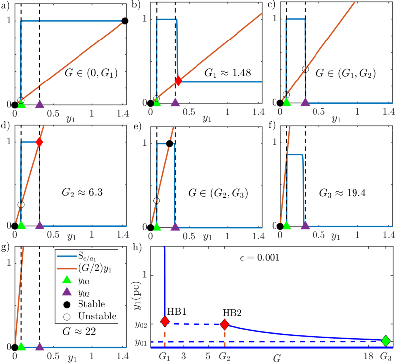
Figure 3: (a-g) Intersections between left- (red) and right-hand (blue) side of (12) for different bifurcation parameters $G$ (plots used $\epsilon=0.001$, $y_{0,1},y_{0,3}=0.08$ and $y_{0,2}=0.3$). (h) Numerical bifurcation diagram of equilibria in $(G,y_{1})$-plane obtained by coco [6]. $\operatorname{S}_{\epsilon}/a_{1}=\operatorname{S}_{\epsilon}(y_{3}-y_{2}-y_{0,1})$ for $y_{1}$ in equation (9). For other parameters see Table 2.

Table 3: Equilibrium points present in system (5) for all parameter ranges of $G$: for critical values of $G$ see (13), (14). The index is the number of unstable eigenvalues of the Jacobian in the equilibrium for non-zero $\epsilon$.

range of $G$	Fig. 3 panel	equilibrium location	index
$I_{1}=(0,G_{1})$	(a)	$y_{\mathrm{eq_{1}}}=(0,0,0)$	$0$
		$y_{\mathrm{eq_{2}}}=(y_{0,3},0,y_{0,1})$	$1$
		$y_{\mathrm{eq_{3}}}=(2/G,2\alpha_{4}/b^{*},2\alpha_{2}/G)$	$0$
$G_{1}$: Hopf bifurcation	(b)
$I_{2}=(G_{1},G_{2})$	(c)	$y_{\mathrm{eq_{1}}}=(0,0,0)$	$0$
		$y_{\mathrm{eq_{2}}}=(y_{0,3},0,y_{0,1})$	$1$
		$y_{\mathrm{eq_{4}}}=(y_{0,2},2\alpha_{2}/G-y_{0,1},2\alpha_{2}/G)$	$2$
$G_{2}$: Hopf bifurcation	(d)
$I_{3}=(G_{2},\min(G_{3},G_{4}))$	(e)	$y_{\mathrm{eq_{1}}}=(0,0,0)$	$0$
		$y_{\mathrm{eq_{2}}}=(y_{0,3},0,y_{0,1})$	$1$
		$y_{\mathrm{eq_{4}}}=(2/G,0,2\alpha_{2}/G)$	$0$
$\min(G_{3},G_{4})$: saddle-node	(f)
$I_{4}=(\min(G_{3},G_{4}),\infty)$	(g)	$y_{\mathrm{eq_{1}}}=(0,0,0)$	$0$

Analysis of (9)–(11) in the limit $\epsilon\to 0$ is supported by Figure 3. Each panel shows the left-hand side of (12) (in red) and the right-hand side $\operatorname{Rhs}_{0}(y_{1})$ of (12) (in blue) as a function of $y_{1}$ for different values of $G$, otherwise using the parameter values in Table 2. The (red) left-side function is the straight line $y_{1}\mapsto Gy_{1}/2$. The right-side function $\operatorname{Rhs}_{0}(y_{1})$ is piecewise constant. Defining two critical values for parameter $G$ as

$$G_{1} =\frac{\alpha_{2}b^{*}}{\alpha_{4}+y_{0,1}b^{*}/2}\approx 1.48, G_{3} =\frac{2\alpha_{2}}{y_{0,1}}\approx 19.4,$$ (13)

(thus, $0<G_{1}<G_{3}$) the right-hand side $\operatorname{Rhs}_{0}$ has the values (recall that $0<y_{0,3}<y_{0,2}$)

$$\begin{aligned} \\ \operatorname{Rhs}_{0}(y_{1})&=\begin{cases}\\ \\ \ \end{cases}\end{aligned}\begin{aligned} &&\mbox{for $G$ in:}&&(0,&G_{1}),&(G_{1},&G_{3}),&(G_{3},&\infty),\\ y_{1}&\in(0,y_{0,3})&\mbox{($y_{2}$ off, $y_{3}$ off):}&&&0&&0&0\\ y_{1}&\in(y_{0,3},y_{0,2})&\mbox{($y_{2}$ off, $y_{3}$ on):}&&&1&&1&0\\ y_{1}&\in(y_{0,2},\infty)&\mbox{($y_{2}$ on, $y_{3}$ on):}&&&1&&0&0\\ \end{aligned}$$

Each intersection of the two lines in Fig. 3 is a stable equilibrium if $\operatorname{Rhs}_{0}$ (blue line) is horizontal in the intersection, or an unstable pseudo-equilibrium [18, 9], if $\operatorname{Rhs}_{0}$ is vertical in the intersection. For $\epsilon\ll 1$ but non-zero, the pseudo-equilibria of the piecewise linear limit system will become unstable equilibria with strongly unstable eigenspaces. Table 3 lists the locations of equilibria for all ranges of parameter $G$, with two additional critical values for $G$,

$$G_{2} =\frac{2}{y_{0,2}}\approx 6.3, G_{4} =\frac{2}{y_{0,3}}\approx 24.8.$$ (14)

Figure 3h shows the resulting bifurcation diagram in the limit of small $\epsilon$.

Figure 3a shows that for $G<G_{1}$ we have a pair of a stable and unstable equilibria with $y_{1}$ near $0$, where the saddle is has $y_{1}=y_{0,3}$, and the node is very close to zero $\sim\exp(-y_{0,1}/\epsilon)$). Another stable equilibrium exists with large $y_{1}$, equal to $2/G$. At $G=G_{1}$ (Fig. 3b, see (13) for value of $G_{1}$) $\operatorname{Rhs}_{0}$ drops to zero for $y>y_{0,2}$, which results in a sudden drop of the $y_{1}$-component of the large-$y_{1}$ equilibrium to $y_{0,2}$ and its loss of stability. For positive $\epsilon$ this loss of stability is a Hopf bifurcation (see the labeled point HB1 in Fig. 3h). Figure 3c shows the equilibria for $G>G_{1}$. The situation at the next critical $G=G_{2}=2/y_{0,2}$ is shown in Fig. 3d, when the left-hand side function (red line) goes through the “corner” of $\operatorname{Rhs}_{0}$ at $y_{1}=y_{0,2}$. At this value the equilibrium with $y_{1}=y_{0,2}$ regains its stability in a Hopf bifurcation for non-zero $\epsilon$ (see the labeled point HB2 in Fig. 3h). Fig. 3e shows the situation for $G>G_{2}$ with two stable equilibria and one saddle. The next critical $G$ is $\min(G_{3},G_{4})$, when either the excitatory interneuron activity is no longer sufficient to overcome the threshold ($G_{3}$, when the blue line in Fig. 3g drops to zero on the $y_{1}$-interval $(y_{0,3},y_{0,2})$), or the left-hand side (red curve) touches the “corner” of $\operatorname{Rhs}_{0}$ at $y_{1}=y_{0,3}$ ($G_{4}$). In both cases, the resulting equilibrium bifurcation is a saddle-node bifurcation of the equilibrium with $y_{1}=y_{0,3}$ (see the labeled SN in Fig. 3h). For the parameters we study, we have that $G_{3}<G_{4}$ such that $G_{4}$ does not change the dynamics.

The case of small excitatory activation thresholds $y_{0,1}$ and $y_{0,3}$

If we assume proportionally small excitatory activation thresholds $y_{01}=y_{03}\sim\epsilon$, then the saddle and node equilibria with $y_{1}\approx 0$ are no longer present for any $G$ of order $1$. This follows immediately from a perturbation analysis of the equilibria for small non-zero $\epsilon$ and excitatory activation thresholds of the form

$$y_{0,1} =\epsilon z_{0,1}, y_{0,3} =\epsilon z_{0,3}, z_{0,1},z_{0,3} >0, z_{0,1},z_{0,3} =O(1).$$

Let us assume that $y_{1,\mathrm{eq}}\ll 1$, in particular, $y_{1,\mathrm{eq}}\ll y_{0,2}$ and check that no such equilibrium can exist. The smallness of $y_{1,\mathrm{eq}}$ together with identity (10), $y_{2,\mathrm{eq}}=2\alpha_{4}/(b^{*}(1+\exp((y_{0,2}-y_{1,\mathrm{eq}})/(\epsilon/a_{2})))$, would imply that the corresponding inhibitory interneuron activity $y_{2,\mathrm{eq}}$ is very close to zero: $y_{2,\mathrm{eq}}\sim\exp(-y_{0,2}/\epsilon)\leq\epsilon$. From this, the identities (9) and(11) imply positive lower bounds independent of $\epsilon$ for the equilibrium pyramidal-cell activity $y_{1,\mathrm{eq}}$ and the excitatory interneuron activity $y_{3,\mathrm{eq}}$, namely

$$y_{1,\mathrm{eq}} \geq\frac{2}{G}\frac{1}{1+\exp(z_{0,1}+y_{2,\mathrm{eq}}/\epsilon)}\geq\frac{2}{G}\frac{1}{1+\exp(z_{0,1}+1)}, y_{3,\mathrm{eq}} \geq\frac{2\alpha_{2}}{G}\frac{1}{1+\exp(z_{0,3})}$$ (15)

Hence, for excitatory activation thresholds of order $\epsilon$ the pair of small-$y_{1}$ equilibria does not exist. The other equilibria in Table 3 and Fig. 3h have well-defined limits for $y_{0,1},y_{0,3}\to 0$: the stable equilibrium has the limit $y_{1}=2/G$, the unstable equilibrium has the limit $y_{1}=y_{0,2}$ and its inhibitory activity $y_{2}$ approaches $2\alpha_{2}/G$ for small $y_{0,1}$. The saddle-node bifurcation at $\min(G_{3},G_{4})$ goes to infinity as $y_{0,1},y_{0,3}\to 0$, such that the large-activity equilibrium exists over a wider range of $G$. This leaves the region $(G_{1},G_{2})$ between the two Hopf bifurcations, where no stable equilibrium exists for $y_{0,1},y_{0,3}$ of order $\epsilon$. The Hopf bifurcation at $G_{1}$ has the limit $\alpha_{2}b^{*}/\alpha_{4}$ for $y_{0,1}\to 0$, while $G_{2}$ is independent of $y_{0,1}$ and $y_{0.3}$.

3.2 Piecewise exponential periodic orbits in the small-$\epsilon$ limit

Absence of sliding

System (5) in the limit $\epsilon\to 0$ has discontinuities on the right-hand side such that it is of Filippov type [9]. However, the structure of (5) rules out phenomena such as sliding. In the hyperplanes where the vector field is discontinuous, the two half-space vector fields point into the same direction relative to the hyperplane. This is due to the presence of inertia: (5) is a system of second-order equations for the firing activities but the switches in $\operatorname{S}_{0}$ depend only on the firing activities, not their time derivatives. Let us inspect each discontinuity set:

• $D_{i}=\{y:y_{1}=y_{0,i}\}$ for $i=2,3$: the inner product of the vector fields $\dot{y}$ with the perpendicular of $D_{i}$, $D_{i}^{\bot}$ on both sides $D_{i}$ equals $\dot{y}_{1}$, which is continuous across $D_{i}$ and, thus, all non-equilibrium trajectories cross the surface $D_{i}$ in the same direction from both sides of $D_{i}$.

• $D_{1}=\{y:y_{3}-y_{2}=y_{0,1}\}$: the inner product of $\dot{y}$ with $D_{1}^{\bot}$ is $\dot{y}_{3}-\dot{y}_{2}$, and is also continuous across $D_{1}$.

• $D_{1,i}=\{y:y_{1}=y_{0,i}\mbox{\ and\ }y_{3}-y_{2}=y_{0,1}\}$ for $i=2,3$: By the above two observations along this codimension-$2$ discontinuity surface, trajectories always point into the same hyper-quadrant from all $4$ adjacent hyper-quadrants.

Hence, all non-equilibrium trajectories of system (5) are well defined in the classical sense.

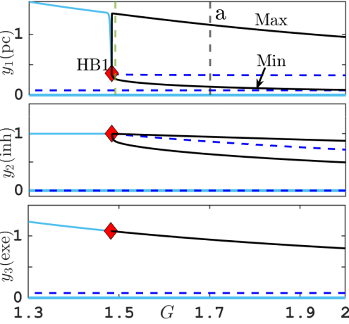
Figure 4: Continuation of equilibria and periodic orbits for three neural activity $y_{1},y_{2},y_{3}$ branching off Hopf bifurcation (HB1) for small $\epsilon=0.001$, respectively. Max and Min representing the maximum and minimum periodic orbit associated with parameter $G$. Green vertical line corresponding to canard orbit (see Fig 7) and grey vertical line corresponding to parameter $G=1.7$, where this value used in singular limit in Fig 5 panel (a). Other parameters are listed in Table 2

Piecewise linear oscillations in a negative feedback loop between pyramidal cells and inhibition for $\epsilon=0$

As seen in Table 3 and Figure 3h and Figure 4, in the small-$\epsilon$ limit the high-activity equilibrium $y_{1}$ changes not only its stability at $G=G_{1}$ but also its location: the equilibrium pyramidal-cell activity drops sharply from $y_{1}=2/G=2/G_{1}\approx 1.35$ to $y_{1}=y_{0,2}\approx 0.3$. Hence, in the singular limit we cannot expect the standard Hopf bifurcation scenario with a family of nearly harmonic small-amplitude periodic orbits branching off. First, we note that for $G\approx G_{1}$ and pyramidal-cell activity $y_{1}$ in the range between $y_{0,2}$ and $2/G_{1}$ the excitatory interneurons are uniformly active as $y_{1}$ is always above the threshold $y_{0,3}$ at which excitatory interneuron activity is switched off, and which is much smaller than $y_{0,2}$. Hence, $y_{3}$ will be positive and at its equilibrium value

$$y_{3}(t)\approx y_{3,\mathrm{eq}}=\frac{2\alpha_{2}}{G}\approx\frac{2\alpha_{2}}{G_{1}}=y_{0,1}+\frac{2\alpha_{4}}{b^{*}}.$$

Thus, we may replace $y_{3}$ in the sigmoid input for $y_{1}$ with its equilibrium value, resulting in the four-dimensional system for pyramidal-cell and inhibitory activity only, inserting the limit $\epsilon=0$:

$$\mbox{(if\ }y_{1}(t) >y_{0.3}\mbox{ for all time)}$$

$$\ddot{y}_{1} =(2/G)\,u_{1}-2\dot{y}_{1}-y_{1},$$ (16)

$$\ddot{y}_{2} =2b^{*}\alpha_{4}\ u_{2}-2b^{*}\dot{y}_{2}-(b^{*})^{2}y_{2}\mbox{,\quad where}$$ (17)

$$u_{1}(t) =\begin{cases}1&\mbox{if $y_{2}<2\alpha_{2}/G-y_{0,1}$,}\\ 0&\mbox{if $y_{2}>2\alpha_{2}/G-y_{0,1}$,}\end{cases}\quad u_{2}(t)=\begin{cases}0&\mbox{if $y_{1}<y_{0,2}$,}\\ 1&\mbox{if $y_{1}>y_{0,2}$.}\end{cases}$$

System (16), (17) is a classical negative feedback loop with inertia: $y_{2}$ suppresses $y_{1}$, while $y_{1}$ promotes $y_{2}$. Each oscillation period has four phases and follows a piecewise linear second-order vector field in each of the phases.

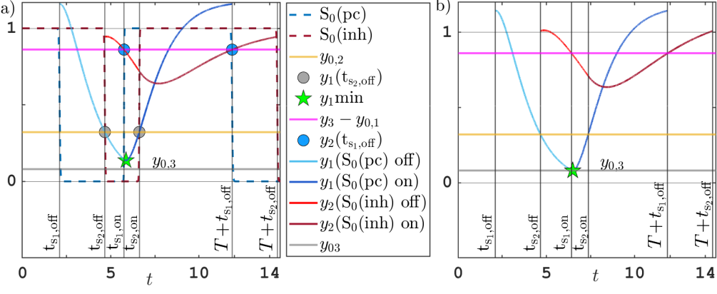
Figure 5: Time profile of alpha-type piecewise exponential periodic orbits given in (24) for $y_{0,1},y_{0,3}=0.08$ and $y_{0,2}=0.3$. The potential $y_{3}$ of excitatory interneurons $y_{3}$ is constant ($2\alpha_{2}/G$). Panel (a) shows orbit for $(b^{*},G)=(0.5,1.7)$. At $t_{\mathrm{s_{2},off}}$, $t_{\mathrm{s_{2},on}}$ $y_{1}$ crosses the threshold $y_{0,2}$ (yellow horizontal line), marked by grey filled circles, while blue filled circles indicate points at which $y_{2}$ crosses $y_{3}-y_{0,1}$ (magenta horizontal line) at $t_{\mathrm{s_{1},off}}$, $t_{\mathrm{s_{1},on}}$. Legend entry $S_{0}$(pc) is activation $\operatorname{S}_{0}\left(y_{3}-y_{2}(t)-y_{0,1}\right)$ for $y_{1}$ (indicated by dashed blue line), and $S_{0}$(inh) is activation $\operatorname{S}_{0}\left(y_{1}(t)-y_{0,2}\right)$ for $y_{2}$ (dashed red line). Panel (b) shows grazing orbit for $(b^{*},G)=(0.44,1.7)$, where $y_{1,\min}=y_{0,3}$, highlighted by green star on the grey horizontal line $\{y=y_{0,3}\}$ with time of switch (vertical dashed lines) of activation. For other parameters see Table 2.

Figure 5a shows the typical shape for the $y_{1}$ and $y_{2}$ profile of the oscillations. We reduce the periodic problem for the four-dimensional ODE to a four-dimensional algebraic problem, parametrising the oscillations using the times at which the respective activations $u_{1},u_{2}$ switch between $0$ and $1$ (w.l.o.g. $t_{\mathrm{s_{1},off}}=0$), see Figure 5a for guidance:

$$t_{\mathrm{s_{1},off}} =0<t_{\mathrm{s_{2},off}}<t_{\mathrm{s_{1},on}}<t_{\mathrm{s_{2},on}}<T\mbox{,\quad where}$$ (18)

$$t_{\mathrm{s_{1},off}}: y_{2} 2\alpha_{2}/G-y_{0,1} u_{1}:1\to 0$$    crosses from below to above, (),

$$t_{\mathrm{s_{2},off}}: y_{1} y_{0,2} u_{2}:1\to 0$$    crosses from above to below, (),

$$t_{\mathrm{s_{1},on}}: y_{2} 2\alpha_{2}/G-y_{0,1} u_{1}:0\to 1$$    crosses from above to below, (),

$$t_{\mathrm{s_{2},on}}: y_{1} y_{0,2} u_{2}:0\to 1$$    crosses from below to above, (),

$$T:$$    period of oscillation.

Canard explosion near Hopf bifurcation in singular limit

We observe from initial numerical bifurcation analysis for small $\epsilon$ ($\epsilon=0.001$, see Fig. 4) that the pyramidal-cell ($y_{1}$) amplitude for the family of periodic orbits emerging from the Hopf bifurcation grows over a small range of $G$ to order $1$, while the inhibition ($y_{2}$) amplitude grows square-root-like with $G-G_{1}$, as expected at a classical Hopf bifurcation (see Figure 5b).

Alpha-type oscillations in the singular limit

For $G>G_{1}$ the periodic orbits consist of two coupled pairs of orbit segments, one pair of segments for pyramidal activity $y_{1}$ (switching at times $t_{\mathrm{s_{1},off}}$ and $t_{\mathrm{s_{1},on}})$, and one pair of segments for inhibition $y_{2}$ (switching at times $t_{\mathrm{s_{2},off}}$ and $t_{\mathrm{s_{2},on}}$), as shown in Figure 5a. The coupling occurs through the switching times, as the switching times $t_{\mathrm{s_{2},on/off}}$ are determined by $y_{1}$ crossing the threshold $y_{0,2}$, and the switching times $t_{\mathrm{s_{1},on/off}}$ are determined by $y_{2}$ crossing the threshold $y_{\mathrm{3,eq}}-y_{0,1}=2\alpha_{2}/G-y_{0,1}$. The general solution $(y(t),\dot{y}(t))\in\mathbb{R}^{2}$ of the affine ODE IVP

$$\ddot{y} =b^{2}c-2b\dot{y}-b^{2}y,\quad(y(0),\dot{y}(0))=(y_{0},\dot{y}_{0})\in\mathbb{R}^{2},$$ (19)

with inhomogeneity $c$ is

$$Y_{\mathrm{adv}}\left(t;b,c,\begin{bmatrix}y_{0}\\ \dot{y}_{0}\end{bmatrix}\right)=\begin{bmatrix}y(t)\\ \dot{y}(t)\end{bmatrix}: =\operatorname{e}^{M_{b}t}\begin{bmatrix}y_{0}\\ \dot{y}_{0}\end{bmatrix}+\left[I_{2}-\operatorname{e}^{M_{b}t}\right]\operatorname{e}_{1}c\mbox{,\quad where\ }$$

$$\operatorname{e}^{M_{b}t} =\operatorname{e}^{-bt}\begin{bmatrix}1+bt&t\\ -b^{2}t&1-bt\end{bmatrix}\mbox{,}$$

and $\operatorname{e}_{i}$ are standard basis vectors. From this general formula we find that requiring periodicity of the pyramidal activity $y_{1}$ and the inhibition $y_{2}$ determines their initial conditions at the “off” switching time. The initial conditions

$$\begin{bmatrix}y_{1}(t_{\mathrm{s_{1},off}})\\ \dot{y}_{1}(t_{\mathrm{s_{1},off}})\end{bmatrix} =\frac{2}{G}Y_{\mathrm{per}}(T,t_{\mathrm{s_{1},on}}-t_{\mathrm{s_{1},off}};1),\ \begin{bmatrix}y_{2}(t_{\mathrm{s_{2},off}})\\ \dot{y}_{2}(t_{\mathrm{s_{2},off}})\end{bmatrix}=\frac{2\alpha_{4}}{b^{*}}Y_{\mathrm{per}}(T,t_{\mathrm{s_{2},on}}-t_{\mathrm{s_{2},off}};b^{*})\mbox{\ with}$$

$$Y_{\mathrm{per}}(T,\delta_{t};b) =\left[I_{2}-\operatorname{e}^{M_{b}T}\right]^{-1}\left[I_{2}-\operatorname{e}^{M_{b}(T-\delta_{t})}\right]\operatorname{e}_{1}\mbox{}$$

will lead to a solution of (16), (17) that is periodic with period $T$. The switching times $t_{\mathrm{s_{1},on}}$, $t_{\mathrm{s_{2},on/off}}$ and the period $T$ satisfy $4$ relations that follow from the crossing conditions $y_{1}(t_{\mathrm{s_{2},off}})=y_{1}(t_{\mathrm{s_{2},on}})=y_{02}$ and $y_{2}(t_{\mathrm{s_{1},off}})=y_{2}(t_{\mathrm{s_{1},on}})=y_{3}-y_{01}$:

$$\begin{array}[]{rcllccl}y_{0,2}&=&\operatorname{e}_{1}^{\mathsf{T}}Y_{\mathrm{adv}}(t_{\mathrm{s_{2},off}};&1,0,(\cdot))&\circ&(2/G)&Y_{\mathrm{per}}(T,t_{\mathrm{s_{1},on}}-t_{\mathrm{s_{1},off}};1)\\[2.15277pt] y_{0,2}&=&\operatorname{e}_{1}^{\mathsf{T}}Y_{\mathrm{adv}}(t_{\mathrm{s_{2},on}}-T;&1,2/G,(\cdot))&\circ&(2/G)&Y_{\mathrm{per}}(T,t_{\mathrm{s_{1},on}}-t_{\mathrm{s_{1},off}};1)\\[2.15277pt] \frac{2\alpha_{2}}{G}-y_{0,1}&=&\operatorname{e}_{1}^{\mathsf{T}}Y_{\mathrm{adv}}(t_{\mathrm{s_{1},on}}-t_{\mathrm{s_{2},off}};&b^{*},0,(\cdot))&\circ&(2\alpha_{4}/b^{*})&Y_{\mathrm{per}}(T,t_{\mathrm{s_{2},on}}-t_{\mathrm{s_{2},off}};b^{*})\\[2.15277pt] \frac{2\alpha_{2}}{G}-y_{0,1}&=&\operatorname{e}_{1}^{\mathsf{T}}Y_{\mathrm{adv}}(-t_{\mathrm{s_{2},off}};&b^{*},2\alpha_{4}/b^{*},(\cdot))&\circ&(2\alpha_{4}/b^{*})&Y_{\mathrm{per}}(T,t_{\mathrm{s_{2},on}}-t_{\mathrm{s_{2},off}};b^{*}).\end{array}$$ (24)

In (24) and below we use the composition symbol $\circ$ with the meaning $f\circ x=f(x)$, $f\circ g\circ x=f(g(x))$ etc. to reduce nesting of brackets. Recall that we set $t_{\mathrm{s_{1},off}}=0$ such that this switching time has been omitted in the defining equations (24). We have already inserted the appropriate initial conditions to ensure periodicity with period $T$ into (24), such that the system (24) is a system of $4$ algebraic equations, depending on the $4$ unknown times $t_{\mathrm{s_{1},on}}$, $t_{\mathrm{s_{2},off}}$, $t_{\mathrm{s_{2},on}}$ and $T$, and system parameters such as $G$, $b^{*}$ and the switching thresholds $y_{0,1},y_{0,2}$. For given switching times and period, one may obtain the complete periodic orbit as

$$\begin{bmatrix}y_{1}(t)\\ \dot{y}_{1}(t)\end{bmatrix} =Y_{\mathrm{adv}}\left(t;1,\frac{2}{G}u_{1}(t),(\cdot)\right)\circ\frac{2}{G}Y_{\mathrm{per}}(T,t_{\mathrm{s_{1},on}}-t_{\mathrm{s_{1},off}};1)\mbox{\quad for $t\in[t_{\mathrm{s_{1},on}}-T,t_{\mathrm{s_{1},on}}]$}$$

$$\begin{bmatrix}y_{2}(t)\\ \dot{y}_{2}(t)\end{bmatrix} =\begin{multlined}Y_{\mathrm{adv}}\left(t-t_{\mathrm{s_{2},off}};b^{*},\frac{2\alpha_{4}}{b^{*}}u_{2}(t),(\cdot)\right)\circ\frac{2\alpha_{4}}{b^{*}}Y_{\mathrm{per}}(T,t_{\mathrm{s_{2},on}}-t_{\mathrm{s_{2},off}};b^{*})\\ \mbox{for $t\in[t_{\mathrm{s_{2},on}}-T,t_{\mathrm{s_{2},on}}]$}\end{multlined}Y_{\mathrm{adv}}\left(t-t_{\mathrm{s_{2},off}};b^{*},\frac{2\alpha_{4}}{b^{*}}u_{2}(t),(\cdot)\right)\circ\frac{2\alpha_{4}}{b^{*}}Y_{\mathrm{per}}(T,t_{\mathrm{s_{2},on}}-t_{\mathrm{s_{2},off}};b^{*})\\ \mbox{for $t\in[t_{\mathrm{s_{2},on}}-T,t_{\mathrm{s_{2},on}}]$}$$

$$\begin{bmatrix}y_{3}(t)\\ \dot{y}_{3}(t)\end{bmatrix} \!=\!\begin{bmatrix}2\alpha_{2}/G\\ 0\end{bmatrix}$$

where $$\ u_{1}(t)=\begin{cases}0&\mbox{if $t\in[0,t_{\mathrm{s_{1},on}}]$}\\ 1&\mbox{if $t\in[t_{\mathrm{s_{1},on}}-T,0]$},\end{cases}\quad u_{2}(t)=\begin{cases}0&\mbox{if $t\in[t_{\mathrm{s_{2},off}},t_{\mathrm{s_{2},on}}]$}\\ 1&\mbox{if $t\in[t_{\mathrm{s_{2},on}}-T,t_{\mathrm{s_{2},off}}]$.}\end{cases}$$

Figure 5a shows an example of such a piecewise exponential and its switching times. The associated thresholds $y_{2}(t)=y_{\mathrm{3,eq}}-y_{0,1}=2\alpha_{2}/G-y_{0,1}$ and $y_{1}(t)=y_{0,2}$ for the switching events are shown magenta and yellow horizontal lines, respectively.

Detection of grazing boundary for alpha activity

The orbits given by algebraic system (24) are alpha activity oscillations with constant support by excitatory interneuron population $y_{3}$. A criterion for the existence of these oscillations is that $y_{1}$ never crosses below the threshold $y_{0,3}$ at which the excitatory interneurons $y_{3}$ switch off. The piecewise exponential has a distinct minimum $y_{1,\min}$ at some time $t_{1,\min}$, labelled by a star in Figure 5a. This minimum consistently occurs shortly after $t_{\mathrm{s_{1},on}}$, in the interval between $t_{\mathrm{s_{1},on}}$ and $t_{\mathrm{s_{2},on}}$, due to the inertia caused by the second-order nature of the ODE for $y_{1}$. Hence, we may introduce $y_{1,\min}$ and $t_{1,\min}$ as additional parameters satisfying the relations

$$\begin{bmatrix}y_{1,\min}\\ 0\end{bmatrix} =\begin{multlined}Y_{\mathrm{adv}}(t_{1,\min}-t_{\mathrm{s_{1},on}};1,2/G,(\cdot))\circ Y_{\mathrm{adv}}(t_{\mathrm{s_{1},on}};1,0,(\cdot))\\ \circ(2/G)Y_{\mathrm{per}}(T,t_{\mathrm{s_{1},on}}-t_{\mathrm{s_{1},off}};1).\end{multlined}Y_{\mathrm{adv}}(t_{1,\min}-t_{\mathrm{s_{1},on}};1,2/G,(\cdot))\circ Y_{\mathrm{adv}}(t_{\mathrm{s_{1},on}};1,0,(\cdot))\\ \circ(2/G)Y_{\mathrm{per}}(T,t_{\mathrm{s_{1},on}}-t_{\mathrm{s_{1},off}};1).$$ (27)

We add the two parameters $t_{1,\min}$ and $y_{1,\min}$ while tracking solutions in system parameters to monitor the difference $y_{1,\min}-y_{0,3}$ for roots. The difference equals the distance between the point on the graph in Figure 5a labelled with a star and the grey horizontal line $D_{3}=\{y_{1}=y_{0,3}\}$. When this difference is zero we have a grazing bifurcation: the alpha activity oscillation’s orbit touches the threshold $D_{3}=\{y:y_{1}=y_{0,3}\}$ in a quadratic tangency. We vary the time scale ratio $b^{*}$ between inhibition and excitation to reduce this difference to zero. The horizontal dashed line in Figure 6c at $G=1.7$ from $b^{*}=0.5$ to $b^{*}\approx 0.44$ (end point labelled with a green star) shows the system parameter path we followed to make $y_{\mathrm{1,min}}-y_{0,3}$ zero.

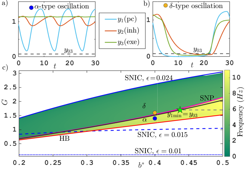
Figure 6: Two-parameter bifurcation diagram for alpha and delta activity in the $(b^{*},G)$ parameter plane. Panel (a,b) show time profile output of typical alpha (panel a, $(b^{*},G)=($(0.4,1.4)$)$, marked by blue circle in panel c) and delta activity (panel b, $(b^{*},G)=($(0.4,1.6)$)$, marked by yellow circle in panel c) for each neuron population at $\epsilon=0.024$. Panel (c) shows the grazing bifurcation of the alpha type periodic orbit for the limiting system ($\epsilon=0$) in black, Folds of periodic orbit (SNP, purple) and Hopf bifurcation (HB, red) are for $\epsilon=0.024$, SNIC bifurcations are shown for $\epsilon=0.024,0.015,0.01$. Horizontal grey dashed line for $b^{*}\in[0.44,0.5]$ at $G=1.7$ was parameter path for continuation to grazing bifurcation, encountered at point labelled by green star. See Table 2 for other parameters.

Mapping alpha and delta oscillations: a two-parameter bifurcation analysis

Following detection of the grazing bifurcation we track its locus in two system parameters, time scale ratio $b^{*}$ between inhibition and excitation, and the ratio $G$ of feedback scale factors between inhibition and excitation. The resulting curve in the $(b^{*},G)$-plane is shown in Figure 6c in black. We combine this curve with the other relevant bifurcations bounding alpha and delta activity:

• The Hopf bifurcation given by $G_{1}=\alpha_{2}b^{*}/(\alpha_{4}+y_{0,1}b^{*}/2)$ in the limit $\epsilon=0$ (see (13)), shown in red in Figure 6c for $\epsilon=0.024$, is the lower bound for alpha activity in $G$. The value $\epsilon=0.024$ is the original value of $\epsilon$ given in Table 2. Visually the Hopf curve for $\epsilon=0.024$ is indistinguishable from its $\epsilon=0$ limit.

• The transition boundary between delta and alpha activity is the grazing curve determined by the algebraic equations (24), (27), shown in black in Figure 6c.

• The upper bound in $G$ for $\delta$ activity is a SNIC bifurcation, determined by the saddle-node of equilibria for the stable small-activity equilibrium, labelled $y_{\mathrm{eq}_{1}}$, and the small-activity saddle $y_{\mathrm{eq}_{2}}$ in Table 3. Table 3 indicates that both equilibria exist for all positive values of $G$ for $\epsilon=0$ and (uniformly in $\epsilon$) positive thresholds $y_{0,1}$ and $y_{0,3}$. Hence, the parameter value $G_{\mathrm{SNIC}}$ for the SNIC bifurcation shown in Figure 2d has the limit $G_{\mathrm{SNIC}}\to 0$ for $\epsilon\to 0$. We included the SNIC bifurcation curve for three values of $\epsilon$ (the original value $0.024$ given in Table 2, $0.015$ and $0.01$) in Figure 6c to visualise the effect of decreasing $\epsilon$. For $(b^{*},G)$ above the SNIC bifurcation curve the activity drops to its small-activity equilibrium.

To demonstrate the quantitative accuracy of the prediction from the singular limit $\epsilon=0$ for the transition between delta and alpha activity, we include shading according to frequency in areas where we find oscillations for the positive value $\epsilon=0.024$ from Table 2. We observe a sharp drop in frequency for increasing $G$ near the singular-limit grazing bifurcation (from yellow to green in Figure 6c). Panels (a) and (b) in Figure 6 show time profiles at representative points in the alpha region ($(b^{*},G)=(0.4,0.14)$, blue circle) and in the delta region ($(b^{*},G)=(0.4,0.16)$, yellow circle). For larger $b^{*}$ a small deviation is noticeable such that the effect of non-zero $\epsilon$ is slightly larger near $b^{*}\approx 0.5$. The pair of folds of periodic orbits which coincides with the frequency drop (see Figure 2(a,d)) is also included for $\epsilon=0.024$ as a purple curve, labelled SNP. It overlaps with the grazing bifurcation bifurcation for $\epsilon=0$ over large parts of the parameter plane.

4 Discussion and further analysis

We have identified the mechanism responsible for the transition between alpha- and delta-type activity in the Jansen-Rit model [15]. The transition between alpha-type oscillations and delta-type oscillations in neural circuits is relevant to applications because alpha frequencies are associated with the promotion of Long-Term Potentiation (LTP), enhancing synaptic strength and facilitating memory formation during active learning, while delta frequencies are associated with Long-Term Depression (LTD), which promotes synaptic weakening and neural plasticity during deep sleep [21]. The combined effects of these processes contribute to of learning via consolidation of memory across the wakefulness and sleep cycles [3, 2]. Therefore, understanding these transitions enhances our knowledge of how neural circuits regulate brain states and may provide insights into disruptions that affect sleep and cognitive functions. In the Jansen-Rit model the transition is not associated with one of the generic codimension-one bifurcations, but it occurs over a small range of parameter values for decreasing excitatory feedback strength $A$ and with little to no hysteresis. In the transition the time profile and the frequency change sharply: oscillations during alpha activity show a shape typical for a single negative feedback loop because of the near-constant support from the excitatory interneurons. Oscillations during delta activity are of relaxation type with long periods of near-zero activity (see Figures 2d,e in Section 2). The feedback strength parameter $A$ affects how neurons respond to incoming signals by scaling the excitable population’s output of firing rates [15].

The results presented in Section 3 show that the singular limit where one assumes that the activation is an all-or-nothing switch reduces the sharp transition in shape and frequency to a grazing bifurcation: when the pyramidal-cell activity “touches” the threshold line for switching off the excitatory interneurons in a quadratic tangency, the excitatory interneuron activity collapses. This causes further drop of pyramidal-cell activity, such that both populations approach near-zero activity. They stay there until the (slower) inhibition activity has dropped sufficiently low to permit recovery of excitatory activity in pyramidal and interneuron populations. (i.e., neuron response to incoming signals acts as binary operation off/on) in Section 3. The singular limit allow us to detect the curve of grazing bifurcation separating the two distinct wave rhythms (i.e., the boundary between two distinct types of periodic orbits) in the two parameter plane $(b^{*},G)$, where $b^{*}$ is the decay rate ratio of inhibitory to excitatory populations and $G$ is the ratio of postsynaptic amplitudes of inhibitory to excitatory populations in non-dimensionalised model (5).

There are several further open questions for the analysis of the singular limit.

Small-threshold analysis of alpha-delta transition and SNIC

Our analysis shows that the limit $\epsilon\to 0$ with fixed thresholds $y_{0,1}$, $y_{0,3}$ does not support delta-type oscillations. In delta-type oscillations all potentials come close to zero such that these oscillations are only possible if there are no stable equilibria at small $y_{1}$, $y_{3}$. However, Figure 6 shows that for all sufficiently small $\epsilon$ there are no parameter values $(b^{*},G)$ for which grazing has happened (so, above the black curve) but no small equilibria exist (below blue solid/dashed/dotted curve called SNIC). If we also consider the thresholds for the excitatory populations as small quantities then delta-type oscillations are possible for small epsilon: as we showed in Section 3.1, if the thresholds are proportional to $\epsilon$ then there are no small equilibria present for small $\epsilon$. A more detailed analysis is needed to find for which asymptotic order of magnitude for the thresholds a saddle-node (and, hence, SNIC) is present for parameters $G$ of order $1$.

The expressions in (24) show that the dependence of the alpha-type periodic orbits on the threshold $y_{0,1}$ is regular, such that a replacing $y_{0,1}$ by zero in (24) will not have a large effect. However, the grazing bifurcation is determined by the minimum of $y_{1}$ reaching $y_{0,3}$, such that for $y_{0,3}\to 0$ the grazing bifurcation will shift. The pyramidal-cell potential $y_{1}$ decays exponentially as long as the inhibition $y_{2}$ is above the equilibrium value of the threshold $y_{3}-y_{0,1}\approx 2\alpha_{2}/G$. As a smaller $b^{*}$ leads to a slow-down in the change of inhibition $y_{2}$, a decrease of $b^{*}$ leads to a longer period of exponential decay for $y_{1}$, so to a smaller minimum of $y_{1}$. Hence, we expect the value of $b^{*}$ for the grazing bifurcation to decrease slowly with $\epsilon$, on the order of $1/|\log\epsilon|$, because of the exponential decay of $y_{1}$ for above threshold inhibition.

Canard explosion of alpha-type orbits at the singular Hopf bifurcation

The Hopf bifurcation, shown in the zoomed-in bifurcation diagram Figure 4 can be studied in the singular limit $\epsilon=0$.

Figure 7: Time profile for alpha-type canard orbit near Hopf bifurcation (labeled HB1, in Fig 4) and activations $\operatorname{S}_{\epsilon/a1}$ for $y_{1}$, and $\operatorname{S}_{\epsilon/a2}$ for $y_{2}$. Parameters: $G=1.49\approx G_{1}=1.48$ (green dashed vertical line in Fig 4 near HB1), $\epsilon=0.001,y_{0,1},y_{0,3}=0.08$ and $y_{02}=0.3$, for others see Table 2. Inset in panel b shows that $y_{2}$ crosses the threshold $y_{\mathrm{3,eq}}-y_{0,1}$ of $y_{1}$.

Figure 7 shows that the periodic orbits in this canard-like explosion are parametrised by the time during which inhibition is switched off (drop of dashed curve in Fiure 7b to zero), which is short for values of the parameter $G$ close to the bifurcation value $G_{1}$. Since the periodic orbits are piecewise exponentials, the asymptotic parameter-amplitude dependence for $G\approx G_{1}$ can be determined explicitly.

Improved limit for slow inhibition

The small thresholds $y_{0,1}$ and $y_{0,3}$ and sharp sigmoid slopes in the activation function $\operatorname{S}_{\epsilon}$ model the fact that excitatory populations have faster internal dynamics. We kept the threshold for the inhibition $y_{0,2}$ non-small, but replaced the activation function of the inhibition $\operatorname{S}_{\epsilon/a_{2}}$ also by an all-or-nothing switch in the limit $\epsilon\to 0$. A more appropriate limit consideration would be to keep a finite-slope sigmoid activation function $\operatorname{S}_{2}(y_{1}-y_{0,2})$ in place for the inhibition and take the small-$\epsilon$ limit only for the excitatory populations. We would still encounter the same dynamical phenomenon for the alpha-delta transition in the limit, namely a grazing bifurcation. However, the limiting periodic orbits of alpha type would no longer be determined by an algebraic system with exponentials, such as (24), but as solutions of a nonlinear ODE over a finite time interval. So, finding the grazing bifurcation would require solving a nonlinear ODE numerically, instead of using the formulas in (24), (27).

Dependence of delta-type oscillations on parameters including non-zero input

Delta-type oscillations in the zero-input case studied have excitation population potentials $y_{1}$ and $y_{3}$ at zero until the inhibition $y_{2}$ drops sufficiently low such that $y_{1}$ and $y_{3}$ can recover and generate a large-amplitude burst (see Figure 2f). The precise time ratios between time spend at zero and bursts depends on time scale ratios such as $b^{*}$, and thresholds. A positive external input $p$ will affect the time profile and frequency of delta-type oscillations, as positive $p$ will prevent $y_{3}$ from staying near zero, resulting in a positive slope at low potential values, as seen in the simulations in [11, 1].

5 Availability of Data

Scripts reproducing the computational data for all figures can be accessed at https://github.com/jansieber/MSTA-alphadelta-anziam24-resources

6 Acknowledgments

KTA gratefully acknowledges the financial support of the Engineering and Physical Sciences Research Council (EPSRC) via grant EP/T017856/1. For the purpose of open access, the corresponding author has applied a ‘Creative Commons Attribution’ (CC BY) licence to any Author Accepted Manuscript version arising from this submission.

Funding statement: Huda Mahdi gratefully acknowledges the Higher Committee for Education Development (HCED), Government of Iraq, for funding her PhD studies.

References

- [1] Ahmadizadeh, S., Karoly, P. J., Nešić, D., Grayden, D. B., Cook, M. J., Soudry, D., and Freestone, D. R. Bifurcation analysis of two coupled Jansen-Rit neural mass models. PloS ONE 13, 3 (2018), e0192842.
- [2] Brudzynski, S. M., Burgdorf, J. S., and Moskal, J. R. From emotional arousal to executive action. Role of the prefrontal cortex. Brain Structure and Function (2024), 1–12.
- [3] Burgdorf, J. S., and Moskal, J. R. A prefrontal cortex alpha/delta switch controls the transition from positive to negative affective states. Discover Mental Health 3, 1 (2023), 19.
- [4] Coletti, A. On Jansen-Rit system modeling epilepsy phenomena. In New Trends in the Applications of Differential Equations in Sciences (Cham, 2023), A. Slavova, Ed., Springer International Publishing, pp. 281–292.
- [5] Da Silva, F. L., Van Rotterdam, A., Barts, P., Van Heusden, E., and Burr, W. Models of neuronal populations: the basic mechanisms of rhythmicity. Progress in brain research 45 (1976), 281–308.
- [6] Dankowicz, H., and Schilder, F. Recipes for Continuation. SIAM, 2013.
- [7] David, O., and Friston, K. J. A neural mass model for MEG/EEG: coupling and neuronal dynamics. NeuroImage 20, 3 (2003), 1743–1755.
- [8] Desroches, M., Krupa, M., and Rodrigues, S. Inflection, canards and excitability threshold in neuronal models. Journal of mathematical biology 67 (2013), 989–1017.
- [9] di Bernardo, M., Budd, C., Champneys, A. R., and Kowalczyk, P. Piecewise-smooth Dynamical Systems: Theory and Applications, vol. 163. Springer Science & Business Media, 2008.
- [10] Ermentrout, B. A guide to xppaut for researchers and students, the society for industrial and applied mathematics. Simulating, analyzing, and animating dynamical systems (2002).
- [11] Forrester, M., Crofts, J. J., Sotiropoulos, S. N., Coombes, S., and O’Dea, R. D. The role of node dynamics in shaping emergent functional connectivity patterns in the brain. Network Neuroscience 4, 2 (2020), 467–483.
- [12] Freeman, W. J. Simulation of chaotic EEG patterns with a dynamic model of the olfactory system. Biological cybernetics 56, 2 (1987), 139–150.
- [13] Grimbert, F., and Faugeras, O. Bifurcation analysis of Jansen’s neural mass model. Neural computation 18, 12 (2006), 3052–3068.
- [14] Guckenheimer, J., and Holmes, P. Nonlinear Oscillations, Dynamical Systems, and Bifurcations of Vector Fields, vol. 42. Springer Science & Business Media, 2013.
- [15] Jansen, B. H., and Rit, V. G. Electroencephalogram and visual evoked potential generation in a mathematical model of coupled cortical columns. Biological cybernetics 73, 4 (1995), 357–366.
- [16] Jansen, B. H., Zouridakis, G., and Brandt, M. E. A neurophysiologically-based mathematical model of flash visual evoked potentials. Biological cybernetics 68, 3 (1993), 275–283.
- [17] Kuznetsov, Y. A. Elements of Applied Bifurcation Theory, third ed., vol. 112 of Applied Mathematical Sciences. Springer-Verlag, New York, 2004.
- [18] Kuznetsov, Y. A., Rinaldi, S., and Gragnani, A. One-parameter bifurcations in planar Filippov systems. International Journal of Bifurcation and Chaos 13, 08 (2003), 2157–2188.
- [19] Lopes da Silva, F., Hoeks, A., Smits, H., and Zetterberg, L. Model of brain rhythmic activity. Kybernetik 15, 1 (1974), 27–37.
- [20] Marten, F., Rodrigues, S., Benjamin, O., Terry, J., and Richardson, M. Onset of poly-spike complexes in a mean-field model of human EEG and its application to absence epilepsy. Philosophical Transactions of the Royal Society A: Mathematical, Physical and Engineering Sciences 367, 1891 (2008), 1145–1161.
- [21] Rashmii, K. S. Long-term potentiation (LTP): a simple yet powerful cellular process in learning and memory. Master’s thesis, Kasturba Medical College, Mangalore, 2021. Publication No. 15.
- [22] Rodrigues, S., Barton, D., Marten, F., Kibuuka, M., Alarcon, G., Richardson, M. P., and Terry, J. R. A method for detecting false bifurcations in dynamical systems: application to neural-field models. Biological cybernetics 102 (2010), 145–154.
- [23] Stefanovski, L., Triebkorn, P., Spiegler, A., Diaz-Cortes, M.-A., Solodkin, A., Jirsa, V., McIntosh, A. R., Ritter, P., and Initiative, A. D. N. Linking molecular pathways and large-scale computational modeling to assess candidate disease mechanisms and pharmacodynamics in alzheimer’s disease. Frontiers in computational neuroscience 13 (2019), 54.
- [24] Touboul, J., and Faugeras, O. Codimension two bifurcations and rythms in neural mass models. arXiv preprint arXiv:0907.2718 (2009).
- [25] van Rotterdam, A., Da Silva, F. L., Van den Ende, J., Viergever, M., and Hermans, A. A model of the spatial-temporal characteristics of the alpha rhythm. Bulletin of mathematical biology 44, 2 (1982), 283–305.
- [26] Wendling, F., Bellanger, J.-J., Bartolomei, F., and Chauvel, P. Relevance of nonlinear lumped-parameter models in the analysis of depth-eeg epileptic signals. Biological cybernetics 83, 4 (2000), 367–378.
- [27] Wilson, H. R., and Cowan, J. D. Excitatory and inhibitory interactions in localized populations of model neurons. Biophysical journal 12, 1 (1972), 1–24.