ACTest: A testing toolkit for analytic continuation methods and codes

Abstract

ACTest is an open-source toolkit developed in the Julia language. Its central goal is to automatically establish analytic continuation testing datasets, which include a large number of spectral functions and the corresponding Green’s functions. These datasets can be used to benchmark various analytic continuation methods and codes. In ACTest, the spectral functions are constructed by a superposition of randomly generated Gaussian, Lorentzian, $\delta$-like, rectangular, and Rise-And-Decay peaks. The spectra can be positive definite or non-positive definite. The corresponding energy grids can be linear or non-linear. ACTest supports both fermionic and bosonic Green’s functions on either imaginary time or Matsubara frequency axes. Artificial noise can be superimposed on the synthetic Green’s functions to simulate realistic Green’s functions obtained by quantum Monte Carlo calculations. ACTest includes a standard testing dataset, namely ACT100. This built-in dataset contains 100 testing cases that cover representative analytic continuation scenarios. Now ACTest is fully integrated with the ACFlow toolkit. It can directly invoke the analytic continuation methods as implemented in the ACFlow toolkit for calculations, analyze calculated results, and evaluate computational efficiency and accuracy. ACTest comprises many examples and detailed documentation. The purpose of this paper is to introduce the major features and usages of the ACTest toolkit. The benchmark results on the ACT100 dataset for the maximum entropy method, which is probably the most popular analytic continuation method, are also presented.

PROGRAM SUMMARY

Program Title: ACTest
CPC Library link to program files: (to be added by Technical Editor)
Developer’s repository link: https://github.com/huangli712/ACTest
Code Ocean capsule: (to be added by Technical Editor)
Licensing provisions (please choose one): GPLv3
Programming language: Julia
Supplementary material:
Journal reference of previous version:*
Does the new version supersede the previous version?:*
Reasons for the new version:*
Summary of revisions:*
Nature of problem (approx. 50-250 words): Analytic continuation is an essential step in quantum many-body computations. It enables the extraction of observable spectral functions from imaginary time or Matsubara frequency Green’s functions. Though numerous methods for analytic continuation were proposed, they have not been systematically and fairly benchmarked due to the lack of testing software and datasets.
Solution method (approx. 50-250 words): At first, a few peaks (features) are generated randomly. Then, they are superimposed to form the spectral function. Finally, the Green’s function is reconstructed from the spectral function via the Laplace transformation. This procedure allows for the generation of lots of spectral functions and corresponding Green’s functions, creating datasets for testing analytic continuation methods and codes.

1 Introduction

In quantum many-body computations, analytic continuation usually plays a vital role. Its objective is to convert Green’s function $G$ from imaginary time ($\tau$) or Matsubara frequency ($i\omega_{n}$) axis to real time ($t$) or real frequency ($\omega$) axis, extracting spectral function $A(\omega)$ for comparison with experimental data [1, 2, 3]. From a mathematical perspective, $G(\tau)$ or $G(i\omega_{n})$ is related to $A(\omega)$ through the well-known Laplace transformation. Given $G(\tau)$ or $G(i\omega_{n})$, analytic continuation calculation is essentially finding the associated $A(\omega)$ that satisfies the Laplace transformation. This is a typical inverse problem. Note that the solution, i.e., $A(\omega)$, is particularly sensitive to numerical fluctuations or noises in the input data, i.e., $G(\tau)$ or $G(i\omega_{n})$. This poses a severe challenge to the analytic continuation methods [4, 5, 6].

Over the past few decades, people have developed many analytic continuation methods, including the Padé approximation [7, 8, 9, 10], maximum entropy method [11, 12, 13, 14], stochastic analytic continuation [15, 16, 17, 18, 19, 20, 21, 22, 23, 24], stochastic optimization method [25, 26], stochastic pole expansion [27, 28], Nevanlinna analytical continuation [29, 30], sparse modeling [31, 32], causal projections [33], Prony fits [34, 35, 36], and machine learning-aided methods [37, 38, 39, 40, 41, 42, 43], to name a few. Unfortunately, nowadays there is no perfect and universal method for solving analytic continuation problems. The existing methods have their own advantages and disadvantages, as well as their scopes of applications. We need a quantitative comparison standard to determine their relative merits. In addition, people have developed several analytic continuation toolkits, such as ACFlow [44], $\Omega$Maxent [45], ana_cont [46], Nevanlnna.jl [47], maxent (in ALPSCore) [48], Nevanlinna (in TRIQS) [49], SOM (in TRIQS) [50, 51], Stoch (in ALF) [52], SmoQyDEAC.jl [53], etc. Are these analytic continuation toolkits reliable? Can their accuracy meet the requirements? These are open questions that need to be addressed.

To answer or solve the aforementioned questions, we would like to introduce an open-source toolkit ACTest in this paper. ACTest can randomly generate a large number of $A(\omega)$, along with the corresponding $G(\tau)$ or $G(i\omega_{n})$. It is worth emphasizing that $G(\tau)$ or $G(i\omega_{n})$ should be supplemented with artificial noises to mimic input data from realistic quantum many-body calculations. The synthetic $A(\omega)$ and $G(\tau)$ [or $G(i\omega_{n})$] can be used to benchmark the existing or newly developed analytic continuation methods, examining their computational accuracies and efficiencies. The ACTest toolkit comes with a standard dataset containing 100 spectral functions, known as ACT100. This built-in dataset can be used to assess the merits of different analytic continuation methods in a relatively fair, reproducible, and quantitative manner. People can also employ the ACTest toolkit to create large datasets, which can serve as training and testing datasets for machine learning-aided methods [37, 38, 39, 40, 41, 42, 43]. Currently, the ACTest toolkit has been integrated with the ACFlow toolkit [44]. Thus, it allows direct calls of various methods as implemented in the ACFlow toolkit for analytic continuation calculations.

The rest of this paper is organized as follows. In Section 2, the technical details inside the ACTest toolkit are overviewed. Section 3 is the major part of this paper. It elaborates on the basic usages of the ACTest toolkit, including installation, scripts, input files, output files, and control parameters. In Section 4, an illustrative example is presented. It shows how to generate spectral functions and Green’s functions, how to invoke the maximum entropy method in the ACFlow toolkit for massive analytic continuation calculations, and how to visualize the benchmark results, by using the ACTest toolkit. Finally, a brief summary is given in Section 5.

2 Overview

2.1 Major features

The current version of the ACTest toolkit is v1.0. Its major features are as follows:

• ACTest can randomly generate any number of $A(\omega)$, as well as corresponding $G(\tau)$ or $G(i\omega_{n})$.

• ACTest employs one or more parameterized Gaussian, Lorentzian, $\delta$-like, rectangular, and Rise-And-Decay peaks to assemble $A(\omega)$. $A(\omega)$ can be either positive definite for fermionic Green’s functions, or non-positive definite for bosonic Green’s functions and matrix-valued Green’s functions. The frequency grid, i.e., $\omega$, can be either linear or non-linear (such as tangent, Lorentzian, and half-Lorentzian grids).

• ACTest supports fermionic, bosonic, and symmetric bosonic kernels to generate Green’s functions on either imaginary time or Matsubara frequency axes. It supports artificial noise, and the noise level is adjustable.

• ACTest includes a built-in testing dataset, ACT100, which can serve as a relatively fair standard for examining different analytic continuation methods and codes.

• ACTest is already interfaced with ACFlow, which is a full-fledged and open-source analytic continuation toolkit [44]. ACTest can access various analytic continuation methods in the ACFlow toolkit, launch them to perform analytic continuation calculations, and provide benchmark reports on their accuracy and efficiency. ACTest also provides a plotting script, that can be used to visualize and compare the true and reconstructed spectral functions.

• ACTest is an open-source software developed in Julia language. It is quite easy to be extended to implement new features or support the other analytic continuation codes, such as Nevanlinna.jl [47] and SmoQyDEAC.jl [53]. Furthermore, ACTest offers extensive documentation and examples, making it user-friendly.

In the following text, we will elaborate on the technical details inside ACTest.

2.2 Grids for Green’s functions

As mentioned before, Green’s functions in quantum many-body physics are usually defined on imaginary time or Matsubara frequency axes. Imaginary time Green’s functions $G(\tau)$ and Matsubara Green’s functions $G(i\omega_{n})$ are related via Fourier transformation [1, 2, 3]:

$$G(\tau)=\frac{1}{\beta}\sum_{n}e^{i\omega_{n}\tau}G(i\omega_{n}),$$ (1)

and

$$G(i\omega_{n})=\int^{\beta}_{0}d\tau\ e^{-i\omega_{n}\tau}G(\tau),$$ (2)

where $\beta$ denotes inverse temperature ($\beta\equiv 1/T$). The grids for Green’s functions are linear. Specifically, $\tau_{i}=i\beta/N_{\tau}$, where $N_{\tau}$ denotes number of time slices and $i\in[0,N_{\tau}]$. $\omega_{n}=(2n+1)\pi/\beta$ for fermions and $2n\pi/\beta$ for bosons, where $n\in[0,N]$ and $N$ means number of Matsubara frequency points.

2.3 Meshes for spectral functions

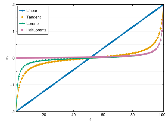
Figure 1: The four frequency meshes supported in ACTest: linear, tangent, Lorentzian, and half-Lorentzian meshes. The parameters for these meshes are $\omega_{\text{max}}=-\omega_{\text{min}}=2.0$ and $N_{\omega}=101$.

The spectral function $A(\omega)$ is defined on the real frequency axis. The frequency range for $\omega$ is restricted in $[\omega_{\text{min}},\omega_{\text{max}}]$, where $N_{\omega}$ represents the number of mesh points, $\omega_{\text{min}}$ and $\omega_{\text{max}}$ denote the left and right boundaries of the mesh, respectively. Currently, the ACTest toolkit supports four types of meshes: linear, tangent, Lorentzian, and half-Lorentzian meshes. The latter three meshes are non-linear, with the highest grid density near $\omega=0$. As its name suggests, the half-Lorentzian mesh is only suitable for cases where $\omega\geq 0$. Figure 1 illustrates typical examples of the four meshes.

2.4 Peaks

In the ACTest toolkit, the spectral function $A(\omega)$ is treated as a superposition of some peaks (i.e. features). That is to say:

$$A(\omega)=\sum^{N_{p}}_{i=1}p_{i}(\omega),$$ (3)

where $N_{p}$ is the number of peaks, $p(\omega)$ is the peak generation function. Now ACTest supports the following types of peaks:

• Gaussian peak

  $$p(\omega)=A\exp{\left[-\frac{(\omega-\epsilon)^{2}}{2\Gamma^{2}}\right]}$$ (4)

• Lorentzian peak

  $$p(\omega)=\frac{A}{\pi}\frac{\Gamma}{(\omega-\epsilon)^{2}+\Gamma^{2}}$$ (5)

• $\delta$-like peak

  $$p(\omega)=A\exp{\left[-\frac{(\omega-\epsilon)^{2}}{2\gamma^{2}}\right]},~{}\text{where}~{}\gamma=0.01$$ (6)

• Rectangular peak

  $$p(\omega)=\begin{cases}h,\quad\text{if}~{}\omega\in[c-w/2,c+w/2],\\ 0,\quad\text{else}.\\ \end{cases}$$ (7)

• Rise-And-Decay peak

  $$p(\omega)=h\exp{(-|\omega-c|^{\gamma})}$$ (8)

Here we just use a narrow Gaussian peak to mimic the $\delta$-like peak. In Eq. (4)-(8), $\mathcal{C}=\{A,~{}\Gamma,~{}\epsilon,~{}h,~{}c,~{}w,~{}\gamma\}$ is a collection for essential parameters. The ACTest toolkit will randomize $\mathcal{C}$ and use it to parameterize the peaks.

2.5 Kernels

Just as stated above, the spectral function and the imaginary time or Matsubara Green’s function are related with each other by the Laplace transformation:

$$G(x)=\int d\omega~{}K(x,\omega)A(\omega).$$ (9)

Here $K(x,\omega)$ is the so-called kernel function [27]. It plays a key role in this equation. In this section, we would like to introduce the kernels that have been implemented in ACTest.

2.5.1 Fermionic kernels

For fermionic Green’s function, we have

$$G(\tau)=\int^{+\infty}_{-\infty}d\omega\frac{e^{-\tau\omega}}{1+e^{-\beta\omega}}A(\omega),$$ (10)

and

$$G(i\omega_{n})=\int^{+\infty}_{-\infty}d\omega\frac{1}{i\omega_{n}-\omega}A(\omega).$$ (11)

The kernels are defined as

$$K(\tau,\omega)=\frac{e^{-\tau\omega}}{1+e^{-\beta\omega}},$$ (12)

and

$$K(\omega_{n},\omega)=\frac{1}{i\omega_{n}-\omega}.$$ (13)

For fermionic systems, $A(\omega)$ is defined on $(-\infty,\infty)$. It is causal, i.e., $A(\omega)\geq 0$.

2.5.2 Bosonic kernels

For bosonic system, the spectral function obeys the following constraint:

$$\text{sign}(\omega)A(\omega)\geq 0.$$ (14)

It is quite convenient to introduce a new variable $\tilde{A}(\omega)$:

$$\tilde{A}(\omega)=\frac{A(\omega)}{\omega}.$$ (15)

Clearly, $\tilde{A}(\omega)\geq 0$. It means that $\tilde{A}(\omega)$ is positive definite. So, we have

$$G(\tau)=\int^{+\infty}_{-\infty}d\omega\frac{e^{-\tau\omega}}{1-e^{-\beta\omega}}A(\omega)=\int^{+\infty}_{-\infty}d\omega\frac{\omega e^{-\tau\omega}}{1-e^{-\beta\omega}}\tilde{A}(\omega),$$ (16)

and

$$G_{B}(i\omega_{n})=\int^{+\infty}_{-\infty}d\omega\frac{1}{i\omega_{n}-\omega}A(\omega)=\int^{+\infty}_{-\infty}d\omega\frac{\omega}{i\omega_{n}-\omega}\tilde{A}(\omega).$$ (17)

The corresponding kernels read:

$$K(\tau,\omega)=\frac{\omega e^{-\tau\omega}}{1-e^{-\beta\omega}},$$ (18)

and

$$K(\omega_{n},\omega)=\frac{\omega}{i\omega_{n}-\omega}.$$ (19)

Especially,

$$K(\tau,\omega=0)\equiv\frac{1}{\beta},$$ (20)

and

$$K(\omega_{n}=0,\omega=0)\equiv-1.$$ (21)

2.5.3 Symmetric bosonic kernels

This is a special case for the bosonic Green’s function with Hermitian bosonic operators. Here, the spectral function $A(\omega)$ is an odd function. Let us introduce $\tilde{A}(\omega)=A(\omega)/\omega$ again. Since $\tilde{A}(\omega)$ is an even function, we can restrict it in $(0,\infty)$. Now we have

$$G(\tau)=\int^{\infty}_{0}d\omega\frac{\omega[e^{-\tau\omega}+e^{-(\beta-\tau)\omega}]}{1-e^{-\beta\omega}}\tilde{A}(\omega),$$ (22)

and

$$G(i\omega_{n})=\int^{\infty}_{0}d\omega\frac{-2\omega^{2}}{\omega_{n}^{2}+\omega^{2}}\tilde{A}(\omega).$$ (23)

The corresponding kernel functions read:

$$K(\tau,\omega)=\frac{\omega[e^{-\tau\omega}+e^{-(\beta-\tau)\omega}]}{1-e^{-\beta\omega}},$$ (24)

and

$$K(\omega_{n},\omega)=\frac{-2\omega^{2}}{\omega_{n}^{2}+\omega^{2}}.$$ (25)

There are two special cases:

$$K(\tau,\omega=0)=\frac{2}{\beta},$$ (26)

and

$$K(\omega_{n}=0,\omega=0)=-2.$$ (27)

2.6 Artificial noise

Assuming that we already construct the spectral function $A(\omega)$, it is then straightforward to calculate $G(\tau)$ or $G(i\omega_{n})$ via Eqs. (10)-(27). At this point, the synthetic Green’s function $G$ is exact, containing no numerical noise. We name it $G_{\text{exact}}$. However, the Green’s functions obtained from quantum many-body calculations are often noisy [4, 5, 6]. This is especially the case in finite-temperature quantum Monte Carlo simulations, where numerical noise is inevitable. To make things worse, when the fermionic sign problem is severe, the noise correspondingly increases. To simulate this scenario, the ACTest toolkit can introduce artificial noise into the synthetic Green’s function as follows [33]:

$$G_{\text{noisy}}=G_{\text{exact}}[1+\delta\mathcal{N}_{C}(0,1)]$$ (28)

where $\mathcal{N}_{C}(0,1)$ represents complex-valued Gaussian noise with zero mean and unit variance, and the parameter $\delta$ is used to control the noise level ($0\leq\delta\leq 1$).

2.7 Built-in testing dataset

The ACTest toolkit operates in two modes. On one hand, ACTest can randomly generate a large number of spectral functions and Green’s functions. People can use them to train or examine machine learning models for solving analytic continuation problems. On the other hand, ACTest includes a “standard” testing dataset. This dataset comprises 100 representative tests, 50 for fermionic systems and 50 for bosonic systems. Hence we name it the ACT100 dataset. In this dataset, the spectral functions are constructed with predefined parameters (it means that all the peaks and features in these spectra are certain), so they are reproducible. Note that users can only change the grids and the noise levels of the synthetic Green’s functions. The basic configurations regarding the fermionic subset of the ACT100 dataset are shown in Table 1. As for the bosonic subset, the basic configurations are identical. The only difference is the use of bosonic kernels to generate the Green’s functions. Four typical spectral functions in the ACT100 dataset are illustrated in Figure 2.

Table 1: Basic configurations about the fermionic subset in the ACT100 dataset. Clearly, the fermionic subset is classified into three parts. Both the first and the second parts are for diagonal Green’s functions, where $A(\omega)$ is positive. Their spectra are continuum and discrete, respectively. The third part is for off-diagonal Green’s functions, where $A(\omega)$ is non-positive definite and continuum. The configurations for the bosonic subset are the same. It is also classified into three parts according to positive definiteness of $\tilde{A}(\omega)$ [$\equiv A(\omega)/\omega$]. Full parameters for constructing these spectra are defined in actest/src/dataset.jl.

System	Spectrum’s type	Peak’s type	Number of peaks	Number of spectra / tests
Fermionic	Continuum spectrum,	Gaussian	1	3
	$A(\omega)\geq 0$		2	7
			3	10
Fermionic	Discrete spectrum,	Gaussian	1	5
	$A(\omega)\geq 0$		2	5
			3	2
			4	3
			5	3
			6	2
Fermionic	Continuum spectrum,	Rise-And-Decay	1	1
	$A(\omega)$ is non-positive definite		2	5
			3	2
			4	1
			5	1

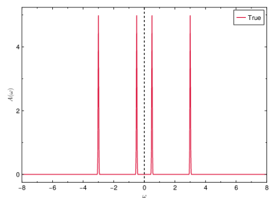
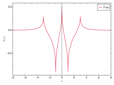
Figure 2: Four representative spectra in the ACT100 dataset. The vertical dashed lines denote the Fermi level. The raw data and figures are generated by the actest/util/acstd.jl and actest/util/acplot.jl scripts, respectively. See Section 3.2 for more details.

The ACT100 dataset can be utilized to assess the accuracy of various analytic continuation methods. The question is how to measure the accuracy. Supposed that the true spectral function and the calculated spectral function are $A_{\text{true}}(\omega)$ and $A_{\text{calc}}(\omega)$, respectively, their difference can be calculated by the following expression [36]:

$$\text{Err}(A_{\text{true}},A_{\text{calc}})=\int^{\omega_{\text{max}}}_{\omega_{\text{min}}}d\omega~{}\Big{|}A_{\text{true}}(\omega)-A_{\text{calc}}(\omega)\Big{|}~{}\Big{/}~{}\int^{\omega_{\text{max}}}_{\omega_{\text{min}}}d\omega~{}|A_{\text{true}}(\omega)|.$$ (29)

It is evident that the smaller the value of Err($A_{\text{true}},A_{\text{calc}}$), the better. Thus, the accuracy of an analytic continuation method can be evaluated by:

$$f=\sum^{N_{\text{test}}}_{i=1}\theta\left[1-\text{Err}\left(A^{i}_{\text{true}},A^{i}_{\text{calc}}\right)\right]\left[1-\text{Err}\left(A^{i}_{\text{true}},A^{i}_{\text{calc}}\right)\right].$$ (30)

Here, $N_{\text{test}}$ is the number of tests, $i$ is the index, $\theta(x)$ is the Heaviside step function. It is obvious that $\text{max}(f)=N_{\text{test}}$ and $\text{min}(f)=0$.

2.8 Interface to analytic continuation toolkits

The ACTest toolkit is not only capable of generating testing datasets, but also of invoking external programs for analytic continuation calculations. Currently, it is integrated with the ACFlow toolkit via the actest/util/acflow.jl script. ACFlow is an open-source toolkit written in Julia [44]. It supports a variety of highly optimized analytic continuation methods, including the maximum entropy method [11, 12, 13, 14], barycentric rational function approximation [54, 55], Nevanlinna analytical continuation [29, 30], stochastic analytic continuation (both the Beach’s algorithm [15] and Sanvik’s algorithm [18, 19, 16, 17] are supported), stochastic optimization method [25, 26], and stochastic pole expansion [27, 28], etc. The ACTest toolkit is designed in a modular fashion, making it not very difficult to interface with other analytic continuation tools.

3 Basic usage

3.1 Installation

3.1.1 Prerequisites

We chose the Julia language to develop the ACTest toolkit. Julia is an interpreted language. Hence, to run the ACTest toolkit, the latest version of the Julia interpreter must be installed on the target system. Actually, Julia’s version number should not be less than 1.6. The core features of the ACTest toolkit rely only on Julia’s standard library. However, if one needs to invoke the ACFlow toolkit for analytic continuation calculations, the toolkit must be available in the system. As for how to install and configure the ACFlow toolkit, please refer to the relevant paper [44]. Additionally, if one wants to use the built-in script of ACTest to visualize the calculated results (i.e., the spectral functions), support from the CairoMakie.jl package is necessary. CairoMakie.jl is a 2D plotting program developed in Julia. It can be installed via Julia’s package manager:

    julia> ]
    (@v1.11) pkg> add CairoMakie

3.1.2 Main program

The official repository of the ACTest toolkit is hosted on github. Its URL is as follows:

    https://github.com/huangli712/ACTest

Since the ACTest toolkit has not yet been registered as a regular Julia package, please type the following commands in Julia’s REPL to install it:

    julia> using Pkg
    julia> Pkg.add("https://github.com/huangli712/ACTest")

If this method fails due to an unstable network connection, an offline method should be adopted. First of all, please download the compressed package for the ACTest toolkit from github. Usually it is called actest.tar.gz or actest.zip. Second, please copy it to your favorite directory (such as /home/your_home), and then enter the following command in the terminal to decompress it:

    $ tar xvfz actest.tar.gz

or

    $ unzip actest.zip

Finally, we just assume that the ACTest toolkit is placed in the directory:

    /home/your_home/actest

Now we have to manually insert the following codes at the beginning of all ACTest’s scripts (see Section 3.2):

    # Add the ACTest package to the Julia load path
    push!(LOAD_PATH, "/home/your_home/actest/src")

These modifications just ensure that the Julia interpreter can find and import the ACTest toolkit correctly. Now it should work as expected.

3.1.3 Documentation

The ACTest toolkit ships with detailed documentation, including the user’s manual and application programming interface. They are developed with the Markdown language and the Documenter.jl package. So, please make sure that the latest version of the Documenter.jl package is ready (see https://github.com/JuliaDocs/Documenter.jl for more details). If everything is OK, users can generate the documentation by themselves. Please enter the following commands in the terminal:

    $ pwd
    /home/your_home/actest
    $ cd docs
    $ julia make.jl

After a few seconds, the documentation is built and saved in the actest/docs/build directory. The entry of the documentation is actest/docs/build/index.html. You can open it with any web browser.

3.2 Scripts

The ACTest toolkit provides four Julia scripts. They are located in the actest/util directory. Here are brief descriptions for these scripts:

• acgen.jl

  This is the core script of the ACTest toolkit. It is able to randomly generate any number of spectral functions and corresponding Green’s functions according to the user’s settings.

• acstd.jl

  It is similar to acgen.jl. But its task is to generate the ACT100 dataset, which includes 100 predefined spectral functions and corresponding Green’s functions.

• acflow.jl

  This script provides a bridge between the ACTest toolkit and the ACFlow toolkit [44]. At first, it will parse outputs from the acgen.jl or acstd.jl script to get the synthetic Green’s functions. Next, these Green’s functions are fed into the ACFlow toolkit, which will perform analytic continuation calculations and return the calculated spectral functions. Finally, acflow.jl script will compare the calculated spectral functions with the true solutions, and produce benchmark reports. This script needs support of the ACFlow toolkit.

• acplot.jl

  It is able to read $A_{\text{calc}}(\omega)$ and $A_{\text{true}}(\omega)$, and plot them in the same figure for comparison. It adopts the PDF format to output the figure. This script requires support of the CairoMakie.jl package.

Please execute the above scripts using the following command:

    $ actest/util/script_name act.toml

Here, act.toml is the configuration file. It is a standard TOML file, primarily used for storing user’s settings (i.e., control parameters). The technical details of the act.toml file will be introduced in the following text.

3.3 Inputs

The scripts in the ACTest toolkit require only one input file, which is act.toml. Below is a typical act.toml file with some omissions. In this act.toml, text following the “#” symbol is considered as a comment. It contains two sections: [Test] and [Solver]. The [Test] section is mandatory, which controls generation of spectral functions and corresponding Green’s functions. We would like to explain the relevant control parameters in the following text. The [Solver] section is optional. Now it is used to configure the analytic continuation methods as implemented in the ACFlow toolkit [44]. Only the acflow.jl script needs to read the [Solver] section. It will transfer these parameters to the ACFlow toolkit to customize the successive analytic continuation calculations. For possible parameters within the [Solver] section, please refer to the documentation of the ACFlow toolkit [44].

⬇

#

# Test: A01

#

# 1. Execute ../../util/acgen.jl act.toml.

# 2. Change solver = "MaxEnt" and modify the [Solver] section accordingly.

# 3. Execute ../../util/acflow.jl act.toml.

# 4. Execute ../../util/acplot.jl act.toml.

#

[Test]

solver = "MaxEnt"

...

[Solver]

method = "chi2kink"

...

3.4 Outputs

Both acgen.jl and acstd.jl scripts generate image.data.i and green.data.i files. The image.data.i file stores the exact spectral function, i.e., $A_{\text{true}}(\omega)$. The green.data.i file stores the imaginary time Green’s function $G(\tau)$ or the Matsubara Green’s function $G(i\omega_{n})$. The suffix $i$ in filename denotes index for tests. It starts from 1. The acflow.jl script will output quite a few files. The most important one is Aout.data.i. For other possible output files, please refer to the documentation of the ACFlow toolkit [44]. The Aout.data.i file stores the calculated spectral function, i.e., $A_{\text{calc}}(\omega)$. The suffix $i$ in filename also represents index for tests. The aforementioned files are column-based plain texts. They can be opened by any text editor. Their file formats are summarized in Table 2. As for the acplot.jl script, it will generate image.i.pdf files, which are image files for $A_{\text{true}}(\omega)$ and $A_{\text{calc}}(\omega)$. Actually, the data from the image.data.i and Aout.data.i files are used to generate the image.i.pdf file.

Table 2: File formats for selected files generated by the ACTest toolkit. Here, Var[$G$] means error bar for $G$. Re$G$ and Im$G$ mean real and imaginary parts of $G$, respectively.

Filename	Column 1	Column 2	Column 3	Column 4	Column 5	Number of lines
image.data.i	$\omega$	$A_{\text{true}}(\omega)$	-	-	-	$N_{\omega}$
green.data.i	$\tau$	$G(\tau)$	$\text{Var}[G(\tau)]$	-	-	$N_{\tau}$
green.data.i	$i\omega_{n}$	$\text{Re}G(i\omega_{n})$	$\text{Im}G(i\omega_{n})$	$\text{Var}[\text{Re}G(i\omega_{n})]$	$\text{Var}[\text{Im}G(i\omega_{n})]$	$N$
Aout.data.i	$\omega$	$A_{\text{calc}}(\omega)$	-	-	-	$N_{\omega}$

3.5 Parameters

In this subsection, we will provide brief explanations of the control parameters of the ACTest toolkit. The detailed descriptions for these parameters are available in the user’s manual. As mentioned before, the act.toml file contains two sections: [Test] and [Solver]. The parameters described here are specific to the [Test] section. They are primarily used for setting generation rules for the spectral functions and Green’s functions. However, the parameters within the [Solver] section will be transferred to the ACFlow toolkit for configuring the analytic continuation methods. They will be explained in the documentation of the ACFlow toolkit [44].

• solver

  Specify analytic continuation solver. Possible values include “MaxEnt”, “BarRat”, “NevanAC”, “StochAC”, “StochSK”, “StochOM”, and “StochPX”. They are the analytic continuation methods supported by the ACFlow toolkit. This parameter is only relevant for the acflow.jl and acplot.jl scripts.

• ptype

  Specify type of peaks. Possible values include “gauss”, “lorentz”, “delta”, “rectangle”, and “risedecay”. They are corresponding to the Gaussian, Lorentzian, $\delta$-like, rectangular, and Rise-And-Decay peaks, respectively. This parameter is only relevant for the acgen.jl script. See Section 2.4 for more details.

• ktype

  Specify kernel function. Possible values include “fermi”, “boson”, and “bsymm”. They are corresponding to the fermionic, bosonic, and symmetric bosonic kernels, respectively. See Section 2.5 for more details.

• grid

  Specify grid for the Green’s functions. Possible values include “ftime”, “btime”, “ffreq”, and “bfreq”. Here, the characters “f” and “b” mean fermionic and bosonic, respectively. The strings “time” and “freq” mean imaginary time and Matsubara frequency axes, respectively. See Section 2.2 for more details.

• mesh

  Specify mesh for the spectral function. Possible values are “linear”, “tangent”, “lorentz”, and “halflorentz”. They are corresponding to the linear, tangent, Lorentzian, and half-Lorentzian meshes, respectively. See Section 2.3 for more details.

• ngrid

  Number of imaginary time or Matsubara frequency points for the Green’s function. It denotes $N_{\tau}$ or $N$. See Section 2.2 for more details.

• nmesh

  Number of mesh points for the spectral function. It is $N_{\omega}$. See Section 2.3 for more details.

• ntest

  How many spectral functions and corresponding Green’s functions are generated by the ACTest toolkit? It is the size of the testing dataset for analytic continuation methods or codes.

• wmax

  Right boundary of the real frequency mesh ($\omega_{\text{max}}$). See Section 2.3 for more details.

• wmin

  Left boundary of the real frequency mesh ($\omega_{\text{min}}$). See Section 2.3 for more details.

• pmax

  Right boundary of features in the spectrum. It is used to restrict the centers of Gaussian and Lorentzian peaks. $\texttt{wmin}<\texttt{pmin}<\texttt{pmax}<\texttt{wmax}$. See Section 2.4 for more details.

• pmin

  Left boundary of features in the spectrum. It is used to restrict the centers of Gaussian and Lorentzian peaks. $\texttt{wmin}<\texttt{pmin}<\texttt{pmax}<\texttt{wmax}$. See Section 2.4 for more details.

• beta

  Inverse temperature of the system $\beta$ ($\equiv 1/T$). It is used to define the imaginary time or Matsubara frequency grids for Green’s functions. See Section 2.2 for more details.

• noise

  The noise level, i.e., the $\delta$ parameter seen in Eq. (28). See Section 2.6 for more details.

• offdiag

  Specify whether the spectral function is positive definite or not. If offdiag is true, it implies that the spectral function is not positive definite and the ACTest toolkit will generate off-diagonal Green’s function.

• lpeak

  It is an integer array that sets the number of peaks (features) that the synthetic spectral function may contain. For example: lpeak = [1,2,3,4,5], then the ACTest toolkit can generate spectral functions with the number of peaks ranging from 1 to 5. This parameter is only relevant for the acgen.jl script.

4 Examples

In the actest/tests directory, there are seven typical test cases. Users can modify them to meet their requirements. This section will use an independent example to demonstrate the basic usage of the ACTest toolkit.

4.1 Generating spectra and correlators

Now let us test the performance of the maximum entropy method [11, 12, 13, 14] in the ACFlow toolkit [44]. We just consider four typical scenarios: (1) Fermionic Green’s functions, $A(\omega)>0$; (2) Fermionic Green’s functions, $A(\omega)$ is non-positive definite; (3) Bosonic Green’s functions, $A(\omega)>0$; (4) Bosonic Green’s functions, $A(\omega)$ is non-positive definite. For each scenario, we apply the ACTest toolkit to randomly generate 100 spectral functions and corresponding Green’s functions. The spectral functions are continuum. They are constructed with Gaussian peaks. The number of possible peaks in each $A(\omega)$ ranges from 1 to 6. The synthetic Green’s functions are on the Matsubara frequency axis. The number of Matsubara frequency points is 10. The noise level is $10^{-6}$. The act.toml file for scenario (3) is shown below.

⬇

[Test]

solver = "MaxEnt" # Analytic continuation solver in the ACFlow toolkit

ptype = "gauss" # Type of peaks

ktype = "boson" # Type of kernels

grid = "bfreq" # Type of grids

mesh = "linear" # Type of meshes

ngrid = 10 # Number of grid points

nmesh = 801 # Number of mesh points

ntest = 100 # Number of tests

wmax = 8.0 # Right boundary of frequency mesh

wmin = -8.0 # Left boundary of frequency mesh

pmax = 4.0 # Right boundary of peaks

pmin = -4.0 # Left boundary of peaks

beta = 20.0 # Inverse temperature

noise = 1.0e-6 # Noise level

offdiag = false # Whether the spectrum is positive

lpeak = [1,2,3,4,5,6] # Possible number of peaks

Once the act.toml file is prepared, the following command should be executed in the terminal:

    $ actest/util/acgen.jl act.toml

Then, the ACTest toolkit will generate the required data in the present directory. Now there are 100 image.data.i and green.data.i files, where $i$ ranges from 1 to 100. These correspond to $A(\omega)$ and $G(i\omega_{n})$ for bosonic systems. We can further verify the data to make sure $A(\omega)>0$. Finally, we have to copy the act.toml file to another directory, change the ktype, grid, and offdiag parameters in it, and then execute the above command again to generate testing datasets for the other scenarios.

4.2 Analytic continuation simulations

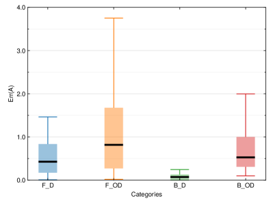
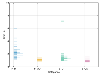
Figure 3: Tests of the maximum entropy method as implemented in the ACFlow package [44]. The tests are classified as four categories (scenarios): (1) F_D, (2) F_OD, (3) B_D, and (4) B_OD. Here, “F” means fermionic systems and “B” means bosonic systems. “D” means diagonal Green’s functions [$A(\omega)>0$] and “OD” means off-diagonal Green’s functions [$A(\omega)$ is non-positive definite]. Each category contains 100 tests. In this figure, the information contained in the summary.data file is visualized. (Left) Box-and-whisker plot for error statistics. Err(A) is calculated by using Eq. (29). The black solid segments denote the median values. (Right) Histogram plot for duration times consumed in the tests.

Next, we have to add a [Solver] section in the act.toml file to setup the control parameters for the MaxEnt analytic continuation solver (which implements the maximum entropy method) in the ACFlow toolkit [44]. The spirit of the maximum entropy entropy is to figure out the optimal $A$, that minimizes the following functional [11]:

$$Q[A]=\frac{1}{2}\chi^{2}[A]-\alpha S[A].$$ (31)

Here, $\chi^{2}$ is the so-called goodness-of-fit functional, which measures the distance between the reconstructed Green’s function and the original Green’s function. $S$ is the entropic term. Usually the Shannon-Jaynes entropy is used. $\alpha$ is a hyperparameter. In this example, we adopt the chi2kink algorithm [45] to determine the optimized $\alpha$ parameters. The list of the $\alpha$ parameters contains 10 elements. The initial value of $\alpha$ is $\alpha_{1}=10^{12}$, and the ratio between two consecutive $\alpha$ parameters ($\alpha_{i}/\alpha_{i+1}$) is 10. The complete [Solver] section is shown as follows:

⬇

[Solver]

method = "chi2kink" # Method to optimize the \alpha parameter

stype = "sj" # Typer of the entropic term

nalph = 12 # Number of \alpha parameter

alpha = 1e12 # Initial value of \alpha

ratio = 10.0 # Ratio between two successive \alpha parameters

blur = -1.0 # Whether we should broaden the kernel

Please execute the following command in the terminal:

    $ actest/util/acflow.jl act.toml

It will launch the ACFlow toolkit [44] to perform analytic continuation calculations and generate a lot of output files. In addition to the Aout.data.i file, perhaps the most important file is summary.data. It records the error, status (pass or fail), and duration time for each test. So, we visualize the summary.data file in Figure 3. It is evident that the errors for the analytic continuations of non-diagonal Green’s functions [i.e., scenarios (2) and (4)] are slightly larger than those of diagonal Green’s functions [i.e., scenarios (1) and (3)]. Furthermore, scenarios (2) and (4) consume much less time to solve the problems. Surprisingly, we found that the pass rates for scenarios (1) and (3) are approximately 80%, while those for scenarios (2) and (4) are close to 100%. If we further change the computational configurations (such as increasing the size of the dataset, altering the noise level or changing the type of peaks), and then repeat the aforementioned tests, the final conclusions could be similar.

4.3 Visualizations

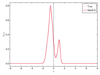
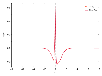
Figure 4: Selected analytic continuation results for Matsubara Green’s functions (fermionic systems). (Left) Spectra for diagonal Green’s function. (Right) Spectra for off-diagonal Green’s function. The exact spectra are generated randomly by the ACTest toolkit. The vertical dashed lines denote the Fermi level.

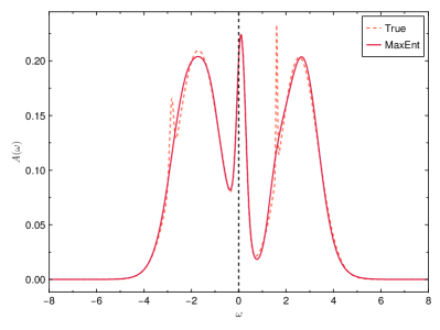
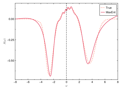
Figure 5: Selected analytic continuation results for Matsubara Green’s functions (bosonic systems). (Left) Spectra for diagonal Green’s function. (Right) Spectra for off-diagonal Green’s function. The exact spectra are generated randomly by the ACTest toolkit. The vertical dashed lines denote the Fermi level.

Finally, we can utilize the acplot.jl script to generate figures for the spectral functions. To achieve that effect, please execute the following command in the terminal:

    $ actest/util/acplot.jl act.toml

These figures are in standard PDF format. They are used to analyze the differences between the true spectral functions $A_{\text{true}}(\omega)$ and the calculated spectral functions $A_{\text{calc}}(\omega)$. Figures 4 and  5 illustrate the spectral functions of typical fermionic systems and bosonic systems, respectively. As can be seen from the figures, aside from some very sharp peaks, the calculated spectral functions agree quite well with the true ones.

5 Concluding remarks

In this paper, we introduce the open-source toolkit ACTest, which is designed to generate a large set of spectral functions and corresponding Green’s functions for benchmarking analytic continuation algorithms and codes. The toolkit provides a flexible framework to support various grids, meshes, peaks, and kernels. It also supports artificial noise to mimic the realistic Green’s functions from quantum many-body computations. The most important feature of ACTest is that it includes a built-in testing dataset, ACT100, which can be used to assess the existing analytic continuation methods in a reproducible and quantitative manner. Now ACTest is interoperable with the ACFlow toolkit, facilitating applications of various analytic continuation methods.

The ACTest toolkit holds promise for significant contributions to the field of solving analytic continuation problems. First of all, it can be used as a validation tool to examine the newly developed analytic continuation methods. Second, if we don’t know what kind of analytic continuation problems the present method can deal with, we can turn to ACTest. It will help us to uncover the pros and cons of the present method. Finally, the ACTest toolkit can be used to generate training data for machine learning models. In the future, we would like to extend the ACTest toolkit to support more complex spectral functions and more analytic continuation tools.

Declaration of competing interest

The author declares that he has no known competing financial interests or personal relationships that could have appeared to influence the work reported in this paper.

Data availability

The data that support the findings of this study will be made available upon reasonable requests to the corresponding author.

Acknowledgement

This work is supported by the National Natural Science Foundation of China (under Grants No. 11874329 and No. 11934020).

References

- [1] J. W. Negele, H. Orland, Quantum Many-Particle Systems, Perseus Books, 1998. doi:10.1201/9780429497926.
- [2] P. Coleman, Introduction to Many-Body Physics, Cambridge University Press, 2016. doi:10.1017/CBO9781139020916.
-
[3]
A. Georges, G. Kotliar, W. Krauth, M. J. Rozenberg,
Dynamical
mean-field theory of strongly correlated fermion systems and the limit of
infinite dimensions, Rev. Mod. Phys. 68 (1996) 13–125.
doi:10.1103/RevModPhys.68.13.
URL https://link.aps.org/doi/10.1103/RevModPhys.68.13 -
[4]
M. Asakawa, Y. Nakahara, T. Hatsuda,
Maximum
entropy analysis of the spectral functions in lattice QCD, Prog. Part.
Nucl. Phys. 46 (2) (2001) 459–508.
doi:https://doi.org/10.1016/S0146-6410(01)00150-8.
URL https://www.sciencedirect.com/science/article/pii/S0146641001001508 -
[5]
H. B. Schüttler, D. J. Scalapino,
Monte Carlo studies
of the dynamical response of quantum many-body systems, Phys. Rev. B 34
(1986) 4744–4756.
doi:10.1103/PhysRevB.34.4744.
URL https://link.aps.org/doi/10.1103/PhysRevB.34.4744 -
[6]
H. B. Schüttler, D. J. Scalapino,
Monte Carlo
Studies of the Dynamics of Quantum Many-Body Systems, Phys. Rev. Lett. 55
(1985) 1204–1207.
doi:10.1103/PhysRevLett.55.1204.
URL https://link.aps.org/doi/10.1103/PhysRevLett.55.1204 -
[7]
v. Osolin, R. Žitko,
Padé
approximant approach for obtaining finite-temperature spectral functions of
quantum impurity models using the numerical renormalization group
technique, Phys. Rev. B 87 (2013) 245135.
doi:10.1103/PhysRevB.87.245135.
URL https://link.aps.org/doi/10.1103/PhysRevB.87.245135 -
[8]
J. Schött, I. L. M. Locht, E. Lundin, O. Grånäs, O. Eriksson,
I. Di Marco,
Analytic
continuation by averaging Padé approximants, Phys. Rev. B 93 (2016)
075104.
doi:10.1103/PhysRevB.93.075104.
URL https://link.aps.org/doi/10.1103/PhysRevB.93.075104 -
[9]
H. J. Vidberg, J. W. Serene, Solving
the Eliashberg equations by means of N-point Padé approximants, J. Low
Temp. Phys. 29 (3) (1977) 179–192.
doi:10.1007/BF00655090.
URL https://doi.org/10.1007/BF00655090 -
[10]
G. Markó, U. Reinosa, Z. Szép,
Padé
approximants and analytic continuation of Euclidean
-derivable approximations, Phys. Rev. D 96
(2017) 036002.
doi:10.1103/PhysRevD.96.036002.
URL https://link.aps.org/doi/10.1103/PhysRevD.96.036002 -
[11]
M. Jarrell, J. Gubernatis,
Bayesian
inference and the analytic continuation of imaginary-time quantum Monte Carlo
data, Phys. Rep. 269 (3) (1996) 133–195.
doi:https://doi.org/10.1016/0370-1573(95)00074-7.
URL https://www.sciencedirect.com/science/article/pii/0370157395000747 -
[12]
R. N. Silver, D. S. Sivia, J. E. Gubernatis,
Maximum-entropy
method for analytic continuation of quantum Monte Carlo data, Phys. Rev. B
41 (1990) 2380–2389.
doi:10.1103/PhysRevB.41.2380.
URL https://link.aps.org/doi/10.1103/PhysRevB.41.2380 -
[13]
J. E. Gubernatis, M. Jarrell, R. N. Silver, D. S. Sivia,
Quantum Monte Carlo
simulations and maximum entropy: Dynamics from imaginary-time data, Phys.
Rev. B 44 (1991) 6011–6029.
doi:10.1103/PhysRevB.44.6011.
URL https://link.aps.org/doi/10.1103/PhysRevB.44.6011 -
[14]
O. Gunnarsson, M. W. Haverkort, G. Sangiovanni,
Analytical
continuation of imaginary axis data using maximum entropy, Phys. Rev. B 81
(2010) 155107.
doi:10.1103/PhysRevB.81.155107.
URL https://link.aps.org/doi/10.1103/PhysRevB.81.155107 - [15] K. S. D. Beach, Identifying the maximum entropy method as a special limit of stochastic analytic continuation (2004). arXiv:0403055.
-
[16]
A. W. Sandvik,
Stochastic method
for analytic continuation of quantum Monte Carlo data, Phys. Rev. B 57
(1998) 10287–10290.
doi:10.1103/PhysRevB.57.10287.
URL https://link.aps.org/doi/10.1103/PhysRevB.57.10287 -
[17]
A. W. Sandvik,
Constrained
sampling method for analytic continuation, Phys. Rev. E 94 (2016) 063308.
doi:10.1103/PhysRevE.94.063308.
URL https://link.aps.org/doi/10.1103/PhysRevE.94.063308 -
[18]
H. Shao, Y. Q. Qin, S. Capponi, S. Chesi, Z. Y. Meng, A. W. Sandvik,
Nearly Deconfined
Spinon Excitations in the Square-Lattice Spin- Heisenberg
Antiferromagnet, Phys. Rev. X 7 (2017) 041072.
doi:10.1103/PhysRevX.7.041072.
URL https://link.aps.org/doi/10.1103/PhysRevX.7.041072 -
[19]
H. Shao, A. W. Sandvik,
Progress
on stochastic analytic continuation of quantum Monte Carlo data, Phys. Rep.
1003 (2023) 1–88.
doi:https://doi.org/10.1016/j.physrep.2022.11.002.
URL https://www.sciencedirect.com/science/article/pii/S0370157322003921 -
[20]
K. Ghanem, E. Koch,
Extending the
average spectrum method: Grid point sampling and density averaging, Phys.
Rev. B 102 (2020) 035114.
doi:10.1103/PhysRevB.102.035114.
URL https://link.aps.org/doi/10.1103/PhysRevB.102.035114 -
[21]
K. Ghanem, E. Koch,
Average spectrum
method for analytic continuation: Efficient blocked-mode sampling and
dependence on the discretization grid, Phys. Rev. B 101 (2020) 085111.
doi:10.1103/PhysRevB.101.085111.
URL https://link.aps.org/doi/10.1103/PhysRevB.101.085111 -
[22]
O. F. Syljuåsen,
Using the average
spectrum method to extract dynamics from quantum Monte Carlo simulations,
Phys. Rev. B 78 (2008) 174429.
doi:10.1103/PhysRevB.78.174429.
URL https://link.aps.org/doi/10.1103/PhysRevB.78.174429 -
[23]
S. Fuchs, T. Pruschke, M. Jarrell,
Analytic
continuation of quantum Monte Carlo data by stochastic analytical
inference, Phys. Rev. E 81 (2010) 056701.
doi:10.1103/PhysRevE.81.056701.
URL https://link.aps.org/doi/10.1103/PhysRevE.81.056701 -
[24]
K. Vafayi, O. Gunnarsson,
Analytical
continuation of spectral data from imaginary time axis to real frequency axis
using statistical sampling, Phys. Rev. B 76 (2007) 035115.
doi:10.1103/PhysRevB.76.035115.
URL https://link.aps.org/doi/10.1103/PhysRevB.76.035115 -
[25]
A. S. Mishchenko, N. V. Prokof’ev, A. Sakamoto, B. V. Svistunov,
Diagrammatic
quantum Monte Carlo study of the Fröhlich polaron, Phys. Rev. B 62 (2000)
6317–6336.
doi:10.1103/PhysRevB.62.6317.
URL https://link.aps.org/doi/10.1103/PhysRevB.62.6317 -
[26]
O. Goulko, A. S. Mishchenko, L. Pollet, N. Prokof’ev, B. Svistunov,
Numerical
analytic continuation: Answers to well-posed questions, Phys. Rev. B 95
(2017) 014102.
doi:10.1103/PhysRevB.95.014102.
URL https://link.aps.org/doi/10.1103/PhysRevB.95.014102 -
[27]
L. Huang, S. Liang,
Stochastic pole
expansion method for analytic continuation of the Green’s function, Phys.
Rev. B 108 (2023) 235143.
doi:10.1103/PhysRevB.108.235143.
URL https://link.aps.org/doi/10.1103/PhysRevB.108.235143 -
[28]
L. Huang, S. Liang,
Reconstructing
lattice QCD spectral functions with stochastic pole expansion and Nevanlinna
analytic continuation, Phys. Rev. D 109 (2024) 054508.
doi:10.1103/PhysRevD.109.054508.
URL https://link.aps.org/doi/10.1103/PhysRevD.109.054508 -
[29]
J. Fei, C.-N. Yeh, E. Gull,
Nevanlinna
Analytical Continuation, Phys. Rev. Lett. 126 (2021) 056402.
doi:10.1103/PhysRevLett.126.056402.
URL https://link.aps.org/doi/10.1103/PhysRevLett.126.056402 -
[30]
J. Fei, C.-N. Yeh, D. Zgid, E. Gull,
Analytical
continuation of matrix-valued functions: Carathéodory formalism, Phys.
Rev. B 104 (2021) 165111.
doi:10.1103/PhysRevB.104.165111.
URL https://link.aps.org/doi/10.1103/PhysRevB.104.165111 -
[31]
J. Otsuki, M. Ohzeki, H. Shinaoka, K. Yoshimi,
Sparse modeling
approach to analytical continuation of imaginary-time quantum Monte Carlo
data, Phys. Rev. E 95 (2017) 061302.
doi:10.1103/PhysRevE.95.061302.
URL https://link.aps.org/doi/10.1103/PhysRevE.95.061302 -
[32]
Y. Motoyama, K. Yoshimi, J. Otsuki,
Robust analytic
continuation combining the advantages of the sparse modeling approach and the
Padé approximation, Phys. Rev. B 105 (2022) 035139.
doi:10.1103/PhysRevB.105.035139.
URL https://link.aps.org/doi/10.1103/PhysRevB.105.035139 -
[33]
Z. Huang, E. Gull, L. Lin,
Robust analytic
continuation of Green’s functions via projection, pole estimation, and
semidefinite relaxation, Phys. Rev. B 107 (2023) 075151.
doi:10.1103/PhysRevB.107.075151.
URL https://link.aps.org/doi/10.1103/PhysRevB.107.075151 -
[34]
L. Ying, Pole Recovery From
Noisy Data on Imaginary Axis, J. Sci. Comput. 92 (3) (2022) 107.
doi:10.1007/s10915-022-01963-z.
URL https://doi.org/10.1007/s10915-022-01963-z -
[35]
L. Ying,
Analytic
continuation from limited noisy Matsubara data, J. Comput. Phys. 469 (2022)
111549.
doi:https://doi.org/10.1016/j.jcp.2022.111549.
URL https://www.sciencedirect.com/science/article/pii/S0021999122006118 -
[36]
L. Zhang, E. Gull,
Minimal pole
representation and controlled analytic continuation of Matsubara response
functions, Phys. Rev. B 110 (2024) 035154.
doi:10.1103/PhysRevB.110.035154.
URL https://link.aps.org/doi/10.1103/PhysRevB.110.035154 -
[37]
R. Fournier, L. Wang, O. V. Yazyev, Q. Wu,
Artificial
Neural Network Approach to the Analytic Continuation Problem, Phys. Rev.
Lett. 124 (2020) 056401.
doi:10.1103/PhysRevLett.124.056401.
URL https://link.aps.org/doi/10.1103/PhysRevLett.124.056401 -
[38]
H. Yoon, J.-H. Sim, M. J. Han,
Analytic
continuation via domain knowledge free machine learning, Phys. Rev. B 98
(2018) 245101.
doi:10.1103/PhysRevB.98.245101.
URL https://link.aps.org/doi/10.1103/PhysRevB.98.245101 -
[39]
D. Huang, Y.-f. Yang,
Learned
optimizers for analytic continuation, Phys. Rev. B 105 (2022) 075112.
doi:10.1103/PhysRevB.105.075112.
URL https://link.aps.org/doi/10.1103/PhysRevB.105.075112 -
[40]
R. Zhang, M. E. Merkel, S. Beck, C. Ederer,
Training
biases in machine learning for the analytic continuation of quantum many-body
Green’s functions, Phys. Rev. Res. 4 (2022) 043082.
doi:10.1103/PhysRevResearch.4.043082.
URL https://link.aps.org/doi/10.1103/PhysRevResearch.4.043082 -
[41]
J. Yao, C. Wang, Z. Yao, H. Zhai,
Noise enhanced neural
networks for analytic continuation, Mach. Learn.: Sci. Technol. 3 (2)
(2022) 025010.
doi:10.1088/2632-2153/ac6f44.
URL https://dx.doi.org/10.1088/2632-2153/ac6f44 -
[42]
L.-F. Arsenault, R. Neuberg, L. A. Hannah, A. J. Millis,
Projected regression
method for solving Fredholm integral equations arising in the analytic
continuation problem of quantum physics, Inv. Prob. 33 (11) (2017) 115007.
doi:10.1088/1361-6420/aa8d93.
URL https://dx.doi.org/10.1088/1361-6420/aa8d93 -
[43]
N. S. Nichols, P. Sokol, A. Del Maestro,
Parameter-free
differential evolution algorithm for the analytic continuation of imaginary
time correlation functions, Phys. Rev. E 106 (2022) 025312.
doi:10.1103/PhysRevE.106.025312.
URL https://link.aps.org/doi/10.1103/PhysRevE.106.025312 -
[44]
L. Huang,
ACFlow:
An open source toolkit for analytic continuation of quantum Monte Carlo
data, Comput. Phys. Commun. 292 (2023) 108863.
doi:https://doi.org/10.1016/j.cpc.2023.108863.
URL https://www.sciencedirect.com/science/article/pii/S0010465523002084 -
[45]
D. Bergeron, A.-M. S. Tremblay,
Algorithms for
optimized maximum entropy and diagnostic tools for analytic continuation,
Phys. Rev. E 94 (2016) 023303.
doi:10.1103/PhysRevE.94.023303.
URL https://link.aps.org/doi/10.1103/PhysRevE.94.023303 -
[46]
J. Kaufmann, K. Held,
ana_cont:
Python package for analytic continuation, Comput. Phys. Commun. 282 (2023)
108519.
doi:https://doi.org/10.1016/j.cpc.2022.108519.
URL https://www.sciencedirect.com/science/article/pii/S0010465522002387 -
[47]
K. Nogaki, J. Fei, E. Gull, H. Shinaoka,
Nevanlinna.jl: A
Julia implementation of Nevanlinna analytic continuation, SciPost Phys.
Codebases (2023) 19doi:10.21468/SciPostPhysCodeb.19.
URL https://scipost.org/10.21468/SciPostPhysCodeb.19 -
[48]
R. Levy, J. LeBlanc, E. Gull,
Implementation
of the maximum entropy method for analytic continuation, Comput. Phys.
Commun. 215 (2017) 149–155.
doi:https://doi.org/10.1016/j.cpc.2017.01.018.
URL https://www.sciencedirect.com/science/article/pii/S0010465517300309 -
[49]
S. Iskakov, A. Hampel, N. Wentzell, E. Gull,
TRIQS/Nevanlinna:
Implementation of the Nevanlinna Analytic Continuation method for noise-free
data, Comput. Phys. Commun. 304 (2024) 109299.
doi:https://doi.org/10.1016/j.cpc.2024.109299.
URL https://www.sciencedirect.com/science/article/pii/S0010465524002224 -
[50]
I. Krivenko, M. Harland,
TRIQS/SOM:
Implementation of the stochastic optimization method for analytic
continuation, Comput. Phys. Commun. 239 (2019) 166–183.
doi:10.1016/j.cpc.2019.01.021.
URL https://www.sciencedirect.com/science/article/pii/S0010465519300402 -
[51]
I. Krivenko, A. S. Mishchenko,
TRIQS/SOM
2.0: Implementation of the stochastic optimization with consistent
constraints for analytic continuation, Comput. Phys. Commun. 280 (2022)
108491.
doi:10.1016/j.cpc.2022.108491.
URL https://www.sciencedirect.com/science/article/pii/S0010465522002107 -
[52]
F. F. Assaad, M. Bercx, F. Goth, A. Götz, J. S. Hofmann, E. Huffman, Z. Liu,
F. P. Toldin, J. S. E. Portela, J. Schwab,
The ALF (Algorithms
for Lattice Fermions) project release 2.0. Documentation for the
auxiliary-field quantum Monte Carlo code, SciPost Phys. Codebases (2022)
1doi:10.21468/SciPostPhysCodeb.1.
URL https://scipost.org/10.21468/SciPostPhysCodeb.1 -
[53]
J. Neuhaus, N. S. Nichols, D. Banerjee, B. Cohen-Stead, T. A. Maier, A. D.
Maestro, S. Johnston,
SmoQyDEAC.jl: A
differential evolution package for the analytic continuation of imaginary
time correlation functions, SciPost Phys. Codebases (2024) 39doi:10.21468/SciPostPhysCodeb.39.
URL https://scipost.org/10.21468/SciPostPhysCodeb.39 -
[54]
Y. Nakatsukasa, L. N. Trefethen, An
Algorithm for Real and Complex Rational Minimax Approximation, SIAM J. Sci.
Comput. 42 (5) (2020) A3157–A3179.
doi:10.1137/19M1281897.
URL https://doi.org/10.1137/19M1281897 -
[55]
Y. Nakatsukasa, O. Sète, L. N. Trefethen,
The AAA Algorithm for Rational
Approximation, SIAM J. Sci. Comput. 40 (3) (2018) A1494–A1522.
doi:10.1137/16M1106122.
URL https://doi.org/10.1137/16M1106122