On sections of configurations of points on orientable surfaces
Abstract.
We study the configuration space of distinct, unordered points on compact orientable surfaces of genus , denoted . Specifically, we address the section problem, which concerns the addition of distinct points to an existing configuration of distinct points on in a way that ensures the new points vary continuously with respect to the initial configuration. This problem is equivalent to the splitting problem in surface braid groups.
For and , we take a geometric approach to demonstrate that a section exists for all values of . With an algebraic approach, for and , we establish necessary conditions for the existence of a section, showing that if a section exists, then must be a multiple of .
Using the theory of Jenkins–Strebel differentials and the corresponding ribbon graph on , we construct, for , sections for a wide range of values of , while we equip with a Riemann structure, which we allow to vary. In particular, we construct sections for , , and , where . Furthermore, we focus specifically on the case of the 2-sphere, presenting for the first time a section for . We make interesting observations comparing our results with those of Gonçalves–Guaschi and Chen–Salter on the section problem for the 2-sphere, where in their work, either the 2-sphere is considered without a Riemannian structure or the Riemannian structure is held fixed.
Keywords: Section problem; Configuration spaces; Surface braid groups; Jenkins–Strebel differentials
1. Introduction
In this paper we study the space of configurations of distinct unordered points on orientable compact surfaces of genus . Let be a connected surface and . We denote the ordered configuration space of the surface by
The unordered configuration space is the orbit space . Similarly, we can consider the space obtained by quotienting the configuration space of by the subgroup of , that is . In [10], Fadell–Neuwirth proved that for , where , and for any connected surface with empty boundary, the map
is a locally-trivial fibration. The fibre over a point of the base space may be identified with the configuration space of with punctures, , which we interpret as a subspace of the total space via the injective map , defined by . Similarly, we consider the map , defined by forgetting the last coordinates. For any connected surface without boundary, the map is a locally-trivial fibration, whose fibre can be identified with the unordered configuration space .
An important question to understand is the space of sections of these fibrations. That is, the existence and the construction of continuous maps and satisfying and respectively. A section can naturally be considered as the map that provides additional distinct points to a given configuration of distinct points that depends continuously on the position of the given points. This problem is pivotal in topology and geometric group theory. Numerous aspects of obstructing and classifying sections of bundles over configuration and moduli spaces have been explored, for example in [5], [4], [6], [7] and [17].
In [12] Fox–Neuwirth proved that
where is the pure braid groups of and is the full braid groups of . Similarly, , where is a subgroup of known as a mixed braid group of . From the long exact sequence in homotopy of the fibration we obtain the Fadell–Neuwirth pure braid group short exact sequence:
| (1) |
where when is the sphere , when is the projective plane , and where and are the homomorphisms induced by the maps and respectively. The homomorphism can be considered geometrically as the map that forgets the last strands of the braid. Similarly, from the long exact sequence in homotopy of the fibration we obtain the so-called generalised Fadell–Neuwirth short exact sequence:
| (2) |
where when and when , and where is the homomorphism induced by the map . The homomorphism can be considered geometrically as the epimorphism that forgets the last strands of the braid.
Thus, the section problem in the level of configuration spaces translates to an equally important problem in braid group theory, called the splitting problem. This problem refers to the question of whether or not the homomorphisms and admit a section, or equivalently, whether or not the short exact sequences (1) and (2) split, which has been a central question to the theory of surface braid groups. The existence of section of was studied by Fadell [9], Fadell–Neuwirth [10], Fadell–Van Buskirk [11], Van Buskirk [22] and Birman [3], approaching it either geometrically or algebraically, and a complete solution was given by Gonçalves–Guaschi in [14]. On the other hand, the splitting problem for generalised Fadell–Neuwirth short exact sequence (2) does not yet have a complete solution. In particular, the only surface, besides the plane , for which this problem has been studied is the 2-sphere by Gonçalves–Guaschi [15] and Chen–Salter [5] and the projective plane by the author [20]. It is important to note that in none of these cases a complete solution has been given, since the construction of such sections and even their simple existence is a challenging problem.
Let be an orientable compact surface of genus . In the first part of this work, we study the section problem for the space of unordered configurations of . In particular, first we approach the problem algebraically, studying the short exact sequence
| (3) |
that corresponds to the fibration . Using an algebraic method, that we describe in detail in Section 3, which has been initially presented in [14] and [15], we obtain, for , necessary conditions for the homomorphism to admit a section. To do so, we obtain first a presentation for the mixed braid group as well as for a certain quotient of that group, presented in Section 2. For that, we use a presentation of and , given in [2]. To be compatible with the presentation of , is considered to be the map that forgets the first strands of the braid and not the last strands. Moreover, for , we construct, for all values of , geometric sections for the fibration , which corresponds to the splitting of the short exact sequence (3). Thus, we obtain the following theorem which we prove in Section 3.
Theorem 1.
Remark 1.1.
In the second part of this work, we equip with a Riemann structure, which we let vary as the points vary. We use the theory of Jenkins–Strebel quadratic differentials and the uniqueness of the ribbon graph we obtain on the Riemann surface in order to construct geometric sections for the fibration . Even though we equip with a Riemann structure, which we let vary while the given points vary, the topology of remains unchanged regardless of the Riemann structure applied to it. In Section 4, we give an introduction to the Jenkins–Strebel quadratic differentials and in Section 5 we prove the following theorem. For what follows we denote by the orientable compact surface of genus equipped with a Riemann structure.
Theorem 2.
Let and . While we let the Riemann structure on vary, the fibration admits a section for , where for and .
This theorem provides a section for a wide range of values of . That is, for , for and for , where . It is important to note that all of these values are compatible with the statement of Theorem 1.
In Section 6, using again quadratic differentials we treat separately the case of , that is of the 2-sphere. In this case, we consider that and we construct geometric sections for the space of configurations of the 2-sphere, while we let the Riemann structure vary and we deduce the following result.
Theorem 3.
Let . The fibration admits a section for , where for and .
Remark 1.2.
We remark that this is the first time that any type of a geometric section for is constructed for the value . In particular, geometric sections have been constructed for all values of except for .
In Section 6, we present interesting remarks comparing our result of Theorem 3 with the results obtained by Gonçalves–Guaschi in [15] and by Chen–Salter in [5] concerning the sections of the fibration . More precisely, we show that our result is compatible with the result in [15] on the sections of the fibration for as well as with Theorem B in [5]. However, we construct more geometric sections than expected from Theorem A in [5]. We interpret this difference as arising from the fact that we allow the Riemann structure of the 2-sphere vary as the marked points vary.
2. Presentation of , for
Our convention is that throughout this text we read the elements of the braid groups from left to right. We denote by a closed orientable surface of genus . In the following result we give a presentation of the braid groups , given by Bellingeri, which we use in order to determine a presentation of a certain quotient of .
Theorem 2.1 (Bellingeri, [1]).
Let and a closed orientable surface of genus . The following constitutes a presentation of .
Generators: , , .
Relations:
-
, for ,
-
, for
-
, for , ,
-
, for , ,
-
, for
-
, for
-
, for
-
, for
-
, for
-
, for
-
for ,
-
, where .
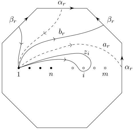
A surface can be represented as a polygon of edges with the standard identification of edges. The generators , for , are the classical braid generators on the disc. The generator , for , corresponds to the braid whose first strand goes through the edge while the rest strands are trivial. Respectively, the generator , for , corresponds to the braid whose first strand goes through the edge while the rest strands are trivial. For this geometric representation of the generators see Figure 1.
The aim of this section is to give a presentation of a certain quotient of the group . To do so, we will first give a presentation of using the short exact sequence
and standard results about presentations of group extensions. The map can be considered geometrically as forgetting the first strands of the braid. Thus, let us first state a presentation of .
Theorem 2.2 (Bellingeri, [1]).
Let . The following constitutes a presentation of .
Generators: , , , .
Relations:
, , , , as in Theorem 2.1,
-
, for , ,
-
, for , ,
-
, for , ,
-
, for , ,
-
, for .
The generators , for , and , for , are the same as in Theorem 2.1. The generator , for , corresponds to the braid whose first strand wraps around the puncture while the rest strands are trivial. For this geometric representation of the generators see Figure 1.
Remark 2.3.
Note that a braid whose first strand wraps around the puncture with the rest strands trivial can be represented by the braid corresponding to the element
For simplicity let us denote by the group and by the commutator subgroup of . From Theorem 2.2 we can deduce a presentation of , which we will use Section 3.
Corollary 2.4.
For , the following constitutes a presentation of .
Generators: , , , .
Relations:
-
All generators commute pairwise,
-
,
-
.
In particular,
where , , generate the -component and the -component.
Remark 2.5.
For simplicity, in Corollary 2.4 we denote by , , and the coset representatives of the generators , , and of , given by Theorem 2.2, in . From relation of Theorem 2.1, we get that all generators are mapped to the same element in , which we denote by . From relation of Theorem 2.1, it follows that in . Moreover, note that in the generating set we have added the generator , as we will use it in what follows, and at the same time we added in the set of relations.
We give now a presentation of the group .
Theorem 2.6.
For , the following constitutes a presentation of .
Generators:
, ,
, , .
Relations:
-
Relations , , , , , , , , of Theorem 2.2.
-
For , ,
-
for ,
for -
, for ,
, for , -
,
, -
, for ,
, for ,
, for ,
, for , -
,
-
,
for and ,
where .
-
-
For , , ,
-
,
,
, -
,
-
-
-
,
-
-
-
-
-
-
Note that the generators , and of correspond to the standard generators , and as described in Theorem 2.1, but with base point the last points, see Figure 1.

-
Proof.
In order to obtain a presentation of , we apply standard techniques for obtaining presentations of group extensions as described in [[18], p. 139] based on the following short exact sequence:
where the map can be considered geometrically as the epimorphism that forgets the first strands. For simplicity, we denote by , , the corresponding coset representatives in . The union of these elements together with the generators of of Theorem 2.2 gives us the set of generators of .
Based on [[18], p. 139] we will obtain three classes of relations in . The first class of relations is the set of relations of , that is, of , which are the relations in the class of the statement.
The second class of relations is obtained by rewriting the relations of , given in Theorem 2.1, in terms of the chosen coset representatives in and expressing the corresponding elements as a word in . Thus, we get relations in the class of the statement. The relation
of can be expressed as a word in as
and , where . This relation is obtained geometrically using the geometric representation of the generators given in Figure 1, and it corresponds to relation in the class of the statement.
The third class of relations is derived from conjugating the generators of by the coset representatives , , . The relations of this class are obtained geometrically.
-
–
By conjugating the generators , for , we obtain relations of the statement.
-
–
By conjugating the generators , for , we have relations of the statement.
-
–
By conjugating the generators , for , we have relations of the statement.
-
–
By conjugating the generators , for , we have relations of the statement.
As a result, we have obtained a generating set and a complete set of relations, which coincide with those given in the statement, and this completes the proof. ∎
-
–
3. A necessary condition for the splitting problem
In this section, we provide a necessary condition for the short exact sequence (3) to split. Let be a normal subgroup of that is also contained in . Consider the following diagram of short exact sequences:
| (4) |
where denotes the homomorphism induced by and is the canonical projection from to . Suppose that the homomorphism admits a section . Then admits a section . For , where we obtain the following short exact sequence from (4):
| (5) |
In order to study the sections of short exact sequence (5) we need a presentation of the quotients and . We already have a presentation of the Abelian group , given by Corollary 2.4. We recall that , where , , generate the -component and the -component. One can obtain a presentation of using the presentation of , given by Corollary 2.4, the presentation of given in Theorem 2.1, and once again applying standard techniques for obtaining a presentation of group extensions as described in [[18], p. 139] as presented in the proof of Theorem 2.6. However, since the group is the Abelianisation of , from the commutative diagram of short exact sequences (4), a presentation of may also be obtained straightforwardly. That is, one needs to consider the union of the generators of and the coset representatives of the generators of as a set of generators, and the relations of , given in Theorem 2.6, projected into as a set of relations, as described in the following proposition.
Proposition 3.1.
Remark 3.2.
Now, suppose that there exists a section for the homomorphism . As we already saw, it follows that there exists a section for . From Corollary 2.4, the set generates , which is the group . This allows us to describe the image of the elements of the generating set of , under the section , as follows:
| (6) |
| (7) |
| (8) |
where , for every and . Note that these integers are unique for every , and , where and . Under the assumption that there exists a section , the image of the relations, under , in are also relations in . In this way, we will obtain further information regarding the exponents in the formulas (6), (7), (8) and possible restrictions for the value of , under the assumption that the short exact sequence (3) splits.
Based on the presentation of given by Theorem 2.1, we have the following six relations, which hold in :
-
R1.
, for ,
-
, for
-
R2.
, for , ,
-
, for , ,
-
R3.
, for
-
, for
-
R4.
, for
-
, for
-
, for
-
, for
-
R5.
, for ,
-
R6.
.
In order to prove Theorem 1, we will make use of the following relations in that appear in Proposition 3.1:
For and , we have the following set of relations :
-
pairwise commute,
-
pairwise commute with ,
pairwise commute with ,
pairwise commute with ,
pairwise commute with , -
,
-
,
-
,
-
,
-
,
-
and .
Proposition 3.3.
Let , and . If the following short exact sequence
| (9) |
splits, then , where .
-
Proof.
Based on the above discussion and on the assumption that the short exact sequence (9) splits, we have that the short exact sequence (5) also splits. Thus, we will examine the relations R1-R6, which hold in , from which we will deduce that is a multiple of .
We start with the relation , for , of R1. To treat this equality, we will use the formula (6) and the relation . To simplify the calculations, in the expression of and , and in all the expressions that follow, we keep only the elements that do not commute with all the other elements. This is why we will use the symbol instead of . We can indeed ignore all the elements that commute with all the other elements since in each equality we can directly compare their exponents, since they are not affected by any possible change of position. Let . We will treat the case separately.
and similarly
Comparing the exponents of the elements and , for , of in these two equations, we obtain the following:
(10) (11) Moreover, from the equality , for , and from , , that is, commute with all the other elements in the equality, comparing the exponents of these elements, we get that:
(12) In the case where we have the following:
and similarly
Note that the exponent of the element contributes as an exponent to all the other , for , due to relation . Comparing the exponents of the elements and , for , of in these two equations, we obtain the following:
(13) (14) Moreover, from the equality and from the fact that commute with all the other elements in the equality, comparing their exponents, we get that:
(15) We continue with the second relation of R1, , for and . We will discuss the case separately. Making use of we have the following:
and similarly
Comparing the exponents of the elements and , for and , of in these two equations, we obtain the following:
(16) In the case where and we have the following:
and similarly
Note that the exponent of the element contributes as an exponent to all the other , for , due to relation . Comparing the exponents of the elements and , for , of in these two equations, we obtain the following:
(17) (18) Thus, from the obtained relations and we set
It follows that the relation 6 becomes
(19) We continue with the relation , for and , of R2. We will discuss the case separately. So, for , based on the formulas (19), (7) and the relations , we have the following:
and
Comparing the coefficients of the element , and , for of in these two equations, it follows that
(20) and
(21) In the case we have the following:
and
Note that the exponent of the element contributes as an exponent to all the other , for , due to relation . Comparing the coefficients of the element , it follows that
(22) Similarly, from the relation of R2, , for and , and with the use of the relation , we get that
(23) and
(24) In addition, for from the relation , for , it follows that
(25) The calculation of the remaining relations R3, R4 and R5 is straightforward and we present directly the results one will obtain. However, the last relation R6 will be presented in detail.
From the relation of R3, , for and using the relations , , comparing the exponents of the element we get that
(26) From the relation of R3, , for and using the relations , , comparing the exponents of the element we obtain that
(27) From the relation of R4, , for , and using the relations , , comparing the exponents of the elements and we obtain that
(28) From the relation of R4, , for and using the relations , , , comparing the exponents of the elements and we obtain that
(29) and
(30) From the relation of R4, , for and using the relations , , comparing the exponents of the elements and we obtain that
(31) From the relation of R4, , for and using the relations , , , comparing the exponents of the elements and we obtain that
(32) and
(33) From the relation of R5, , for , and using the relations , , , comparing the exponents of the elements and , for we obtain that
(34) (35) and
(36) We now analyse the results that we obtained so far. From (20), (23) we obtain and , for all . From (20), (17), (36) it follows that , for and . In addition, from (10), (13), (18) it follows that , for and . All together we get that , for and . That it, and , for . From (26), (28) we have , for all . Moreover, from (29), (33) we get , for . From (27), (31) we get , for all and from (30), (32) we have , for . From (21), (22) it follows that , for and . Similarly from (24), (25) it follows that , for and . From (18) it holds that , which integer we will denote by . From (34), (35) we have , which integer we will denote by . For simplicity, we will now denote by , for and similarly, by , for . Lastly, from (11), (14) we obtain that .
Finally, with these new images of , and , under , we will examine the relation R6, . Note that . We will compute the image of and of separately, making use of the relation .
Similarly,
Therefore,
Moreover, with the use of the relations , we have the following:
From we have that in . Therefore,
Thus, .
Comparing the exponents of the element of the equality we obtain the following: . That is,
We deduce that , for , which concludes the proof. ∎
Remark 3.4.
For and , using the the same strategy as in the proof of Proposition 3.3 we obtain that , for . In particular, we examine the relations R3-R6, since the relations R1-R2 do not hold for .
For and , using the the same strategy as in the proof of Proposition 3.3 we obtain that , for . In particular, we examine the relations R1-R6, except for the relation of R1, for , which does not hold for .
For and , using the the same strategy as in the proof of Proposition 3.3 we obtain that , for . In particular, we examine the relations R3, R5, R6, since the relations R1, R2, R4 do not hold for and .
For and , using the the same strategy as in the proof of Proposition 3.3 we obtain that , for . In particular, we examine the relations R1-R6, except for the relation of R1, for , and the set of relations of R4, which does not hold for and .
For and , using the the same strategy as in the proof of Proposition 3.3 we obtain that , for , examining the relations R1-R6, except for the set of relations of R4, which does not hold for .
In the following proposition we provide a geometric section from which we can deduce an algebraic section for , using a similar construction, given by Gonçalves–Guaschi in [13], the case of pure braid groups.
Proposition 3.5.
Let , and . The short exact sequence
| (37) |
splits for all values of and .
-
Proof.
Let , and . In order to provide an algebraic section for the map we will construct a geometric section in the level of configuration spaces, see Remark 1.1. That is, we will present a section for the map , defined by forgetting the first coordinates. We construct such a section in the following way.
We known that there exists a circle on that is a retract of . That is, for , the inclusion of into , there exists a continuous map , such that, for every , and . We take to be any meridian of one of the handles of . Thus, for such a choice of there exists indeed a retraction of onto , since is a non-separating circle of as it is one of the meridians.
Using this retraction, we will define pairwise coincidence-free continuous self maps of . For , we define to be , the composition of the retraction with the rotation of of angle . With the rotation we ensure that for every point it holds that and , for all such that and . Thus, the following continuous self maps of , , are pairwise coincidence-free.
Thus, by setting we construct a continuous map from to , that is indeed a geometric section since . As a result, we deduce, for all and , a section for the map .
∎
4. Jenkins–Strebel quadratic differentials
In this section we will introduce the notion of Jenkins–Strebel quadratic differentials which induce a unique ribbon graph on a Riemann surface. This will be the main tool that we will use in the following section to construct geometric sections. The main references for this section are [19] and [8].
Given a Riemann surface of genus with marked points on it, and given positive real numbers , called perimeters, Strebel’s theorem [21] claims that there exists a unique Strebel quadratic differential with double poles at the marked points with residues equal to .
A quadratic differential on a Riemann surface is a meromorphic section of the tensor square of the cotangent bundle. Locally, in every chart , with local coordinates , is of the form , where is a meromorphic function in . The set of zeroes and poles of a quadratic differential, which is not identically zero, is finite. The complement to the set of zeroes and poles is equipped with the horizontal and the vertical line field. The horizontal line field determined by vectors such that the value of on them is positive real. Similarly, the vertical line field determined by vectors such that the value of on them is negative real. The Jenkins–Strebel quadratic differentials are quadratic differentials that have at most double poles, with negative residues, such that all horizontal trajectories except for a finite set are closed. In that case, the set of horizontal trajectories which are non-closed is an embedded graph onto .
Before stating Strebel’s theorem, we recall the notion of a ribbon graph. A ribbon graph or an embedded graph is a connected graph equipped with a cyclic order of the half-edges issuing from each vertex. It is a standard fact that any given cyclic order allows one to construct a unique embedding of the graph into a surface. If an abstract graph is embedded into a surface, the cyclic order of the half-edges adjacent to a vertex is just the counterclockwise order.
Theorem 4.1 (Strebel, [21]).
Given an orientable compact Riemann surface of genus , with distinct points, on and an -tuple of positive real numbers, if , then there exists a unique Strebel differential with double poles at with residues respectively. The non-closed horizontal trajectories of the Strebel differential form a unique ribbon graph on the Riemann surface , whose faces are topological discs surrounding the marked points , for and the perimeter, measured with the metric , of the -th face is .
The vertices of the graph are the zeroes of an arbitrary order of the differential. At a zero of order , due to the local representation of the quadratic differential, there are horizontal trajectories meeting at such a point. Thus, the valency of each vertex of the graph is not less than three.
In the generic case, when all the vertices are of degree three, then the graph has edges. This follows from the fact that two times the number of edges equals three times the number of vertices and the fact that the Euler characteristic is , which is equal to the number of faces and vertices minus the number of edges. Therefore, to a Riemann surface with marked points, and perimeters , we can associate a unique metric ribbon graph with edge lengths , measured with the metric . The converse is true as well. That is, given a ribbon graph of genus with faces, and given the lengths of its edges, we can reconstruct a unique Riemann surface with marked points, by gluing conformally discs along the edges of the ribbon graph, as well as positive real numbers , where is the sum of the lengths of the edges that surround the -th face. Therefore, because of the uniqueness of the Strebel differential, we have the following bijection, where by we denote the Moduli space of orientable compact Riemann surfaces of genus , with distinct labeled marked points. That is, .
Theorem 4.2.
We have the following isomorphism of orbifolds.
5. Geometric construction of sections
In this section we will construct geometric sections for the fibration , proving Theorem 2.
-
Proof of Theorem 2.
Let be an orientable compact surface of genus and a set of distinct points on . Given a Riemann structure on and an -tuple of perimeters , we know from Strebel’s theorem 4.1 that there exists a unique Strebel differential , which defines a unique ribbon graph on the Riemann surface with faces that correspond to topological discs surrounding the given points . Before choosing the -tuple of we need to give an ordering to the set . Without loss of generality we consider the following ordering . Since in fact the given distinct points on the surface are not ordered, the structure of the ribbon graph should not depend on the ordering that is given to the points. Thus, whatever ordering would have been given to the -point set, the perimeters that would be assigned to each point should be the same. To achieve that, for any permutation of the given -point set we associate the corresponding permutation of . That is, the -tuple of perimeters that will be assigned to the -tuple will be , where is an element of the symmetric group of degree .
It is known that the subset of the parameter space inside that gives a trivalent graph is open dense [16]. Therefore, we can always choose a Riemann structure on and an -tuple of perimeters in such a way that the obtained unique ribbon graph will be in fact trivalent. Thus, for and we choose a Riemann structure and an -tuple of perimeters such that the unique ribbon graph we will obtain on is a trivalent graph. In this case, the ribbon graph has faces, edges and vertices, as explained in Section 4. On this ribbon graph we can now construct new distinct unordered points. In particular, along each edge of the ribbon graph we take equally-spaced new points (for we take the midpoint), where , that are clearly different from the initial points. With this construction we obtain new distinct points along the edges of the ribbon graph as well as new distinct points that correspond to the vertices of the ribbon graph. In addition, from Theorem 4.2 it follows that the construction of these new, distinct points depends continuously on the given -points . That is, when we let the complex structure and the marked points vary, the map that associates to a Riemann surface with marked points a metric ribbon graph is continuous. Thus, we can conclude that the fibration admits a section for and , where . ∎
Remark 5.1.
Note that for the above mentioned construction we let the Riemann structure on vary. However, this does not affect the construction of the sections of the fibration . The reason is that the Fadell–Neuwirth fibration is purely topological and exists independently of any complex structure on the surface. That is, it only depends on the topological structure of the surface and the topology of remains the same for any Riemann structure on it.
6. Geometric sections for the 2-sphere
In this section we will focus now on the case of the 2-sphere.We will prove Theorem 3 and we will compare this result with already known results on geometric sections on the 2-sphere. In the case where we assume that in order to apply Theorem 4.1.
We want to compare this result with the results obtained by Gonçalves–Guaschi [15] and Chen–Salter [5] concerning the construction of geometric sections on the 2-sphere. In [15], Gonçalves–Guaschi do not consider any Riemann structure on the 2-sphere. In [5], Chen–Salter, in some cases, view the 2-sphere as the projective space .
Theorem 6.1 (Gonçalves–Guaschi, [15]).
A group-theoretic section exists if and only if or .
Theorem 6.2 (Chen–Salter, [5]).
For any and for any divisible by , there is a section .
Theorem 6.3 (Chen–Salter, [5]).
No section exists for unless divides .
Considering the equivalence between the group-theoretic sections with the geometric ones, see Remark 1.1, we see that for Theorem 3 agrees with Theorem 6.1. Moreover, from Theorem 3, for and choosing , we obtain a section for , which agrees with Theorem 6.2. However, from Theorem 3 we obtain more sections that presented in Theorem 6.3. In particular, they state that for there exists no section unless is a multiple of . From our result when we obtain a section for , but in addition we can construct sections for and for , where . These additional sections are due to the fact that we allow the Riemann structure of the 2-sphere vary as the marked points vary.
Remark 6.4.
It is important to note that for no geometric section has been constructed so far of the fibration . In our setting, where we equip the 2-sphere with a Riemann structure and let it vary while the 5 marked point vary, from Theorem 3, we can construct geometric sections of for , and , where .
Acknowledgement
The author gratefully acknowledges the Max Planck Institute for Mathematics in Bonn for its hospitality and financial support during a research stay, which enabled the initial phase of this research project. In addition, the author is grateful to Jijian Song and to Alessandro Giacchetto for their valuable insights and knowledge on Jenkins–Strebel quadratic differentials.
References
- [1] P. Bellingeri. On presentations of surface braid groups. J. Algebra, 274:543–563, (2004).
- [2] P. Bellingeri, E. Godelle, and J. Guaschi. Exact sequences, lower central series and representations of surface braid groups. arXiv:1106.4982.
- [3] J. S. Birman. On braid groups. Comm. Pure Appl. Math., 22:41–72, (1969).
- [4] L. Chen. Section problems for configuration spaces of surfaces. Journal of Topology and Analysis, 13:469–497, (2021).
- [5] L. Chen and N. Salter. Section problems for configurations of points on the Riemann sphere. Algebr. Geom. Topol., 20:3047–3082, (2020).
- [6] W. Chen. Obstructions to choosing distinct points on cubic plane curves. Advances in Mathematics, 340:211–220, (2018).
- [7] C. J. Earle and I. Kra. On sections of some holomorphic families of closed Riemann surfaces. Acta Mathematica, 137:49 – 79, (1976).
- [8] B. Eynard. Counting Surfaces. Progress in Mathematical Physics. Birkhäuser Basel, (2016).
- [9] E. Fadell. Homotopy groups of configuration spaces and the string problem of Dirac. Duke Math. J., 29:231–242, (1962).
- [10] E. Fadell and L. Neuwirth. Configuration spaces. Math. Scand., 10:111–118, (1962).
- [11] E. Fadell and J. Van Buskirk. The braid groups of and . Duke Math. J., 29:243–257, (1962).
- [12] R. Fox and L. Neuwirth. The braid groups. Math. Scand., 10:119–126, (1962).
- [13] D. L. Gonçalves and J. Guaschi. On the structure of surface pure braid groups. J. Pure Appl. Algebra, 186:187–218, (2004).
- [14] D. L. Gonçalves and J. Guaschi. Braid groups of non-orientable surfaces and the Fadell–Neuwirth short exact sequence. J. Pure Appl. Algebra, 214:667–677, (2010).
- [15] D. L. Gonçalves and J. Guaschi. The braid group and a generalisation of the Fadell-Neuwirth short exact sequence. J. Knot Theory Ramifications, 14:375–403, (2005).
- [16] J. L. Harer. The cohomology of the moduli space of curves. In Theory of Moduli, pages 138–221. Springer Berlin Heidelberg, (1988).
- [17] J. H. Hubbard. Sur les sections analytiques de la courbe universelle de teichmüller. American Mathematical Society, (1976).
- [18] D. L. Johnson. Presentations of groups. London Mathematical Society Student Texts, Vol. 15. Cambridge University Press, Cambridge, (1997).
- [19] S. Lando and A. Zvonkin. Graphs on Surfaces and Their Applications. Encyclopaedia of mathematical sciences, Vol. 141. Springer-Verlag, Berlin, (2004).
- [20] S. Makri. The braid groups and the splitting problem of the generalised Fadell–Neuwirth short exact sequence. Topology Appl., 318:108202, (2022).
- [21] K. Strebel. Quadratic differentials. Springer-Verlag, (1984).
- [22] J. Van Buskirk. Braid groups of compact 2-manifolds with elements of finite order. Trans. Amer. Math. Soc., 122:81–97, (1966).