Understanding Generalization of Federated Learning:
the Trade-off between Model Stability and Optimization

Abstract

Federated Learning (FL) is a distributed learning approach that trains neural networks across multiple devices while keeping their local data private. However, FL often faces challenges due to data heterogeneity, leading to inconsistent local optima among clients. These inconsistencies can cause unfavorable convergence behavior and generalization performance degradation. Existing studies mainly describe this issue through convergence analysis, focusing on how well a model fits training data, or through algorithmic stability, which examines the generalization gap. However, neither approach precisely captures the generalization performance of FL algorithms, especially for neural networks. In this paper, we introduce the first generalization dynamics analysis framework in federated optimization, highlighting the trade-offs between model stability and optimization. Through this framework, we show how the generalization of FL algorithms is affected by the interplay of algorithmic stability and optimization. This framework applies to standard federated optimization and its advanced versions, like server momentum. We find that fast convergence from large local steps or accelerated momentum enlarges stability but obtains better generalization performance. Our insights into these trade-offs can guide the practice of future algorithms for better generalization.

Introduction

Federated Learning (FL) has become a new solution for training AI models on distributed and private data (McMahan et al. 2017). Traditional centralized learning approaches require data to be gathered in one place, posing risks to privacy and security (Voigt and Von dem Bussche 2017; Li, Yu, and He 2019; Zhang et al. 2023). In response, FL allows models to be trained directly on local devices, keeping raw data decentralized. This paradigm has enabled many applications in fields like healthcare (Antunes et al. 2022), finance (Long et al. 2020), and IoT (Nguyen et al. 2021), where protecting sensitive data is crucial. However, FL often faces significant performance challenges due to heterogeneous data in real-world scenarios. Many experimental and theoretical results of FL have observed that the heterogeneity issues degenerate the FL performance on both training behavior and testing accuracy (Huang et al. 2023). Therefore, numerous studies in FL have been proposed to alleviate the negative impacts of heterogeneity.

However, most existing studies of FL only emphasize convergence to empirical optimal solutions based on training datasets (Reddi et al. 2020; Wang, Lin, and Chen 2022; Li et al. 2019) and usually ignore their generalization properties. In response, recent generalization studies of FL (Sun, Niu, and Wei 2024; Sun, Shen, and Tao 2024) raise this important issue of generalization in the FL community. Although their generalization analysis is established on the most popular technique called Uniform Stability (Hardt, Recht, and Singer 2016), they usually do not work well under general non-convex regimes (Chen, Jin, and Yu 2018; Charles and Papailiopoulos 2018; Zhou, Liang, and Zhang 2018), because it depends heavily on the gradient norm (Li, Luo, and Qiao 2019). Unfortunately, neural networks, the most advanced techniques in the era of artificial intelligence, are non-convex. Therefore, understanding the generalization of FL under non-convex regimes is essential for future applications.

Analyzing the generalization dynamics is a feasible solution to understanding the generalization of non-convex FL (Teng, Ma, and Yuan 2021). This generalization dynamics is to measure the generalization gap during the neural networks training process. However, the previous uniform stability analyses are less practical. They ignored the gradient norm dynamics in neural network training which is non-zero. On the other hand, the convergence analysis of non-convex FL only focuses on the gradient norm, however, omits the generalization dynamics. Therefore, the existing approach cannot precisely describe the generalization properties.

In this paper, we propose a novel stability-based analysis framework of jointly analyzing training dynamics of model stability and optimization for a non-convex FL training process, as stated in Corollary 1 and illustrated in Figure 1. Through this framework, we suggest the model stability and optimization trade-off in the generalization performance of FL. And, we obtain the upper bound of optimal generalization performance for an FL training process by resolving the trade-off. Our results suggest the importance of a global learning rate selection strategy for mitigating overfitting. We summarize our contributions as follows:

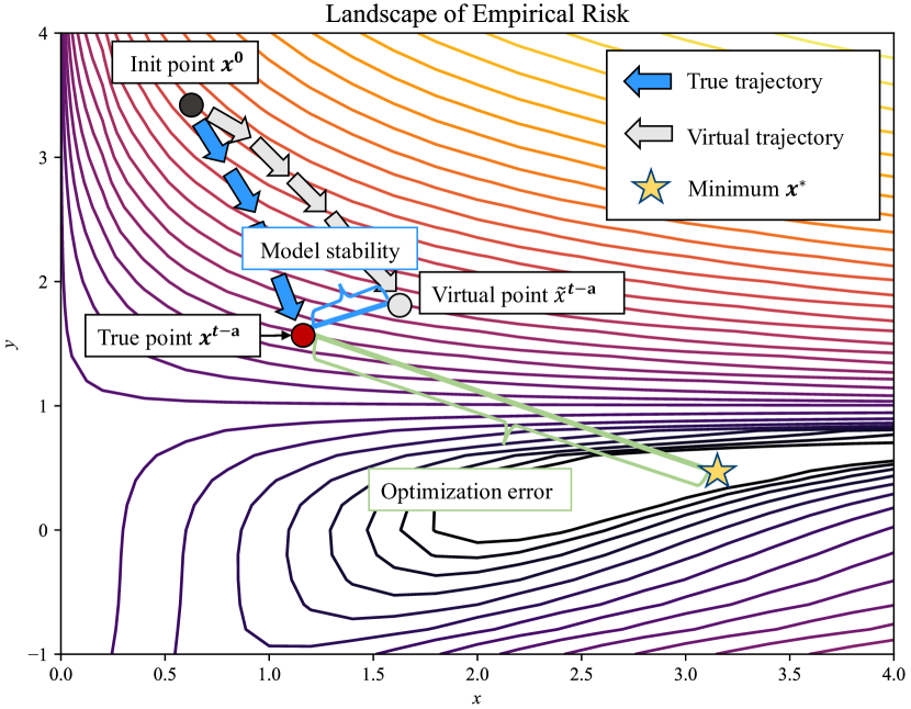
(a) Under-fitting

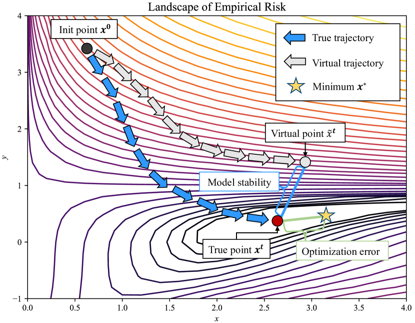
(b) Benign-fitting

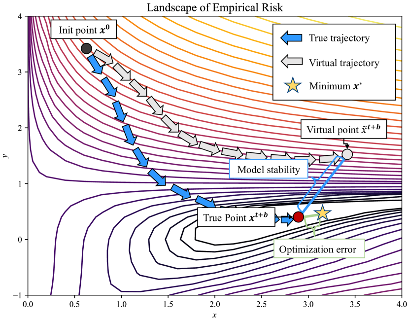
(c) Over-fitting

Figure 1: Key Idea: understand generalization dynamics via jointly analyzing model stability and optimization error. Corollary 1 shows that the excess risk is roughly bounded by optimization error (green line) and model stability (blue line). In a training process, the green line shrinks, and the blue line expands at different speeds. At an early stage, the optimization error dominates the excess risk bound indicating under-fitting. When the model stability dominates the excess risk, the model becomes over-fitting. We identify the properties of benign-fitting about $t$ by jointly analyzing model stability and optimization error.

• We propose a novel theoretical framework that precisely describes the excess risk bound for FL algorithms under non-convex regimes. This framework focuses on analyzing the trade-offs between model stability and optimization error. And, our primary results contribute new understandings on the global learning rate in FL.

• Our theories identify key factors affecting generalization performance. Specifically, we find that optimization acceleration techniques, such as using large local update steps and server momentum, worsen the model stability. Despite that, they can implement tighter excess risk bound by obtaining more benefits from optimization.

• Empirically, we evaluate our theories in standard federated learning settings. Our results provide valuable insights for FL practices.

Related Work

Generalization theory

Generalization in learning theory has been a focus for decades. Uniform convergence, which uses VC dimension or Rademacher complexity to bound generalization error, is a common approach (Shalev-Shwartz et al. 2010; Yin, Kannan, and Bartlett 2019). However, this method often provides less meaningful bounds for neural networks (Zhang et al. 2021) because it only considers the model class, not the training algorithms used to generate the models. PAC-Bayes learning is another valuable approach for analyzing generalization errors in neural networks (Dziugaite and Roy 2017). It has been used to analyze bounds for stochastic optimization algorithms (Pensia, Jog, and Loh 2018; Neu et al. 2021). Similar to the PAC-Bayes framework, algorithmic stability is increasingly used in recent analyses of randomized learning algorithms (Hardt, Recht, and Singer 2016; Lei and Ying 2020). This concept measures how sensitive the loss function is to changes in the training data. Stability analysis has been extended to various areas, including randomized learning algorithms (Elisseeff et al. 2005), transfer learning (Kuzborskij and Lampert 2018), and privacy-preserving learning (Dwork and Feldman 2018). It is able to derive tighter generalization bounds in expectation.

Generalization theory in FL

Many works have studied the properties of generalization in FL. Most works derived PAC-Bayes or information-theoretic bounds for the general FL paradigm using the Donsker-Varadhan variational representation (Wu et al. 2023a, b; Barnes, Dytso, and Poor 2022). Based on the theories, corresponding works (Reisizadeh et al. 2020) mainly developed robust FL methods to enhance generalization performance against heterogeneous clients. Moreover, Qu et al. (2022) proposes to improve the flatness of loss landscape by adopting the sharpness aware minimization (SAM) optimizer on FL. Follow-up works (Caldarola, Caputo, and Ciccone 2022; Sun et al. 2023; Shi et al. 2023) propose some variants based on SAM that can improve FL performance. However, these works only focus on the final generalization performance of the FL model, while ignoring the training dynamics during the federated learning procedure. Hence, there are lack of understanding of key factors affecting the generalization errors at the algorithm level. To the best of our knowledge, only two works provide explicit analysis for algorithmic stability in FL. Sun, Niu, and Wei (2024) provides a straightforward extension of work (Hardt, Recht, and Singer 2016) for FedAvg (McMahan et al. 2017), FedProx (Li et al. 2020), and SCAFFOLD (Karimireddy et al. 2020), highlighting the impacts of data heterogeneity on generalization. Sun, Shen, and Tao (2024) mainly prove the stability of the proposed algorithm FedInit and show its generalization error bound is also dominated by heterogeneity issues. And, FedInit simply plus optimal convergence rate and stability for denoting excess risk bound. However, the optimal convergence rate and stability cannot obtained simultaneously as they rely on different hyperparameters of the training algorithm. Hence, it omitted the interplay between convergence and stability, making previous results inaccurately guide neural network training.

Problem Formulation

In this section, we introduce the necessary definitions and previous techniques.

Consider a standard FL setting with $N$ clients connected to one aggregator. The basic problem in FL is to learn a prediction function parameterized by $\boldsymbol{x}\in\mathcal{X}\subseteq\mathbb{R}^{d}$ to minimize the following global population risk:

$$F(\boldsymbol{x}):=\frac{1}{N}{\sum}_{i=1}^{N}\mathbb{E}_{z\sim\mathcal{P}_{i}}[\ell(\boldsymbol{x};z)],$$ (1)

where $\mathcal{P}_{i}$ is the underlying data distribution on client $i$ and may differ across different clients, $\ell(\boldsymbol{x};z):\mathcal{X}\times\mathcal{Z}\rightarrow\mathbb{R}^{+}$ is some nonnegative loss function, $z$ denotes the sample from the sample space $\mathcal{Z}$.

Since $\mathcal{P}_{i}$ is unknown typically, the global population risk $F(\boldsymbol{x})$ cannot be computed. Instead, we can access to a training dataset $\mathcal{D}=\cup_{i=1}^{N}\mathcal{D}_{i}$, where $\mathcal{D}_{i}=\{z_{j}^{(i)}\}_{j=1}^{n_{i}}$ is the training dataset on client $i$ with size $n_{i}$. Then, we can estimate $F(\boldsymbol{x})$ using global empirical risk:

$$f(\boldsymbol{x}):=\frac{1}{N}{\sum}_{i=1}^{N}f_{i}(\boldsymbol{x}),$$ (2)

where $f_{i}(\boldsymbol{x})=\frac{1}{n_{i}}\sum_{j=1}^{n_{i}}\ell(\boldsymbol{x};z_{j}^{(i)})$ is the local empirical risk on client $i$, $z_{j}^{(i)}\overset{\text{ i.i.d. }}{\sim}\mathcal{P}_{i}$ represents the sample from local data distribution $\mathcal{P}_{i}$.

In practice, a family of algorithms to solve (2) has been proposed (Hsu, Qi, and Brown 2019; Reddi et al. 2020; Xu et al. 2021; Zeng et al. 2023b; Wang et al. 2020), which take form:

Client: $$\quad\boldsymbol{x}_{i}^{t,k+1}=\textsc{ClientOpt}(\boldsymbol{x}_{i}^{t,k},\boldsymbol{g}_{i}^{t,k},\eta_{l});$$

Server: $$\quad\boldsymbol{x}^{t+1}=\textsc{ServerOpt}(\boldsymbol{x}^{t},\boldsymbol{d}^{t},\eta_{g}),$$

where ClientOpt and ServerOpt are gradient-based optimizers with learning rates $\eta_{l}$ and $\eta_{g}$ respectively. Essentially, ClientOpt aims to minimize the loss on each client’s local data with stochastic gradient $\boldsymbol{g}_{i}^{t,k}$, while ServerOpt updates the global model based on the aggregated clients’ model updates $\boldsymbol{d}^{t}$. For the simplicity of the following analysis, we assume that both ClientOpt and ServerOpt are in the form of SGD. See Algorithm 1 for more details.

Excess risk

Understanding the mechanism of this basic FL algorithm is vital for designing efficient and generalizable algorithms (Sun, Shen, and Tao 2024; Teng, Ma, and Yuan 2021). To this end, we are interested in the excess risk $\tilde{\mathcal{E}}(\boldsymbol{x}):=F(\boldsymbol{x})-F(\boldsymbol{x}^{*})$, where $\boldsymbol{x}^{*}:=\min_{\boldsymbol{x}\in\mathcal{X}}F(\boldsymbol{x})$ denotes the population risk minimizer. Noting that the excess risk measures how the learned parameter $\boldsymbol{x}$ performs on the population risk, it can be decomposed as

$$\tilde{\mathcal{E}}(\boldsymbol{x}) =F(\boldsymbol{x})-f(\boldsymbol{x})+f(\boldsymbol{x})-f(\hat{\boldsymbol{x}})$$ (3)

$$\quad+\underbrace{f(\hat{\boldsymbol{x}})-f(\boldsymbol{x}^{*})}_{\leq 0\text{ under ERM }}+\underbrace{f(\boldsymbol{x}^{*})-F(\boldsymbol{x}^{*})}_{\approx 0~{}\text{by concentration inequality}},$$

where $\hat{\boldsymbol{x}}$ denotes the empirical risk minimizer (ERM). Empirically, the last two terms of the above equation are algorithm-independent (Teng, Ma, and Yuan 2021). To provide deeper insights on neural networks training, we prefer to study the empirical excess risk related to learned parameter $\boldsymbol{x}$:

$$\mathcal{E}(\boldsymbol{x})=\underbrace{F(\boldsymbol{x})-f(\boldsymbol{x})}_{\mathcal{E}_{G}:\text{ generalization gap}}+\underbrace{f(\boldsymbol{x})-f(\hat{\boldsymbol{x}})}_{\mathcal{E}_{O}:\text{ optimization error }},$$ (4)

where the first term $\mathcal{E}_{G}$ denotes the estimation error due to the approximation of the unknown data distribution $\mathcal{P}$. The second term $\mathcal{E}_{O}$ means the optimization error based on training data $\mathcal{D}$.

Algorithm 1 Federated Optimization(Reddi et al. 2020)

0:  $\boldsymbol{x}^{0},\eta_{l},\eta_{g},T$

0:  $\boldsymbol{x}^{T}$

1:  for round $t$ $\in$ $[T]$ do

2:     Server broadcast model $\boldsymbol{x}^{t}$ to clients

3:     for client $i$ $\in$ $[N]$ in parallel do

4:        $\boldsymbol{x}^{t,0}_{i}=\boldsymbol{x}^{t}$

5:        for local update step $k=0,\dots,K-1$  do

6:           $\boldsymbol{x}^{t,k+1}_{i}=\boldsymbol{x}^{t,k}_{i}-\eta_{l}\boldsymbol{g}_{i}^{t,k}$

7:        end for

8:        Client uploads local updates $\boldsymbol{d}_{i}^{t}=\boldsymbol{x}^{t,0}-\boldsymbol{x}^{t,K}$

9:     end for

10:     Server compute an estimate $\boldsymbol{d}^{t}=\frac{1}{N}\sum_{i\in[N]}\boldsymbol{d}_{i}^{t}$

11:     Server updates $\boldsymbol{x}^{t+1}=\boldsymbol{x}^{t}-\eta_{g}\boldsymbol{d}^{t}$

12:  end for

Establishing Excess Risk Dynamics

This section formally describes the concept of excess risk dynamics, which is derived from algorithmic stability.

Algorithmic stability is one of the most popular theoretical frameworks for analyzing generalization gap (Hardt, Recht, and Singer 2016; Lei and Ying 2020). Our analysis relies on the on-average model stability (Lei and Ying 2020), which gives tighter bounds than uniform stability (Hardt, Recht, and Singer 2016). In detail, model stability means any perturbation of samples across all clients cannot lead to a big change in the model trained by the algorithm in expectation. Formally, the upper bound of generalization gap $\mathcal{E}_{G}(\boldsymbol{x})$ is related to model stability:

Theorem 1 (Modified generalization gap).

Let $\mathcal{D},\mathcal{D}^{\prime}$ differ in at most one data sample (perturbed sample). For the two models $\boldsymbol{x}$ and $\tilde{\boldsymbol{x}}$ trained by a learning algorithm on these two sets, if function $f$ is $L$-smooth, the generalization gap is upper bounded:

$$\mathcal{E}_{G}(\boldsymbol{x})\leq\frac{L+\gamma}{2}\underbrace{\mathbb{E}_{\mathcal{D},\mathcal{D}^{\prime}}[\|\boldsymbol{x}-\tilde{\boldsymbol{x}}\|^{2}]}_{\text{Model stability}}+\frac{1}{2\gamma}\mathbb{E}_{\mathcal{D}}\|\nabla f(\boldsymbol{x})\|^{2},$$ (5)

where $\gamma>0$ is a free parameter for tuning depending on the property of problems.

Remark.

Compared with the original theory (Theorem 2 in paper (Lei and Ying 2020)), we removed the Holder continuity assumption and replaced the empirical loss term with the gradient norm. We provide rigorous proof in Appendix A. Under the Holder-continuity condition, the model stability dominates the generalization gap $\mathcal{E}_{G}$ since $\mathcal{E}_{O}$ is minor. Hence, the original theory proves that if an algorithm is stable, its excess risk is small. In contrast, this modified theorem shows that the generalization gap is also subjected to the gradient norm, which is overlooked. Furthermore, the gradient norm $\mathbb{E}\|\nabla f(\boldsymbol{x})\|^{2}$ typically is non-zero in neural network training practices. Therefore, omitting the effects of gradient norms can be a drawback of algorithmic stability analysis.

Here, we introduce a novel quantity termed excess risk dynamics for generalization analysis:

Corollary 1 (Excess risk dynamics).

Under conditions of Theorem 1, an training algorithm creates a model trajectory $\{\boldsymbol{x}^{t}\}_{t=0}^{T}$ on dataset $\mathcal{D}$, and a virtual trajectory $\{\tilde{\boldsymbol{x}}^{t}\}_{t=0}^{T}$ on datasets $\mathcal{D}^{\prime}$. Under the condition of Theorem 1, substituting (4) with (5) and using $\mathcal{E}_{O}(\boldsymbol{x}^{t})\leq\frac{1}{2\mu}\mathbb{E}\|\nabla f(\boldsymbol{x}^{t})\|^{2}$ ($\mu$-PL condition), we have the excess risk bound consisting of model stability and gradient norm as

$$\mathcal{E}(\boldsymbol{x}^{t})\leq\frac{L+\gamma}{2}\underbrace{\mathbb{E}\|\boldsymbol{x}^{t}-\tilde{\boldsymbol{x}}^{t}\|^{2}}_{\text{Model stability}}+(\frac{1}{2\gamma}+\frac{1}{2\mu})\underbrace{\mathbb{E}\|\nabla f(\boldsymbol{x}^{t})\|^{2}}_{\text{Gradient norm}}.$$

The gradient norm of the non-convex training process is related to its convergence status. To see this, we assume the risk $f$ is $\mu$-PL condition, which is a practical assumption in non-convex functions (Jain, Kar et al. 2017). As the empirical optimal $\boldsymbol{x}^{*}$ typically considered unknown in the non-convex analysis, it allows us to use the gradient norm $\mathbb{E}\|\nabla f(\boldsymbol{x})\|^{2}$ to bound the optimization error $\mathcal{E}_{O}(\boldsymbol{x})$.

Remark (Conflicts between stability and gradient norm).

The model stability and gradient norm conflict in excess risk bound as illustrated in Figure 1. Concretely, the stability expands while the gradient norm decreases over model iteration. From the generalization perspective, we expected the model stability bounds to grow slowly (e.g., vanilla SGD typically grows at a speed of $\mathcal{O}(T^{c})$ (Hardt, Recht, and Singer 2016)). That is, a smaller difference between the true sequence and the virtual sequence indicates better model stability and lower generalization gap. In contrast, the gradient norm should decrease fast in non-convex convergence analysis, indicating that the model is fitting training datasets well. Typically, the convergence speed should roughly match $\mathcal{O}(1/\sqrt{T})$ (Reddi et al. 2020).

Given the conflicts, the exact bound under the trade-off has not been fully characterized. Inspired by trajectory analysis (Jin et al. 2021), we aim to bound the minimum excess risk of a model training procedure as follows:

Definition 1 (Minimum excess risk dynamics).

Given a training procedure yielding a model trajectory $\{\boldsymbol{x}\}_{t=0}^{T}$, there is a particular time point that the model achieves the minimum excess risk value over all time. We define the excess risk at the exact time as the minimum excess risk termed as $\mathcal{E}_{\text{min}}=\min_{t\in[T]}\mathcal{E}(\boldsymbol{x}^{t})$.

Understanding the minimum excess risk bound is to identify the key factors that affect the generalization. It is also crucial to design FL algorithms that are both efficient and generalizable, which is the primary motivation for this work. In the technical part of this paper, we first introduce a federated model stability analysis framework in the next section. Then, we jointly analyze the stability and gradient norm dynamics.

Federated Model Stability Analysis

In this section, we provide the model stability analysis of Algorithm 1 with detailed proof provided in Appendix B. Our further analysis relies on some common assumptions on local stochastic gradients (Reddi et al. 2020; Sun, Shen, and Tao 2024; Zeng et al. 2023b):

Assumption 1.

The stochastic gradient $\boldsymbol{g}_{i}$ (Line 6 in Algorithm 1) is unbiased, i.e.,$\mathbb{E}\left[\boldsymbol{g}_{i}\right]=\nabla f_{i}(\boldsymbol{x})$. And, the variance of $\boldsymbol{g}_{i}$ is $\sigma_{l}$-bounded (local) variance as $\mathbb{E}\left[\left\|\boldsymbol{g}_{i}-\nabla f_{i}(\boldsymbol{x})\right\|^{2}\right]\leq\sigma_{l}^{2}$, for all $i\in[N],z\in\mathcal{D}_{i}$. Here, the expectation is taken over the randomness of SGD.

Assumption 2.

The global variance is bounded as $\mathbb{E}\left\|\nabla f_{i}(\boldsymbol{x})-\nabla f(\boldsymbol{x})\right\|^{2}\leq\sigma_{g}^{2}$ for all $i$ and $x\in\mathcal{X}$.

Now, we describe the main steps of establishing the federated model stability.

Outline of proof

The Algorithm 1 consists of local multi-step SGD and global SGD. To prove the algorithm is stable, we should identify how true global sequence and virtual global sequence differ due to the perturbed sample (Hardt, Recht, and Singer 2016). Although we focus on the stability of the global model, the data are preserved for local clients in FL. Thus, the federated model stability analysis should first measure the divergence of local updates due to the perturbed sample. Concretely, we prove the local stability expands each round with a coefficient, which is proportional to local gradient variance $\sigma_{l}^{2}$, global variance $\sigma_{g}^{2}$, and local update steps $K$. Then, after the local updates are used to update the global model, the global model inherits the expansive property:

Lemma 1 (Expansion of federated model stability).

Under conditions of Corollary 1 and Assumptions 1 2., if all clients use identical local update step $K$, batch size $b$ and $\eta_{l}=\Theta(\frac{1}{KL})$ for local mini-batch SGD, we denote $\{\boldsymbol{x}^{t}\}_{t=0}^{T}$ is the main trajectory of global model generated by the Algorithm 1 on dataset $\mathcal{D}$. And, $\{\tilde{\boldsymbol{x}}^{t}\}_{t=0}^{T}$ is the virtual trajectory of the global model trained on datasets $\mathcal{D}^{\prime}$. For a free parameter $p>0$, the global model stability is expansive in expectation as:

$$\mathbb{E}\|\boldsymbol{x}^{t+1}-\tilde{\boldsymbol{x}}^{t+1}\|^{2} \leq(1+p)(1+\psi\eta_{g}^{2})\mathbb{E}\|\boldsymbol{x}^{t}-\tilde{\boldsymbol{x}}^{t}\|^{2}$$

$$\quad+(1+p^{-1})\frac{K}{L^{2}}(\sigma_{l}^{2}+\frac{3b\sigma_{g}^{2}}{n})\eta_{g}^{2},$$

where $\psi=p^{-1}((1+p)+\phi)$, and $\phi=(1+4\eta_{l}L)^{K}>1$ is constant due to $\eta_{l}=\Theta(\frac{1}{KL})$.

Using $\boldsymbol{x}^{0}=\tilde{\boldsymbol{x}}^{0}$ and proper $\eta_{g}$, we obtain the upper bound of Algorithm 1 over $T$ communication rounds:

Theorem 2 (Upper bound of federated global stability).

Following the conditions in Lemma 1, we suppose the local learning rate $\eta_{l}=\Theta(1/KL)$ and the server uses learning rate $\eta_{g}\leq\sqrt{\frac{c}{t}},c>0$ at communication round $t\in[T]$, the stability of global model is bounded as

$$\mathbb{E}\|\boldsymbol{x}^{T}-\tilde{\boldsymbol{x}}^{T}\|^{2}\leq\mathcal{O}\left(K\sigma_{n}^{2}\cdot T^{c\psi}\right),$$

where $\sigma_{n}^{2}=\sigma_{l}^{2}+\sigma_{g}^{2}/n$.

This theorem proves that the federated global stability expands over time $T$ and is linearly enlarged by local update steps $K$. It also reveals that data heterogeneity across clients worsens the stability of FL algorithms, which matches the insights from previous analysis (Sun, Niu, and Wei 2024).

Convergence and Stability Trade-off Analysis

This section provides a comprehensive trade-off analysis between the gradient norm and model stability dynamics. Then, we discuss some deep insights into the excess risk during FL training.

For notation consistency, we first investigate the convergence rate of Algorithm 1. Our convergence analysis roughly follows previous non-convex federated optimization works (Li et al. 2019; Reddi et al. 2020) with slight modifications for adapting our mild assumptions.

Theorem 3 (non-convex convergence rate).

Using Assumption 1 2, $\eta_{l}=\Theta(1/KL)$, and $L$-smoothness of $f$. Let model trajectory $\{\boldsymbol{x}^{t}\}_{t=0}^{T}$ generated by Algorithm 1, there always exists an constant global stepsize $\eta_{g}$ such that

$$\min_{t\in[T]}\mathbb{E}\|\nabla f(\boldsymbol{x}^{t})\|^{2}\leq\mathcal{O}\left(\sqrt{\frac{D\cdot\sigma_{K}^{2}}{TK}}\right),$$

where $\sigma_{K}^{2}=\sigma_{l}^{2}+K\sigma_{g}^{2}$, and $f(\boldsymbol{x}^{0})-f(\boldsymbol{x}^{*})\leq D$ is initialization bias. Detailed proof is provided in Appendix C.

Naive trade-off between Theorem 2 and 3

Theorem 2 shows the expanding speed of model stability and Theorem 3 shows the shrinking speed of gradient norm. As discussed in Corollary 1, the minimum excess risk bound under such trade-off has not been fully explored. Besides, the convergence rate suggests clients conduct more steps of local updates for fast convergence. In contrast, large local steps also worsen federated global stability as shown in Theorem 2. Thus, Theorem 2 and 3 show another naive trade-off between model stability and convergence rate on local update step $K$. Recently, Sun, Shen, and Tao (2024) has derived a similar theoretical observation in FL. Notably, they analyze stability and convergence independently, combining their optimal bounds as the upper bound of excess risk. However, this approach overlooks the trade-off in training dynamics since the stability and convergence rely on the same hyperparameters setup. Hence, they do not explicitly resolve the trade-off.

In response, we know that model stability and convergence analysis examine the same training process from different perspectives. Hence, we argue that hyperparameters should be optimized together to achieve a more practical outcome. To this end, we jointly minimize the upper bound of excess risk by tuning the global stepsize $\eta_{g}$. And, we prove an explicit excess risk bound of Algorithm 1 with resolved the trade-off:

Theorem 4 (Jointly optimized excess risk bound).

Under the conditions of Lemma 2, Theorem 3 and Assumption 1 2, for an model trajectory $\{\boldsymbol{x}^{t}\}_{t=0}^{T}$ generated on the server by Algorithm 1. Given iteration time $T$, there is a constant global stepsize $\eta_{g}\leq\sqrt{\frac{c}{T}},c>0$ such that the upper bound of the minimum excess risk satisfies

$$\mathcal{E}_{\text{min}}\leq\mathcal{O}\left(\sqrt{\frac{D\sigma_{K}^{2}}{TK}}+\frac{D}{\sqrt{T}}\right)+\tilde{\mathcal{O}}\left(\left(D^{2}\sigma_{n}^{2}\frac{K}{T}\right)^{\frac{1}{3}}\right),$$

where $\tilde{\mathcal{O}}(\cdot)$ omits logarithmic constant $\log{(T)}$.

Sketch of proof.

We prove that the $\mathbb{E}\|\nabla f(\boldsymbol{x}^{t})\|^{2}$ in FL basically follows that $\mathbb{E}\|\nabla f(\boldsymbol{x}^{t})\|^{2}\leq r_{0}/(t\eta_{g})+r_{1}\eta_{g}$. Analogously, we also know that $\mathbb{E}\|\boldsymbol{x}^{t}-\tilde{\boldsymbol{x}}^{t}\|^{2}\leq r_{2}\eta_{g}^{2}$. We note that $r_{0},r_{1},r_{2}$ are some coefficients to be analyzed. Relying on Corollary 1, we have $\mathcal{E}(\boldsymbol{x}^{t})\leq r_{0}/(t\eta_{g})+r_{1}\eta_{g}+r_{2}\eta_{g}^{2}$. In Appendix D, we provide a detailed analysis of the rate of coefficients $r_{0},r_{1},r_{2}$. Then, we minimize the upper bound of $\mathcal{E}(\boldsymbol{x}^{t})$ by Lemma 5 in Appendix D.

The theorem proves the minimum upper bound of excess risk that Algorithm 1 can achieve with proper hyperparameters within a given round $T$. Recalling the illustration in Figure 1, we discussed three statuses of fitting: under-fitting, benign-fitting, and over-fitting. Here, we provide some deep insights into understanding the status of a FL training process.

Global learning rate matters to FL generalization

The selection of $\eta_{g}$ coordinates the contributions of these two terms in the excess risk dynamics. If we expected the excess risk to decrease stably during a known $T$ training round, the $\eta_{g}$ should be smaller than a constant $\sqrt{c/T}$. Under the ideal conditions, the training process could achieve the minimum excess risk at an expected round of $T$ as proved in Theorem 4. If the minimum excess risk is obtained at time $T$, we say it is benign-fitting. For all rounds before $T$, we say they are under-fitting as the optimization error dominates the upper bound of excess risk. Moreover, if the algorithm keeps running after round $T$, the model stability turn to dominate the excess risk bound. Then, we call the afterward period over-fitting.

Large global learning rate makes FL overfit early

Given a training procedure with all hyperparameters set except $\eta_{g}$, the benign-fitting time $T$ is highly related to $\eta_{g}$. At an early stage of a training process, the gradient norm typically decreases faster than the expansion of model stability. Therefore, relatively large $\eta_{g}$ is useful for generalization improvement during early training. However, if we set a large $\eta_{g}\leq\sqrt{c/\tilde{T}}$ where $\tilde{T}<T$, then the training process is supposed to start over-fitting around early time $\tilde{T}$. This is because the condition about $\eta_{g}$ in Theorem 4 is no longer satisfied for the round after $\tilde{T}$. From the trade-off perspective, a large global learning rate makes the model stability expansive very fast as shown in Lemma 1. Therefore, the model stability dominates the excess risk bound earlier with larger $\eta_{g}$. Hence, the excess risk stops decreasing and the model starts over-fitting.

Global learning rate decay makes FL generalization better

Common beliefs in how learning rate decay works come from the optimization analysis of (S)GD (You et al. 2019; Kalimeris et al. 2019; Ge et al. 2019): 1) an initially large learning rate accelerates training or helps the network escape spurious local minima; 2) decaying the learning rate helps the network converge to a local minimum and avoid oscillation. According to our theory, we provide another explanation: learning rate decay helps the excess risk dynamics decrease stably over a sufficiently long period of the training process. In detail, a small learning rate makes the Theorem 4 hold after even numerous rounds. Supposing an ideal learning rate schedule rule, it can continually balance the relation between gradient norm and model stability, keeping the model in a benign-fitting state. Moreover, we surprisingly find our theories match recent practice in Local SGD (Gu et al. 2023), which shows a small learning rate, long enough training time, and proper local SGD steps can improve generalization.

Optimal $K$ rely on heterogeneity terms

This theorem proved that the optimal local training step $K$ for the best generalization performance is related to heterogeneity terms. For instance, if set $K=\lceil\Theta(\sqrt{D\sigma_{l}^{2}}/(T^{1/2}\sigma_{n}^{2})^{1/3})\rceil$, we can obtain an roughly excess risk bound $\tilde{\mathcal{O}}(1/\sqrt{T})$. Unfortunately, this naive strategy is not applicable in practice as the heterogeneity term $\sigma$ is unknown. In practice, we may carefully tune the $K$ for generalization improvement. It also suggests future works to estimate the best local steps for clients from the perspective of generalization analysis.

Understanding Server Momentum Trade-off

In this section, we provide the impacts of momentum on FL generalization through the proposed framework as a case study. All detailed proof is provided in Appendix E.

Momentum has become a classic acceleration technique in neural network training (Kingma and Ba 2014). In the context of FL, momentum is also applied in many advanced federated optimization algorithms, such as FedOpt (Reddi et al. 2020), FedAMS (Wang, Lin, and Chen 2022), FedGM (Sun et al. 2024), etc. Noting these advanced FL algorithms typically rely on the server momentum, understanding the effects of such server momentum on the generalization perspective is interesting. Here, we consider a non-trivial federated optimization with server momentum (FOSM), which uses the following update rule on the server (replacement of Line 10-11 in Algorithm 1):

$$\boldsymbol{x}^{t+1}=\boldsymbol{x}^{t}-\eta_{g}\boldsymbol{m}^{t},\quad\boldsymbol{m}^{t}=\beta\boldsymbol{m}^{t-1}+\nu\boldsymbol{d}^{t},$$ (6)

where $\boldsymbol{d}^{t}=\frac{1}{N}\sum_{i=1}^{N}\boldsymbol{d}_{i}^{t}$ and $0<\nu$, $0\leq\beta\leq 1$. Notably, when $\nu=1$, it recovers the federated version of the classic momentum updates (Hsu, Qi, and Brown 2019). Instead, when $\nu=(1-\beta)$, it recovers the variant with the exponential moving average of the stochastic gradients (Xu et al. 2021).

Our analysis framework derives the excess risk bound of FOSM with additional attention on $\beta$:

Theorem 5 (Excess risk bound of FOSM).

Under Assumption 1 2, if local updates $\boldsymbol{d}_{i}^{t}$ is generated with the local stepsize $\eta_{l}=\Theta(\frac{1}{KL})$ and $K$ local batch SGD steps, for an model trajectory $\{\boldsymbol{x}^{t}\}_{t=0}^{T}$ generated on the server by Algorithm 2. There is a constant global stepsize $\eta_{g}\leq\sqrt{\frac{c}{T}},a>0$ such that the upper bound of minimum excess risk satisfies

$$\mathcal{E}_{\text{min}}\leq\mathcal{O}\left(\sqrt{(1-\beta^{T})\frac{D\cdot\sigma_{K}^{2}}{TK}}+\frac{D}{\sqrt{T}}\right)+$$

$$\tilde{\mathcal{O}}\left(\left((1+\beta)^{T}D^{2}\sigma_{n}^{2}\frac{K}{T}\right)^{\frac{1}{3}}\right)+\mathcal{O}\left(\left(\beta^{T}\frac{\sigma_{K}^{2}}{K}\right)^{\frac{1}{3}}\left(\frac{D}{T}\right)^{\frac{2}{3}}\right).$$

This theorem reveals similar results with Theorem 4. Differently, we discuss the effects of the generalization perspective, particularly focused on the trade-off of $\beta$.

Momentum parameter $\beta$ enlarge model stability

Our analysis reveals an additional potential trade-off of FOSM related to hyperparameter $\beta$. Firstly, the value of $\beta$ determines the convergence rate of the first two terms. Since the first term is slightly slower than the second term, FOSM expected a relatively large $\beta$ to get a tight convergence rate. In contrast, large $\beta$ enlarges the last term, denoting worse stability. Thus, $\beta$ trades off the stability and convergence rate.

FOSM generalize better than Algorithm 1

Many works have observed that SGD with momentum generalizes better than vanilla SGD (even Adam) in model training (Zhou et al. 2020; Jelassi and Li 2022). Since FedAvg is commonly viewed as a perturbed version of vanilla SGD (Wang et al. 2022), we can provide a new explanation of why FOSM generalizes better than FedAvg from the excess risk bound perspective. Please note that if we set $\beta=0$, the update rule (6) recovers to Algorithm 1, and Theorem 5 recovers to Theorem 4. Since the terms in Theorem 5 hold different rates about $T$ under the same training settings, we can know there always exists an $\beta\in(0,1)$ such that the excess risk bound of FOSM tighter than FedAvg’s. This indicates that momentum techniques can benefit more from enhancing convergence, regarding worsening stability.

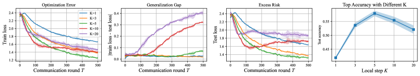
(a) Using same $\eta_{g}$, large local update steps $K$ make FL early over-fitting.

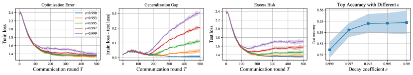
(b) Stabilizing federated optimization ($K=10$) with global learning rate decay $\eta_{g}^{t}=\eta_{g}\cdot\varepsilon^{t}$.

Figure 2: Proof-of-concept experiments on Federated CIFAR10 with Dirichlet partition 0.1.

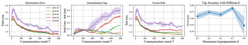
Figure 3: Evaluation of FOSM: large momentum $\beta$ enlarges generalization gap, indicating worsen stability.

Experiments Evaluation

In this section, we conduct proof-of-concept experiments to validate our theory, providing a better understanding of FL practices. Please note that our experiments are to evaluate our theories instead of pursuing SOTA accuracy.

Setup

Our experiment setup follows previous works (McMahan et al. 2017; Wang et al. 2020; Zeng et al. 2023b; Sun, Shen, and Tao 2024). We train neural networks on federated partitioned CIFAR-10/100 datasets (Krizhevsky 2009). We generate the datasets of 100 clients following the latent Dirichlet allocation over labels (Hsu, Qi, and Brown 2019), controlled by a coefficient $Dir=0.1$. Then, we evaluate our theory with 4-layer CNN from work (McMahan et al. 2017) for the CIFAR-10 task and ResNet-18-GN (Wu and He 2018) for the CIFAR-100 task. We select the local learning rate $\eta_{l}=0.01$ and global learning rate $\eta_{g}=1$ for training hyperparameters. And, we set weight decay as $1e^{-3}$ for the local SGD optimizer. We fix the partial participation ratio of 0.1, the total communication round $T=500$. the local batch size $b=32$ and local SGD steps $K=\{1,3,5,10,20\}$. We run all experiments independently with 3 different random seeds and report the mean and standard deviation of results. Due to page limitations, we provide missing experiments in Appendix F.

Observing model fitting status under different $K$

In Figure 2(a), we observe that the $K=5$ case is close to benign-fitting at $T=500$ as the test loss converged. And, the $K=1,3$ case is under-fitting before $T=500$. Curve $K=10$ starts over-fitting after 100 rounds and curve $K=20$ starts over-fitting even earlier. Therefore, when the learning rate is fixed, the local update step should be carefully tuned in practice. Moreover, the training loss curves of $K=\{1,3,5\}$ decrease at a rate proportional to the $K$ which matches its convergence rate. Meanwhile, the test loss decays at a lower speed than the training loss as the excess risk bound is slower.

Generalization gap expands linearly with $K$

Please see the generalization gap plot in Figure 2(a). The generalization gap of the global model increases rapidly at a rate proportional to local update steps $K$. For example, the curve $K=20$ reaches the generalization gap value $0.2$ at communication round $150$ while curve $K=10$ reaches the same point around communication round $300$. It is $2\times$ slower due to the choice of $K$ as shown in Theorem 2.

Empirical optimal $K$ is related to batch size

In Figure 2(a), the excess risk curves and top-accuracy plots show the optimal $K=5$ for the best generalization performance. Moreover, we present the experiment results with batch sizes $b=\{16,64\}$ in Appendix F, which shows that the optimal $K$ is proportional to batch size. For instance, we have the optimal $K=3$ with $b=16$ and optimal $K=10$ with $b=64$. This is because batch size is related to the local stochastic gradient variance $\sigma_{l}^{2}$ and $\sigma_{g}^{2}$.

Improper global learning rate results in early over-fitting

The excess risk dynamics grow fast after a short decrease for training processes $K=\{10,20\}$ in Figure 2(a). We observe unfavorable convergence behavior and over-fitting. As previously discussed, large local update steps $K$ make the stability bounds in Theorem 2 grow too fast. Our theories suggest fixing early over-fitting via global learning rate decay. To validate this point, we re-run the experiment of $K=10$ in Figure 2(b) but additionally decay the global learning rate $\eta_{g}^{t}=\eta_{g}\cdot\varepsilon^{t}$ for $t\in[T]$. We choose decay coefficient $\varepsilon=\{0.999,0.997,0.995,0.993,0.99\}$ with the results shown in Figure 2(b). The results show proper global learning rate decay stabilizes the federated optimization against large steps of local updates.

Large momentum $\beta$ enlarge generalization gap

We report the results of FOSM on the CIFAR-10 task with $K=5$ and $b=32$. This empirical evidence for Theorem 5 is shown in Figure 3. We observe that the training loss curves of FOSM are not very sensitive to low $\beta$. However, the generalization gap is sensitive to the selection of $\beta$. This is because the FOSM model stability expands sub-linearly with $\beta$ (the third term in Theorem 5) from the generalization gap plots. And, we also observed that FOSM typically implements a better test accuracy than Algorithm 1 under the same settings.

Conclusion

This paper proposes an analysis framework for the excess risk bound of federated optimization algorithms. This framework includes a federated global stability analysis framework and trade-off analysis. We prove that jointly optimizing the model stability and optimization trade-off can better describe the excess risk. Importantly, the framework is transferable to arbitrary FL algorithms as shown in the example analysis on FOSM. Experiments evaluate the efficacy of theories and guide future excess risk analysis and FL practices.

Limitation & future work

This paper does not provide any practical approach for enhancing FL algorithms. And, our main theories only show the FL generalization under the clients’ full participation and identical local training setups. It may be interesting for future works to analyze FL settings with partial client participation and heterogeneous local computing. Besides, extending the trade-off analysis into deep learning model training practices (e.g., dropout and weight decay) can be inspiring.

In the appendices, we provide more details and results omitted in the main paper. The appendices are structured as follows:

• Appendix A provides the proof of Theorem 1.

• Appendix B provides the proof of Lemma 1 and Theorem 2 related to model stability analysis.

• Appendix C provides the proof of Theorem 3 related to convergence analysis.

• Appendix D provides the proof of Theorem 4 related to excess risk analysis.

• Appendix E provides the proof of Theorem 5 related to trade-off analysis on FOSM.

• Appendix F elaborates on the experiment details and missing experiment results.

Appendix A: Generalization by On-average Model Stability

Model stability (Lei and Ying 2020) means any perturbation of samples across all clients cannot lead to a big change in the model trained by the algorithm in expectation. It measures the upper bound of algorithm results (final model) differences trained on similar datasets. And, these similar datasets for evaluating stability are called Neighbor datasets (Hardt, Recht, and Singer 2016; Sun, Niu, and Wei 2024):

Definition 2 (Neighbor datasets).

Given a global dataset $\mathcal{D}=\cup_{i=1}^{N}\mathcal{D}_{i}=\{z_{1},\dots,z_{n}\}$, where $\mathcal{D}_{i}$ is the local dataset of the $i$-th client with $|\mathcal{D}_{i}|=n_{i},\forall i\in[N]$. Another global dataset $\tilde{\mathcal{D}}=\cup_{i=1}^{N}\tilde{\mathcal{D}}_{i}=\{\tilde{z}_{1},\dots,\tilde{z}_{n}\}$ be drawn independently from $\mathcal{Z}$ such that $z_{j},\tilde{z}_{j}\sim\mathcal{P}_{i}$ if $z_{j}\in\mathcal{D}_{i}$. For any $j=1,\dots,n$, we define $\mathcal{D}^{(j)}=\{z_{1},\dots,z_{j-1},\tilde{z}_{j},z_{j+1},\dots,z_{n}\}$ is neighboring to $\mathcal{D}$ by replacing the $j$-th element with $\tilde{z}_{j}$.

Then, given a learning algorithm $\mathcal{A}(\cdot)$ and a training dataset $\mathcal{D}$, we denote $\boldsymbol{x}=\mathcal{A}(\mathcal{D})$ as the model generated by the method $\mathcal{A}$ with given data. Then, the upper bound of the model’s generalization gap is established in the following theorem:

Theorem 6 (Modified generalization via model stability).

Let $\mathcal{D},\tilde{\mathcal{D}},\mathcal{D}^{(j)}$ be constructed as Definition 2. Let $\gamma>0$, if for any $z$, the function $f(\boldsymbol{x};z)$ is nonnegative and $L$-smooth, then

$$\mathbb{E}_{\mathcal{D},\mathcal{A}}[F(\mathcal{A}(\mathcal{D}))-f(\mathcal{A}(\mathcal{D}))]\leq\frac{1}{2\gamma}\mathbb{E}_{\mathcal{D},\mathcal{A}}\|\nabla f(\mathcal{A}(\mathcal{D}))\|^{2}+\frac{L+\gamma}{2}\frac{1}{n}\sum_{j=1}^{n}\mathbb{E}_{\mathcal{D},\tilde{\mathcal{D}},\mathcal{A}}[\|\mathcal{A}(\mathcal{D}^{(j)})-\mathcal{A}(\mathcal{D})\|^{2}].$$ (7)

Notation remark: we use $f(\mathcal{A}(\mathcal{D});z)$ to denote the empirical loss of one data sample $z$.

Recalling Definition 2, $\mathcal{D}^{(j)}$ is the neighbor datasets of $\mathcal{D}$ by replacing the $j$-th element $z_{j}$ with $\tilde{z}_{j}$, given the definition of the generalization error, we know

$$\mathbb{E}_{\mathcal{D},\mathcal{A}}[F(\mathcal{A}(\mathcal{D}))-f(\mathcal{A}(\mathcal{D}))] =\mathbb{E}_{\mathcal{D},\mathcal{A}}\Big{[}\frac{1}{n}\sum_{j=1}^{n}\big{(}F(\mathcal{A}(\mathcal{D}))\big{)}\Big{]}-\mathbb{E}_{\mathcal{D},\mathcal{A}}\Big{[}f(\mathcal{A}(\mathcal{D}))\Big{]}$$

$$=\mathbb{E}_{\mathcal{D},\mathcal{A}}\Big{[}\frac{1}{n}\sum_{j=1}^{n}\mathbb{E}_{\tilde{z}_{j}}\big{[}f(\mathcal{A}(\mathcal{D}),\tilde{z}_{j})\big{]}\Big{]}-\mathbb{E}_{\mathcal{D},\mathcal{A}}\Big{[}f(\mathcal{A}(\mathcal{D}))\Big{]}$$

$$=\mathbb{E}_{\mathcal{D},\mathcal{A}}\Big{[}\frac{1}{n}\sum_{j=1}^{n}\mathbb{E}_{\tilde{z}_{j}}\big{[}f(\mathcal{A}(\mathcal{D}),\tilde{z}_{j})\big{]}\Big{]}-\mathbb{E}_{\mathcal{D},\mathcal{A}}\Big{[}\frac{1}{n}\sum_{j=1}^{n}f(\mathcal{A}(\mathcal{D});z_{j})\Big{]}\quad\quad\quad\triangleright\text{Definition of empirical loss}$$

$$=\mathbb{E}_{\mathcal{D},\mathcal{A}}\Big{[}\frac{1}{n}\sum_{j=1}^{n}\mathbb{E}_{\tilde{\mathcal{D}}}\big{[}f(\mathcal{A}(\mathcal{D}),\tilde{z}_{j})\big{]}\Big{]}-\frac{1}{n}\sum_{j=1}^{n}\mathbb{E}_{\mathcal{D},\tilde{\mathcal{D}},\mathcal{A}}\Big{[}f(\mathcal{A}(\mathcal{D}^{(j)});\tilde{z}_{j}))\Big{]}$$

$$=\mathbb{E}_{\mathcal{D},\tilde{\mathcal{D}},\mathcal{A}}\Big{[}\frac{1}{n}\sum_{j=1}^{n}\big{(}f(\mathcal{A}(\mathcal{D}),\tilde{z}_{j})-f(\mathcal{A}(\mathcal{D}^{(j)});\tilde{z}_{j})\big{)}\Big{]}.$$

Recall that we assume the loss function $f(x;z)$ satisfies $L$-smooth, i.e., $\forall\boldsymbol{x},\boldsymbol{y}\in\mathcal{X},\forall z\in\mathcal{Z},\|\nabla f(\boldsymbol{x};z)-\nabla f(\boldsymbol{y};z)\|\leq L\|\boldsymbol{x}-\boldsymbol{y}\|$. Noting that the empirical risk $f(\boldsymbol{x})=\frac{1}{n}\sum_{j=1}^{n}f(\boldsymbol{x};z_{j})$ also satisfies $L$-smooth because $\|\nabla f(\boldsymbol{x})-\nabla f(\boldsymbol{y})\|=\|\frac{1}{n}\sum_{j=1}^{n}\nabla f(\boldsymbol{x};z_{j})-\frac{1}{n}\sum_{j=1}^{n}\nabla f(\boldsymbol{y};z_{j})\|\leq\frac{1}{n}\sum_{j=1}^{n}\|\nabla f(\boldsymbol{x};z_{j})-\nabla f(\boldsymbol{y};z_{j})\|\leq L\|\boldsymbol{x}-\boldsymbol{y}\|$. Based on this finding, we further have

$$\mathbb{E}_{\mathcal{D},\mathcal{A}}[F(\mathcal{A}(\mathcal{D}))-f(\mathcal{A}(\mathcal{D}))]\leq\mathbb{E}_{\mathcal{D},\tilde{\mathcal{D}},\mathcal{A}}\left[\left\langle\mathcal{A}(\mathcal{D}^{(j)})-\mathcal{A}(\mathcal{D}),\frac{1}{n}\sum_{j=1}^{n}\nabla f(\mathcal{A}(\mathcal{D});\tilde{z}_{j})\right\rangle+\frac{L}{2}\left\|\mathcal{A}(\mathcal{D}^{(j)})-\mathcal{A}(\mathcal{D})\right\|^{2}\right].$$

Using Cauchy’s inequality, we have

$$\mathbb{E}_{\mathcal{D},\tilde{\mathcal{D}},\mathcal{A}}\Big{[}\langle\mathcal{A}(\mathcal{D}^{(j)})-\mathcal{A}(\mathcal{D}),\frac{1}{n}\sum_{j=1}^{n}\nabla f(\mathcal{A}(\mathcal{D});\tilde{z}_{j})\rangle\Big{]} \leq\mathbb{E}_{\mathcal{D},\tilde{\mathcal{D}},\mathcal{A}}\Big{[}\|\mathcal{A}(\mathcal{D}^{(j)})-\mathcal{A}(\mathcal{D})\|\cdot\|\nabla f(\mathcal{A}(\mathcal{D}))\|\Big{]}$$

$$\leq\frac{\gamma}{2}\mathbb{E}_{\mathcal{D},\tilde{\mathcal{D}},\mathcal{A}}\|\mathcal{A}(\mathcal{D}^{(j)})-\mathcal{A}(\mathcal{D})\|^{2}+\frac{1}{2\gamma}\mathbb{E}_{\mathcal{D},\tilde{\mathcal{D}},\mathcal{A}}\|\nabla f(\mathcal{A}(\mathcal{D}))\|^{2}.$$

Then, we let the expectation absorb the uniform randomness of samples to simplify the equation:

$$\mathbb{E}_{\mathcal{D},\mathcal{A}}[F(\mathcal{A}(\mathcal{D}))-f(\mathcal{A}(\mathcal{D}))]\leq\frac{L+\gamma}{2}\underbrace{\frac{1}{n}\sum_{j=1}^{n}\mathbb{E}_{\mathcal{D},\tilde{\mathcal{D}},\mathcal{A}}[\|\mathcal{A}(\mathcal{D}^{(j)})-\mathcal{A}(\mathcal{D})\|^{2}]}_{\text{On-average Model stability}}+\frac{1}{2\gamma}\underbrace{\mathbb{E}_{\mathcal{D},\mathcal{A}}\|\nabla f(\mathcal{A}(\mathcal{D}))\|^{2}}_{\text{Gradient norm}},$$

where $\gamma>0$. In the main paper, we simplified some notations such as $\boldsymbol{x}=\mathcal{A}(\mathcal{D})$.

Appendix B: Model Stability Analysis

Proofs of Local Stability

Lemma 2 (Local stability with pertubed sample).

Letting non-negative objectives $f_{i},\forall i\in[N]$ satisfies $L$-smooth and Assumptions 1 2. We suppose the $i$-th client preserves dataset $\mathcal{D}_{i}$ and $|\mathcal{D}_{i}|=n_{i}$ samples. Its neighbor dataset $\mathcal{D}_{i}^{(j)}$ has the perturbed sample $\tilde{z}_{j}\in\mathcal{D}_{i}$ with probability 1. If the $i$-th client conducts $K$ mini-batch SGD steps with batch-size $b$, and non-increasing learning rate $\eta_{l}=\Theta(\frac{1}{KL})$, we prove the stability of local iteration on the $i$-th client for $t\in[T]$ as

$$\mathbb{E}\|\boldsymbol{x}_{i}^{t,K}-\tilde{\boldsymbol{x}}_{i}^{t,K}\|^{2}\leq\phi\underbrace{\mathbb{E}\|\boldsymbol{x}^{t}-\tilde{\boldsymbol{x}}^{t}\|^{2}}_{\text{Global model stability}}+\frac{K}{L^{2}}(\sigma_{l}^{2}+\frac{3b\sigma_{g}^{2}}{n_{i}}),$$

where $\phi=(1+4\eta_{l}L)^{K}>1$ is constant due to $\eta_{l}=\Theta(\frac{1}{KL})$.

Proof of Lemma 2

We investigate the local mini-batch SGD stability on the $i$-th clients with batch size $b_{i}$. $\mathcal{D}_{i}$ is the local datasets and $\mathcal{D}_{i}^{\prime}$ is the neighbor dataset generated analogous to Definition 2. Datasets $\mathcal{D}_{i}$ and $\mathcal{D}_{i}^{\prime}$ differ at most one data sample.

There are two cases to consider in local training.

In the first case, local mini-batch SGD selects non-perturbed samples in $\mathcal{D}_{i}$ and $\mathcal{D}_{i}^{\prime}$. Hence, we have

$$\quad\mathbb{E}\|\boldsymbol{x}_{i}^{t,k+1}-\tilde{\boldsymbol{x}}_{i}^{t,k+1}\|^{2}$$

$$\leq\mathbb{E}\|\boldsymbol{x}_{i}^{t,k}-\tilde{\boldsymbol{x}}_{i}^{t,k}-\eta_{l}(\boldsymbol{g}_{i}^{t,k}-\tilde{\boldsymbol{g}}_{i}^{t,k})\|^{2}$$

$$\leq\mathbb{E}\left[\|\boldsymbol{x}_{i}^{t,k}-\tilde{\boldsymbol{x}}_{i}^{t,k}\|^{2}+\eta_{l}^{2}\|\boldsymbol{g}_{i}^{t,k}-\tilde{\boldsymbol{g}}_{i}^{t,k}\|^{2}-2\eta_{l}\langle\boldsymbol{x}_{i}^{t,k}-\tilde{\boldsymbol{x}}_{i}^{t,k},\boldsymbol{g}_{i}^{t,k}-\tilde{\boldsymbol{g}}_{i}^{t,k}\rangle\right]$$

$$\leq\mathbb{E}\left[\|\boldsymbol{x}_{i}^{t,k}-\tilde{\boldsymbol{x}}_{i}^{t,k}\|^{2}+\eta_{l}^{2}\|\boldsymbol{g}_{i}^{t,k}-\tilde{\boldsymbol{g}}_{i}^{t,k}\|^{2}-2\eta_{l}\langle\boldsymbol{x}_{i}^{t,k}-\tilde{\boldsymbol{x}}_{i}^{t,k},\nabla f_{i}(\boldsymbol{x}_{i}^{t,k})-\nabla f_{i}(\tilde{\boldsymbol{x}}_{i}^{t,k})\rangle\right]$$

$$\leq\mathbb{E}\left[\|\boldsymbol{x}_{i}^{t,k}-\tilde{\boldsymbol{x}}_{i}^{t,k}\|^{2}+\eta_{l}^{2}\|\boldsymbol{g}_{i}^{t,k}-\tilde{\boldsymbol{g}}_{i}^{t,k}\|^{2}+2\eta_{l}L\|\boldsymbol{x}_{i}^{t,k}-\tilde{\boldsymbol{x}}_{i}^{t,k}\|^{2}\right]$$

$$\leq(1+2\eta_{l}L)\mathbb{E}\|\boldsymbol{x}_{i}^{t,k}-\tilde{\boldsymbol{x}}_{i}^{t,k}\|^{2}+\eta_{l}^{2}\mathbb{E}\|\boldsymbol{g}_{i}^{t,k}-\tilde{\boldsymbol{g}}_{i}^{t,k}\|^{2}$$

$$=(1+2\eta_{l}L)\mathbb{E}\|\boldsymbol{x}_{i}^{t,k}-\tilde{\boldsymbol{x}}_{i}^{t,k}\|^{2}+\eta_{l}^{2}\mathbb{E}\|\boldsymbol{g}_{i}^{t,k}\pm\nabla f_{i}(\boldsymbol{x}_{i}^{t,k})-\tilde{\boldsymbol{g}}_{i}^{t,k}\pm\nabla f_{i}(\tilde{\boldsymbol{x}}_{i}^{t,k})\|^{2}$$

$$\leq(1+2\eta_{l}L)\mathbb{E}\|\boldsymbol{x}_{i}^{t,k}-\tilde{\boldsymbol{x}}_{i}^{t,k}\|^{2}+2\eta_{l}^{2}\mathbb{E}\|\boldsymbol{g}_{i}^{t,k}-\nabla f_{i}(\boldsymbol{x}_{i}^{t,k})-\tilde{\boldsymbol{g}}_{i}^{t,k}+\nabla f_{i}(\tilde{\boldsymbol{x}}_{i}^{t,k})\|^{2}+2\eta_{l}^{2}\mathbb{E}\|\nabla f_{i}(\boldsymbol{x}_{i}^{t,k})-\nabla f_{i}(\tilde{\boldsymbol{x}}_{i}^{t,k})\|^{2}$$

$$\leq(1+2\eta_{l}L)\mathbb{E}\|\boldsymbol{x}_{i}^{t,k}-\tilde{\boldsymbol{x}}_{i}^{t,k}\|^{2}+2\eta_{l}^{2}\mathbb{E}\|\boldsymbol{g}_{i}^{t,k}-\nabla f_{i}(\boldsymbol{x}_{i}^{t,k})\|^{2}+2\eta_{l}^{2}\mathbb{E}\|\tilde{\boldsymbol{g}}_{i}^{t,k}-\nabla f_{i}(\tilde{\boldsymbol{x}}_{i}^{t,k})\|^{2}+2\eta_{l}^{2}\mathbb{E}\|\nabla f_{i}(\boldsymbol{x}_{i}^{t,k})-\nabla f_{i}(\tilde{\boldsymbol{x}}_{i}^{t,k})\|^{2}$$

$$\leq(1+2\eta_{l}L+2\eta_{l}^{2}L^{2})\mathbb{E}\|\boldsymbol{x}_{i}^{t,k}-\tilde{\boldsymbol{x}}_{i}^{t,k}\|^{2}+4\eta_{l}^{2}\sigma_{l}^{2}.$$

In the second case, local mini-batch SGD samples a batch data that involves the perturbed sample $\tilde{z}$ from $\mathcal{D}_{i}$ and $\mathcal{D}_{i}^{\prime}$, which happens with probability $b_{i}/n_{i}$. Analogously, we have

$$\quad\mathbb{E}\|\boldsymbol{x}_{i}^{t,k+1}-\tilde{\boldsymbol{x}}_{i}^{t,k+1}\|^{2}$$ (8)

$$\leq\mathbb{E}\|\boldsymbol{x}_{i}^{t,k}-\tilde{\boldsymbol{x}}_{i}^{t,k}-\eta_{l}(\boldsymbol{g}_{i}^{t,k}-\tilde{\boldsymbol{g}}_{i}^{t,k})\|^{2}$$

$$\leq\mathbb{E}\left[\|\boldsymbol{x}_{i}^{t,k}-\tilde{\boldsymbol{x}}_{i}^{t,k}\|^{2}+\eta_{l}^{2}\|\boldsymbol{g}_{i}^{t,k}-\tilde{\boldsymbol{g}}_{i}^{t,k}\|^{2}-2\eta_{l}\langle\boldsymbol{x}_{i}^{t,k}-\tilde{\boldsymbol{x}}_{i}^{t,k},\boldsymbol{g}_{i}^{t,k}-\tilde{\boldsymbol{g}}_{i}^{t,k}\rangle\right]$$

$$\leq\mathbb{E}\left[\|\boldsymbol{x}_{i}^{t,k}-\tilde{\boldsymbol{x}}_{i}^{t,k}\|^{2}+\eta_{l}^{2}\|\boldsymbol{g}_{i}^{t,k}-\tilde{\boldsymbol{g}}_{i}^{t,k}\|^{2}-2\eta_{l}\langle\boldsymbol{x}_{i}^{t,k}-\tilde{\boldsymbol{x}}_{i}^{t,k},\nabla f_{i}(\boldsymbol{x}_{i}^{t,k})-\nabla f_{i}(\tilde{\boldsymbol{x}}_{i}^{t,k})\rangle\right]$$

$$\leq\mathbb{E}\left[\|\boldsymbol{x}_{i}^{t,k}-\tilde{\boldsymbol{x}}_{i}^{t,k}\|^{2}+\eta_{l}^{2}\|\boldsymbol{g}_{i}^{t,k}-\tilde{\boldsymbol{g}}_{i}^{t,k}\|^{2}+2\eta_{l}L\|\boldsymbol{x}_{i}^{t,k}-\tilde{\boldsymbol{x}}_{i}^{t,k}\|^{2}\right]$$

$$\leq(1+2\eta_{l}L)\mathbb{E}\|\boldsymbol{x}_{i}^{t,k}-\tilde{\boldsymbol{x}}_{i}^{t,k}\|^{2}+\eta_{l}^{2}\mathbb{E}\|\boldsymbol{g}_{i}^{t,k}-\tilde{\boldsymbol{g}}_{i}^{t,k}\|^{2}$$

$$\leq(1+2\eta_{l}L)\mathbb{E}\|\boldsymbol{x}_{i}^{t,k}-\tilde{\boldsymbol{x}}_{i}^{t,k}\|^{2}+\eta_{l}^{2}\mathbb{E}\|\boldsymbol{g}_{i}^{t,k}\pm\nabla f_{i}(\boldsymbol{x}_{i}^{t,k};z)-\tilde{\boldsymbol{g}}_{i}^{t,k}\pm\nabla f_{i}(\tilde{\boldsymbol{x}}_{i}^{t,k};\tilde{z})\|^{2}$$

$$\leq(1+2\eta_{l}L)\mathbb{E}\|\boldsymbol{x}_{i}^{t,k}-\tilde{\boldsymbol{x}}_{i}^{t,k}\|^{2}+4\eta_{l}^{2}\sigma_{l}^{2}+2\eta_{l}^{2}\mathbb{E}\|\nabla f_{i}(\boldsymbol{x}_{i}^{t,k};z)-\nabla f_{i}(\tilde{\boldsymbol{x}}_{i}^{t,k};\tilde{z})\|^{2}$$

$$\leq(1+2\eta_{l}L)\mathbb{E}\|\boldsymbol{x}_{i}^{t,k}-\tilde{\boldsymbol{x}}_{i}^{t,k}\|^{2}+4\eta_{l}^{2}\sigma_{l}^{2}+2\eta_{l}^{2}\mathbb{E}\|\nabla f_{i}(\boldsymbol{x}_{i}^{t,k};z)\pm\nabla f(\boldsymbol{x}_{i}^{t,k})-\nabla f_{i}(\tilde{\boldsymbol{x}}_{i}^{t,k};\tilde{z})\pm\nabla f(\tilde{\boldsymbol{x}}_{i}^{t,k})\|^{2}$$

$$\leq(1+2\eta_{l}L)\mathbb{E}\|\boldsymbol{x}_{i}^{t,k}-\tilde{\boldsymbol{x}}_{i}^{t,k}\|^{2}+4\eta_{l}^{2}\sigma_{l}^{2}$$

$$\quad+2\eta_{l}^{2}\mathbb{E}\|(\nabla f_{i}(\boldsymbol{x}_{i}^{t,k};z)-\nabla f(\boldsymbol{x}_{i}^{t,k}))-(\nabla f_{i}(\tilde{\boldsymbol{x}}_{i}^{t,k};\tilde{z})-\nabla f(\tilde{\boldsymbol{x}}_{i}^{t,k}))+(\nabla f(\boldsymbol{x}_{i}^{t,k}))-\nabla f(\tilde{\boldsymbol{x}}_{i}^{t,k})))\|^{2}$$

$$\leq(1+2\eta_{l}L)\mathbb{E}\|\boldsymbol{x}_{i}^{t,k}-\tilde{\boldsymbol{x}}_{i}^{t,k}\|^{2}+4\eta_{l}^{2}\sigma_{l}^{2}+12\eta_{l}^{2}\sigma_{g}^{2}+6\eta_{l}^{2}\mathbb{E}\|\boldsymbol{x}_{i}^{t,k}-\tilde{\boldsymbol{x}}_{i}^{t,k}\|^{2}\quad\quad\quad\triangleright\text{Assumption~{}\ref{asp:bgv}}$$

$$\leq(1+2\eta_{l}L+6\eta_{l}^{2}L^{2})\mathbb{E}\|\boldsymbol{x}_{i}^{t,k}-\tilde{\boldsymbol{x}}_{i}^{t,k}\|^{2}+4\eta_{l}^{2}(\sigma_{l}^{2}+3\sigma_{g}^{2})$$

Bounding local uniform Stability. Now, we can combine these two cases. Our bound relies on the probability of whether the perturbed samples are involved. We use $\xi$ to denote the random batch in local training. Thus, we have:

$$\quad\mathbb{E}_{\mathcal{D}_{i},\mathcal{D}_{i}^{\prime}}\|\boldsymbol{x}_{i}^{t,k+1}-\tilde{\boldsymbol{x}}_{i}^{t,k+1}\|^{2}$$

$$\leq P(\tilde{z}\notin\xi)\mathbb{E}[\|\boldsymbol{x}_{i}^{t,k+1}-\tilde{\boldsymbol{x}}_{i}^{t,k+1}\|^{2}|\tilde{z}\notin\xi]+P(\tilde{z}\in\xi)\mathbb{E}[\|\boldsymbol{x}_{i}^{t,k+1}-\tilde{\boldsymbol{x}}_{i}^{t,k+1}\|^{2}|\tilde{z}\in\xi]$$

$$\leq(1-\frac{b_{i}}{n_{i}})\big{(}(1+2\eta_{l}L+2\eta_{l}^{2}L^{2})\mathbb{E}\|\boldsymbol{x}_{i}^{t,k}-\tilde{\boldsymbol{x}}_{i}^{t,k}\|^{2}+4\eta_{l}^{2}\sigma_{l}^{2}\big{)}+\frac{b_{i}}{n_{i}}\big{(}(1+2\eta_{l}L+6\eta_{l}^{2}L^{2})\mathbb{E}\|\boldsymbol{x}_{i}^{t,k}-\tilde{\boldsymbol{x}}_{i}^{t,k}\|^{2}+4\eta_{l}^{2}(\sigma_{l}^{2}+3\sigma_{g}^{2})\big{)}$$

$$=(1+2\eta_{l}L+2(1+2b_{i}/n_{i})\eta_{l}^{2}L^{2})\mathbb{E}\|\boldsymbol{x}_{i}^{t,k}-\tilde{\boldsymbol{x}}_{i}^{t,k}\|^{2}+4\eta_{l}^{2}(\sigma_{l}^{2}+\frac{3b_{i}\sigma_{g}^{2}}{n_{i}})\quad\quad\quad\triangleright\text{$b_{i}/n_{i}\leq 1/2$}$$

$$\leq(1+2\eta_{l}L+4\eta_{l}^{2}L^{2})\mathbb{E}\|\boldsymbol{x}_{i}^{t,k}-\tilde{\boldsymbol{x}}_{i}^{t,k}\|^{2}+4\eta_{l}^{2}(\sigma_{l}^{2}+\frac{3b_{i}\sigma_{g}^{2}}{n_{i}})\quad\quad\quad\triangleright\text{$1+2\eta_{l}L\leq 2$}$$

$$\leq(1+4\eta_{l}L)\mathbb{E}\|\boldsymbol{x}_{i}^{t,k}-\tilde{\boldsymbol{x}}_{i}^{t,k}\|^{2}+\frac{1}{L^{2}}(\sigma_{l}^{2}+\frac{3b_{i}\sigma_{g}^{2}}{n_{i}}),$$

where $\xi$ denotes a mini-batch data sampled from the local dataset.

According to the FL protocol, we know $\boldsymbol{x}^{t}=\boldsymbol{x}^{t,0},\tilde{\boldsymbol{x}}^{t}=\tilde{\boldsymbol{x}}^{t,0}$. Then, we unroll the above equation over local steps from $K_{i}$ down to $k=1$ ($K_{i}>1$):

$$\mathbb{E}_{\mathcal{D}_{i},\mathcal{D}_{i}^{\prime}}\|\boldsymbol{x}_{i}^{t,K}-\tilde{\boldsymbol{x}}_{i}^{t,K}\|^{2} \leq\prod_{\tau=k}^{K_{i}-1}(1+4\eta_{l}L)\mathbb{E}\|\boldsymbol{x}_{i}^{t,0}-\tilde{\boldsymbol{x}}_{i}^{t,0}\|^{2}+\sum_{k=1}^{K_{i}-1}\prod_{\tau=k}^{K_{i}-1}(1+4\eta_{l}L)^{\tau}\frac{1}{L^{2}}(\sigma_{l}^{2}+\frac{3b_{i}\sigma_{g}^{2}}{n_{i}})$$

$$\leq(1+4\eta_{l}L)^{K_{i}}\mathbb{E}\|\boldsymbol{x}^{t}-\tilde{\boldsymbol{x}}^{t}\|^{2}+\frac{1}{L^{2}}(\sigma_{l}^{2}+\frac{3b_{i}\sigma_{g}^{2}}{n_{i}})\frac{(1+4\eta_{l}L)^{K_{i}}-1}{4\eta_{l}L}.$$

Here, if we set local learning rate $\eta_{l}=\Theta(\frac{1}{KL})$, we have $(1+4\eta_{l}L)^{K_{i}}-1=\Theta(1)$ and know

$$\mathbb{E}_{\mathcal{D}_{i},\mathcal{D}_{i}^{\prime}}\|\boldsymbol{x}_{i}^{t,K}-\tilde{\boldsymbol{x}}_{i}^{t,K}\|^{2}\leq(1+4\eta_{l}L)^{K_{i}}\mathbb{E}\|\boldsymbol{x}^{t}-\tilde{\boldsymbol{x}}^{t}\|^{2}+\frac{K_{i}}{L^{2}}(\sigma_{l}^{2}+\frac{3b_{i}\sigma_{g}^{2}}{n_{i}}).$$ (9)

For simple equations, we can further use the fact that $(1+\frac{1}{4K})^{K}\leq 2$ to have

$$\mathbb{E}_{\mathcal{D}_{i},\mathcal{D}_{i}^{\prime}}\|\boldsymbol{x}_{i}^{t,K}-\tilde{\boldsymbol{x}}_{i}^{t,K}\|^{2}\leq 2\mathbb{E}\|\boldsymbol{x}^{t}-\tilde{\boldsymbol{x}}^{t}\|^{2}+\frac{K_{i}}{L^{2}}(\sigma_{l}^{2}+\frac{3b_{i}\sigma_{g}^{2}}{n_{i}}).$$ (10)

The proof is complete.

Corollary 2 (Local stability observed by FL server).

Lemma 2 proves the expectation of local expansion with a perturbed sample. Importantly, the local stability of local updates is conditioned by the uniform stability over the whole FL system. Therefore, we need to consider further the probability $P(\tilde{z}\in\mathcal{D}_{i}),\forall i\in[N]$. Intuitively, the $i$-th local dataset $\mathcal{D}_{i}$ and $\tilde{D}_{i}$ differ with one perturbed sample is proportional to the size of local datasets, i.e., $P(\tilde{z}\in\mathcal{D}_{i})=n_{i}/n,\forall i\in[N]$. Then, we have the bounded gap of local updates on the $i$-th client:

$$\mathbb{E}\|\tilde{\boldsymbol{d}}_{i}^{t}-\boldsymbol{d}_{i}^{t}\|^{2}\leq((1+p)+(1+4\eta_{l}L)^{K_{i}})\mathbb{E}\|\boldsymbol{x}^{t}-\tilde{\boldsymbol{x}}^{t}\|^{2}+(1+p^{-1})\frac{K_{i}}{L^{2}}(\sigma_{l}^{2}+\frac{3b_{i}\sigma_{g}^{2}}{n}).$$ (11)

Proof.

We investigate the bound starting with the definition:

$$\mathbb{E}\|\tilde{\boldsymbol{d}}_{i}^{t}-\boldsymbol{d}_{i}^{t}\|^{2} =\mathbb{E}\|(\tilde{\boldsymbol{x}}_{i}^{t,K_{i}}-\tilde{\boldsymbol{x}}^{t})-(\boldsymbol{x}_{i}^{t,K_{i}}-\boldsymbol{x}^{t})\|^{2}$$

$$\leq(1+p)\mathbb{E}\|\boldsymbol{x}^{t}-\tilde{\boldsymbol{x}}^{t}\|^{2}+(1+p^{-1})\mathbb{E}\|\tilde{\boldsymbol{x}}_{i}^{t,K_{i}}-\boldsymbol{x}_{i}^{t,K_{i}}\|^{2}$$

$$\leq(1+p)\mathbb{E}\|\boldsymbol{x}^{t}-\tilde{\boldsymbol{x}}^{t}\|+(1+p^{-1})\mathcal{P}(\tilde{z}\in\mathcal{D}_{i})\mathbb{E}\left[\|\tilde{\boldsymbol{x}}_{i}^{t,K_{i}}-\boldsymbol{x}_{i}^{t,K_{i}}\||\tilde{z}\in\mathcal{D}_{i}\right]$$

$$\quad+(1+p^{-1})\mathcal{P}(\tilde{z}\notin\mathcal{D}_{i})\mathbb{E}_{\mathcal{D}_{i}}\left[\|\tilde{\boldsymbol{x}}_{i}^{t,K_{i}}-\boldsymbol{x}_{i}^{t,K_{i}}\||\tilde{z}\notin\mathcal{D}_{i}\right]$$

$$\leq(1+p)\mathbb{E}\|\boldsymbol{x}^{t}-\tilde{\boldsymbol{x}}^{t}\|+(1+p^{-1})\frac{n_{i}}{n}\underbrace{\mathbb{E}\left[\|\tilde{\boldsymbol{x}}_{i}^{t,K_{i}}-\boldsymbol{x}_{i}^{t,K_{i}}\||\tilde{z}\in\mathcal{D}_{i}\right]}_{\eqref{app:eq_local_datability}}+(1+p^{-1})\frac{n-n_{i}}{n}\underbrace{\mathbb{E}\left[\|\tilde{\boldsymbol{x}}_{i}^{t,K_{i}}-\boldsymbol{x}_{i}^{t,K_{i}}\||\tilde{z}\notin\mathcal{D}_{i}\right]}_{\text{Given below}}.$$

Then, we let $b_{i}=0$ for (9) denote the local stability without the perturbed sample (i.e., $\tilde{z}\notin\mathcal{D}_{i}$). In this case, the local mini-batch SGD updates are expansive due to local gradient variance and multi-steps as:

$$\mathbb{E}_{\mathcal{D}_{i}}\|\boldsymbol{x}_{i}^{t,K_{i}}-\tilde{\boldsymbol{x}}_{i}^{t,K_{i}}\|^{2}\leq(1+4\eta_{l}L)^{K_{i}}\mathbb{E}\|\boldsymbol{x}^{t}-\tilde{\boldsymbol{x}}^{t}\|^{2}+\frac{K_{i}}{L^{2}}\sigma_{l}^{2}$$

Combining all results, we have

$$\mathbb{E}\|\tilde{\boldsymbol{d}}_{i}^{t}-\boldsymbol{d}_{i}^{t}\|^{2}\leq((1+p)+(1+4\eta_{l}L)^{K_{i}})\mathbb{E}\|\boldsymbol{x}^{t}-\tilde{\boldsymbol{x}}^{t}\|^{2}+(1+p^{-1})\frac{K_{i}}{L^{2}}(\sigma_{l}^{2}+\frac{3b_{i}\sigma_{g}^{2}}{n}),$$

and conclude the results.

Proofs of Global Stability (Lemma 1 and Theorem 2)

Proof of Lemma 1

We now prove the global stability of global update rules. Using the standard inequality $(a+b)^{2}\leq(1+p)a^{2}+(1+p^{-1})b^{2}$, we know

$$\mathbb{E}\|\boldsymbol{x}^{t+1}-\tilde{\boldsymbol{x}}^{t+1}\|^{2} =\mathbb{E}\|\boldsymbol{x}^{t}-\eta_{g}\boldsymbol{d}^{t}-\tilde{\boldsymbol{x}}^{t}+\eta_{g}\tilde{\boldsymbol{d}}^{t}\|^{2}$$ (12)

$$=\mathbb{E}\|(\boldsymbol{x}^{t}-\tilde{\boldsymbol{x}}^{t})-\eta_{g}(\boldsymbol{d}^{t}-\tilde{\boldsymbol{d}}^{t})\|^{2}$$

$$\leq(1+p)\mathbb{E}\|\boldsymbol{x}^{t}-\tilde{\boldsymbol{x}}^{t}\|^{2}+(1+p^{-1})\eta_{g}^{2}\mathbb{E}\|\boldsymbol{d}^{t}-\tilde{\boldsymbol{d}}^{t}\|^{2}$$

$$\leq(1+p)\mathbb{E}\|\boldsymbol{x}^{t}-\tilde{\boldsymbol{x}}^{t}\|^{2}+(1+p^{-1})\eta_{g}^{2}\mathbb{E}\|\frac{1}{N}\sum_{i=1}^{N}(\boldsymbol{d}_{i}^{t}-\tilde{\boldsymbol{d}}_{i}^{t})\|^{2}$$

$$\leq(1+p)\mathbb{E}\|\boldsymbol{x}^{t}-\tilde{\boldsymbol{x}}^{t}\|^{2}+(1+p^{-1})\frac{\eta_{g}^{2}}{N^{2}}\mathbb{E}\|\sum_{i=1}^{N}(\boldsymbol{d}_{i}^{t}-\tilde{\boldsymbol{d}}_{i}^{t})\|^{2}$$

$$\leq(1+p)\mathbb{E}\|\boldsymbol{x}^{t}-\tilde{\boldsymbol{x}}^{t}\|^{2}+(1+p^{-1})\frac{\eta_{g}^{2}}{N}\sum_{i=1}^{N}\mathbb{E}\|\boldsymbol{d}_{i}^{t}-\tilde{\boldsymbol{d}}_{i}^{t}\|^{2}$$

If the local SGD of all clients uses the same setting $K=K_{i},b=b_{i},\forall i$, we have the global stability:

$$\mathbb{E}\|\boldsymbol{x}^{t+1}-\tilde{\boldsymbol{x}}^{t+1}\|^{2} \leq(1+p)\mathbb{E}\|\boldsymbol{x}^{t}-\tilde{\boldsymbol{x}}^{t}\|^{2}$$

$$\quad+(1+p^{-1})\eta_{g}^{2}\left(((1+p)+(1+4\eta_{l}L)^{K})\mathbb{E}\|\boldsymbol{x}^{t}-\tilde{\boldsymbol{x}}^{t}\|^{2}+(1+p^{-1})\frac{K}{L^{2}}(\sigma_{l}^{2}+\frac{3b\sigma_{g}^{2}}{n})\right)$$

$$\leq(1+p)\left(1+p^{-1}((1+p)+(1+4\eta_{l}L)^{K})\eta_{g}^{2}\right)\mathbb{E}\|\boldsymbol{x}^{t}-\tilde{\boldsymbol{x}}^{t}\|^{2}+(1+p^{-1})^{2}\frac{K}{L^{2}}(\sigma_{l}^{2}+\frac{3b\sigma_{g}^{2}}{n})\eta_{g}^{2}.$$

Letting $\psi_{1}=p^{-1}((1+p)+(1+4\eta_{l}L)^{K}),\psi_{2}=\frac{K}{L^{2}}(\sigma_{l}^{2}+\frac{3b\sigma_{g}^{2}}{n})$, it yields that

$$\mathbb{E}\|\boldsymbol{x}^{t+1}-\tilde{\boldsymbol{x}}^{t+1}\|^{2}\leq(1+p)(1+\psi_{1}\eta_{g}^{2})\mathbb{E}\|\boldsymbol{x}^{t}-\tilde{\boldsymbol{x}}^{t}\|^{2}+(1+p^{-1})^{2}\psi_{2}\eta_{g}^{2},$$ (13)

which concludes the expansion of global stability.

Proof of Theorem 2

We let the global learning rate $\eta_{g}$ subjected to time $t$ to know

$$\mathbb{E}\|\boldsymbol{x}^{t+1}-\tilde{\boldsymbol{x}}^{t+1}\|^{2}\leq(1+p)(1+\psi_{1}(\eta_{g}^{t})^{2})\mathbb{E}\|\boldsymbol{x}^{t}-\tilde{\boldsymbol{x}}^{t}\|^{2}+(1+p^{-1})^{2}\psi_{2}(\eta_{g}^{t})^{2}.$$ (14)

Then, unrolling the above equation from time $0$ to $t$ and using that $\boldsymbol{x}^{0}=\tilde{\boldsymbol{x}}^{0}$, we get

$$\mathbb{E}\|\boldsymbol{x}^{t+1}-\tilde{\boldsymbol{x}}^{t+1}\|^{2}\leq(1+p^{-1})^{2}\psi_{2}\sum_{\tau=0}^{t}\left((1+p)^{t-\tau+1}\prod_{k=\tau}^{t}\exp\{\psi_{1}(\eta_{g}^{k})^{2}\}\right)(\eta_{g}^{\tau})^{2},$$ (15)

where we use $(1+\psi_{1}(\eta_{g}^{t})^{2})\leq\exp\{\psi_{1}(\eta_{g}^{k})^{2}\}$. Then, we let $(\eta_{g}^{t})^{2}\leq\frac{c}{t}$ to obtain:

$$\mathbb{E}\|\boldsymbol{x}^{t+1}-\tilde{\boldsymbol{x}}^{t+1}\|^{2} \leq(1+p^{-1})^{2}\psi_{2}\sum_{\tau=0}^{t}\left((1+p)^{t-\tau+1}\prod_{k=\tau}^{t}\exp\{c\psi_{1}/k\}\right)\frac{c}{\tau}$$ (16)

$$=(1+p^{-1})^{2}\psi_{2}\sum_{\tau=0}^{t}\left((1+p)^{t-\tau+1}\exp\{c\psi_{1}\sum_{k=\tau}^{t}{\frac{1}{k}}\}\right)\frac{c}{\tau}$$

$$\leq(1+p^{-1})^{2}\psi_{2}\sum_{\tau=0}^{t}\left((1+p)^{t-\tau+1}\exp\{c\psi_{1}\log(\frac{t}{\tau})\}\right)\frac{c}{\tau}$$

$$\leq(1+p^{-1})^{2}(1+p)^{t}\psi_{2}t^{c\psi_{1}}\sum_{\tau=0}^{t}c(\frac{1}{\tau})^{1+c\psi_{1}}\quad\quad\quad\triangleright\text{$\sum_{\tau=0}^{t}(\frac{1}{\tau})^{1+c\psi_{1}}\leq\frac{1}{c\psi_{1}}$}$$

$$\leq(1+p^{-1})^{2}(1+p)^{t}\frac{\psi_{2}}{\psi_{1}}t^{c\psi_{1}}.$$

Then, we let the local learning rate $\eta_{l}=\Theta(\frac{1}{KL})$, we can know that $\psi_{1}=\Theta(1)$ and $\psi_{2}=\Theta(\frac{K}{L^{2}}(\sigma_{l}^{2}+\frac{\sigma_{g}^{2}}{n}))$. Thus, we have

$$\mathbb{E}\|\boldsymbol{x}^{T}-\tilde{\boldsymbol{x}}^{T}\|^{2}\leq\mathcal{O}\left(\frac{K}{L^{2}}(\sigma_{l}^{2}+\frac{\sigma_{g}^{2}}{n})T^{c\psi_{1}}\right),$$ (17)

which concludes the proof.

Appendix C: Convergence Analysis

Here, we prove the convergence rate of the global descent rule:

$$\text{{Client: }}\boldsymbol{d}_{i}^{t}=\boldsymbol{x}_{i}^{t,K}-\boldsymbol{x}_{i}^{t,0}=\eta_{l}\sum_{k=0}^{K-1}\boldsymbol{g}_{i}^{t,k};$$

$$\text{{Server: }}\boldsymbol{x}^{t+1}=\boldsymbol{x}^{t}-\eta_{g}\sum_{i=1}^{N}\boldsymbol{\lambda}_{i}\boldsymbol{d}_{i}^{t}=\boldsymbol{x}^{t}-\eta_{g}\boldsymbol{d}^{t}.$$

Specifically, we analyze the update rule on the server-side gradient descent

$$\boldsymbol{x}^{t+1}=\boldsymbol{x}^{t}-\eta_{g}\boldsymbol{d}^{t}.$$

Without loss of generality, we rewrite the global descent rule as:

$$\boldsymbol{x}^{t+1}=\boldsymbol{x}^{t}-\eta\tilde{\boldsymbol{d}}^{t}=\boldsymbol{x}^{t}-\eta\frac{1}{N}\sum_{i=1}^{N}\frac{\boldsymbol{d}_{i}^{t}}{K}=\boldsymbol{x}^{t}-\frac{\eta}{K}\frac{1}{N}\sum_{i=1}^{N}\sum_{k=1}^{K}\boldsymbol{g}_{i}^{t,k-1},$$

where $\eta=K\eta_{l}\eta_{g}$ and $\tilde{\boldsymbol{d}}^{t}=\boldsymbol{d}^{t}/\eta_{l}K$.

Key Lemmas

Lemma 3 (Bounded local drift(Reddi et al. 2020)).

Let Assumption 1 2 hold. When $\eta_{l}\leq\frac{1}{8KL}$, for any $k\in[K]$, we have

$$\frac{1}{N}\sum_{i=1}^{N}\mathbb{E}\left\|\boldsymbol{x}_{i}^{t,k}-\boldsymbol{x}^{t}\right\|^{2}\leq 5K\eta_{l}^{2}(\sigma_{l}^{2}+6K\sigma_{g}^{2})+30K^{2}\eta_{l}^{2}\mathbb{E}\left\|\nabla f(\boldsymbol{x}^{t})\right\|^{2}$$ (18)

Lemma 4 (Bounded divergence of regularized global updates).

Using $L$-smooth and Assumption 1 2, for all client $i\in[N]$ with local iteration steps $k\in[K]$ and local learning rate $\frac{1}{16KL}\leq\eta_{l}\leq\frac{1}{8KL}$, the differences between uploaded local updates and local first-order gradient can be bounded

$$\mathbb{E}\|\nabla f(\boldsymbol{x}^{t})-\tilde{\boldsymbol{d}}^{t}\|^{2}\leq\frac{15}{16}\mathbb{E}\|\nabla f(\boldsymbol{x}^{t})\|^{2}+60L^{2}\left(9\sigma_{l}^{2}+K\sigma_{g}^{2}\right)K\eta_{l}^{2}.$$ (19)

Proof.

$$\mathbb{E}\|\nabla f(\boldsymbol{x}^{t})-\tilde{\boldsymbol{d}}^{t}\|^{2} =\mathbb{E}\left\|\frac{1}{N}\sum_{i=1}^{N}\nabla f_{i}(\boldsymbol{x}^{t})-\frac{1}{N}\sum_{i=1}^{N}\frac{\boldsymbol{d}_{i}^{t}}{\eta_{l}K}\right\|^{2}\leq\frac{1}{N}\sum_{i=1}^{N}\mathbb{E}\left\|\nabla f_{i}(\boldsymbol{x}^{t})-\frac{\boldsymbol{d}_{i}^{t}}{\eta_{l}K}\right\|^{2}$$

$$=\frac{1}{N}\sum_{i=1}^{N}\mathbb{E}\left\|\frac{1}{K}\sum_{k=1}^{K}\left(\nabla f_{i}(\boldsymbol{x}^{t})\pm\nabla f_{i}(\boldsymbol{x}^{t,k-1})\right)-\frac{\boldsymbol{d}_{i}^{t}}{\eta_{l}K}\right\|^{2}$$

$$\leq 2\frac{1}{N}\sum_{i=1}^{N}\frac{1}{K}\sum_{k=1}^{K}\mathbb{E}\|\nabla f_{i}(\boldsymbol{x}^{t})-\nabla f_{i}(\boldsymbol{x}^{t,k-1})\|^{2}$$

$$\quad+2\mathbb{E}\|\frac{1}{K}\sum_{k=1}^{K}\nabla f_{i}(\boldsymbol{x}^{t,k-1})-\frac{1}{K}\sum_{k=1}^{K}\boldsymbol{g}_{i}^{t,k-1}\|^{2}$$

$$\leq 2\frac{1}{N}\sum_{i=1}^{N}\frac{1}{K}\sum_{k=1}^{K}\mathbb{E}\|\nabla f_{i}(\boldsymbol{x}^{t})-\nabla f_{i}(\boldsymbol{x}^{t,k-1})\|^{2}$$

$$\quad+2\frac{1}{N}\sum_{i=1}^{N}\frac{1}{K^{2}}\sum_{k=1}^{K}\mathbb{E}\|\nabla f_{i}(\boldsymbol{x}^{t,k-1})-\boldsymbol{g}_{i}^{t,k-1}\|^{2}$$

Then, using the L-smoothness of $f$ and unbiasedness of local stochastic gradients, we know

$$\mathbb{E}\|\nabla f(\boldsymbol{x}^{t})-\tilde{\boldsymbol{d}}^{t}\|^{2} \leq 2L^{2}\frac{1}{K}\sum_{k=1}^{K}\frac{1}{N}\sum_{i=1}^{N}\mathbb{E}\|\boldsymbol{x}^{t}-\boldsymbol{x}^{t,k-1}\|^{2}+2\frac{\sigma_{l}^{2}}{K}$$

$$\leq 2L^{2}\left(5K\eta_{l}^{2}(\sigma_{l}^{2}+6K\sigma_{g}^{2})+30K^{2}\eta_{l}^{2}\mathbb{E}\left\|\nabla f(\boldsymbol{x}^{t})\right\|^{2}\right)+2\frac{\sigma_{l}^{2}}{K}$$

$$\leq 60K^{2}L^{2}\eta_{l}^{2}\mathbb{E}\|\nabla f(\boldsymbol{x}^{t})\|^{2}+(10KL^{2}\eta_{l}^{2}+\frac{2}{K})\sigma_{l}^{2}+60K^{2}L^{2}\eta_{l}^{2}\sigma_{g}^{2}.$$

Then, using $\frac{1}{16KL}\leq\eta_{l}\leq\frac{1}{8KL}$, we have

$$\mathbb{E}\|\nabla f(\boldsymbol{x}^{t})-\tilde{\boldsymbol{d}}^{t}\|^{2} \leq\frac{15}{16}\mathbb{E}\|\nabla f(\boldsymbol{x}^{t})\|^{2}+10L^{2}\left((1+\frac{1}{5\eta_{l}^{2}K^{2}L^{2}})\sigma_{l}^{2}+6K\sigma_{g}^{2}\right)K\eta_{l}^{2}$$

$$\leq\frac{15}{16}\mathbb{E}\|\nabla f(\boldsymbol{x}^{t})\|^{2}+60L^{2}\left(9\sigma_{l}^{2}+K\sigma_{g}^{2}\right)K\eta_{l}^{2}.$$

Proof of Descent Lemma

Using the smoothness of $f$ and taking expectations conditioned on $x$, we have

$$\mathbb{E}\left[f(\boldsymbol{x}^{t+1})\right] =\mathbb{E}[f(\boldsymbol{x}^{t}-\eta\tilde{\boldsymbol{d}}^{t})]\leq f(\boldsymbol{x}^{t})-\eta\mathbb{E}[\left\langle\nabla f(\boldsymbol{x}^{t}),\tilde{\boldsymbol{d}}^{t}\right\rangle]+\frac{L}{2}\eta^{2}\mathbb{E}\left[\|\tilde{\boldsymbol{d}}^{t}\|^{2}\right]$$ (20)

$$\leq f(\boldsymbol{x}^{t})-\eta\mathbb{E}[\left\langle\nabla f(\boldsymbol{x}^{t}),\tilde{\boldsymbol{d}}^{t}\right\rangle]+\frac{L}{2}\eta^{2}\mathbb{E}\left[\|\tilde{\boldsymbol{d}}^{t}\|^{2}\right]$$

$$\leq f(\boldsymbol{x}^{t})-\eta\mathbb{E}\|\nabla f(\boldsymbol{x}^{t})\|^{2}+\eta\mathbb{E}[\left\langle\nabla f(\boldsymbol{x}^{t}),\nabla f(\boldsymbol{x}^{t})-\tilde{\boldsymbol{d}}^{t}\right\rangle]+\frac{L}{2}\frac{\eta^{2}}{\eta_{l}^{2}K^{2}}\mathbb{E}\left[\|\boldsymbol{d}^{t}\|^{2}\right]$$

$$\leq f(\boldsymbol{x}^{t})-\frac{\eta}{2}\mathbb{E}\|\nabla f(\boldsymbol{x}^{t})\|^{2}+\underbrace{\frac{\eta}{2}\mathbb{E}\left[\|\nabla f(\boldsymbol{x}^{t})-\tilde{\boldsymbol{d}}^{t}\|^{2}\right]}_{\text{Bounded by}~{}\eqref{eq:local_divergence}}+\underbrace{\frac{L}{2}\frac{\eta^{2}}{\eta_{l}^{2}K^{2}}\mathbb{E}\left[\|\boldsymbol{d}^{t}\|^{2}\right]}_{\text{Bounded by}~{}\eqref{eq:local_drift}},$$

where the last inequality follows since $\langle a,b\rangle\leq\frac{1}{2}\|a\|^{2}+\frac{1}{2}\|b\|^{2},\forall a,b\in\mathbb{R}^{d}$.

Substituting corresponding terms of the above equation with (19) and (18), we have

$$\mathbb{E}\|\nabla f(\boldsymbol{x}^{t})\|^{2} \leq\frac{2(f(\boldsymbol{x}^{t})-\mathbb{E}\left[f(\boldsymbol{x}^{t+1})\right])}{\eta}$$

$$\quad+\frac{15}{16}\mathbb{E}\|\nabla f(\boldsymbol{x}^{t})\|^{2}+60L^{2}\left(9\sigma_{l}^{2}+K\sigma_{g}^{2}\right)K\eta_{l}^{2}$$

$$\quad+L\frac{\eta}{\eta_{l}^{2}K^{2}}\left(5K\eta_{l}^{2}(\sigma_{l}^{2}+6K\sigma_{g}^{2})+30K^{2}\eta_{l}^{2}\mathbb{E}\left\|\nabla f(\boldsymbol{x}^{t})\right\|^{2}\right)$$

Reorganizing the above equation by taking $\eta_{g}$ as the variable, we have

$$\rho\mathbb{E}\|\nabla f(\boldsymbol{x}^{t})\|^{2} \leq\frac{2(f(\boldsymbol{x}^{t})-\mathbb{E}\left[f(\boldsymbol{x}^{t+1})\right])}{\eta_{g}}+\kappa_{1}\eta_{g}+\kappa_{2},$$ (21)

where

$$\rho=\frac{\eta_{l}K}{16}(1-480L\eta)>0,\quad\kappa_{1}=5L\eta_{l}(\sigma_{l}^{2}+6K\sigma_{g}^{2}),\quad\kappa_{2}=60L^{2}\left(9\sigma_{l}^{2}+K\sigma_{g}^{2}\right)K^{2}\eta_{l}^{3}.$$

Proof of Convergence Rate (Theorem 3)

Taking full expectation of (21) and summarizing it from time $0$ to $T-1$, we have

$$\frac{1}{T}\sum_{t=0}^{T-1}\rho\mathbb{E}\|\nabla f(\boldsymbol{x}^{t})\|^{2}\leq\frac{2D}{T\eta_{g}}+\bar{\kappa}_{1}\eta_{g}+\frac{1}{T}\sum_{t=0}^{T-1}\kappa_{2},$$ (22)

where $\bar{\kappa}_{1}=\frac{1}{T}\sum_{t=0}^{T-1}\kappa_{1}$ and we assume a upper bound of $f(\boldsymbol{x}^{0})-f(\boldsymbol{x}^{*})\leq D$ to denote initialization bias. Then, setting $\eta_{g}=\sqrt{\frac{2D}{T\bar{\kappa}_{1}}}$ to minimize the upper bound, we have

$$\hat{\rho}\min_{t\in[T]}\mathbb{E}\|\nabla f(\boldsymbol{x}^{t})\|\leq\frac{1}{T}\sum_{t=0}^{T-1}\mathbb{E}\|\nabla f(\boldsymbol{x}^{t})\|^{2}\leq\sqrt{\frac{8D\bar{\kappa}_{1}}{T}}+\frac{1}{T}\sum_{t=0}^{T-1}\kappa_{2},$$ (23)

where $\hat{\rho}=\arg\min\{\rho\}_{t=0}^{T-1},\bar{\kappa}_{1}=\frac{1}{T}\sum_{t=0}^{T-1}\kappa_{1}$.

Noting that the local learning rate $\eta_{l}=\Theta(\frac{1}{KL})$ implies that $\bar{\kappa}_{1}=\Theta((\sigma_{l}^{2}+K\sigma_{g}^{2})/K)$. And, for sufficiently large $T$, we have $\rho>0$ to be a constant. In all, we can derive a convergence rate of Algorithm 1 as follows:

$$\min_{t\in[T]}\mathbb{E}\|\nabla f(\boldsymbol{x}^{t})\|^{2}\leq\mathcal{O}\left(\sqrt{\frac{D(\sigma_{l}^{2}+K\sigma_{g}^{2})}{TK}}\right)+\Psi_{\text{var}},$$

where $\Psi_{\text{var}}=\frac{1}{T}\sum_{t=0}^{T-1}\kappa_{2}$ is optimization error from local data heterogeneity. And, $\Psi_{\text{var}}$ vanishes if select a decaying local learning rate, e.g., $\eta_{l}\leq\Theta(\frac{1}{KL\sqrt{T}})$.

Appendix D: Excess Risk Analysis

Key Lemma

Lemma 5 (Tuning the stepsize (Koloskova et al. 2020)).

For any parameters $r_{0}\geq 0,b\geq 0,e\geq 0,d\geq 0$ there exists constant stepsize $\eta\leq\frac{1}{d}$ such that

$$\Psi_{T}:=\frac{r_{0}}{\eta T}+b\eta+e\eta^{2}\leq 2\left(\frac{br_{0}}{T}\right)^{\frac{1}{2}}+2e^{1/3}\left(\frac{r_{0}}{T}\right)^{\frac{2}{3}}+\frac{dr_{0}}{T}.$$

Proof.

Choosing $\eta=\min\left\{\left(\frac{r_{0}}{bT}\right)^{\frac{1}{2}},\left(\frac{r_{0}}{eT}\right)^{\frac{1}{3}},\frac{1}{d}\right\}\leq\frac{1}{d}$ we have three cases

• $\eta=\frac{1}{d}$ and is smaller than both $\left(\frac{r_{0}}{bT}\right)^{\frac{1}{2}}$ and $\left(\frac{r_{0}}{eT}\right)^{\frac{1}{3}}$, then

  $$\Psi_{T}\leq\frac{dr_{0}}{T}+\frac{b}{d}+\frac{e}{d^{2}}\leq\left(\frac{br_{0}}{T}\right)^{\frac{1}{2}}+\frac{dr_{0}}{T}+e^{1/3}\left(\frac{r_{0}}{T}\right)^{\frac{2}{3}}$$

• $\eta=\left(\frac{r_{0}}{bT}\right)^{\frac{1}{2}}<\left(\frac{r_{0}}{eT}\right)^{\frac{1}{3}}$, then

  $$\Psi_{T}\leq 2\left(\frac{r_{0}b}{T}\right)^{\frac{1}{2}}+e\left(\frac{r_{0}}{bT}\right)\leq 2\left(\frac{r_{0}b}{T}\right)^{\frac{1}{2}}+e^{\frac{1}{3}}\left(\frac{r_{0}}{T}\right)^{\frac{2}{3}}$$

• The last case, $\eta=\left(\frac{r_{0}}{eT}\right)^{\frac{1}{3}}<\left(\frac{r_{0}}{bT}\right)^{\frac{1}{2}}$

  $$\Psi_{T}\leq 2e^{\frac{1}{3}}\left(\frac{r_{0}}{T}\right)^{\frac{2}{3}}+b\left(\frac{r_{0}}{eT}\right)^{\frac{1}{3}}\leq 2e^{\frac{1}{3}}\left(\frac{r_{0}}{T}\right)^{\frac{2}{3}}+\left(\frac{br_{0}}{T}\right)^{\frac{1}{2}}$$

Proof of excess risk with constant stepsize $\eta_{g}$

Using Corollary 1, we investigate the upper bound of $\mathcal{E}(\boldsymbol{x}^{t})$ as follows:

$$\max\left(\frac{2}{L+\gamma},\frac{2\gamma\mu}{\mu+\gamma}\right)\cdot\mathcal{E}(\boldsymbol{x}^{t})\leq\mathbb{E}\|\boldsymbol{x}^{t}-\tilde{\boldsymbol{x}}^{t}\|^{2}+\mathbb{E}\|\nabla f(\boldsymbol{x}^{t})\|^{2},$$

where we note that $\max\left(\frac{2}{L+\gamma},\frac{2\gamma\mu}{\mu+\gamma}\right)$ is a minor constant. Without loss of generality, we omit this term in the following analysis and focus on the trade-off between stability dynamics and gradient dynamics given below.

Under non-convex functions, we propose studying the dynamics of excess risk’s upper bound. Therefore, taking a summarization of the above equation from time $t=0$ to $T$, we know

$$\min_{t\in[T]}\mathcal{E}(\boldsymbol{x}^{t})\leq\frac{1}{T}\sum_{t=0}^{T-1}\mathcal{E}(\boldsymbol{x}^{t}) \leq\underbrace{\frac{1}{T}\sum_{t=0}^{T-1}\mathbb{E}\|\boldsymbol{x}^{t}-\tilde{\boldsymbol{x}}^{t}\|^{2}}_{\text{stability dynamics}}+\underbrace{\frac{1}{T}\sum_{t=0}^{T-1}\mathbb{E}\|\nabla f(\boldsymbol{x}^{t})\|^{2}}_{\text{gradient dynamics}}.$$ (24)

Now, we provide the combined upper bound stability and gradient dynamics and jointly minimize the excess risk upper bound in this section.

Bounding stability dynamics

Alternatively, multiplying both side of (13) by $(1+p)^{-(t+1)}$ yields that

$$(1+p)^{-(t+1)}\mathbb{E}\|\boldsymbol{x}^{t+1}-\tilde{\boldsymbol{x}}^{t+1}\|^{2}\leq(1+p)^{-t}(1+\psi_{1}(\eta_{g}^{t})^{2})\mathbb{E}\|\boldsymbol{x}^{t}-\tilde{\boldsymbol{x}}^{t}\|^{2}+(1+p)^{-(t+1)}(1+p^{-1})^{2}(\eta_{g}^{t})^{2}\psi_{2}.$$

Then, taking a summation of the above inequality with $\boldsymbol{x}^{0}=\tilde{\boldsymbol{x}}^{0}$, we have

$$\mathbb{E}\|\boldsymbol{x}^{t+1}-\tilde{\boldsymbol{x}}^{t+1}\|^{2} \leq\sum_{\tau=0}^{t}(1+p)^{t-\tau+1}(1+\psi_{1}(\eta^{\tau}_{g})^{2})^{\tau}(1+p^{-1})^{2}(\eta^{\tau}_{g})^{2}\psi_{2}$$

$$\leq(1+p^{-1})^{2}(1+p)^{t}\psi_{2}\sum_{\tau=0}^{t}(1+\psi_{1}(\eta^{\tau}_{g})^{2})^{\tau}(\eta^{\tau}_{g})^{2}$$

$$\leq(1+p^{-1})^{2}(1+p)^{t}\psi_{2}\sum_{\tau=0}^{t}\exp\{\psi_{1}\tau(\eta_{g}^{\tau})^{2}\}(\eta^{\tau}_{g})^{2}.$$

Supposing $(\eta_{g}^{t})^{2}\leq\frac{c}{t},\eta^{0}=c$, we know

$$\mathbb{E}\|\boldsymbol{x}^{t+1}-\tilde{\boldsymbol{x}}^{t+1}\|^{2} \leq(1+p^{-1})^{2}(1+p)^{t}\psi_{2}\exp\{\psi_{1}c\}\sum_{\tau=0}^{t}(\eta^{\tau}_{g})^{2}$$ (25)

$$\leq(1+p^{-1})^{2}(1+p)^{t}\psi_{2}\exp\{\psi_{1}c\}\sum_{\tau=0}^{t}(\frac{\eta^{\tau}_{g}}{\eta_{g}^{t}})^{2}\cdot(\eta_{g}^{t})^{2}$$

$$\leq(1+p^{-1})^{2}(1+p)^{t}\psi_{2}\exp\{\psi_{1}c\}\sum_{\tau=0}^{t}\frac{t}{\tau}\cdot(\eta_{g}^{t})^{2}$$

$$\leq(1+p^{-1})^{2}(1+p)^{t}\psi_{2}\exp\{\psi_{1}c\}t\log(t)\cdot(\eta_{g}^{t})^{2}.$$

We know that global stability is expansive by Theorem 2. Therefore, substituting $t+1$ with $T$ of the above equation, we have

$$\frac{1}{T}\sum_{t=0}^{T-1}\mathbb{E}\|\boldsymbol{x}^{t}-\tilde{\boldsymbol{x}}^{t}\|^{2} \leq\mathbb{E}\|\boldsymbol{x}^{T-1}-\tilde{\boldsymbol{x}}^{T-1}\|^{2}$$ (26)

$$\leq(1+p^{-1})^{2}(1+p)^{T-1}\psi_{2}\exp\{\psi_{1}c\}(T-1)\log(T-1)\cdot(\eta_{g})^{2}$$

$$\leq\kappa_{\text{stab}}\eta_{g}^{2},$$

where we let $\kappa_{\text{stab}}=(1+p^{-1})^{2}(1+p)^{T-1}\psi_{2}\exp\{\psi_{1}c\}(T-1)\log(T-1)$.

Bounding gradient dynamics

Taking averaging of both sides of (21) over from time $0$ to $T-1$, we have

$$\frac{1}{T}\sum_{t=0}^{T-1}\rho\mathbb{E}\|\nabla f(\boldsymbol{x}^{t})\|^{2}\leq\frac{1}{T}\sum_{t=0}^{T-1}\frac{2(f(\boldsymbol{x}^{t})-\mathbb{E}\left[f(\boldsymbol{x}^{t+1})\right])}{\eta_{g}}+\frac{1}{T}\sum_{t=0}^{T-1}\kappa_{1}\eta_{g}+\frac{1}{T}\sum_{t=0}^{T-1}\kappa_{2},$$ (27)

where we assume a upper bound of $f(\boldsymbol{x}^{0})-f(\boldsymbol{x}^{*})\leq D$ to denote initialization error. Then, if we assume the global stepsize is constant, we know:

$$\frac{1}{T}\sum_{t=0}^{T-1}\mathbb{E}\|\nabla f(\boldsymbol{x}^{t})\|^{2}\leq\frac{\bar{D}}{\eta_{g}T}+\bar{\kappa}_{1}\eta_{g}+\bar{\kappa}_{2},$$ (28)

where we let $\bar{D}=\frac{2D}{\rho}$, $\bar{\kappa}_{1}=\frac{1}{T}\sum_{t=0}^{T-1}\frac{\kappa_{1}}{\rho}$ and $\bar{\kappa}_{2}=\frac{1}{T}\sum_{t=0}^{T-1}\frac{\kappa_{2}}{\rho}$.

Putting together

Combining (24), (26) and (28), we have

$$\min_{t\in[T]}\mathcal{E}(\boldsymbol{x}^{t})\leq\frac{1}{T}\sum_{t=0}^{T-1}\mathcal{E}(\boldsymbol{x}^{t})\leq\frac{\bar{D}}{\eta_{g}T}+\bar{\kappa}_{1}\eta_{g}+\kappa_{\text{stab}}\eta_{g}^{2}+\bar{\kappa}_{2}.$$

Letting $\eta_{g}\leq\sqrt{\frac{c}{T}}$ and using Lemma 5 with $d=\sqrt{\frac{T}{c}},r_{0}=\bar{D},b=\bar{\kappa}_{1}$, and $e=\kappa_{\text{stab}}$, we obtain

$$\min_{t\in[T]}\mathcal{E}(\boldsymbol{x}^{t})\leq\left(\frac{\bar{\kappa}_{1}\bar{D}}{T}\right)^{\frac{1}{2}}+2\kappa_{\text{stab}}^{\frac{1}{3}}\left(\frac{\bar{D}}{T}\right)^{\frac{2}{3}}+\frac{\bar{D}}{\sqrt{cT}},$$ (29)

where we note $\kappa_{1}=\mathcal{O}(\eta_{l}(\sigma_{l}^{2}+\sigma_{g}^{2})),\kappa_{\text{stab}}=\mathcal{O}(T\log(T))$ and $\bar{D}$ is the estimates of initialization bias. Then, we have the final bound

$$\min_{t\in[T]}\mathcal{E}(\boldsymbol{x}^{t})\leq\mathcal{O}\left(\sqrt{\frac{(\sigma_{l}^{2}+K\sigma_{g}^{2})D}{KT}}+\frac{D}{\sqrt{T}}\right)+\tilde{\mathcal{O}}\left(D^{\frac{2}{3}}\left(\left(\sigma_{l}^{2}+\frac{\sigma_{g}^{2}}{n}\right)\frac{K}{T}\right)^{\frac{1}{3}}\right),$$ (30)

which concludes the proof.

Proof of excess risk with decaying learning rate $\eta_{g}^{t}$

To bound the excess risk concerning decaying learning rate $\eta_{g}^{t}$, we investigate the joint convergence and stability lemma as:

$$\mathcal{E}(\boldsymbol{x}^{t}) \leq 2\frac{f(\boldsymbol{x}^{t})-\mathbb{E}\left[f(\boldsymbol{x}^{t+1})\right]}{\rho\eta_{g}}+\frac{\kappa_{1}}{\rho}\eta_{g}+\kappa_{\text{stab}}(\eta_{g})^{2}+\frac{\kappa_{2}}{\rho},$$

Then, we suppose there exists a constant $\Omega$ such that $(D+\Omega)/t\geq 2|f(\boldsymbol{x}^{t})-\mathbb{E}[f(\boldsymbol{x}^{t+1})]|$ for all time $t$. Then, we have

$$\mathcal{E}(\boldsymbol{x}^{t})\leq\frac{D+\Omega}{t\eta_{g}}+\frac{\kappa_{1}}{\rho}\eta_{g}+\kappa_{\text{stab}}(\eta_{g})^{2}+\frac{\kappa_{2}}{\rho}.$$ (31)

Letting $\eta_{g}^{t}\leq\sqrt{\frac{c}{t}}$ and using Lemma 5 with $d=\sqrt{\frac{t}{c}},r_{0}=D+\Omega,b=\frac{\kappa_{1}}{\rho}$, and $e=\kappa_{\text{stab}}$, we obtain

$$\mathcal{E}(\boldsymbol{x}^{t})\leq 2\left(\frac{br_{0}}{t}\right)^{\frac{1}{2}}+2e^{1/3}\left(\frac{r_{0}}{t}\right)^{\frac{2}{3}}+\frac{dr_{0}}{t}.$$

Averaging the above equation from $t=0$ to $T-1$, we have

$$\min_{t\in[T]}\mathcal{E}(\boldsymbol{x}^{t})\leq\frac{1}{T}\sum_{t=0}^{T-1}\left[2\left(\frac{br_{0}}{t}\right)^{\frac{1}{2}}+2e^{1/3}\left(\frac{r_{0}}{t}\right)^{\frac{2}{3}}+\frac{dr_{0}}{t}\right].$$ (32)

Then, we investigate the terms:

• First term:

  $$\sum_{t=0}^{T=1}2\left(\frac{br_{0}}{t}\right)^{\frac{1}{2}}\approx 4\sqrt{br_{0}T}-4\sqrt{br_{0}};$$

• Second term:

  $$\sum_{t=0}^{T=1}2e^{1/3}\left(\frac{r_{0}}{t}\right)^{\frac{2}{3}}\approx 6e^{\frac{1}{3}}r_{0}^{\frac{2}{3}}T^{\frac{1}{3}}-6e^{\frac{1}{3}}r_{0}^{\frac{2}{3}};$$

• Third term:

  $$\sum_{t=0}^{T}\frac{dr_{0}}{t}=\sum_{t=0}^{T}\frac{\sqrt{t}r_{0}}{\sqrt{c}t}\approx\frac{2r_{0}\sqrt{T}}{\sqrt{c}}-\frac{2r_{0}}{\sqrt{c}}$$

Combining the above results and dividing by $T$, we know:

$$\min_{t\in[T]}\mathcal{E}(\boldsymbol{x}^{t})\leq 4\sqrt{\frac{br_{0}}{T}}+\frac{6e^{\frac{1}{3}}r_{0}^{\frac{2}{3}}}{T^{\frac{2}{3}}}+\frac{2r_{0}}{\sqrt{cT}}.$$ (33)

Then, we obtain the final bound as:

$$\min_{t\in[T]}\mathcal{E}(\boldsymbol{x}^{t})\leq\mathcal{O}\left(\sqrt{\frac{(\sigma_{l}^{2}+\sigma_{g}^{2})(D+\Omega)}{TK}}+\frac{(D+\Omega)}{\sqrt{T}}\right)+\tilde{\mathcal{O}}\left((D+\Omega)^{\frac{2}{3}}\left(\left(\sigma_{l}^{2}+\sigma_{g}^{2}/n\right)\frac{K}{T}\right)^{\frac{1}{3}}\right),$$ (34)

which is looser than (30).

Appendix E: Example FOSM: Stability and Convergence Trade-off Analysis

Model Stability Analysis

We recall the updated rule of the global model as

$$\boldsymbol{x}^{t+1}=\boldsymbol{x}^{t}-\eta_{g}\boldsymbol{m}^{t},\quad\boldsymbol{m}^{t}=\beta\boldsymbol{m}^{t-1}+\nu\boldsymbol{d}^{t},$$

where $\boldsymbol{d}^{t}=\frac{1}{N}\sum_{i=1}^{N}\boldsymbol{d}_{i}^{t}$. Then, we know

$$\mathbb{E}\|\boldsymbol{x}^{t+1}-\tilde{\boldsymbol{x}}^{t+1}\|^{2} =\mathbb{E}\|\boldsymbol{x}^{t}-\eta_{g}\boldsymbol{m}^{t}-\tilde{\boldsymbol{x}}^{t}+\eta_{g}\tilde{\boldsymbol{m}}^{t}\|^{2}$$ (35)

$$=\mathbb{E}\|(\boldsymbol{x}^{t}-\tilde{\boldsymbol{x}}^{t})-\eta_{g}(\boldsymbol{m}^{t}-\tilde{\boldsymbol{m}}^{t})\|^{2}$$

$$=\mathbb{E}\|\boldsymbol{x}^{t}-\tilde{\boldsymbol{x}}^{t}-\eta_{g}\beta(\boldsymbol{m}^{t-1}-\tilde{\boldsymbol{m}}^{t-1})-\eta_{g}\nu(\boldsymbol{d}^{t}-\tilde{\boldsymbol{d}}^{t})\|^{2}\quad\quad\quad\triangleright\text{$\boldsymbol{m}^{t-1}=(\boldsymbol{x}^{t-1}-\boldsymbol{x}^{t})/\eta_{g}$}$$

$$=\mathbb{E}\|\boldsymbol{x}^{t}-\tilde{\boldsymbol{x}}^{t}-\beta(-(\boldsymbol{x}^{t}-\tilde{\boldsymbol{x}}^{t})+(\boldsymbol{x}^{t-1}-\tilde{\boldsymbol{x}}^{t-1}))-\eta_{g}\nu(\boldsymbol{d}^{t}-\tilde{\boldsymbol{d}}^{t})\|^{2}$$

$$=\mathbb{E}\|(1+\beta)(\boldsymbol{x}^{t}-\tilde{\boldsymbol{x}}^{t})-\beta(\boldsymbol{x}^{t-1}-\tilde{\boldsymbol{x}}^{t-1})-\eta_{g}\nu(\boldsymbol{d}^{t}-\tilde{\boldsymbol{d}}^{t})\|^{2}$$

$$\leq(1+\beta)^{2}\mathbb{E}\|\boldsymbol{x}^{t}-\tilde{\boldsymbol{x}}^{t}\|^{2}+\beta^{2}\mathbb{E}\|\boldsymbol{x}^{t-1}-\tilde{\boldsymbol{x}}^{t-1}\|^{2}+W\eta_{g}^{2}\nu^{2}\mathbb{E}\|(\boldsymbol{d}^{t}-\tilde{\boldsymbol{d}}^{t})\|^{2}$$

$$\leq(1+\beta)^{2}\mathbb{E}\|\boldsymbol{x}^{t}-\tilde{\boldsymbol{x}}^{t}\|^{2}+\beta^{2}\mathbb{E}\|\boldsymbol{x}^{t-1}-\tilde{\boldsymbol{x}}^{t-1}\|^{2}$$

$$\quad+W\eta_{g}^{2}\nu^{2}\left(((1+p)+(1+4\eta_{l}L)^{K})\mathbb{E}\|\boldsymbol{x}^{k}-\tilde{\boldsymbol{x}}^{k}\|^{2}+(1+p^{-1})\frac{K}{L^{2}}(\sigma_{l}^{2}+\frac{3b\sigma_{g}^{2}}{n})\right).$$

To simplify the equations, we let $p=1$ and (10) to obtain

$$\mathbb{E}\|\boldsymbol{x}^{t+1}-\tilde{\boldsymbol{x}}^{t+1}\|^{2} \leq(1+\beta)^{2}\mathbb{E}\|\boldsymbol{x}^{t}-\tilde{\boldsymbol{x}}^{t}\|^{2}+\beta^{2}\mathbb{E}\|\boldsymbol{x}^{t-1}-\tilde{\boldsymbol{x}}^{t-1}\|^{2}+W\eta_{g}^{2}\nu^{2}\left(4\mathbb{E}\|\boldsymbol{x}^{t}-\tilde{\boldsymbol{x}}^{t}\|^{2}+2\frac{K}{L^{2}}(\sigma_{l}^{2}+\frac{3b\sigma_{g}^{2}}{n})\right)$$

$$\leq\left[(1+\beta)^{2}+4W\eta_{g}^{2}(1-\beta)^{2}\right]\mathbb{E}\|\boldsymbol{x}^{t}-\tilde{\boldsymbol{x}}^{t}\|^{2}+\beta^{2}\mathbb{E}\|\boldsymbol{x}^{t-1}-\tilde{\boldsymbol{x}}^{t-1}\|^{2}+2W\eta_{g}^{2}\nu^{2}\frac{K}{L^{2}}(\sigma_{l}^{2}+\frac{3b\sigma_{g}^{2}}{n})$$

$$\leq(1+\beta)^{2}(1+4\eta_{g}^{2})\mathbb{E}\|\boldsymbol{x}^{t}-\tilde{\boldsymbol{x}}^{t}\|^{2}+\beta^{2}\mathbb{E}\|\boldsymbol{x}^{t-1}-\tilde{\boldsymbol{x}}^{t-1}\|^{2}+2W\eta_{g}^{2}\nu^{2}\frac{K}{L^{2}}(\sigma_{l}^{2}+\frac{3b\sigma_{g}^{2}}{n})$$

$$\leq(1+\beta)^{2}(1+4\eta_{g}^{2})\mathbb{E}\|\boldsymbol{x}^{t}-\tilde{\boldsymbol{x}}^{t}\|^{2}+\beta^{2}\mathbb{E}\|\boldsymbol{x}^{t-1}-\tilde{\boldsymbol{x}}^{t-1}\|^{2}+2W\psi_{2}\nu^{2}\eta_{g}^{2}.$$

Then, unrolling the recursion from $t$ down to $0$ with $\mathbb{E}\left\|\boldsymbol{x}^{0}-\tilde{\boldsymbol{x}}^{0}\right\|^{2}=0$ and modify $\eta_{g}$ by $\eta_{g}^{t}$, we have the expansion of stability as

$$\mathbb{E}\left\|\boldsymbol{x}^{t}-\tilde{\boldsymbol{x}}^{t}\right\|^{2} \leq\sum_{\tau=0}^{t-1}(1+\beta)^{2\tau}(1+4(\eta_{g}^{\tau})^{2})^{\tau}2W\nu^{2}\psi_{2}(\eta_{g}^{\tau})^{2}+\sum_{\tau=0}^{t-2}\beta^{2\tau}2W\nu^{2}\psi_{2}(\eta_{g}^{\tau})^{2}$$ (36)

$$\leq 2W\nu^{2}\psi_{2}\sum_{\tau=0}^{t-1}\left((1+\beta)^{2\tau}(1+4\eta_{g}^{2})^{\tau}+\beta^{2\tau}\right)(\eta_{g}^{\tau})^{2}.$$

Then, we let $\eta_{g}^{t}\leq\sqrt{\frac{c}{t}}$ which induces that $(1+4\eta_{g}^{2})^{\tau}\leq(1+\frac{4c}{\tau})^{\tau}$ become a minor constant. Therefore, if we omit the constant, we know

$$\mathbb{E}\left\|\boldsymbol{x}^{t}-\tilde{\boldsymbol{x}}^{t}\right\|^{2} \leq\nu^{2}\psi_{2}\sum_{\tau=0}^{t-1}\left((1+\beta)^{2\tau}+\beta^{2\tau}\right)(\eta_{g}^{\tau})^{2}$$

$$\leq\nu^{2}\psi_{2}\sum_{\tau=0}^{t-1}\left((1+\beta)^{2\tau}+\beta^{2\tau}\right)\sum_{\tau=0}^{t-1}(\eta_{g}^{\tau})^{2}$$

$$\leq\nu^{2}\psi_{2}(\frac{(1+\beta)^{2t}-1}{(1+\beta)^{2}-1}+\frac{1-\beta^{2t}}{1-\beta^{2}})\sum_{\tau=0}^{t-1}(\eta_{g}^{\tau})^{2}$$

$$\leq\nu^{2}\psi_{2}(\frac{(1+\beta)^{2t}-1}{(1+\beta)^{2}-1}+\frac{1-\beta^{2t}}{1-\beta^{2}})t\log{(t)}\eta_{g}^{2}.$$

Therefore, we have

$$\frac{1}{T}\sum_{t=0}^{T-1}\mathbb{E}\|\boldsymbol{x}^{t}-\tilde{\boldsymbol{x}}^{t}\|^{2} \leq\mathbb{E}\|\boldsymbol{x}^{T}-\tilde{\boldsymbol{x}}^{T}\|^{2}\leq\nu\psi_{2}(\frac{(1+\beta)^{2t}-1}{(1+\beta)^{2}-1}+\frac{1-\beta^{2t}}{1-\beta^{2}})(T-1)\log(T-1)\cdot(\eta_{g})^{2}$$ (37)

$$\leq\Psi_{\text{stab}}\eta_{g}^{2},$$

where we let $\Psi_{\text{stab}}=\nu\psi_{2}(\frac{(1+\beta)^{2t}-1}{(1+\beta)^{2}-1}+\frac{1-\beta^{2t}}{1-\beta^{2}})(T-1)\log(T-1)$. Moreover, we note that $0<\beta<1$, which induces that $(1+\beta)^{2t}$ dominates the coefficient related to $\beta$.

Convergence Analysis

We recall the updated rule of the global model as

$$\boldsymbol{x}^{t+1}=\boldsymbol{x}^{t}-\eta_{g}\boldsymbol{m}^{t},\quad\boldsymbol{m}^{t}=\beta\boldsymbol{m}^{t-1}+\nu\boldsymbol{d}^{t},$$

where $\boldsymbol{d}^{t}=\frac{1}{N}\sum_{i=1}^{N}\boldsymbol{d}_{i}^{t}$. Moreover, we take $\boldsymbol{m}^{-1}=\boldsymbol{m}^{0}=\boldsymbol{0}$, and derive $\boldsymbol{m}^{t}$ for $t=0,\dots,T$ as

$$\boldsymbol{m}^{t}=\nu\sum_{\tau=0}^{t}\beta^{t-\tau}\boldsymbol{d}^{\tau}.$$

Analogous to (20), we have similar descent lemma with momentum $\boldsymbol{m}^{t}$ as

$$\mathbb{E}\left[f(\boldsymbol{x}^{t+1})\right] \leq f(\boldsymbol{x}^{t})-\frac{\eta_{g}}{2}\mathbb{E}\|\nabla f(\boldsymbol{x}^{t})\|^{2}+\underbrace{\frac{\eta_{g}}{2}\mathbb{E}\left[\|\nabla f(\boldsymbol{x}^{t})-\boldsymbol{m}^{t}\|^{2}\right]}_{T_{1}}+\underbrace{\frac{L}{2}\eta_{g}^{2}\mathbb{E}\left[\|\boldsymbol{m}^{t}\|^{2}\right]}_{T_{2}}$$ (38)

Bounding $T_{1}$

We define $\boldsymbol{m}_{i}^{t}=\beta\boldsymbol{m}_{i}^{t-1}+\nu\boldsymbol{d}_{i}^{t}$ to denote the implicit local momentum.

$$\mathbb{E}\left[\|\nabla f(\boldsymbol{x}^{t})-\boldsymbol{m}^{t}\|^{2}\right] =\mathbb{E}\left\|\frac{1}{N}\sum_{i=1}^{N}(\nabla f_{i}(\boldsymbol{x}^{t})-\boldsymbol{m}_{i}^{t})\right\|^{2}$$

$$=\mathbb{E}\left\|\frac{1}{N}\sum_{i=1}^{N}(\nabla f_{i}(\boldsymbol{x}^{t})-\beta\boldsymbol{m}_{i}^{t-1}-(1-\beta)\boldsymbol{d}_{i}^{t})\right\|^{2}$$

$$=\mathbb{E}\left\|\frac{1}{N}\sum_{i=1}^{N}\beta(\nabla f_{i}(\boldsymbol{x}^{t})-\nabla f_{i}(\boldsymbol{x}^{t-1}))+\frac{1}{N}\sum_{i=1}^{N}\beta(\nabla f_{i}(\boldsymbol{x}^{t-1})-\boldsymbol{m}_{i}^{t-1})+\frac{1}{N}\sum_{i=1}^{N}(1-\beta)(\nabla f_{i}(\boldsymbol{x}^{t})-\boldsymbol{d}_{i}^{t})\right\|^{2}$$

$$\leq\beta^{2}\mathbb{E}\|\frac{1}{N}\sum_{i=1}^{N}(\nabla f_{i}(\boldsymbol{x}^{t-1})-\boldsymbol{m}_{i}^{t-1})\|^{2}$$

$$\quad+W\beta^{2}\mathbb{E}\|\nabla f(\boldsymbol{x}^{t})-\nabla f(\boldsymbol{x}^{t-1})\|^{2}+(1-\beta)^{2}\mathbb{E}\|\frac{1}{N}\sum_{i=1}^{N}(\nabla f_{i}(\boldsymbol{x}^{t})-\boldsymbol{d}_{i}^{t})\|^{2}$$

$$\leq\beta^{2}\mathbb{E}\|\nabla f(\boldsymbol{x}^{t-1})-\boldsymbol{m}^{t-1}\|^{2}+\beta^{2}WL^{2}\eta_{g}^{2}\mathbb{E}\|\boldsymbol{m}^{t-1}\|^{2}+(1-\beta)^{2}\mathbb{E}\|\nabla f(\boldsymbol{x}^{t})-\boldsymbol{d}^{t}\|^{2}$$

$$\leq\beta^{2}\mathbb{E}\|\nabla f(\boldsymbol{x}^{t-1})-\boldsymbol{m}^{t-1}\|^{2}+\beta^{2}L^{2}\eta_{g}^{2}\mathbb{E}\|\boldsymbol{m}^{t-1}\|^{2}+(1-\beta)^{2}\mathbb{E}\|\nabla f(\boldsymbol{x}^{t})-\boldsymbol{d}^{t}\|^{2}.$$

In the above equations, we suppose a constant $W$ that always holds the fourth equation for all $t$. Then, we can let the global learning rate decay to absorb the scaling constant $W$, i.e., $\eta_{g}^{2}\leq W\eta_{g}^{2}$ in the last equation. Then, Unrolling the recursion, we obtain

$$\mathbb{E}\|\nabla f(\boldsymbol{x}^{t})-\boldsymbol{m}^{t}\|^{2} \leq\beta^{2t}\mathbb{E}\|\nabla f(\boldsymbol{x}^{0})-\boldsymbol{m}^{0}\|^{2}$$

$$\quad+\beta^{2}L^{2}\eta_{g}^{2}\sum_{\tau=0}^{t-1}\beta^{2\tau}\mathbb{E}\|\boldsymbol{m}^{t-\tau-1}\|^{2}$$

$$\quad+(1-\beta)^{2}\sum_{\tau=0}^{t-1}\beta^{2\tau}\mathbb{E}\|\nabla f(\boldsymbol{x}^{t-\tau})-\boldsymbol{d}^{t-\tau}\|^{2}.$$

Here, we omit the first term and use the fact that $\sum_{t=1}^{T}a_{t}b_{t}\leq\sum_{t=1}^{T}a_{t}\cdot\sum_{t=1}^{T}b_{t}$ to obtain

$$\mathbb{E}\|\nabla f(\boldsymbol{x}^{t})-\boldsymbol{m}^{t}\|^{2} \leq\beta^{2}L^{2}\eta_{g}^{2}\sum_{\tau=0}^{t-1}\beta^{2\tau}\sum_{\tau=0}^{t-1}\mathbb{E}\|\boldsymbol{m}^{t-\tau-1}\|^{2}+(1-\beta)^{2}\sum_{\tau=0}^{t-1}\beta^{2\tau}\sum_{\tau=0}^{t-1}\mathbb{E}\|\nabla f(\boldsymbol{x}^{t-\tau})-\boldsymbol{d}^{t-\tau}\|^{2}$$

$$\leq\beta^{2}L^{2}\eta_{g}^{2}\frac{1-\beta^{2t}}{1-\beta^{2}}\sum_{\tau=0}^{t-1}\mathbb{E}\|\boldsymbol{m}^{t-\tau-1}\|^{2}+(1-\beta)^{2}\frac{1-\beta^{2t}}{1-\beta^{2}}\sum_{\tau=0}^{t-1}\mathbb{E}\|\nabla f(\boldsymbol{x}^{t-\tau})-\boldsymbol{d}^{t-\tau}\|^{2}$$

$$\leq L^{2}\eta_{g}^{2}(1-\beta^{2t})\sum_{\tau=0}^{t-1}\mathbb{E}\|\boldsymbol{m}^{t-\tau-1}\|^{2}+(1-\beta^{2t})\sum_{\tau=0}^{t-1}\mathbb{E}\|\nabla f(\boldsymbol{x}^{t-\tau})-\boldsymbol{d}^{t-\tau}\|^{2}.$$

Substituting $T_{1}$ of (38) with the above equation, we obtain

$$\mathbb{E}\|\nabla f(\boldsymbol{x}^{t})\|^{2} \leq\frac{2(f(\boldsymbol{x}^{t})-\mathbb{E}\left[f(\boldsymbol{x}^{t+1}))\right]}{\eta_{g}}$$

$$\quad+L^{2}\eta_{g}^{2}(1-\beta^{2t})\sum_{\tau=0}^{t-1}\mathbb{E}\|\boldsymbol{m}^{t-\tau-1}\|^{2}+(1-\beta^{2t})\sum_{\tau=0}^{t-1}\mathbb{E}\|\nabla f(\boldsymbol{x}^{t-\tau})-\boldsymbol{d}^{t-\tau}\|^{2}$$

$$\quad+L\eta_{g}\mathbb{E}\left[\|\boldsymbol{m}^{t}\|^{2}\right]$$

$$\leq\frac{2(f(\boldsymbol{x}^{t})-\mathbb{E}\left[f(\boldsymbol{x}^{t+1}))\right]}{\eta_{g}}+\eta_{g}\beta^{2t}\mathbb{E}\left[\|\boldsymbol{m}^{t}\|^{2}\right]+\eta_{g}^{2}(1-\beta^{2t})\sum_{\tau=0}^{t-1}\mathbb{E}\|\boldsymbol{m}^{t-\tau}\|^{2}$$

$$\quad+(1-\beta^{2t})\sum_{\tau=0}^{t-1}\mathbb{E}\|\nabla f(\boldsymbol{x}^{t-\tau})-\boldsymbol{d}^{t-\tau}\|^{2},$$

where we use $\eta_{g}\leq\frac{\eta_{g}}{L}$ and decompose $L\eta_{g}(1-\beta^{2t})\mathbb{E}\left[\|\boldsymbol{m}^{t}\|^{2}\right]+L\eta_{g}\beta^{2t}\mathbb{E}\left[\|\boldsymbol{m}^{t}\|^{2}\right]$. To further simplify derivation, we assume there exists constant $W_{2},W_{3},W_{4}$ such that

$$\sum_{\tau=0}^{t-1}\mathbb{E}\|\boldsymbol{m}^{t-\tau}\|^{2}\leq W_{2}\mathbb{E}\|\boldsymbol{m}^{t}\|^{2},\quad\sum_{\tau=0}^{t-1}\mathbb{E}\|\nabla f(\boldsymbol{x}^{t-\tau})-\boldsymbol{d}^{t-\tau}\|^{2}\leq W_{3}\mathbb{E}\|\nabla f(\boldsymbol{x}^{t})-\boldsymbol{d}^{t}\|^{2},\quad\sum_{\tau=0}^{t}\mathbb{E}\|\boldsymbol{d}^{\tau}\|^{2}\leq W_{4}\mathbb{E}\|\boldsymbol{d}^{t}\|^{2},\forall t\in[T]$$

which induces

$$\mathbb{E}\|\nabla f(\boldsymbol{x}^{t})\|^{2}\leq\frac{2(f(x^{t})-\mathbb{E}[f(\boldsymbol{x}^{t+1})])}{\eta_{g}T}+\eta_{g}\beta^{2t}\mathbb{E}\left[\|\boldsymbol{m}^{t}\|^{2}\right]+\eta_{g}^{2}(1-\beta^{2t})W_{2}\mathbb{E}\|\boldsymbol{m}^{t}\|^{2}+(1-\beta^{2t})W_{3}\mathbb{E}\|\nabla f(\boldsymbol{x}^{t})-\boldsymbol{d}^{t}\|^{2}.$$

Analogous to Lemma 4, we provide another lemma to bound $\mathbb{E}\|\nabla f(\boldsymbol{x}^{t})-\boldsymbol{d}^{t}\|^{2}$ as follows

Lemma 6 (Bounded divergence of averaged global).

Using $L$-smooth and Assumption 1 2, for all client $i\in[N]$ with local iteration steps $k\in[K]$ and local learning rate $\eta_{l}\leq\frac{1}{8KL}$, the differences between uploaded local updates and local first-order gradient can be bounded as follows

$$\mathbb{E}\|\nabla f(\boldsymbol{x}^{t})-\boldsymbol{d}^{t}\|^{2} =\mathbb{E}\|\frac{1}{N}\sum_{i=1}^{N}\nabla f_{i}(\boldsymbol{x}^{t})-\frac{1}{N}\sum_{i=1}^{N}\boldsymbol{d}_{i}^{t}\|^{2}$$

$$\leq\mathbb{E}\|\frac{1}{N}\sum_{i=1}^{N}\nabla f_{i}(\boldsymbol{x}^{t})\pm\eta_{l}K\frac{1}{N}\sum_{i=1}^{N}\nabla f_{i}(\boldsymbol{x}^{t})-\frac{1}{N}\sum_{i=1}^{N}\boldsymbol{d}_{i}^{t}\|^{2}$$

$$\leq\mathbb{E}\|(1-\eta_{l}K)\nabla f(\boldsymbol{x}^{t})+\frac{1}{N}\sum_{i=1}^{N}\sum_{k=0}^{K-1}\eta_{l}(\nabla f_{i}(\boldsymbol{x}^{t})-\boldsymbol{g}_{i}^{t,k})\|^{2}$$

$$\leq 2\mathbb{E}\|(1-\eta_{l}K)\nabla f(\boldsymbol{x}^{t})\|^{2}+2\mathbb{E}\|\frac{1}{N}\sum_{i=1}^{N}\sum_{k=0}^{K-1}\eta_{l}(\nabla f_{i}(\boldsymbol{x}^{t})-\boldsymbol{g}_{i}^{t,k})\|^{2}$$

$$\leq 2\mathbb{E}\|(1-\eta_{l}K)\nabla f(\boldsymbol{x}^{t})\|^{2}+2\mathbb{E}\|\frac{1}{N}\sum_{i=1}^{N}\sum_{k=0}^{K-1}\eta_{l}(\nabla f_{i}(\boldsymbol{x}^{t})\pm\nabla f_{i}(\boldsymbol{x}^{t,k})-\boldsymbol{g}_{i}^{t,k})\|^{2}$$

$$\leq 2(1-\eta_{l}K)^{2}\mathbb{E}\|\nabla f(\boldsymbol{x}^{t})\|^{2}+2\frac{1}{N}\sum_{i=1}^{N}\mathbb{E}\|\sum_{k=0}^{K-1}\eta_{l}(\nabla f_{i}(\boldsymbol{x}^{t})-\nabla f_{i}(\boldsymbol{x}^{t,k})+\nabla f_{i}(\boldsymbol{x}^{t,k})-\boldsymbol{g}_{i}^{t,k})\|^{2}$$

$$\leq 2(1-\eta_{l}K)^{2}\mathbb{E}\|\nabla f(\boldsymbol{x}^{t})\|^{2}$$

$$\quad+4\frac{1}{N}\sum_{i=1}^{N}\mathbb{E}\|\sum_{k=0}^{K-1}\eta_{l}(\nabla f_{i}(\boldsymbol{x}^{t})-\nabla f_{i}(\boldsymbol{x}^{t,k}))\|+4\frac{1}{N}\sum_{i=1}^{N}\mathbb{E}\|\sum_{k=0}^{K-1}\eta_{l}(\nabla f_{i}(\boldsymbol{x}^{t,k})-\boldsymbol{g}_{i}^{t,k})\|^{2}$$

$$\leq 2(1-\eta_{l}K)^{2}\mathbb{E}\|\nabla f(\boldsymbol{x}^{t})\|^{2}+4\eta_{l}^{2}K^{2}L^{2}\underbrace{\frac{1}{N}\sum_{i=1}^{N}\mathbb{E}\left\|\boldsymbol{x}_{i}^{t,k}-\boldsymbol{x}^{t}\right\|^{2}}_{\eqref{eq:local_drift}}+4\eta_{l}^{2}K\sigma_{l}^{2}$$

$$\leq 2(1-\eta_{l}K)^{2}\mathbb{E}\|\nabla f(\boldsymbol{x}^{t})\|^{2}+4\eta_{l}^{2}K\sigma_{g}^{2}+4\eta_{l}^{2}K^{2}L^{2}(5K\eta_{l}^{2}(\sigma_{l}^{2}+6K\sigma_{g}^{2})+30K^{2}\eta_{l}^{2}\mathbb{E}\left\|\nabla f(\boldsymbol{x}^{t})\right\|^{2})$$

$$\leq 2((1-\eta_{l}K)^{2}+60\eta_{l}^{4}K^{4}L^{2})\mathbb{E}\|\nabla f(\boldsymbol{x}^{t})\|^{2}+20\eta_{l}^{4}K^{3}L^{2}(\sigma_{l}^{2}+6K\sigma_{g}^{2})+4\eta_{l}^{2}K\sigma_{l}^{2}$$

Bounding $T_{2}$

Given the definition of $\boldsymbol{m}^{t}=\nu\sum_{\tau=1}^{t}\beta^{t-\tau}\boldsymbol{d}^{\tau}$, we know

$$\mathbb{E}\|\boldsymbol{m}^{t}\|^{2} =\mathbb{E}\|(1-\beta)\sum_{\tau=1}^{t}\beta^{t-\tau}\boldsymbol{d}^{\tau}\|^{2}$$

$$\leq(1-\beta)^{2}\mathbb{E}\|\sum_{\tau=0}^{t}\beta^{t-\tau}\boldsymbol{d}^{\tau}\|^{2}$$

$$\leq(1-\beta)^{2}\sum_{\tau=0}^{t}\beta^{2(t-\tau)}\mathbb{E}\|\boldsymbol{d}^{\tau}\|^{2}$$

$$\leq(1-\beta^{2t})\sum_{\tau=0}^{t}\mathbb{E}\|\boldsymbol{d}^{\tau}\|^{2}$$

$$\leq(1-\beta^{2t})W_{4}\mathbb{E}\|\boldsymbol{d}^{t}\|^{2}.$$

Putting together

Combining the terms $T_{1}$ and $T_{2}$, the decent equation becomes

$$\mathbb{E}\|\nabla f(\boldsymbol{x}^{t})\|^{2} \leq\frac{2(f(x^{t})-\mathbb{E}[f(\boldsymbol{x}^{t+1})])}{\eta_{g}T}+\eta_{g}\beta^{2t}W_{3}\mathbb{E}\left[\|\boldsymbol{d}^{t}\|^{2}\right]+\eta_{g}^{2}(1-\beta^{2t})W_{2}W_{4}\mathbb{E}\|\boldsymbol{d}^{t}\|^{2}+(1-\beta^{2t})W_{3}\mathbb{E}\|\nabla f(\boldsymbol{x}^{t})-\boldsymbol{d}^{t}\|^{2}$$

$$\leq\frac{2(f(x^{t})-\mathbb{E}[f(\boldsymbol{x}^{t+1})])}{\eta_{g}T}$$

$$\quad+\eta_{g}\beta^{2t}W_{3}\left(5K\eta_{l}^{2}(\sigma_{l}^{2}+6K\sigma_{g}^{2})+30K^{2}\eta_{l}^{2}\mathbb{E}\left\|\nabla f(\boldsymbol{x}^{t})\right\|^{2}\right)$$

$$\quad+\eta_{g}^{2}(1-\beta^{2t})W_{2}W_{4}\left(5K\eta_{l}^{2}(\sigma_{l}^{2}+6K\sigma_{g}^{2})+30K^{2}\eta_{l}^{2}\mathbb{E}\left\|\nabla f(\boldsymbol{x}^{t})\right\|^{2}\right)$$

$$\quad+(1-\beta^{2t})W_{3}\left(2((1-\eta_{l}K)^{2}+60\eta_{l}^{4}K^{4}L^{2})\mathbb{E}\|\nabla f(\boldsymbol{x}^{t})\|^{2}+20\eta_{l}^{4}K^{3}L^{2}(\sigma_{l}^{2}+6K\sigma_{g}^{2})+4\eta_{l}^{2}K\sigma_{l}^{2}\right),$$

where we use Lemma 3 and Lemma 6. Then, reorganizing the terms, we have

$$\mathbb{E}\|\nabla f(\boldsymbol{x}^{t})\|^{2}\leq\frac{2(f(x^{t})-\mathbb{E}[f(\boldsymbol{x}^{t+1})])}{\rho\eta_{g}}+\frac{\Psi_{1}}{\rho}\eta_{g}+\frac{\Psi_{2}}{\rho}\eta_{g}^{2}+\frac{\Psi_{3}}{\rho},$$

where

$$\rho =1-30K^{2}(\beta^{2t}W_{3}+(1-\beta^{2t})W_{2}W_{4}\eta_{g})\eta_{g}\eta_{l}^{2}>0$$

$$\Psi_{1} =5\beta^{2t}W_{3}K\eta_{l}^{2}(\sigma_{l}^{2}+6K\sigma_{g}^{2})$$

$$\Psi_{2} =5(1-\beta^{2t})W_{2}W_{4}K\eta_{l}^{2}(\sigma_{l}^{2}+6K\sigma_{g}^{2})$$

$$\Psi_{3} =(1-\beta^{2t})W_{3}\left(20\eta_{l}^{4}K^{3}L^{2}(\sigma_{l}^{2}+6K\sigma_{g}^{2})+4\eta_{l}^{2}K\sigma_{l}^{2}\right)$$

Then, taking the average of the above equation from time $0$ to $T-1$ and full expectation, we have

$$\frac{1}{T}\sum_{t=0}^{T-1}\mathbb{E}\|\nabla f(\boldsymbol{x}^{t})\|^{2}\leq\frac{\bar{D}}{\eta_{g}T}+\bar{\Psi}_{1}\eta_{g}+\bar{\Psi}_{2}\eta_{g}^{2}+\bar{\Psi}_{3},$$ (39)

where $\bar{\Psi}_{1}=\frac{1}{\rho}\frac{1}{T}\sum_{t=0}^{T-1}\bar{\Psi}_{1}$, $\bar{\Psi}_{2}=\frac{1}{\rho}\frac{1}{T}\sum_{t=0}^{T-1}\bar{\Psi}_{2}$ and $\bar{\Psi}_{3}=\frac{1}{\rho}\frac{1}{T}\sum_{t=0}^{T-1}\bar{\Psi}_{3}$.

Excess Risk Analysis

Now, we provide the excess risk upper bound of FOSM methods. Analogous to our previous analysis, we have

$$\min_{t\in[T]}\mathcal{E}(\boldsymbol{x}^{t})\leq\frac{1}{T}\sum_{t=0}^{T-1}\mathcal{E}(\boldsymbol{x}^{t}) \leq\underbrace{\frac{1}{T}\sum_{t=0}^{T-1}\mathbb{E}\|\boldsymbol{x}^{t}-\tilde{\boldsymbol{x}}^{t}\|^{2}}_{\text{stability dynamics}}+\underbrace{\frac{1}{T}\sum_{t=0}^{T-1}\mathbb{E}\|\nabla f(\boldsymbol{x}^{t})\|^{2}}_{\text{gradient dynamics}}.$$ (40)

Then, substituting corresponding terms with (39) and (37), we have

$$\min_{t\in[T]}\mathcal{E}(\boldsymbol{x}^{t})\leq\frac{\bar{D}}{\eta_{g}T}+\bar{\Psi}_{1}\eta_{g}+(\bar{\Psi}_{2}+\Psi_{\text{stab}})\eta_{g}^{2}+\bar{\Psi}_{3}.$$

Letting $\eta_{g}\leq\sqrt{\frac{c}{T}}$ and using Lemma 5 with $d=\sqrt{\frac{T}{c}},r_{0}=\bar{D},b=\bar{\Psi}_{1}$, and $e=\bar{\Psi}_{2}+\Psi_{\text{stab}}$, we obtain

$$\min_{t\in[T]}\mathcal{E}(\boldsymbol{x}^{t})\leq 2\left(\frac{\bar{\Psi}_{1}\bar{D}}{T}\right)^{\frac{1}{2}}+2(\bar{\Psi}_{2}+\Psi_{\text{stab}})^{\frac{1}{3}}\left(\frac{\bar{D}}{T}\right)^{\frac{2}{3}}+\frac{\bar{D}}{\sqrt{cT}}.$$ (41)

Noting the fact that $\sum_{t=0}^{T-1}\beta^{2t}=\frac{1-\left(\beta^{2T}\right)}{\left(1-\beta^{2}\right)}$, we investigate the rate of terms as:

$$\bar{\Psi}_{1}=\mathcal{O}\left((1-\beta^{2T})\frac{\sigma_{l}^{2}+K\sigma_{g}^{2}}{K}\right),\bar{\Psi}_{2}=\mathcal{O}\left(\beta^{2T}\frac{\sigma_{l}^{2}+K\sigma_{g}^{2}}{K}\right),\Psi_{\text{stab}}=\mathcal{O}\left((1+\beta)^{2T}T\log{(T)}K(\sigma_{l}^{2}+\frac{\sigma_{g}^{2}}{n})\right)$$

and $\bar{D}$ is the initialization bias. Thus, we know the final bound of excess risk

$$\min_{t\in[T]}\mathcal{E}(\boldsymbol{x}^{t}) \leq\mathcal{O}\left(\sqrt{(1-\beta^{2T})\frac{(\sigma_{l}^{2}+K\sigma_{g}^{2})D}{TK}}+\frac{D}{\sqrt{T}}\right)+\mathcal{O}\left(\left(\beta^{2T}\cdot\frac{\sigma_{l}^{2}+K\sigma_{g}^{2}}{K}\right)^{\frac{1}{3}}\cdot\left(\frac{\bar{D}}{T}\right)^{\frac{2}{3}}\right)$$ (42)

$$\quad+\tilde{\mathcal{O}}\left(D^{\frac{2}{3}}\left((1+\beta)^{2T}\left(\sigma_{l}^{2}+\sigma_{g}^{2}/n\right)\frac{K}{T}\right)^{\frac{1}{3}}\right),$$

which concludes the proof.

Appendix F: Additional Experiment Results

Our implementation is based on FL framework FedLab (Zeng et al. 2023a). Our experiments are conducted on a computation platform with NVIDIA 2080TI GPU * 2.

Experiments on CIFAR-100 and ResNet18-GN

We present the results of CIFAR-100 experiments in Figure 5 with the same setting described in the main paper. The training loss curve decreases faster with a larger $K$. According to the generalization gap, the generalization of the CIFAR-100 task is more sensitive to the selection of $K$. Especially when the batch size is relatively smaller, larger $K$ leads to easily overfitting.

Ablation study on batch size

For both CIFAR-10 and CIFAR100 task, we select batch size $b=\{16,32,64\}$ and run the experiments. In the main paper, we reported the results of CIFAR-10 with $b=32$. Here, we present missing results in Figure 4 for the CIFAR-10 task. The optimal $K$ of the CIFAR-10 task follows our previous analysis, that is, optimal $K$ is proportional to batch size $K$. In CIFAR100 task, we find that the optimal $K=1$ happens low batch size $b=\{16,32\}$. The optimal $K=3$ happens in a relatively large batch size of $b=64$. It matches our findings on the CIFAR-10 task, where optimal $K$ is proportional to batch size $b$.

Global learning rate decay evaluation on CIFAR100 setting

We apply global learning rate decay on the CIFAR-100 setting as described in the main paper. We select a setting with $b=16$ and $K=3$ in Figure 4 where the model starts over-fitting after 150 rounds. As shown in Figure 6(a), global learning rate decay helps the model generalize stably and better. In particular, we observe that test curves with decay coefficient $\beta=\{0.99,0.995,0.997\}$ convergence stably, and the overfitting phenomenon is resolved. The results match our theories and discussion in the main paper.

Server momentum evaluation on CIFAR100 setting

We run FOSM on the CIFAR-100 setting as shown in Figure 6(b). Since we intend to observe the generalization performance of FOSM in comparison with Algorithm 1, we choose the setting with hyper-parameters local batch size $b=16$ and local step size $K=1$ which obtains the highest test accuracy in Figure 5. Importantly, in most cases, FOSM achieves better test accuracy than Algorithm 1. Meanwhile, we also observe that a large momentum coefficient typically results in a large generalization gap, which matches our theories in the main paper.

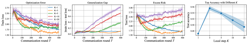
(a) Batch size $b=16$

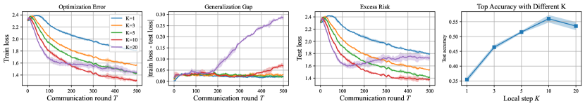
(b) Batch size $b=64$

Figure 4: Proof-of-concept on CIFAR10 experiments with different local batch size $b$.

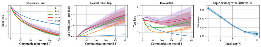
(a) Batch size $b=16$

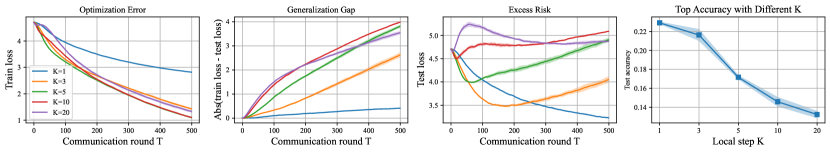
(b) Batch size $b=32$

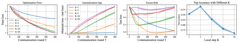
(c) Batch size $b=64$

Figure 5: Proof-of-concept on CIFAR100 experiments with different local batch size $b$.

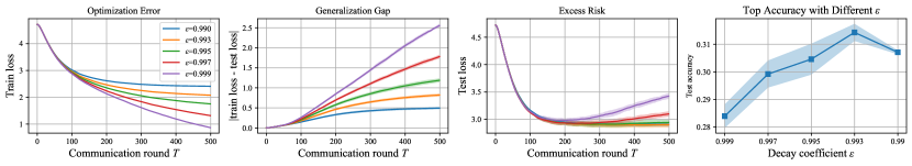
(a) Batch size $b=16$, local steps $K=3$, and learning rate decay $\epsilon$

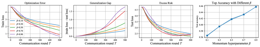
(b) Batch size $b=16$, local steps $K=1$, and server momentum $\beta$

Figure 6: Proof-of-concept on CIFAR100 experiments with global learning rate decay and momentum.

Algorithm 2 FOSM

0:  $\boldsymbol{x}^{0},\eta_{l},\eta_{g},T$

0:  $\boldsymbol{x}^{T}$

1:  for round $t$ $\in$ $[T]$ do

2:     Server broadcast model $\boldsymbol{x}^{t}$

3:     for client $i$ $\in$ $[N]$ in parallel do

4:        $\boldsymbol{x}^{t,0}_{i}=\boldsymbol{x}^{t}$

5:        for local update step $k=0,\dots,K-1$  do

6:           $\boldsymbol{x}^{t,k+1}_{i}=\boldsymbol{x}^{t,k}_{i}-\eta_{l}\boldsymbol{g}_{i}^{t,k}$

7:        end for

8:        Client uploads local updates $\boldsymbol{d}_{i}^{t}=\boldsymbol{x}^{t,0}-\boldsymbol{x}^{t,K}$

9:     end for

10:     Server compute an estimate $\boldsymbol{d}^{t}=\frac{1}{N}\sum_{i\in[N]}\boldsymbol{d}_{i}^{t}$

11:     Server compute momentum $\boldsymbol{m}^{t}=\beta\boldsymbol{m}^{t-1}+\nu\boldsymbol{d}^{t}$

12:     Server updates $\boldsymbol{x}^{t+1}=\boldsymbol{x}^{t}-\eta_{g}\boldsymbol{m}^{t}$

13:  end for

References

• Antunes et al. (2022) Antunes, R. S.; André da Costa, C.; Küderle, A.; Yari, I. A.; and Eskofier, B. 2022. Federated learning for healthcare: Systematic review and architecture proposal. ACM Transactions on Intelligent Systems and Technology (TIST), 13(4): 1–23.
• Barnes, Dytso, and Poor (2022) Barnes, L. P.; Dytso, A.; and Poor, H. V. 2022. Improved information theoretic generalization bounds for distributed and federated learning. In 2022 IEEE International Symposium on Information Theory (ISIT), 1465–1470. IEEE.
• Caldarola, Caputo, and Ciccone (2022) Caldarola, D.; Caputo, B.; and Ciccone, M. 2022. Improving generalization in federated learning by seeking flat minima. In European Conference on Computer Vision, 654–672. Springer.
• Charles and Papailiopoulos (2018) Charles, Z.; and Papailiopoulos, D. 2018. Stability and generalization of learning algorithms that converge to global optima. In International conference on machine learning, 745–754. PMLR.
• Chen, Jin, and Yu (2018) Chen, Y.; Jin, C.; and Yu, B. 2018. Stability and convergence trade-off of iterative optimization algorithms. arXiv preprint arXiv:1804.01619.
• Dwork and Feldman (2018) Dwork, C.; and Feldman, V. 2018. Privacy-preserving prediction. In Conference On Learning Theory, 1693–1702. PMLR.
• Dziugaite and Roy (2017) Dziugaite, G. K.; and Roy, D. M. 2017. Computing nonvacuous generalization bounds for deep (stochastic) neural networks with many more parameters than training data. arXiv preprint arXiv:1703.11008.
• Elisseeff et al. (2005) Elisseeff, A.; Evgeniou, T.; Pontil, M.; and Kaelbing, L. P. 2005. Stability of Randomized Learning Algorithms. Journal of Machine Learning Research, 6(1).
• Ge et al. (2019) Ge, R.; Kakade, S. M.; Kidambi, R.; and Netrapalli, P. 2019. The step decay schedule: A near optimal, geometrically decaying learning rate procedure for least squares. Advances in neural information processing systems, 32.
• Gu et al. (2023) Gu, X.; Lyu, K.; Huang, L.; and Arora, S. 2023. Why (and When) does Local SGD Generalize Better than SGD? In ICLR. OpenReview.net.
• Hardt, Recht, and Singer (2016) Hardt, M.; Recht, B.; and Singer, Y. 2016. Train faster, generalize better: Stability of stochastic gradient descent. In International conference on machine learning, 1225–1234. PMLR.
• Hsu, Qi, and Brown (2019) Hsu, T.-M. H.; Qi, H.; and Brown, M. 2019. Measuring the effects of non-identical data distribution for federated visual classification. arXiv preprint arXiv:1909.06335.
• Huang et al. (2023) Huang, W.; Ye, M.; Shi, Z.; Wan, G.; Li, H.; Du, B.; and Yang, Q. 2023. Federated Learning for Generalization, Robustness, Fairness: A Survey and Benchmark. arXiv preprint arXiv:2311.06750.
• Jain, Kar et al. (2017) Jain, P.; Kar, P.; et al. 2017. Non-convex optimization for machine learning. Foundations and Trends® in Machine Learning, 10(3-4): 142–363.
• Jelassi and Li (2022) Jelassi, S.; and Li, Y. 2022. Towards understanding how momentum improves generalization in deep learning. In International Conference on Machine Learning, 9965–10040. PMLR.
• Jin et al. (2021) Jin, C.; Netrapalli, P.; Ge, R.; Kakade, S. M.; and Jordan, M. I. 2021. On nonconvex optimization for machine learning: Gradients, stochasticity, and saddle points. Journal of the ACM (JACM), 68(2): 1–29.
• Kalimeris et al. (2019) Kalimeris, D.; Kaplun, G.; Nakkiran, P.; Edelman, B.; Yang, T.; Barak, B.; and Zhang, H. 2019. Sgd on neural networks learns functions of increasing complexity. Advances in neural information processing systems, 32.
• Karimireddy et al. (2020) Karimireddy, S. P.; Kale, S.; Mohri, M.; Reddi, S.; Stich, S.; and Suresh, A. T. 2020. Scaffold: Stochastic controlled averaging for federated learning. In International Conference on Machine Learning, 5132–5143. PMLR.
• Kingma and Ba (2014) Kingma, D. P.; and Ba, J. 2014. Adam: A method for stochastic optimization. arXiv preprint arXiv:1412.6980.
• Koloskova et al. (2020) Koloskova, A.; Loizou, N.; Boreiri, S.; Jaggi, M.; and Stich, S. 2020. A unified theory of decentralized sgd with changing topology and local updates. In International Conference on Machine Learning, 5381–5393. PMLR.
• Krizhevsky (2009) Krizhevsky, A. 2009. Learning multiple layers of features from tiny images. Technical report.
• Kuzborskij and Lampert (2018) Kuzborskij, I.; and Lampert, C. 2018. Data-dependent stability of stochastic gradient descent. In International Conference on Machine Learning, 2815–2824. PMLR.
• Lei and Ying (2020) Lei, Y.; and Ying, Y. 2020. Fine-grained analysis of stability and generalization for stochastic gradient descent. In International Conference on Machine Learning, 5809–5819. PMLR.
• Li, Yu, and He (2019) Li, H.; Yu, L.; and He, W. 2019. The impact of GDPR on global technology development.
• Li, Luo, and Qiao (2019) Li, J.; Luo, X.; and Qiao, M. 2019. On generalization error bounds of noisy gradient methods for non-convex learning. arXiv preprint arXiv:1902.00621.
• Li et al. (2020) Li, T.; Sahu, A. K.; Zaheer, M.; Sanjabi, M.; Talwalkar, A.; and Smith, V. 2020. Federated optimization in heterogeneous networks. Proceedings of Machine learning and systems, 2: 429–450.
• Li et al. (2019) Li, X.; Huang, K.; Yang, W.; Wang, S.; and Zhang, Z. 2019. On the convergence of fedavg on non-iid data. arXiv preprint arXiv:1907.02189.
• Long et al. (2020) Long, G.; Tan, Y.; Jiang, J.; and Zhang, C. 2020. Federated learning for open banking. In Federated learning: privacy and incentive, 240–254. Springer.
• McMahan et al. (2017) McMahan, B.; Moore, E.; Ramage, D.; Hampson, S.; and y Arcas, B. A. 2017. Communication-efficient learning of deep networks from decentralized data. In Artificial intelligence and statistics, 1273–1282. PMLR.
• Neu et al. (2021) Neu, G.; Dziugaite, G. K.; Haghifam, M.; and Roy, D. M. 2021. Information-theoretic generalization bounds for stochastic gradient descent. In Conference on Learning Theory, 3526–3545. PMLR.
• Nguyen et al. (2021) Nguyen, D. C.; Ding, M.; Pathirana, P. N.; Seneviratne, A.; Li, J.; and Poor, H. V. 2021. Federated learning for internet of things: A comprehensive survey. IEEE Communications Surveys & Tutorials, 23(3): 1622–1658.
• Pensia, Jog, and Loh (2018) Pensia, A.; Jog, V.; and Loh, P.-L. 2018. Generalization error bounds for noisy, iterative algorithms. In 2018 IEEE International Symposium on Information Theory (ISIT), 546–550. IEEE.
• Qu et al. (2022) Qu, Z.; Li, X.; Duan, R.; Liu, Y.; Tang, B.; and Lu, Z. 2022. Generalized federated learning via sharpness aware minimization. In International conference on machine learning, 18250–18280. PMLR.
• Reddi et al. (2020) Reddi, S.; Charles, Z.; Zaheer, M.; Garrett, Z.; Rush, K.; Konečnỳ, J.; Kumar, S.; and McMahan, H. B. 2020. Adaptive federated optimization. arXiv preprint arXiv:2003.00295.
• Reisizadeh et al. (2020) Reisizadeh, A.; Farnia, F.; Pedarsani, R.; and Jadbabaie, A. 2020. Robust federated learning: The case of affine distribution shifts. Advances in Neural Information Processing Systems, 33: 21554–21565.
• Shalev-Shwartz et al. (2010) Shalev-Shwartz, S.; Shamir, O.; Srebro, N.; and Sridharan, K. 2010. Learnability, stability and uniform convergence. The Journal of Machine Learning Research, 11: 2635–2670.
• Shi et al. (2023) Shi, Y.; Liu, Y.; Wei, K.; Shen, L.; Wang, X.; and Tao, D. 2023. Make landscape flatter in differentially private federated learning. In Proceedings of the IEEE/CVF Conference on Computer Vision and Pattern Recognition, 24552–24562.
• Sun et al. (2024) Sun, J.; Wu, X.; Huang, H.; and Zhang, A. 2024. On the role of server momentum in federated learning. In Proceedings of the AAAI Conference on Artificial Intelligence, volume 38, 15164–15172.
• Sun et al. (2023) Sun, Y.; Shen, L.; Chen, S.; Ding, L.; and Tao, D. 2023. Dynamic regularized sharpness aware minimization in federated learning: Approaching global consistency and smooth landscape. In International Conference on Machine Learning, 32991–33013. PMLR.
• Sun, Shen, and Tao (2024) Sun, Y.; Shen, L.; and Tao, D. 2024. Understanding how consistency works in federated learning via stage-wise relaxed initialization. Advances in Neural Information Processing Systems, 36.
• Sun, Niu, and Wei (2024) Sun, Z.; Niu, X.; and Wei, E. 2024. Understanding generalization of federated learning via stability: Heterogeneity matters. In International Conference on Artificial Intelligence and Statistics, 676–684. PMLR.
• Teng, Ma, and Yuan (2021) Teng, J.; Ma, J.; and Yuan, Y. 2021. Towards understanding generalization via decomposing excess risk dynamics. arXiv preprint arXiv:2106.06153.
• Voigt and Von dem Bussche (2017) Voigt, P.; and Von dem Bussche, A. 2017. The eu general data protection regulation (gdpr). A Practical Guide, 1st Ed., Cham: Springer International Publishing, 10(3152676): 10–5555.
• Wang et al. (2022) Wang, J.; Das, R.; Joshi, G.; Kale, S.; Xu, Z.; and Zhang, T. 2022. On the unreasonable effectiveness of federated averaging with heterogeneous data. arXiv preprint arXiv:2206.04723.
• Wang et al. (2020) Wang, J.; Liu, Q.; Liang, H.; Joshi, G.; and Poor, H. V. 2020. Tackling the objective inconsistency problem in heterogeneous federated optimization. Advances in neural information processing systems, 33: 7611–7623.
• Wang, Lin, and Chen (2022) Wang, Y.; Lin, L.; and Chen, J. 2022. Communication-efficient adaptive federated learning. In International Conference on Machine Learning, 22802–22838. PMLR.
• Wu and He (2018) Wu, Y.; and He, K. 2018. Group normalization. In Proceedings of the European conference on computer vision (ECCV), 3–19.
• Wu et al. (2023a) Wu, Z.; Xu, Z.; Yu, H.; and Liu, J. 2023a. Information-Theoretic Generalization Analysis for Topology-aware Heterogeneous Federated Edge Learning over Noisy Channels. IEEE Signal Processing Letters.
• Wu et al. (2023b) Wu, Z.; Xu, Z.; Zeng, D.; and Wang, Q. 2023b. Federated generalization via information-theoretic distribution diversification. arXiv preprint arXiv:2310.07171.
• Xu et al. (2021) Xu, J.; Wang, S.; Wang, L.; and Yao, A. C.-C. 2021. Fedcm: Federated learning with client-level momentum. arXiv preprint arXiv:2106.10874.
• Yin, Kannan, and Bartlett (2019) Yin, D.; Kannan, R.; and Bartlett, P. 2019. Rademacher complexity for adversarially robust generalization. In International conference on machine learning, 7085–7094. PMLR.
• You et al. (2019) You, K.; Long, M.; Wang, J.; and Jordan, M. I. 2019. How does learning rate decay help modern neural networks? arXiv preprint arXiv:1908.01878.
• Zeng et al. (2023a) Zeng, D.; Liang, S.; Hu, X.; Wang, H.; and Xu, Z. 2023a. FedLab: A Flexible Federated Learning Framework. Journal of Machine Learning Research, 24(100): 1–7.
• Zeng et al. (2023b) Zeng, D.; Xu, Z.; Pan, Y.; Wang, Q.; and Tang, X. 2023b. Tackling hybrid heterogeneity on federated optimization via gradient diversity maximization. arXiv preprint arXiv:2310.02702.
• Zhang et al. (2021) Zhang, C.; Bengio, S.; Hardt, M.; Recht, B.; and Vinyals, O. 2021. Understanding deep learning (still) requires rethinking generalization. Communications of the ACM, 64(3): 107–115.
• Zhang et al. (2023) Zhang, Y.; Zeng, D.; Luo, J.; Xu, Z.; and King, I. 2023. A Survey of Trustworthy Federated Learning with Perspectives on Security, Robustness, and Privacy. arXiv preprint arXiv:2302.10637.
• Zhou et al. (2020) Zhou, P.; Feng, J.; Ma, C.; Xiong, C.; Hoi, S. C. H.; et al. 2020. Towards theoretically understanding why sgd generalizes better than adam in deep learning. Advances in Neural Information Processing Systems, 33: 21285–21296.
• Zhou, Liang, and Zhang (2018) Zhou, Y.; Liang, Y.; and Zhang, H. 2018. Generalization error bounds with probabilistic guarantee for SGD in nonconvex optimization. arXiv preprint arXiv:1802.06903.