Krylov Complexity in the Schrödinger Field Theory

Abstract

We investigate the Krylov complexity in the context of Schrödinger field theory in the grand canonic ensemble for the bosonic and fermionic cases. Specifically, we find that the Lanczos coefficients $\{a_{n}\}$ and $\{b_{n}\}$ satisfy the linear relations with respect to $n$. It is found that $\{b_{n}\}$ is independent of the chemical potentials while $\{a_{n}\}$ depends on the chemical potentials. The resulting Krylov complexities for both bosonic and fermionic cases behave similarly, which is due to the similar profiles of the square of the absolute values of the auto-correlation functions. In the late time, the Krylov complexity exhibits exponential growth with the asymptotic scaling significantly smaller than the twice of the slope of $\{b_{n}\}$, which is different from that in the relativistic field theory. We argue that this is because the Lanczos coefficients $\{a_{n}\}$ also contributes to the Krylov complexity.

1 Introduction

The complexity of quantum systems refers to the increasing intricacy of their states and operations over time. Studies on quantum complexity in Krylov space have gained much interest in recent years. This type of complexity is known as Krylov complexity. The relevant spectrum of the research spans in many fields, such as: quantum many-body physics Parker:2018yvk ; Rabinovici:2022beu ; Liu:2022god ; Trigueros:2021rwj ; Bhattacharjee:2022ave ; Caputa:2022yju ; Bhattacharjee:2023uwx ; Craps:2024suj , quantum field theory Camargo:2022rnt ; He:2024xjp ; Chattopadhyay:2024pdj ; Malvimat:2024vhr ; Vasli:2023syq ; Kundu:2023hbk ; Avdoshkin:2022xuw ; Khetrapal:2022dzy ; Adhikari:2022whf ; Dymarsky:2021bjq , holographic theories Rabinovici:2023yex , random matrix theory Kar:2021nbm , cosmology Adhikari:2022oxr ; Li:2024ljz ; Li:2024iji ; Li:2024kfm and etc. For a nice review, please refer to Nandy:2024htc and references therein. Since the pioneering work in Parker:2018yvk , the Krylov complexity has become a crucial approach to revealing the information-theoretic facets of quantum dynamics.

In the beginning, Krylov complexity was designed to investigate the integrable and chaotic behaviors of quantum systems as they approach the thermodynamic limit. Investigations indicate that there may be potential correlations between Krylov complexity and physical quantities such as the out-of-time-order correlator (OTOC) Hashimoto:2017oit , eigenstate thermalization hypothesis (ETH) PhysRevE.50.888 , entanglement entropy PhysRevE.99.032213 and Nielsen complexity PhysRevD.100.046020 . People find that Krylov complexity is a well-defined quantity which possesses a clear physical interpretation Parker:2018yvk ; He:2024xjp ; Lv:2023jbv , with the advantage of being easier to be computed compared to other complexities. Specifically, Krylov complexity describes how a wave function spreads through a Hilbert space, corresponding to the growth of operators in the Heisenberg picture, within a special basis known as the Krylov basis. In simpler terms, the (average) position of this wave function is the Krylov complexity, which we will elaborate on in Section 2.1. Moreover, Krylov complexity is also used in the Schrödinger picture, known as spread complexity Balasubramanian:2022tpr , to describe the propagation of quantum states. Krylov complexity has become an active field of research with new discoveries emerging continuously. For more information, see Ganguli:2024uiq ; Fu:2024fdm ; Nandy:2024mml ; Fan:2024iop ; Xu:2024gfm ; Caputa:2024sux ; Baggioli:2024wbz ; Rabinovici:2020ryf ; Bhattacharjee:2022vlt ; Rabinovici:2021qqt ; Caputa:2022eye ; Bhattacharya:2023zqt ; Erdmenger:2023wjg ; Bhattacharjee:2022qjw ; Bhattacharya:2022gbz ; Bhattacharjee:2022lzy ; Camargo:2023eev ; Huh:2023jxt ; Camargo:2024deu ; He:2022ryk ; Caputa:2024vrn ; Hornedal:2022pkc ; Bento:2023bjn ; Nandy:2023brt .

In Ref.Parker:2018yvk , a hypothesis is proposed that in chaotic quantum systems, the Lanczos coefficients $\{b_{n}\}$ should grow as rapidly as possible. The results indicate that the maximum possible growth rate of Lanczos coefficients is linear (with logarithmic corrections in one dimension). Generally, OTOC grows exponentially with large time as $e^{\lambda_{L}t}$ ($\lambda_{L}$ is the Lyapunov exponent), indicating the rapid information scrambling and the sensitivity to the initial conditions. In contrast, Krylov complexity also increases exponentially with large time as $e^{\lambda_{K}t}$, where $\lambda_{K}$ is dubbed the Krylov exponent Parker:2018yvk . It was conjectured that twice of the linear growth rate of the Lanczos coefficients (equivalent to the Krylov exponent) could be an upper limit of the quantum Lyapunov exponent $\lambda_{L}$, i.e., $\lambda_{L}\leq\lambda_{K}$. Although the operator growth hypothesis is effective in distinguishing chaotic and non-chaotic systems in lattice models, it was later found to be ineffective for quantum systems with infinite degrees of freedom, such as quantum field theories (QFTs). It turns out that even in integrable quantum field theories like the free scalar field, the Krylov complexity still exhibits exponential growth Dymarsky:2019elm ; Dymarsky:2021bjq . This suggests that there may still be many subtle aspects of Krylov complexity in quantum field theory.

In this paper, we will study the Krylov complexity in the Schrödinger field theory altland2010condensed . The development of Schrödinger field theory began in 1926 when Austrian physicist Erwin Schrödinger proposed the Schrödinger equation, which became the foundation of quantum mechanics. Schrödinger field theory, as a non-relativistic field theory, was subsequently used to describe quantum fields that follow the Schrödinger equation, especially in the context of many-body systems and situations where the number of particles changes. Over time, Schrödinger field theory has been widely applied in Bose-Einstein condensates, the Bogolyubov–de Gennes equations for superconductors, superfluids, and many-body theory, and has become an indispensable part of modern physics harris2014pedestrian ; Mintchev:2022xqh . The Schrödinger field operator is not a Hermitian operator, hence it is more troublesome to handle compared to the Krylov complexity of the free scalar field Camargo:2022rnt ; He:2024xjp . This is because there is no relationship $O^{\dagger}=O$, at this time the Lanczos coefficients have two sequences $\{a_{n}\}$ and $\{b_{n}\}$, and when dealing with two-point functions, the simplification of calculations using the Hermitian operator cannot be utilized. In this paper, we study the Krylov complexity in bosonic and fermionic case with the grand canonical ensemble, as the chemical potential is less than or equal to zero. We find that the Lanczos coefficients $\{a_{n}\}$ and $\{b_{n}\}$ are both linear with respect to $n$. It is interesting to see that $\{b_{n}\}$ is independent of the chemical potentials while $\{a_{n}\}$ depends on it. Regardless of the bosonic or the fermionic case, the behavior of Krylov complexities are always similar, which is due to the similar behaviors of the square of the absolute values for the auto-correlation function $\lvert\varphi_{0}(t)\rvert^{2}$. In the late time, the Krylov complexity approaches exponential growth. Interestingly, we find that the asymptotic exponential scaling of the Krylov complexity is always smaller than the twice of the slope of $\{b_{n}\}$, which is different from the relativistic free scalar field where the asymptotic exponential scaling of the Krylov complexity is roughly twice of the slope of $\{b_{n}\}$. We attribute this discrepancy to the existence of another Lanczos coefficients $\{a_{n}\}$ in the non-relativistic Schrödinger field theory.

This paper is organized as the following. In Section 2, we will introduce the theoretical foundations of the Krylov complexity, including the construction of the Krylov basis, the computation of Lanczos coefficients, and the interrelation between the Wightman function and the spectral function. In Section 3, we will provide a basic introduction to the Schrödinger field theory, and discuss how to derive the spectral function from the theory as well as present the Wightman power spectral. In Section 4, we will calculate the Lanczos coefficients for both bosonic and fermionic cases in the Schrödinger field theory, and analyze the behavior of Krylov complexity under various chemical potentials. Section 5 will provide a summary of this paper.

2 Preliminaries

In order to facilitate the reader’s understanding and ensure the paper is self-contained, we will provide a detailed introduction to the basics of Krylov complexity in this section.

2.1 Krylov complexity

In the quantum theory, a Heisenberg operator $O(t)$ satisfies the Heisenberg equation sakurai2020modern

$$\partial_{t}O(t)=i[H,O(t)],$$ (1)

where $H$ is the time-independent Hamiltonian. The operator $O(t)$ can be Hermitian or non-Hermitian. One can introduce a superoperator $\mathcal{L}\equiv[H,\cdot]$ such that

$$\mathcal{L}O(t)\equiv[H,O(t)].$$ (2)

Then we have

$$\partial_{t}O(t)=i\mathcal{L}O(t).$$ (3)

This form looks like the Schrödinger equation for a state, which has a formal solution

$$O(t)=e^{i\mathcal{L}t}\mathcal{O}(0)=\sum_{n=0}^{\infty}\frac{(it)^{n}}{n!}\mathcal{L}^{n}O,$$ (4)

where $O\equiv O(0)$ and

$$\mathcal{L}^{0}O=O,\qquad\mathcal{L}O=[H,O],\qquad\mathcal{L}^{2}O=[H,[H,O]],\qquad\cdots.$$ (5)

The operator $O(t)$ belongs to a subspace of operators, known as the Krylov space, which is spanned by $\{\mathcal{L}^{n}O\},n=0,1,2,\cdots$. The Krylov space is also a Hilbert space, and one can define an inner product for it. One can define the Hilbert space vector as $\left|A\right)$ corresponding to operator $A$, then the inner product can be formulated as Parker:2018yvk ; Caputa:2021sib

$$(A|B)^{g}_{\beta}=\int_{0}^{\beta}g(\lambda)\expectationvalue{e^{\lambda H}A^{\dagger}e^{-\lambda H}B}_{\beta}d\lambda.$$ (6)

In this formula, $\beta$ is the inverse temperature, while $\expectationvalue{\cdots}_{\beta}$ is the thermal expectation value

$$\expectationvalue{A}_{\beta}=\frac{1}{Z}\tr(e^{-\beta H}A),\quad Z=\tr(e^{-\beta H}).$$ (7)

In order for (6) to be a suitable inner product, the function $g(\lambda)$ should satisfy

$$g(\lambda)\geq 0,\qquad g(\beta-\lambda)=g(\lambda),\qquad\frac{1}{\beta}\int_{0}^{\beta}d\lambda g(\lambda)=1.$$ (8)

One can notice that

$$\expectationvalue{e^{\lambda H}A^{\dagger}e^{-\lambda H}\mathcal{L}B}_{\beta}=\expectationvalue{e^{-\lambda H}(\mathcal{L}A)^{\dagger}e^{-\lambda H}B}_{\beta},$$ (9)

which indicates that $\mathcal{L}$ is a Hermitian operator in Krylov space. Assuming that $O$ is normalized initially, then

$$\expectationvalue{e^{\lambda H}O^{\dagger}(t)e^{-\lambda H}O(t)}_{\beta}=\expectationvalue{e^{\lambda H}O^{\dagger}(0)e^{-\lambda H}O(0)}_{\beta}.$$ (10)

This implies that regardless of whether the operator $O$ is Hermitian or not, an operator that is normalized initially will always remain normalized as it evolves over time.

In the Krylov space, $\{\mathcal{L}^{n}O\}$ is the basis as we mentioned above, but such a basis is typically neither orthogonal nor normalized. We aim to construct an orthonormal basis, known as the Krylov basis $\{\left|O_{n}\right)\}$, which can be constructed from the Gram-Schmidt orthogonalization process. The Gram-Schmidt orthogonalization process is a method that involves the following procedures geroch2013quantum . Let $\xi,\eta_{1},\eta_{2},\cdots,\eta_{n}$ be elements of the Hilbert space $\mathcal{H}$. Then

$$\xi=u_{1}\eta_{1}+\cdots+u_{n}\eta_{n}+\tau,\qquad(u_{i}\in\mathbb{C},{\rm and}~{}(\eta_{i},\tau)=0),$$ (11)

where $(\eta,\tau)$ denotes the inner product of $\eta$ and $\tau$ in the Hilbert space, and $\tau$ is also a vector in Hilbert space. That is to say, any vector in $\mathcal{H}$ can be written as a linear combination of $\eta_{1},\cdots,\eta_{n}$, plus a vector $\tau$ perpendicular to the $\eta$’s. It is evident that in the Krylov space, there is

$$\mathcal{L}\left|O_{n}\right)=\sum_{m=0}^{n}{\alpha^{n}}_{m}\left|O_{m}\right)+b_{n+1}\left|O_{n+1}\right),$$ (12)

where ${\alpha^{n}}_{m}=\left(O_{m}\right|\mathcal{L}\left|O_{n}\right)$, $b_{n+1}=\left(O_{n+1}\right|\mathcal{L}\left|O_{n}\right)$. If $\{{\alpha^{n}}_{m}\}$ and $\{b_{n}\}$ are real numbers, then

$$b_{n+1}={\alpha^{n}}_{n+1}={\alpha^{n+1}}_{n}.$$ (13)

It can also be seen that

$$\left(O_{m}\right|\mathcal{L}\left|O_{n}\right)=\left(O_{n}\right|\mathcal{L}\left|O_{m}\right)={\alpha^{n}}_{m}={\alpha^{m}}_{n}=0,\qquad\text{for}\ m-n\geq 2~{}\text{and}~{}n\geq 0.$$ (14)

Specifically, Let $\left|O_{0}\right)=\left|O\right)$ be a normalization operator, then

$$\mathcal{L}\left|O_{0}\right)=a_{0}\left|O_{0}\right)+b_{1}\left|O_{1}\right).$$ (15)

Following the notation of (12), here we have defined $a_{0}={\alpha^{0}}_{0}=\left(O_{0}\right|\mathcal{L}\left|O_{0}\right)$. Subsequently, we can set

$$a_{n}={\alpha^{n}}_{n}=\left(O_{n}\right|\mathcal{L}\left|O_{n}\right).$$ (16)

Following the previous operations, we have

$$\mathcal{L}\left|O_{1}\right) = b_{1}\left|O_{0}\right)+a_{1}\left|O_{1}\right)+b_{2}\left|O_{2}\right),$$ (17)

$$\mathcal{L}\left|O_{2}\right) = b_{2}\left|O_{1}\right)+a_{2}\left|O_{2}\right)+b_{3}\left|O_{3}\right),$$

$$\cdots$$

$$\mathcal{L}\left|O_{n}\right) = b_{n}\left|O_{n-1}\right)+a_{n}\left|O_{n}\right)+b_{n+1}\left|O_{n+1}\right),$$

$$\cdots$$

These two sequences $\{b_{n}\}$ and $\{a_{n}\}$ are called the Lanczos coefficients. In the Krylov space, the operator can be expressed as Parker:2018yvk

$$\left|O(t)\right)=\sum_{n=0}^{\infty}i^{n}\varphi_{n}(t)\left|O_{n}\right),$$ (20)

where $\varphi_{n}(t)=(O_{n}|O(t))$. It is not difficult to see that $\varphi_{n}(0)=\delta_{n0}$ and $\varphi_{n}(t)=0$ for $n<0$. The vector $\left|O(t)\right)$ is always normalized, which is equivalent to

$$\sum_{n}\absolutevalue{\varphi_{n}(t)}^{2}=1.$$ (21)

Substituting (20) into Heisenberg equation (1), the left side of the equation (1) becomes

$$\partial_{t}\left|O(t)\right)=\sum_{n=0}^{\infty}i^{n}\partial_{t}\varphi_{n}(t)\left|O_{n}\right),$$ (22)

and the right side turns into

$$i\mathcal{L}\left|O(t)\right) =\sum_{n=0}^{\infty}i^{n+1}\varphi_{n}(t)\mathcal{L}\left|O_{n}\right)$$ (23)

$$=\sum_{n=0}^{\infty}i^{n+1}\varphi_{n}(t)\left[b_{n}\left|O_{n-1}\right)+a_{n}\left|O_{n}\right)+b_{n+1}\left|O_{n+1}\right)\right]$$

$$=\sum_{n=0}^{\infty}i^{n}[i^{2}\varphi_{n+1}b_{n+1}+ia_{n}\varphi_{n}(t)+b_{n}\varphi_{n-1}(t)]\left|O_{n}\right),$$

where we have taken $b_{0}=0$. Then by matching the coefficients of $\left|O_{n}\right)$, we get the discrete Schrödinger equation

$$\partial_{t}\varphi_{n}(t)=ia_{n}\varphi_{n}(t)+b_{n}\varphi_{n-1}(t)-b_{n+1}\varphi_{n+1}(t).$$ (24)

Now, we can see that the evolution of operators over time, or the growth of operators, has now become a hopping problem on a one-dimensional chain. In this paper, the Krylov complexity is defined as Dymarsky:2021bjq

$$K(t)=1+\sum_{n=0}^{\infty}n\absolutevalue{\varphi_{n}(t)}^{2},$$ (25)

in order to be consistent with previous literatures in quantum field theory He:2024xjp . We need to stress that the growth of operators directly corresponds to an increase in the number of contributing $n$, but this does not necessarily mean that the Krylov complexity will monotonically increase with the growth of the operators. The detailed discussions can be found in He:2024xjp .

To obtain the Krylov complexity, one must first derive the Lanczos coefficients and solve the discrete Schrödinger equation (24). The Lanczos coefficients can be obtained through the so-called moment method viswanath1994recursion , where the moments are defined as

$$\mu_{n}\equiv\left(O\right|\mathcal{L}^{n}\left|O\right)=\left(O\right|\left.(-i)^{n}\frac{d^{n}}{dt^{n}}\left|O(t)\right)\right|_{t=0}=(-i)^{n}\left.\frac{d^{n}}{dt^{n}}\varphi_{0}(t)\right|_{t=0}.$$ (26)

In the second equality, we have employed the Heisenberg equation. In order to compute the moments, one can introduce an extremely important quantity known as the auto-correlation function

$$C(t): =(O(t)|O)=\varphi_{0}^{\ast}(t),$$ (27)

and the Wightman two-point function,

$$\Pi^{W}(t) =\varphi_{0}(t)=(O|O(t))=\expectationvalue{e^{\beta H/2}O^{\dagger}(0)e^{-\beta H/2}O(t)}_{\beta}$$ (28)

$$=\expectationvalue{O^{\dagger}(0)e^{iH(t+i\beta/2)}O(0)e^{-iH(t+i\beta/2)}}_{\beta}$$

$$=\expectationvalue{O^{\dagger}(0)O(t+i\beta/2)}_{\beta}.$$

Here, we have taken the inner product to be the Wightman inner product

$$(A|B)=\expectationvalue{e^{H\beta/2}A^{\dagger}e^{-H\beta/2}B}_{\beta},$$ (29)

which means taking $g(\lambda)=\delta(\lambda-\beta/2)$ in Eq.(6). The autocorrelation function (27) can also be written as:

$$C(t)=\expectationvalue{O^{\dagger}(t-i\beta/2)O(0)}_{\beta}.$$ (30)

The Fourier transform of the auto-correlation function is referred to as the Wightman power spectrum

$$f^{W}(\omega)=\int_{-\infty}^{\infty}dte^{i\omega t}C(t).$$ (31)

The moments (26) then can be rewritten in terms of $f^{W}(\omega)$ as,

$$\mu_{n}=\frac{1}{2\pi}\int_{-\infty}^{\infty}d\omega\omega^{n}[f^{W}(\omega)]^{\ast}.$$ (32)

Since $\mu_{0}=1$, $f^{W}(\omega)$ should satisfy the normalization condition

$$1=\frac{1}{2\pi}\int_{-\infty}^{\infty}d\omega[f^{W}(\omega)]^{\ast}.$$ (33)

Once we have obtained the moments, we can calculate the Lanczos coefficients through the following recurrence relations viswanath1994recursion

$$M^{(n)}_{k} = L^{(n-1)}_{k}-L^{(n-1)}_{n-1}\frac{M^{(n-1)}_{k}}{M^{(n-1)}_{n-1}},$$ (34)

$$L^{(n)}_{k} = \frac{M^{(n)}_{k+1}}{M^{(n)}_{n}}-\frac{M^{(n-1)}_{k}}{M^{(n-1)}_{n-1}},$$ (35)

where $n=1,\cdots,2K$, $k=n,\cdots,2K-n+1$ and

$$M^{(0)}_{k}=(-1)^{k}\mu_{k},\qquad L^{(0)}_{k}=(-1)^{k+1}\mu_{k+1},\qquad k=0,\cdots,2K.$$ (36)

The resulting Lanczos coefficients are

$$b_{n}^{2}=M^{(n)}_{n},\qquad a_{n}=-L^{(n)}_{n},\qquad n=0,\cdots,K.$$ (37)

These equations may seem complicated, but they are not difficult to operate in practice. We just need to regard $M^{(n)}_{k}$ and $L^{(n)}_{k}$ as two matrices, $k$ as the row index, and $n$ as the column index. Then, once we have calculated the $n$-th column of $M$, we can calculate the $n$-th column of $L$. After obtaining these coefficients, we can use the Runge-Kutta method in the time direction to solve the discrete Schrödinger equation to obtain $\varphi_{n}(t)$ (see Appendix A). Consequently, we can compute $K(t)$ based on the definition of Krylov complexity.

2.2 Wightman function and spectral function

In quantum field theory, various correlation functions can be represented by spectral functions. We will demonstrate that the auto-correlation function $C(t)$ or Wightman power spectrum $f^{W}(\omega)$ can also be derived from the spectral functions. Similar operations can also be referred to in Camargo:2022rnt .

Consider two bosonic (fermionic) operators $\phi_{a}$ and $\psi_{b}$, with subscripts used to denote some internal degrees of freedom. We hereby declare that for the bosonic operator $\psi_{b}\equiv\phi_{b}^{\dagger}$, and for the fermionic operator $\psi_{b}\equiv\bar{\phi}_{b}=\phi^{\dagger}_{b}\gamma^{0}$, where $\gamma^{0}$ is the Dirac matrix peskin2018introduction ; kapusta2007finite . Define the Wightman function as

$$D^{>}_{ab}(t,\mathbf{x};t^{\prime},\mathbf{x}^{\prime})\equiv\expectationvalue{\phi_{a}(t,\mathbf{x})\psi_{b}(t^{\prime},\mathbf{x}^{\prime})}_{\beta},$$ (38)

$$D^{<}_{ab}(t,\mathbf{x};t^{\prime},\mathbf{x}^{\prime})\equiv\eta\expectationvalue{\psi_{b}(t^{\prime},\mathbf{x^{\prime}})\phi_{a}(t,\mathbf{x})}_{\beta}.$$ (39)

For the bosonic field $\eta=1$, while for the fermionic field $\eta=-1$. Use $O(t)=e^{iHt}Oe^{-iHt}$, we have

$$\phi_{a}(t+i\beta,\mathbf{x})=e^{-\beta H}\phi_{a}(t,\mathbf{x})e^{\beta H}.$$ (40)

From this equation, one can prove the Kubo-Martin-Schwinger (KMS) relation in the configuration space as

$$D^{<}_{ab}(t+i\beta,\mathbf{x};t^{\prime},\mathbf{x}^{\prime})=\eta D_{ab}^{>}(t,\mathbf{x};t^{\prime},\mathbf{x}^{\prime}).$$ (41)

Assuming that the system has translational symmetries in both time and space directions, we can reach

$$D^{>}_{ab}(t,\mathbf{x};t^{\prime},\mathbf{x}^{\prime})=D^{>}_{ab}(t-t^{\prime},\mathbf{x}-\mathbf{x}^{\prime}),$$ (42)

$$D^{<}_{ab}(t,\mathbf{x};t^{\prime},\mathbf{x}^{\prime})=D^{<}_{ab}(t-t^{\prime},\mathbf{x}-\mathbf{x}^{\prime}).$$ (43)

Without loss of generality, we can let $(t^{\prime}=0,\mathbf{x}^{\prime}=\mathbf{0})$, and perform a Fourier transform on the Wightman function to obtain

$$D^{>}_{ab}(\omega,\mathbf{k})=\int_{-\infty}^{\infty}dt\int d^{d-1}\mathbf{x}e^{i(\omega t-\mathbf{k}\cdot\mathbf{x})}D^{>}_{ab}(t,\mathbf{x};0,\mathbf{0}),$$ (44)

$$D^{<}_{ab}(\omega,\mathbf{k})=\int_{-\infty}^{\infty}dt\int d^{d-1}\mathbf{x}e^{i(\omega t-\mathbf{k}\cdot\mathbf{x})}D^{<}_{ab}(t,\mathbf{x};0,0).$$ (45)

Utilizing the KMS relation in configuration space allows one to derive the KMS relation in the momentum space

$$D^{>}_{ab}(\omega,\mathbf{k})=\eta e^{\beta\omega}D^{<}_{ab}(\omega,\mathbf{k}).$$ (46)

The one can introduce a new correlation function

$$\rho_{ab}(t,\mathbf{x};t^{\prime},\mathbf{x}^{\prime})=\expectationvalue{[\phi_{a}(t,\mathbf{x}),\psi_{b}(t^{\prime},\mathbf{x}^{\prime})]_{\mp}}_{\beta},$$ (47)

in which $[\cdot,\cdot]_{\mp}$ takes the commutator for the bosonic field or the anticommutator for the fermionic field. Its Fourier transform is referred to as the spectral density or spectral function

$$\rho_{ab}(\omega,\mathbf{k})=D^{>}_{ab}(\omega,\mathbf{k})-D^{<}_{ab}(\omega,\mathbf{k}).$$ (48)

From (46) and (48), one can get

$$D^{>}_{ab}(\omega,\mathbf{k})=\frac{\eta e^{\beta\omega}}{\eta e^{\beta\omega}-1}\rho_{ab}(\omega,\mathbf{k}),$$ (49)

$$D^{<}_{ab}(\omega,\mathbf{k})=\frac{1}{\eta e^{\beta\omega}-1}\rho_{ab}(\omega,\mathbf{k}).$$ (50)

In order to calculate the Krylov complexity of the bosonic (fermionic) operator, we can define

$$\Pi^{W}_{ab}(t,\mathbf{x})=\expectationvalue{\psi_{b}(0,\mathbf{0})\phi_{a}(t+i\beta/2,\mathbf{x})}_{\beta}=\eta D_{ab}^{<}(t+i\beta/2,\mathbf{x};0,\mathbf{0}).$$ (51)

Then we have

$$\Pi^{W}(t)=\Pi^{W}_{ab}(t,\mathbf{0}).$$ (52)

Performing a Fourier transform on (51) yields

$$\Pi^{W}_{ab}(\omega,\mathbf{k}) =\eta\int dt\int d^{d-1}\mathbf{x}e^{i(\omega t-\mathbf{k}\cdot\mathbf{x})}D^{<}_{ab}(t+i\beta/2,\mathbf{x};0,\mathbf{0})$$ (53)

$$=\eta\int dt\int d^{d-1}\mathbf{x}e^{\beta\omega/2}e^{i(\omega t-\mathbf{k}\cdot\mathbf{x})}D^{<}_{ab}(t,\mathbf{x};0,\mathbf{0})$$

$$=\eta e^{\beta\omega/2}D^{<}_{ab}(\omega,\mathbf{k})$$

$$=\frac{\eta e^{\frac{\beta\omega}{2}}}{\eta e^{\beta\omega}-1}\rho_{ab}(\omega,\mathbf{k}).$$

Then we can readily get

$$f^{W}(\omega) =\int_{-\infty}^{\infty}dte^{i\omega t}[\Pi^{W}(t)]^{\ast}=\int_{-\infty}^{\infty}dt\int d^{d-1}\mathbf{x}e^{i\omega t}[\Pi^{W}_{ab}(t,\mathbf{x})]^{\ast}\delta^{(d-1)}(\mathbf{x}-\mathbf{0})$$ (54)

$$=\int_{-\infty}^{\infty}dt\int d^{d-1}\mathbf{x}\int\frac{d\omega^{\prime}}{2\pi}\int\frac{d^{d-1}\mathbf{k}}{(2\pi)^{d-1}}e^{i\omega t}[e^{-i(\omega^{\prime}t-\mathbf{k}\cdot\mathbf{x})}\Pi^{W}_{ab}(\omega^{\prime},\mathbf{k})]^{\ast}\delta^{(d-1)}(\mathbf{x}-\mathbf{0})$$

$$=\int d\omega^{\prime}\int\frac{d^{d-1}\mathbf{k}}{(2\pi)^{d-1}}[\Pi^{W}_{ab}(\omega^{\prime},\mathbf{k})]^{\ast}\delta(\omega+\omega^{\prime})=\int\frac{d^{d-1}\mathbf{k}}{(2\pi)^{d-1}}[\Pi^{W}_{ab}(-\omega,\mathbf{k})]^{\ast}$$

$$=\frac{\eta e^{-\frac{\beta\omega}{2}}}{\eta e^{-\beta\omega}-1}\int\frac{d^{d-1}\mathbf{k}}{(2\pi)^{d-1}}[\rho_{ab}(-\omega,\mathbf{k})]^{\ast}.$$

3 Wightman power spectrum of Schrödinger field theory

In the Schrödinger field theory, the Lagrangian for the non-relativistic free bosons and fermions with mass $m$ is given by

$$\mathscr{L}=\psi^{\dagger}\left(i\frac{\partial}{\partial t}+\frac{\nabla^{2}}{2m}\right)\psi.$$ (55)

It is easy to check that the Euler-Lagrange equations derived from this Lagrangian are indeed the Schrödinger equation. If $\psi$ is an operator with canonical commutation relations, it describes a collection of identical non-relativistic bosons, and while $\psi$ is an operator with canonical anti-commutation relations, the field describes identical fermions Mintchev:2022xqh . This Lagrangian is symmetric under the following global $U(1)$ transformation

$$\psi\rightarrow e^{i\alpha}\psi,\qquad\psi^{\dagger}\rightarrow\psi^{\dagger}e^{-i\alpha}.$$ (56)

The corresponding conserved charge is

$$N=\int d^{d-1}\mathbf{x}\mathscr{N}=\int d^{d-1}\mathbf{x}\psi^{\dagger}\psi,$$ (57)

where $\mathscr{N}$ is the charge density. The conjugate field of $\psi$ is

$$\Pi=\frac{\partial\mathscr{L}}{\partial\dot{\psi}}=i\psi^{\dagger}.$$ (58)

Then we can write down the Hamiltonian density as

$$\mathscr{H}=\Pi\dot{\psi}-\mathscr{L}=\psi^{\dagger}\left(-\frac{\nabla^{2}}{2m}\right)\psi.$$ (59)

In the grand canonical ensemble, the partition function is

$$\mathcal{Z}=\tr(e^{-\beta(H-\mu N)}).$$ (60)

in which $H$ is the Hamiltonian with $H=\int d^{d-1}\mathbf{x}\mathscr{H}$ and $\mu$ is the chemical potential. Consequently, the partition function can be rewritten in the path integral form as

$$\mathcal{Z} =\int\mathcal{D}\Pi\mathcal{D}\psi\exp(\int_{0}^{\beta}d\tau\int d^{d-1}\mathbf{x}(\Pi i\partial_{\tau}\psi-\mathscr{H}+\mu\mathscr{N}))$$ (61)

$$=\int\mathcal{D}\psi^{\dagger}\mathcal{D}\psi\exp{\int_{0}^{\beta}d\tau\int d^{d-1}\mathbf{x}(\mathscr{L}+\mu\mathscr{N})},$$

where $\tau=it$. The inverse of the thermal propagator of the Schrödinger field is

$$\mathcal{D}^{-1}(K)\equiv\mathcal{D}^{-1}(\omega_{n},\mathbf{k})=i\omega_{n}+\frac{\mathbf{k}^{2}}{2m}-\mu,$$ (62)

where $K=(k^{0},\mathbf{k})=(-i\omega_{n},\mathbf{k})$. From the thermal propagator, we can obtain the spectral function as

$$\rho(\omega,\mathbf{k})=2\pi\delta(\xi_{\mathbf{k}}-\omega),\qquad\xi_{\mathbf{k}}=\frac{\mathbf{k}^{2}}{2m}-\mu.$$ (63)

It should be noted that we cannot directly substitute this spectral function into the equation (54) to calculate the Wightman power spectrum, because the field $\psi$ here, in the sense of (29), is not necessarily normalized. Therefore, we can redefine

$$\rho(\omega,\mathbf{k})=\mathcal{N}\delta(\xi_{\mathbf{k}}-\omega)$$ (64)

as the spectral function, where $\mathcal{N}$ is a normalization constant that needs to be determined from the equation (33).

To calculate $f^{W}(\omega)$, we first compute the integral

$$I\equiv\int\frac{d^{d-1}\mathbf{k}}{(2\pi)^{d-1}}[\rho(-\omega,\mathbf{k})]^{\ast}=\mathcal{N}\int\frac{d^{d-1}\mathbf{k}}{(2\pi)^{d-1}}\delta(\xi_{\mathbf{k}}+\omega).$$ (65)

Using the identity

$$\int\frac{d^{d}\mathbf{l}}{(2\pi)^{d}}=\int\frac{d\Omega_{d}}{(2\pi)^{d}}\int_{0}^{\infty}dll^{d-1},\qquad\Omega_{d}\equiv\int d\Omega_{d}=\frac{2\pi^{d/2}}{\Gamma(d/2)},$$ (66)

we have

$$I =\mathcal{N}\Omega_{d-1}\int_{0}^{\infty}dk\frac{k^{d-2}}{(2\pi)^{d-1}}\delta\left(\frac{k^{2}}{2m}-\mu+\omega\right)$$ (67)

$$=\mathcal{N}\Omega_{d-1}\int_{0}^{\infty}dk\frac{k^{d-2}}{(2\pi)^{d-1}}\sqrt{\frac{m}{2(\mu-\omega)}}\delta(k-\sqrt{2m(\mu-\omega)})\Theta(\mu-\omega)$$

$$=\mathcal{N}\Omega_{d-1}\frac{m^{\frac{d-1}{2}}[2(\mu-\omega)]^{\frac{d-3}{2}}}{(2\pi)^{d-1}}\Theta(\mu-\omega).$$

in which $\Theta(x)$ is the Heaviside step function with $\Theta(x<0)=0$ and $\Theta(x\geq 0)=1$. Then, absorbing all constants into $\mathcal{N}$, we get

$$f^{W}(\omega)=\mathcal{N}(\mu,\beta,d,\eta)(\mu-\omega)^{\frac{d-3}{2}}\frac{\eta e^{-\frac{\beta\omega}{2}}}{\eta e^{-\beta\omega}-1}\Theta(\mu-\omega).$$ (68)

For simplicity, in this paper we will only consider the case of five dimensions. Thus, for bosonic fields and fermionic fields, the Wightman power spectrum can be written in the specific form as

$$f^{W}(\omega)=\left\{\begin{aligned} &\mathcal{N}(\mu,\beta,5,1)\frac{(\omega-\mu)}{2}\frac{1}{\sinh\frac{\beta\omega}{2}}\Theta(\mu-\omega),\qquad\text{bosonic field}\\ &\mathcal{N}(\mu,\beta,5,-1)\frac{(\mu-\omega)}{2}\frac{1}{\cosh\frac{\beta\omega}{2}}\Theta(\mu-\omega).\qquad\text{fermionic field}\end{aligned}\right.$$ (69)

4 Lanczos coefficients and Krylov complexity of Schrödinger field theory

Due to the fact that the Wightman power spectrum has different expressions for bosonic and fermionic fields in Eq.(69), we will discuss the bosonic case and the fermionic case separately. In this section, our calculations primarily follow the method in our previous paper He:2024xjp , which involves expanding the Wightman power spectrum into a series form and keeping only the terms that play a major role in the results. However, as $\mu>0$, the integration will range from $-\infty$ to $\mu$, which means the integration region passes through the origin, leading the method of He:2024xjp ineffective. Therefore, in this paper we only consider the case with $\mu\leq 0$.

4.1 Bosonic case

4.1.1 $\mu=0$

When the chemical potential vanishes, i.e., $\mu=0$, the Wightman power spectrum of bosonic field $f^{W}(\omega)$ is

$$f^{W}(\omega)=\mathcal{N}(0,\beta,5,1)\frac{\omega}{2\sinh(\frac{\beta\omega}{2})}\Theta(-\omega).$$ (70)

From the normalization condition (33), the normalization coefficient becomes

$$\mathcal{N}(0,\beta,5,1)=\frac{4\beta^{2}}{\pi}.$$ (71)

Subsequently, from the definition of the moment (32), it is obtained that

$$\mu_{n}=\frac{2(-1)^{n}\left(2^{n+2}-1\right)\beta^{-n}\zeta(n+2)\Gamma(n+2)}{\pi^{2}},$$ (72)

where $\zeta(s)=\sum_{n=1}^{\infty}\frac{1}{n^{s}}$ is the Riemann zeta function, and $\Gamma(z)=\int_{0}^{\infty}t^{z-1}e^{-t}dt$ is the Gamma function.

Consequently, from the recurrence relations in the Section 2.1, we can compute the Lanczos coefficients accordingly. We present the numerical results of the Lanczos coefficients $\{a_{n}\}$ and $\{b_{n}\}$ in Figure 1.

Figure 1: (a) Lanczos coefficients $a_{n}$ in the bosonic case as $\mu=0$; (b) Lanczos coefficients $b_{n}$ in the bosonic case as $\mu=0$.

It is found that the sequences $\{a_{n}\}$ and $\{b_{n}\}$ are almost straight lines with respect to $n$. We obtain the following results after fitting the data in Figure 1,

$$\beta a_{n} \approx -4.00n-3.96,$$ (73)

$$\beta b_{n} \approx 2.00n+0.98.$$ (74)

From equations (27) and (31), it is known that

$$\varphi_{0}(t) =\frac{1}{2\pi}\int_{-\infty}^{\infty}f^{W}(\omega)e^{i\omega t}d\omega$$ (75)

$$=\frac{2\psi^{(1)}\left(\frac{it}{\beta}+\frac{1}{2}\right)}{\pi^{2}},$$

in which $f^{W}$ is from Eq.(70) and $\psi^{(1)}(z)=\frac{d\psi(z)}{dz}$ with $\psi(z)$ the digamma function

$$\psi(z)=\frac{d}{dz}\ln\Gamma(z)=\frac{\Gamma^{\prime}(z)}{\Gamma(z)}.$$ (76)

According to the Schrödinger equation (24), the numerical results of $\varphi_{n}(t)$ can be readily obtained from the Lanczos coefficients and $\varphi_{0}(t)$. During the numerical computation, we need to keep the normalization condition (21) of $\varphi_{n}(t)$.

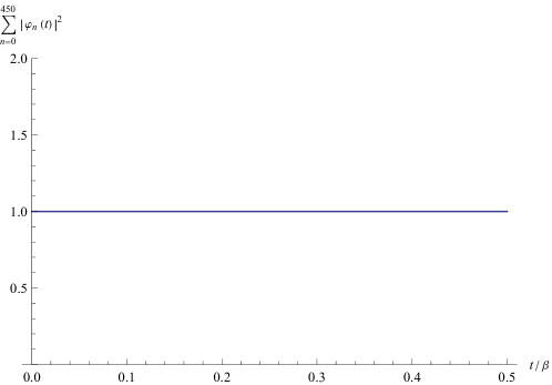
Figure 2: The normalization condition of $\varphi_{n}(t)$ is satisfied during the time evolution.

Figure 2 shows that $\varphi_{n}(t)$ are indeed normalized during the time evolution, which guarantees that our numerical computation of $\varphi_{n}(t)$ is correct. In the calculations, we take the maximum value of $n$ to be $450$, which is sufficiently large within the time range we are considering to get the correct values of $\varphi_{n}(t)$ and the subsequent Krylov complexity. We need to stress that the normalization condition of $\varphi_{n}(t)$ is well satisfied as well in other cases in the following, therefore, we do not intend to show them again. In the Figure 3, we present the numerical results of the Krylov complexity against the time (scaled by $\beta$), in which the vertical axis is in the logarithmic scale. Therefore, as expected, the Krylov complexity exhibits exponential growth behavior in time. The fitted exponential scaling is roughly $\lambda_{K}\approx 2.669/\beta$, which is smaller than the twice the slope of $\{b_{n}\}$ (which is $4/\beta$). This is different from that in the relativistic free scalar field theory He:2024xjp . This discrepancy is due to the fact that another Lanczos coefficient $\{a_{n}\}$ will affect the Krylov complexity. It is noted that the computation of complexity as $a_{n}\neq 0$ is in fact mathematically the same as the usual computation of the spread complexity. In Balasubramanian:2022tpr , the authors found that when the Hamiltonian can be described as generators of a certain Lie algebra, the spread complexity can be calculated using the method of generalized coherent states. They consider an example where the Hamiltonian is a generator of SL(2,R)

$$H=\alpha(L_{-1}+L_{1})+\gamma L_{0}+\delta I,$$ (77)

where $L_{+}$ and $L_{-}$ are raising and lowering ladder operators, and $L_{0}$ belongs to the Cartan subalgebra of the Lie algebra. Then

$$a_{n}=\gamma(h+n)+\delta,\qquad b_{n}=\alpha\sqrt{n(2h+n-1)},$$ (78)

and the complexity is

$$K(t)=\frac{2h}{1-\frac{\gamma^{2}}{4\alpha^{2}}}\sinh^{2}\left(\alpha t\sqrt{1-\frac{\gamma^{2}}{4\alpha^{2}}}\right).$$ (79)

One can verify that when $a_{n}=0$, $K(t)$ will gradually approach a function proportional to $e^{2\alpha t}$ in late time; And when $a_{n}\neq 0$, it will approach a value proportional to $e^{2\alpha\sqrt{1-\frac{\gamma^{2}}{4\alpha^{2}}}t}$, where $\gamma$ (the scaling of $\{a_{n}\}$) contributes to the exponential scaling. From the behavior of $\{a_{n}\}$ and $\{b_{n}\}$, it is impossible to directly discuss the complexity of the Schrödinger field theory using the SL(2,R) Lie algebra. However, we believe that in the Schrödinger field theory, the non-Hermitian nature of the field operators leads to the existence of $a_{n}$, and then this $a_{n}$ will correct the asymptotic behavior of $K(t)$ in a manner similar to the cases in Balasubramanian:2022tpr . This is because the linear relation (by setting $h=1/2$) of $\{a_{n}\}$ and $\{b_{n}\}$ in Eq.(78) are similar to those in our linear case Eqs.(73) and (74), if you are aware of the fact that the Krylov complexity depends much on the behaviors of the Lanczos coefficients.

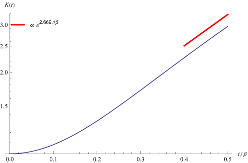
Figure 3: Time evolution of the Krylov complexity $K(t)$ in the bosonic case as $\mu=0$. The vertical axis is in the logarithmic scale. The red line indicates the asymptotic behavior of $K(t)$.

4.1.2 $\mu<0$

As chemical potential $\mu<0$, the Wightman power spectrum $f^{W}(\omega)$ becomes

$$f^{W}(\omega) =\mathcal{N}(\mu,\beta,5,1)\frac{(\omega-\mu)}{2}\frac{1}{\sinh\frac{\beta\omega}{2}}\Theta(\mu-\omega)$$ (80)

$$=\begin{aligned} \mathcal{N}(\mu,\beta,5,1)(\mu-\omega)\sum_{k=0}^{\infty}e^{\beta\omega(k+1/2)},\end{aligned}$$

where we have used the equation

$$\frac{1}{1-x}=\sum_{k=0}^{\infty}x^{k},\qquad\text{for $\absolutevalue{x}<1$.}$$ (81)

From (80) and (33), it is known that

$$\mathcal{N}(\mu,\beta,5,1)=\frac{\pi\beta^{2}e^{-\frac{\beta\mu}{2}}}{2\,_{3}F_{2}\left(\frac{1}{2},\frac{1}{2},1;\frac{3}{2},\frac{3}{2};e^{\beta\mu}\right)},$$ (82)

In which $\,{}_{p}F_{q}$ is the hypergeometric function, defined as

$$\,{}_{p}F_{q}(a_{1},\cdots,a_{p};b_{1},\cdots,b_{q};z)=\sum_{n=0}^{\infty}\frac{(a_{1})_{n}\cdots(a_{p})_{n}}{(b_{1})_{n}\cdots(b_{q})_{n}}\frac{z^{n}}{n!}.$$ (83)

The moments then can be calculated as

$$\mu_{n}= \sum_{k=0}^{\infty}\frac{\beta^{2}(-1)^{n}2^{n-1}e^{-\frac{\beta\mu}{2}}(2\beta k+\beta)^{-n-2}}{\,{}_{3}F_{2}\left(\frac{1}{2},\frac{1}{2},1;\frac{3}{2},\frac{3}{2};e^{\beta\mu}\right)}$$ (84)

$$\times\left[\beta(2k+1)\mu\Gamma\left(n+1,-\frac{1}{2}\beta(2k+1)\mu\right)+2\Gamma\left(n+2,-\frac{1}{2}\beta(2k+1)\mu\right)\right].$$

It should be noted that, whether for the bosonic case or the fermionic case, in our subsequent numerical calculations, the upper limit of this summation is always taken as $k_{\text{max}}=200$.

The numerical results of the Lanczos coefficients $a_{n}$ and $b_{n}$ are presented in the Figure 4 with various chemical potentials. It is interesting to see that the behaviors of $b_{n}$ seem to be unaffected by the chemical potentials, as can be seen in the panel (b) of Figure 4 that they all overlap together for various $\mu$’s.

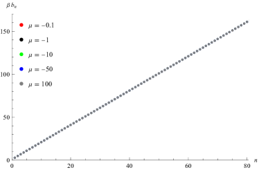
Figure 4: (a) Lanczos coefficients $a_{n}$ in the bosonic case as $\mu<0$ with various chemical potentials; (b) Lanczos coefficients $b_{n}$ in the bosonic case as $\mu<0$ with various chemical potentials. They overlap together.

We fit the linear behavior of the $a_{n}$ and $b_{n}$ against $n$, the data are shown in the Table 1. From the table, we can empirically obtain that the linear fit roughly satisfies

$$\beta a_{n}\approx-4(n+1)-\mu,\qquad\beta b_{n}\approx 2n+1.$$ (85)

Chemical potential	$\beta a_{n}$	$\beta b_{n}$
$0$	$-3.960875810-4.000032607n$	$0.9804415923+2.000016298n$
$-0.1$	$-4.075416651-4.000020537n$	$0.9866122122+2.000011603n$
$-1$	$-4.993572876-4.000005364n$	$0.9955512958+2.000004221n$
$-10$	$-13.99999932-4.000000001n$	$0.9987444215+2.000001570n$
$-50$	$-54.00000000-4.000000000n$	$0.9987447602+2.000001569n$
$-100$	$-104.0000000-4.000000000n$	$0.9987447602+2.000001569n$

Table 1: Data of the linear fit of the Lanczos coefficients $a_{n}$ and $b_{n}$ with respect to $n$, as $\mu\leq 0$ in the bosonic case.

The time evolution of the Krylov complexity is exhibited in the Figure 5, in which the vertical axis is in the logarithmic scale. We can find that it exponentially increases at large time.

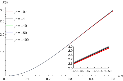
Figure 5: Time evolution of the Krylov complexity in the bosonic case with various chemical potentials. They almost overlap together. The vertical axis is in the logarithmic scale. The inset plot enlarges the figure in the range of $t/\beta\in[0.45,0.5]$.

Besides, it can be seen that as time is short, the Krylov complexities obtained from various chemical potentials almost overlap together; However, as time is longer, they start to differ from each other. And, the larger the chemical potential is, the smaller the Krylov complexity will be. We have listed the asymptotic slope of $K(t)$ in the Table 2. We find that as the chemical potential decreases, the asymptotic slope of $\log K(t)$ increases and approximately approaches $2.746(<4)$ (see the second column for bosonic case).

Chemical potential	Asymptotic slope of $\log K(t)$	Asymptotic slope of $\log K(t)$
$\mu$	(bosonic case in the unit of $1/\beta$)	(fermionic case in the unit of $1/\beta$)
$0$	$2.669$	$2.783$
$-0.1$	$2.682$	$2.780$
$-1$	$2.726$	$2.761$
$-10$	$2.746$	$2.746$
$-50$	$2.746$	$2.746$
$-100$	$2.746$	$2.746$

Table 2: The asymptotic slope of $\log K(t)$ for bosonic and fermionic cases with various chemical potentials.

4.2 Fermionic case

For the fermionic case, the Wightman power spectrum is different from the bosonic case (69), and the operators satisfy the anti-commutative relations. Therefore, we expect that the Krylov complexity in fermionic case will be different from those in bosonic case.

4.2.1 $\mu=0$

For $\mu=0$, the Wightman power spectrum $f^{W}(\omega)$ is

$$f^{W}(\omega)=-\mathcal{N}(0,\beta,5,-1)\frac{\omega}{2}\frac{1}{\cosh(\frac{\beta\omega}{2})}\Theta(\mu-\omega),$$ (86)

where

$$\mathcal{N}(0,\beta,5,-1)=\frac{\pi\beta^{2}}{2G},\qquad G=\sum_{n=0}^{\infty}\frac{(-1)^{n}}{(2n+1)^{2}}.$$ (87)

The corresponding moments are

$$\mu_{n}=\frac{(-1)^{n}2^{-n-4}\beta^{-n}\left(\zeta\left(n+2,\frac{1}{4}\right)-\zeta\left(n+2,\frac{3}{4}\right)\right)\Gamma(n+2)}{G}.$$ (88)

In Figure 6, we present the numerical results for the Lanczos coefficients $a_{n}$ and $b_{n}$. Surprisingly, these results are similar to the bosonic case with a chemical potential of zero in Figure 1.

Figure 6: (a) Lanczos coefficients $a_{n}$ in the fermionic case as $\mu=0$; (b) Lanczos coefficients $b_{n}$ in the fermionic case as $\mu=0$.

The linear fitting of the Lanczos coefficients $a_{n}$ and $b_{n}$ are

$$\beta a_{n} \approx -4.00n-4.01,$$ (89)

$$\beta b_{n} \approx 2.00n+1.00.$$ (90)

Interestingly, we find that these fittings for fermionic case are very close to those in the bosonic case (73) and (74). From (86), we can get the auto-correlation function as

$$\varphi_{0}(t)=\frac{\psi^{(1)}\left(\frac{it}{2\beta}+\frac{1}{4}\right)-\psi^{(1)}\left(\frac{it}{2\beta}+\frac{3}{4}\right)}{16G}.$$ (91)

Based on the Lanczos coefficients and the autocorrelation function (91), we numerically compute the time evolution of the Krylov complexity, please refer to Figure 7. Figure 7(a) shows the Krylov complexity for the fermionic case with $\mu=0$. The vertical axis is in logarithmic scale. Therefore, we can see that at large time, the linear behavior of $K(t)$ indicates the exponential increase of the Krylov complexity at large time. Just as in the bosonic case, the asymptotic behavior of $K(t)$ in the fermionic case is clearly less than twice the slope of $b_{n}$. As shown in the Figure 7(a), the asymptotic behavior of $K(t)$ is proportional to $e^{2.783t/\beta}$. In Figure 7(b), we compare the Krylov complexities of the bosonic and fermionic cases, and it can be seen that at early times the two curves coincide. However, as time grows the two curves will separate, and the fermionic complexity grows a little bit faster than the bosonic one.

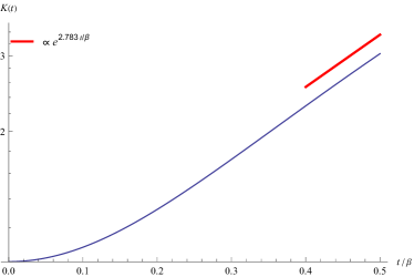
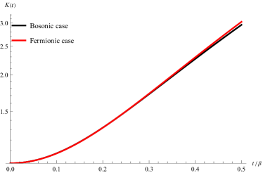
Figure 7: (a) The Krylov complexity for the fermionic case as $\mu=0$. The red line indicates the asymptotic behavior of $K(t)$. (b) The comparison of the Krylov complexity for both bosonic case and fermionic cases as $\mu=0$. At early times, the two complexities overlap, however as time goes by, the two complexities gradually separate.

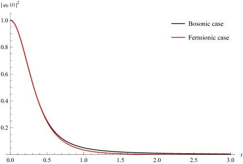
Figure 8: Time evolution of $|\varphi_{0}(t)|^{2}$ for the bosonic and fermionic fields as $\mu=0$.

4.2.2 Digression: the similarities of the Krylov complexity for bosonic and fermionic case

In this subsection we will digress to discuss the similarities of the Krylov complexity between bosonic and fermionic case. From the definition of the Krylov complexity Eq.(25), we see that the Krylov complexity depends on the wave function $\varphi_{n}(t)$. Moreover, from the discrete Schrödinger equation (24), it is found that $\varphi_{n}(t)$ is related to the Lanczos coefficients $a_{n}$ and $b_{n}$ as well as the auto-correlation function $\varphi_{0}(t)$. As we already known, the numerical values of the Lanczos coefficients for the bosonic and fermionic fields are very close to each other for $\mu=0$, see Eqs.(73)-(74) and Eqs.(89)-(90). Therefore, we speculate that the small discrepancies of the Krylov complexity between the bosonic and fermionic fields may come from the small differences between the auto-correlation function $\varphi_{0}(t)$. To this end, we compute and compare the time evolution of $\lvert\varphi_{0}(t)\lvert^{2}$ for both bosonic and fermionic fields in Figure 8. From this figure we can see that at the early times, the two curves for $\lvert\varphi_{0}(t)\lvert^{2}$ overlap together, but at around $t/\beta\sim 0.5$, they start to separate from each other. This behavior is consistent with the corresponding time evolutions of $K(t)$ in Figure 7(b) that at around $t/\beta\sim 0.5$ the Krylov complexity starts to diverse from each other in numerics.

However, despite of the differences, we can also see that the trend of Krylov complexity for both bosonic and fermionic fields are similar. This is due to the similarities of the Lanczos coefficients ($a_{n}$ and $b_{n}$) and the resemblances of the $|\varphi_{0}(t)|^{2}$ (although with some small differences). In the following we will see that $\lvert\varphi_{n}(t)\rvert^{2}$ actually will only depends on the Lanczos coefficient $b_{n}$ and the auto-correlation function $\varphi_{0}(t)$, rather than depending on the Lanczos coefficient $a_{n}$. We can assume

$$x_{n}=\epsilon n,\varphi_{n}(t)=\varphi(x_{n},t),~{}{\rm and}~{}a_{n}=a(x_{n}),b_{n}=b(x_{n}),$$ (92)

in which $\epsilon$ plays the role of the lattice spacing. That is to say, we are going to transform the problem of discrete $n$ to the problem of continuous $x_{n}$ with the small lattice spacing $\epsilon$. Then the discrete Schrödinger equation (24) becomes

$$\partial_{t}\varphi(x_{n},t)=ia(x_{n})\varphi(x_{n},t)+b(x_{n})\varphi(x_{n}-\epsilon,t)-b(x_{n}+\epsilon)\varphi(x_{n}+\epsilon,t).$$ (93)

We can multiply $\varphi^{\ast}(x_{n},t)$ to both sides of the above equation,

$$\varphi^{\ast}(x_{n},t)\partial_{t}\varphi(x_{n},t)=ia(x_{n})\absolutevalue{\varphi(x_{n},t)}^{2}+b(x_{n})\varphi(x_{n}-\epsilon,t)\varphi^{\ast}(x_{n},t)-b(x_{n}+\epsilon)\varphi(x_{n}+\epsilon,t)\varphi^{\ast}(x_{n},t).$$ (94)

Make the complex conjugate of the above equation, and add them together, then the left hand side becomes

$$\text{L.H.S.}=\varphi^{\ast}(x,t)\partial_{t}\varphi(x,t)+\varphi(x,t)\partial_{t}\varphi^{\ast}(x,t)=\partial_{t}\absolutevalue{\varphi(x_{n},t)}^{2}.$$ (95)

The right hand side becomes (expand to the order of $\epsilon$)

$$\text{R.H.S.}= b(x_{n})\left[\varphi(x_{n}-\epsilon,t)\varphi^{\ast}(x_{n},t)+\varphi^{\ast}(x_{n}-\epsilon,t)\varphi(x_{n},t)\right]-$$ (96)

$$b(x_{n}+\epsilon)\left[\varphi(x_{n}+\epsilon,t)\varphi^{\ast}(x_{n},t)+\varphi^{\ast}(x_{n}+\epsilon,t)\varphi(x_{n},t)\right]$$

$$\approx b(x_{n})[2\absolutevalue{\varphi(x_{n},t)}^{2}-\epsilon\partial_{x}\absolutevalue{\varphi(x_{n},t)}^{2}]-b(x_{n}+\epsilon)[2\absolutevalue{\varphi(x_{n},t)}^{2}+\epsilon\partial_{x}\absolutevalue{\varphi(x_{n},t)}^{2}]$$

$$= 2\absolutevalue{\varphi(x_{n},t)}^{2}[b(x_{n})-b(x_{n}+\epsilon)]-\epsilon\partial_{x}\absolutevalue{\varphi(x_{n},t)}^{2}[b(x_{n})+b(x_{n}+\epsilon)]$$

$$\approx -2\epsilon\absolutevalue{\varphi(x_{n},t)}^{2}\partial_{x}b(x_{n})-2\epsilon\partial_{x}\absolutevalue{\varphi(x_{n},t)}^{2}b(x_{n}).$$

Thus, we obtain the following equation (where we have set $x_{n}\equiv x$ and $\Psi(x,t)\equiv\absolutevalue{\varphi(x,t)}^{2}$),

$$\partial_{t}\Psi(x,t)=-2\epsilon\Psi(x,t)\partial_{x}b(x)-2\epsilon\partial_{x}\Psi(x,t)b(x)=-2\epsilon\partial_{x}\left[\Psi(x,t)b(x)\right].$$ (97)

This is a partial differential equation of $|\varphi(x,t)|^{2}$ and $b_{n}$. However, we see that it is nothing to do with the Lanczos coefficient $a_{n}$ in the Eq.(97). Therefore, $a_{n}$ has no influence on the evolution of $|\varphi(x,t)|^{2}$.

We can solve the above equation (97) on an integral curve in the following. Assuming there is a smooth vector field $V=(\frac{dx}{ds},\frac{dt}{ds})$ on the $t-x$ plane, the integral curves of this vector field are parameterized by $s$, satisfying

$$\frac{dt}{ds}=1,\qquad\frac{dx}{ds}=2\epsilon b(x).$$ (98)

Therefore, on this integral curve we have

$$\frac{dx}{dt}=2\epsilon b(x).$$ (99)

Assuming again that this integral curve passes through the point ($x=0,t=\tau$), then this curve is given by

$$\int_{0}^{x}\frac{dx^{\prime}}{2\epsilon b(x^{\prime})}=t-\tau.$$ (100)

in which $\tau$ can be used to label different integral curves. On this single integral curve, we have

$$\frac{d}{dt}\Psi(x,t) =\partial_{t}\Psi(x,t)+\partial_{x}\Psi(x,t)\frac{dx}{dt}$$ (101)

$$=-2\epsilon\Psi(x,t)\partial_{x}b(x).$$

The solution to the above equation is

$$\Psi(x,t)=\Psi(0,\tau)\frac{b(0)}{b(x)}=\Psi\left(0,t-\int_{0}^{x}\frac{dx^{\prime}}{2\epsilon b(x^{\prime})}\right)\frac{b(0)}{b(x)}.$$ (102)

Therefore, as long as we know $\varphi(0,t)$ (equivalent to know $\Psi(0,t)$) and $b(x)$, we can obtain $\Psi(x,t)$ in the later time. This is also the reason that as $\mu=0$ the Krylov complexities for bosonic and fermionic fields have similar behaviors since in that case $|\varphi_{0}(t)|^{2}$ and $b_{n}$ are also behave similarly.

Returning to the bosonic case, we know that the Krylov complexity for different values of $\mu<0$ are very close to each other (refer to Figure 5) and $b_{n}$’s are also very close to each other (refer to Table 1), therefore, we expect that their values of $\absolutevalue{\varphi_{0}(t)}^{2}$ should also be similar. We present the numerical results for $\absolutevalue{\varphi_{0}(t)}^{2}$ in the bosonice case with $\mu<0$ in Figure 9, and it can be found that these curves are indeed very close to each other.

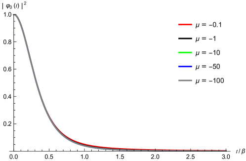
Figure 9: The numerical results of $|\varphi_{0}(t)|^{2}$ in the bosonic case with various chemical potentials as $\mu<0$. The curves are very close to each other.

4.2.3 $\mu<0$

Let’s turn back to the fermionic case with the chemical potential $\mu<0$, the Wightman power spectrum is

$$f^{W}(\omega) =\mathcal{N}(\mu,\beta,5,-1)\frac{\mu-\omega}{2}\frac{1}{\cosh\frac{\beta\omega}{2}}\Theta(\mu-\omega)$$ (103)

$$=\mathcal{N}(\mu,\beta,5,-1)(\mu-\omega)\frac{e^{\beta\omega/2}}{1+e^{\beta\omega}}\Theta(\mu-\omega)$$

$$=\mathcal{N}(\mu,\beta,5,-1)(\mu-\omega)\sum_{k=0}^{\infty}(-1)^{k}e^{\beta\omega(k+1/2)}\Theta(\mu-\omega).$$

From the normalization condition (33), the constant in the above equation (103) can be determined as

$$\mathcal{N}(\mu,\beta,5,-1)=\frac{\pi\beta^{2}e^{-\frac{\beta\mu}{2}}}{2\,_{3}F_{2}\left(\frac{1}{2},\frac{1}{2},1;\frac{3}{2},\frac{3}{2};-e^{\beta\mu}\right)}.$$ (104)

Consequently, the moments $\mu_{n}$ becomes

$$\mu_{n}= \sum_{k=0}^{\infty}\frac{\beta^{2}2^{n-1}e^{-\frac{\beta\mu}{2}}(-1)^{k+n}(2\beta k+\beta)^{-n-2}}{\,{}_{3}F_{2}\left(\frac{1}{2},\frac{1}{2},1;\frac{3}{2},\frac{3}{2};-e^{\beta\mu}\right)}$$ (105)

$${\times}\left(\beta(2k+1)\mu\Gamma\left(n+1,-\frac{1}{2}\beta(2k+1)\mu\right)+2\Gamma\left(n+2,-\frac{1}{2}\beta(2k+1)\mu\right)\right).$$

The resulting Lanczos coefficients $a_{n}$ and $b_{n}$ are exhibited in the Figure 10.

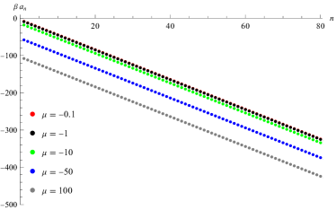
Figure 10: (a) Lanczos coefficients $a_{n}$ in the fermionic case as $\mu<0$.; (b) Lanczos coefficients $b_{n}$ in the fermionic case as $\mu<0$. They overlap together for various chemical potentials.

Chemical potential	$\beta a_{n}$	$\beta b_{n}$
$0$	$-4.011472827-3.999990429n$	$1.004458037+1.999996819n$
$-0.1$	$-4.110594174-3.999991162n$	$1.004020088+1.999997183n$
$-1$	$-5.004915662-3.999995899n$	$1.001191152+1.999999536n$
$-10$	$-14.00000068-3.999999999n$	$0.9987450989+2.000001569n$
$-50$	$-54.00000000-4.000000000n$	$0.9987447602+2.000001569n$
$-100$	$-104.0000000-4.000000000n$	$0.9987447602+2.000001569n$

Table 3: The numerical results of Lanczos coefficients when $\mu\leq 0$ in the fermionic case.

We list the numerical results of the fittings in the Table 3 for the fermionic case. Similar to the bosonic case, the coefficients $a_{n}$ are almost parallel to each other for various chemical potentials, while $b_{n}$ almost overlap together. From the Table 3, the linear relations are roughly,

$$\beta a_{n} \approx -4(n+1)-\mu,$$ (106)

$$\beta b_{n} \approx 2n+1.$$ (107)

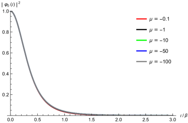
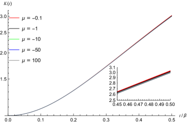
Figure 11: (a) The profile of $|\varphi_{0}(t)|^{2}$ for the fermionic case at different chemical potentials when $\mu<0$; (b) The Krylov complexity for the fermionic case at different chemical potentials when $\mu<0$.

The corresponding $\lvert\varphi_{0}(t)\rvert^{2}$ of the auto-correlation functions and the Krylov complexity are shown in the Figure 11. It is found that $\lvert\varphi_{0}(t)\rvert^{2}$ almost overlap together as well as the Krylov complexities for various chemical potentials. This is consistent with our discussions in the preceding subsection 4.2.2 that if the Lanczos coefficients $b_{n}$ are similar to each other, and $\lvert\varphi_{0}(t)\rvert^{2}$ are also similar, then the Krylov complexities will overlap. However, it is interesting to see that, although the Krylov complexities almost overlap, there are still some minor discrepancies between them. In the inset plot of the Figure 11 we can still distinguish some minor discrepancies between the Krylov complexities for various chemical potentials at late time. From the inset plot we see that unlike in the bosonic case (see Figure 5), the Krylov complexity in the fermionic case is bigger as the chemical potential is greater. In the Table 2, we also present the asymptotic slope of $\log K(t)$ for fermionic case. Unlike the bosonic case, it is interesting to see that in the fermionic case, the smaller the chemical potential is, the smaller the slope will be. And finally they will approach to $2.746$ which is the same as that in the bosonic case.

5 Conclusions

In this paper, we have applied the Krylov subspace method in the grand canonical ensemble to investigate the Krylov complexity of the non-relativistic Schrödinger field with various chemical potentials, especially as the chemical potential is zero or negative. We found that regardless of whether the chemical potential is zero or negative, or whether it is for bosonic or fermionic case, the Lanczos coefficients $\{a_{n}\}$ and $\{b_{n}\}$ are approximately linear and very close to

$$\beta a_{n} \approx -4(n+1)-\mu,$$

$$\beta b_{n} \approx 2n+1.$$

This appears to be somewhat unexpected, as the Wightman power spectrum and the auto-correlation functions are clearly different in various situations. However, they possess similar Lanczos coefficients and consequently exhibit similar behaviors of Krylov complexity. We suspect that there must be some key quantities that is similar between them, and we find that this quantity is the square of the absolute values of auto-correlation function $\lvert\varphi_{0}(t)\rvert^{2}$. That is to say, similar behavior of the $\lvert\varphi_{0}(t)\rvert^{2}$ for bosonic and fermionic cases will yield similar behaviors of the Krylov complexity.

However, in details there are still some discrepancies between the bosonic and fermionic case. We found that at early times, the Krylov complexities for both bosonic and fermionic cases will overlap. However, as time goes by, the Krylov complexity for the bosonic case with a larger chemical potential grows slightly faster than that with a smaller chemical potential. On the contrary, for fermionic case, as time increases the Krylov complexity with a smaller chemical potential grows slightly faster than that with a larger chemical potential. By fitting the slopes of $K(t)$ at late time, we found that for the bosonic case, as the chemical potential decreases, the asymptotic slope increases. However, for the fermionic case, as the chemical potential decreases, the asymptotic slope decreases. Moreover, both in the bosonic and fermionic cases the asymptotic slope will approach $2.746$ for small chemical potentials. It is interesting to see that this slope is smaller than the twice of the slope of $b_{n}$. This is because we are considering the Krylov complexity of non-Hermitian operators, in this case the Lanczos coefficients $a_{n}$ will contribute to the Krylov complexity. We expect that our work will shed light on the study of Krylov complexity of the non-relativistic field theory with non-Hermitian operators.

Appendix A Solve the discrete Schrödinger equation

To solve the discrete Schrödinger equation, we need to first discretize time, letting $t_{i}\approx(i-1)\Delta t,$ where $i=1,2,\ldots$, $\Delta t$ is a small time interval. Then we have

$$\varphi_{n}(t_{i+1}) =\varphi_{n}(t_{i}+\Delta t)$$ (108)

$$\approx\varphi_{n}(t_{i})+\partial_{t}\varphi_{n}(t_{i})\Delta t$$

$$=\varphi_{n}(t_{i})+[b_{n}\varphi_{n-1}(t_{i})-b_{n+1}\varphi_{n+1}(t_{i})+ia_{n}\varphi_{n}(t_{i})]\Delta t.$$

Write $\varphi_{n}(t_{i})$ as $\varphi^{i}_{n}$ and introduce the vector $\vec{\varphi}^{i}=(\varphi^{i}_{0}\ \varphi^{i}_{1}\cdots)^{\text{T}}$, then (108) can be written in a more compact form

$$\vec{\varphi}^{i+1}=\vec{\varphi}^{i}+A\vec{\varphi}^{i}\Delta t,$$ (109)

where $A$ is a matrix

$$A=\left(\begin{matrix}ia_{0}&-b_{1}&0&0&0&\cdots\\ b_{1}&ia_{1}&-b_{2}&0&0&\cdots\\ 0&b_{2}&ia_{2}&-b_{3}&0&\cdots\\ \vdots&\vdots&\vdots&\vdots&\vdots&\ddots\end{matrix}\right).$$ (110)

To utilize the fourth-order Runge-Kutta method, (109) can be rewritten as

$$\vec{\varphi}^{i+1}=\vec{\varphi}^{i}+\frac{\Delta t}{6}(K_{1}+2K_{2}+2K_{3}+K_{4}),$$ (111)

where

$$K_{1}=A\vec{\varphi}^{i},\qquad K_{2}=A(\vec{\varphi}^{i}+K_{1}\Delta t/2),$$ (112)

$$K_{3}=A(\vec{\varphi}^{i}+K_{2}\Delta t/2),\qquad K_{4}=A(\vec{\varphi}^{i}+K_{3}\Delta t).$$ (113)

Once the Lanczos coefficients $\{a_{n}\}$ and $\{b_{n}\}$ are obtained, it is equivalent to knowing the matrix $A$. Knowing $\varphi_{n}(0)$ also means knowing $\vec{\varphi}^{1}$, and from (111), one can calculate $\vec{\varphi}^{i}$.

Appendix B Derive equation (63)

Here, only the bosonic case is considered, and the results for the fermionic case are the same as those for the bosonic case. Define the retarded correlator

$$D^{R}_{ab}(t,\mathbf{x};t^{\prime},\mathbf{x}^{\prime})\equiv i\expectationvalue{\theta(t-t^{\prime})[\phi_{a}(t,\mathbf{x}),\psi_{b}(t^{\prime},\mathbf{x}^{\prime})]}.$$ (114)

Note that

$$\theta(t)=i\int_{-\infty}^{\infty}\frac{d\omega}{2\pi}\frac{e^{-i\omega t}}{\omega+i\epsilon},\qquad\epsilon=0^{+}.$$ (115)

Therefore, in momentum space, we have

$$D^{R}_{ab}(\omega,\mathbf{k})=\int_{-\infty}^{\infty}\frac{d\omega^{\prime}}{2\pi}\frac{\rho_{ab}(\omega^{\prime},\mathbf{k})}{\omega^{\prime}-\omega-i\epsilon}.$$ (116)

Make use of the identity

$$\frac{1}{x\pm i\epsilon}=\mathcal{P}\frac{1}{x}\mp i\pi\delta(x),$$ (117)

we obtain

$$\rho_{ab}(\omega,\mathbf{k})=2\imaginary D^{R}_{ab}(\omega,\mathbf{k}),$$ (118)

where $\mathcal{P}$ denotes the principal value. On the other hand, the relationship between the imaginary-time correlation function, which is also known as the thermal propagator, and the spectral density is

$$\mathcal{D}_{ab}(\omega_{n},\mathbf{k})=\int_{-\infty}^{\infty}\frac{d\omega^{\prime}}{2\pi}\frac{\rho_{ab}(\omega^{\prime},\mathbf{k})}{\omega^{\prime}+i\omega_{n}}.$$ (119)

That is to say, by simply replacing $\omega_{n}$ with $i\omega-\epsilon$, one can obtain the retarded correlation function from the thermal propagator

$$D^{R}_{ab}(\omega,\mathbf{k})=\mathcal{D}_{ab}(\omega_{n}\rightarrow i\omega-\epsilon,\mathbf{k}).$$ (120)

The thermal propagator of Schrödinger field theory is given by (62), then we have

$$\rho_{ab}(\omega,\mathbf{k}) =2\imaginary D^{R}_{ab}(\omega,\mathbf{k})$$ (121)

$$=2\imaginary\mathcal{D}(\omega_{n}\rightarrow i\omega-\epsilon,\mathbf{k})$$

$$=2\Im{\frac{1}{i(i\omega-\epsilon)+\frac{\mathbf{k}^{2}}{2m}-\mu}}$$

$$=2\Im{\frac{1}{\frac{\mathbf{k}^{2}}{2m}-\mu-\omega-i\epsilon}}$$

$$=2\Im{\mathcal{P}\left(\frac{\mathbf{k}^{2}}{2m}-\mu-\omega\right)+i\pi\delta\left(\frac{\mathbf{k}^{2}}{2m}-\mu-\omega\right)}$$

$$=2\pi\delta(\xi_{\mathbf{k}}-\omega).$$

This is the equation (63) in the main text.

References

- (1) D.E. Parker, X. Cao, A. Avdoshkin, T. Scaffidi and E. Altman, A Universal Operator Growth Hypothesis, Phys. Rev. X 9 (2019) 041017 [1812.08657].
- (2) E. Rabinovici, A. Sánchez-Garrido, R. Shir and J. Sonner, Krylov complexity from integrability to chaos, JHEP 07 (2022) 151 [2207.07701].
- (3) C. Liu, H. Tang and H. Zhai, Krylov complexity in open quantum systems, Phys. Rev. Res. 5 (2023) 033085 [2207.13603].
- (4) F.B. Trigueros and C.-J. Lin, Krylov complexity of many-body localization: Operator localization in Krylov basis, SciPost Phys. 13 (2022) 037 [2112.04722].
- (5) B. Bhattacharjee, P. Nandy and T. Pathak, Krylov complexity in large q and double-scaled SYK model, JHEP 08 (2023) 099 [2210.02474].
- (6) P. Caputa, N. Gupta, S.S. Haque, S. Liu, J. Murugan and H.J.R. Van Zyl, Spread complexity and topological transitions in the Kitaev chain, JHEP 01 (2023) 120 [2208.06311].
- (7) B. Bhattacharjee, P. Nandy and T. Pathak, Operator dynamics in Lindbladian SYK: a Krylov complexity perspective, JHEP 01 (2024) 094 [2311.00753].
- (8) B. Craps, O. Evnin and G. Pascuzzi, Multiseed Krylov complexity, 2409.15666.
- (9) H.A. Camargo, V. Jahnke, K.-Y. Kim and M. Nishida, Krylov complexity in free and interacting scalar field theories with bounded power spectrum, JHEP 05 (2023) 226 [2212.14702].
- (10) P.-Z. He and H.-Q. Zhang, Probing Krylov complexity in scalar field theory with general temperatures, JHEP 11 (2024) 014 [2407.02756].
- (11) A. Chattopadhyay, V. Malvimat and A. Mitra, Krylov complexity of deformed conformal field theories, JHEP 08 (2024) 053 [2405.03630].
- (12) V. Malvimat, S. Porey and B. Roy, Krylov Complexity in CFTs with SL deformed Hamiltonians, 2402.15835.
- (13) M.J. Vasli, K. Babaei Velni, M.R. Mohammadi Mozaffar, A. Mollabashi and M. Alishahiha, Krylov complexity in Lifshitz-type scalar field theories, Eur. Phys. J. C 84 (2024) 235 [2307.08307].
- (14) A. Kundu, V. Malvimat and R. Sinha, State dependence of Krylov complexity in 2d CFTs, JHEP 09 (2023) 011 [2303.03426].
- (15) A. Avdoshkin, A. Dymarsky and M. Smolkin, Krylov complexity in quantum field theory, and beyond, JHEP 06 (2024) 066 [2212.14429].
- (16) S. Khetrapal, Chaos and operator growth in 2d CFT, JHEP 03 (2023) 176 [2210.15860].
- (17) K. Adhikari, S. Choudhury and A. Roy, Krylov Complexity in Quantum Field Theory, Nucl. Phys. B 993 (2023) 116263 [2204.02250].
- (18) A. Dymarsky and M. Smolkin, Krylov complexity in conformal field theory, Phys. Rev. D 104 (2021) L081702 [2104.09514].
- (19) E. Rabinovici, A. Sánchez-Garrido, R. Shir and J. Sonner, A bulk manifestation of Krylov complexity, JHEP 08 (2023) 213 [2305.04355].
- (20) A. Kar, L. Lamprou, M. Rozali and J. Sully, Random matrix theory for complexity growth and black hole interiors, JHEP 01 (2022) 016 [2106.02046].
- (21) K. Adhikari and S. Choudhury, Cosmological Krylov Complexity, Fortsch. Phys. 70 (2022) 2200126 [2203.14330].
- (22) T. Li and L.-H. Liu, Krylov complexity of thermal state in early universe, 2408.03293.
- (23) T. Li and L.-H. Liu, Inflationary complexity of thermal state, 2405.01433.
- (24) T. Li and L.-H. Liu, Inflationary Krylov complexity, JHEP 04 (2024) 123 [2401.09307].
- (25) P. Nandy, A.S. Matsoukas-Roubeas, P. Martínez-Azcona, A. Dymarsky and A. del Campo, Quantum Dynamics in Krylov Space: Methods and Applications, 2405.09628.
- (26) K. Hashimoto, K. Murata and R. Yoshii, Out-of-time-order correlators in quantum mechanics, JHEP 10 (2017) 138 [1703.09435].
- (27) M. Srednicki, Chaos and quantum thermalization, Phys. Rev. E 50 (1994) 888.
- (28) A. Piga, M. Lewenstein and J.Q. Quach, Quantum chaos and entanglement in ergodic and nonergodic systems, Phys. Rev. E 99 (2019) 032213.
- (29) A.R. Brown and L. Susskind, Complexity geometry of a single qubit, Phys. Rev. D 100 (2019) 046020.
- (30) C. Lv, R. Zhang and Q. Zhou, Building Krylov complexity from circuit complexity, Phys. Rev. Res. 6 (2024) L042001 [2303.07343].
- (31) V. Balasubramanian, P. Caputa, J.M. Magan and Q. Wu, Quantum chaos and the complexity of spread of states, Phys. Rev. D 106 (2022) 046007 [2202.06957].
- (32) M. Ganguli, Spread Complexity in Non-Hermitian Many-Body Localization Transition, 2411.11347.
- (33) Y. Fu, K.-Y. Kim, K. Pal and K. Pal, Statistics and Complexity of Wavefunction Spreading in Quantum Dynamical Systems, 2411.09390.
- (34) P. Nandy, T. Pathak, Z.-Y. Xian and J. Erdmenger, A Krylov space approach to Singular Value Decomposition in non-Hermitian systems, 2411.09309.
- (35) Z.-Y. Fan, Momentum-Krylov complexity correspondence, 2411.04492.
- (36) J. Xu, On Chord Dynamics and Complexity Growth in Double-Scaled SYK, 2411.04251.
- (37) P. Caputa, B. Chen, R.W. McDonald, J. Simón and B. Strittmatter, Spread Complexity Rate as Proper Momentum, 2410.23334.
- (38) M. Baggioli, K.-B. Huh, H.-S. Jeong, K.-Y. Kim and J.F. Pedraza, Krylov complexity as an order parameter for quantum chaotic-integrable transitions, 2407.17054.
- (39) E. Rabinovici, A. Sánchez-Garrido, R. Shir and J. Sonner, Operator complexity: a journey to the edge of Krylov space, JHEP 06 (2021) 062 [2009.01862].
- (40) B. Bhattacharjee, X. Cao, P. Nandy and T. Pathak, Krylov complexity in saddle-dominated scrambling, JHEP 05 (2022) 174 [2203.03534].
- (41) E. Rabinovici, A. Sánchez-Garrido, R. Shir and J. Sonner, Krylov localization and suppression of complexity, JHEP 03 (2022) 211 [2112.12128].
- (42) P. Caputa and S. Liu, Quantum complexity and topological phases of matter, Phys. Rev. B 106 (2022) 195125 [2205.05688].
- (43) A. Bhattacharya, P. Nandy, P.P. Nath and H. Sahu, On Krylov complexity in open systems: an approach via bi-Lanczos algorithm, JHEP 12 (2023) 066 [2303.04175].
- (44) J. Erdmenger, S.-K. Jian and Z.-Y. Xian, Universal chaotic dynamics from Krylov space, JHEP 08 (2023) 176 [2303.12151].
- (45) B. Bhattacharjee, S. Sur and P. Nandy, Probing quantum scars and weak ergodicity breaking through quantum complexity, Phys. Rev. B 106 (2022) 205150 [2208.05503].
- (46) A. Bhattacharya, P. Nandy, P.P. Nath and H. Sahu, Operator growth and Krylov construction in dissipative open quantum systems, JHEP 12 (2022) 081 [2207.05347].
- (47) B. Bhattacharjee, X. Cao, P. Nandy and T. Pathak, Operator growth in open quantum systems: lessons from the dissipative SYK, JHEP 03 (2023) 054 [2212.06180].
- (48) H.A. Camargo, V. Jahnke, H.-S. Jeong, K.-Y. Kim and M. Nishida, Spectral and Krylov complexity in billiard systems, Phys. Rev. D 109 (2024) 046017 [2306.11632].
- (49) K.-B. Huh, H.-S. Jeong and J.F. Pedraza, Spread complexity in saddle-dominated scrambling, JHEP 05 (2024) 137 [2312.12593].
- (50) H.A. Camargo, K.-B. Huh, V. Jahnke, H.-S. Jeong, K.-Y. Kim and M. Nishida, Spread and spectral complexity in quantum spin chains: from integrability to chaos, JHEP 08 (2024) 241 [2405.11254].
- (51) S. He, P.H.C. Lau, Z.-Y. Xian and L. Zhao, Quantum chaos, scrambling and operator growth in deformed SYK models, JHEP 12 (2022) 070 [2209.14936].
- (52) P. Caputa, H.-S. Jeong, S. Liu, J.F. Pedraza and L.-C. Qu, Krylov complexity of density matrix operators, JHEP 05 (2024) 337 [2402.09522].
- (53) N. Hörnedal, N. Carabba, A.S. Matsoukas-Roubeas and A. del Campo, Ultimate Speed Limits to the Growth of Operator Complexity, Commun. Phys. 5 (2022) 207 [2202.05006].
- (54) P.H.S. Bento, A. del Campo and L.C. Céleri, Krylov complexity and dynamical phase transition in the quenched Lipkin-Meshkov-Glick model, Phys. Rev. B 109 (2024) 224304 [2312.05321].
- (55) S. Nandy, B. Mukherjee, A. Bhattacharyya and A. Banerjee, Quantum state complexity meets many-body scars, J. Phys. Condens. Matter 36 (2024) 155601 [2305.13322].
- (56) A. Dymarsky and A. Gorsky, Quantum chaos as delocalization in Krylov space, Phys. Rev. B 102 (2020) 085137 [1912.12227].
- (57) A. Altland and B.D. Simons, Condensed matter field theory, Cambridge university press (2010).
- (58) E.G. Harris, A pedestrian approach to quantum field theory, Courier Corporation (2014).
- (59) M. Mintchev, D. Pontello, A. Sartori and E. Tonni, Entanglement entropies of an interval in the free Schrödinger field theory at finite density, JHEP 07 (2022) 120 [2201.04522].
- (60) J.J. Sakurai and J. Napolitano, Modern quantum mechanics, Cambridge University Press (2020).
- (61) P. Caputa, J.M. Magan and D. Patramanis, Geometry of Krylov complexity, Phys. Rev. Res. 4 (2022) 013041 [2109.03824].
- (62) R. Geroch, Quantum field theory: 1971 lecture notes, vol. 2, Minkowski Institute Press (2013).
- (63) V. Viswanath and G. Müller, The recursion method: application to many body dynamics, vol. 23, Springer Science & Business Media (1994).
- (64) M.E. Peskin, An introduction to quantum field theory, CRC press (2018).
- (65) J.I. Kapusta and C. Gale, Finite-temperature field theory: Principles and applications, Cambridge university press (2007).