The Mean-Field Survival Model for Stripe Formation in Zebrafish Exhibits Turing Instability

Abstract

Zebrafish have been used as a model organism in many areas of biology, including the study of pattern formation. The mean-field survival model is a coupled ODE system describing the expected evolution of chromatophores coordinating to form stripes in zebrafish. This paper presents analysis of the model focusing on parameters for the number of cells, length of distant-neighbor interactions, and rates related to birth and death of chromatophores. We derive the conditions on these parameters for a Turing bifurcation to occur and show that the model predicts patterns qualitatively similar to those in nature.

In addition to answering questions about this particular model, this paper also serves as a case study for Turing analysis on coupled ODE systems. The qualitative behavior of such coupled ODE models may deviate significantly from continuum limit models. The ability to analyze such systems directly avoids this concern and allows for a more accurate description of the behavior at physically relevant scales.

[Boston University]organization=Department of Mathematics & Statistics, Boston University,addressline=665 Commonweath Ave, city=Boston, postcode=02215, state=MA, country=United States of America

Characterization of Turing instability in a ring-based ODE model for zebrafish.

Quantitative analysis for 4 main parameters, including any finite number of cells, $N$.

Stability curves for large $N$ differ substantially from previous PDE model.

Critical melanophore projection properties similar to those observed in vivo.

Case study for Turing analysis on ring-based ODE models without taking PDE limit.

1 Introduction

The mechanisms by which patterns form is an active area of study in fields ranging from theoretical to lab sciences. The mathematical study of morphogensis was transformed by the discovery of the Turing mechanism in 1952. Turing presented the linear stability analysis (LSA) of various reaction-diffusion models, demonstrating that a differential in diffusion rates can lead to wave-like instabilities and spatially periodic patterns [1]. These models included systems with two or three chemical components, continuous and discrete spatial domains, and analysis on rings and spheres. Much of the mathematical interest in the subject has been on the development of theory for the continuum case [2, 3, 4, 5, 6, 7, 8, 9, 10]. For these conventional reaction-diffusion systems, short-range activation and long-range inhibition is a common mechanism for pattern formation [1, 10]. This terminology refers to the idea that there must be an agent which diffuses slowly and promotes activity and the other agent diffuses quickly and inhibits activity. In models replacing diffusion with a non-local operator, it is possible for pattern formation to occur even when the activator has longer characteristic interaction length than the inhibitor [11]. In discrete models where diffusion is replaced by appropriate coupling terms, similar behavior can occur [1, 12, 13, 14, 15]. In the scenario of networks with the graph Laplacian replacing the continuous Laplacian, multi-stability of stripes and localized patterns has also been observed [12, 13, 14, 15]. Overall, Turing-like instabilities occur in a diverse set of conditions across a large variety of models making them a cornerstone of pattern formation analysis.

This flexibility is particularly applicable to the problem of stripe formation in zebrafish. These stripes are formed by the distribution of pigmented cells, called chromatophores. In zebrafish, there are three primary chromataphores: iridophores (silver), xanthophores (yellow), and melanophores (black). Of these, only iridophores have the mobility to “diffuse” significantly [16, 17, 18, 7, 19, 20, 21]. However, melanophores and xanthophores have been observed to interact with each other in a manner that influences stripe regrowth [22]. Melanophores are capable of extending projections from their cell body which reach multiple cell diameters away. These projections tend to favor movement towards xanthophores and are typically at least three body lengths long [23, 24]. The projections appear to engage in a signaling interaction, leading to a difference in cell birth and death rates after ablation and by extension influence the formation of stripes [22]. Iridophores may not be necessary for stripe formation and have been omitted from many models primarily interested in pattern formation [23, 25, 18, 26]. Readers interested in further review of the state of research into stripe formation in zebrafish specifically will appreciate Kondo, Watanabe, and Miyazawa’s 2021 review article on the subject [27].

In this paper, we study the following model for the interaction of melanophores and xanthophores, derived from the models presented in [25]:

$$X_{j}^{\prime}= 1-X_{j}-M_{j}-X_{j}\left(\tfrac{M_{j-1}+M_{j+1}}{2}\right);$$ (1a)

$$M_{j}^{\prime}= (b+1)(1-X_{j})-(b+d+1)M_{j}-M_{j}\left(\tfrac{X_{j-1}+X_{j+1}}{2}\right)$$

$$+dM_{j}\left(\tfrac{X_{j-h}+X_{j+h}}{2}\right).$$ (1b)

The system consists of $2N$ ODEs for variables $X_{j}$ and $M_{j}$ with $0\leq j\leq N-1$. Cells are modelled on a ring, so indices are modulo $N$. $X_{j}$ and $M_{j}$ represent the probability of finding a xanthophore or melanophore at location $j$ respectively. In equation (1a), the first three terms combined correspond to the probability of location $j$ being empty and a xanthophore appearing with relative rate $1$. The remaining, non-linear term in (1a) represents the death of xanthophores due to the presence of nearby melanophores at relative rate $1$. The first two terms in equation (1b)represents a combination of multiple effects; growth from site $j$ being empty contributes $(b+1)(1-X_{j}-M_{j})$ and natural death contributes $-dM_{j}$. The first of the non-linear terms in (1b) models death from nearby xanthophores while the second models promotion of melanophore growth from xanthophores at distance $h$ away. Short-range interactions, $j\pm 1$, are inhibitory while the long-range interactions, $j\pm h$, are excitatory on melanophores when interacting with xanthophores. Figure 1 contains an example schematic of the overall model structure. The remaining parameters, $b$ and $d$, control the birth rate and death rate of the melanophores respectively. In addition to modelling stripe formation in zebrafish, the model is representative of a variety of cell-compartment models. The analysis of this model is a detailed case study for the analysis of this broad class of models.

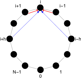
Figure 1: Schematic of ring geometry of model (1). Red arrows represent short-range interactions and blue represent long-range interactions.

This system admits two homogenous equilibria,

$$\left(X,M\right)=\left(1,0\right),\left(\tfrac{d}{b+d},\tfrac{b}{b+2d}\right).$$ (2)

As $X$ and $M$ are probabilities, we restrict the parameter regime to $b\geq 0$ and $d\geq 0$ ($(b,d)\neq(0,0)$) so that these values both remain between $0$ and $1$. While the original model admits all $b\geq-1$, only the $(1,0)$ equilibrium is physically relevant for $-1\leq b<0$. The focus of this paper is on the coexistence equilibrium, which is only physically relevant for $b\geq 0$. Additionally, as the cell locations are on a ring, we restrict the discrete variables to $1\leq h\leq N/2$. Values of $h$ larger than $N/2$ correspond to projections wrapping around the ring and interacting with the same locations as in the $N-h$ case.

1.1 Brief Discussion of Previous Survival Model Analysis

Model (1) is derived by a simple change in notation and some simplifying assumptions from the following model in Konow et al [25].

$$\tfrac{d\langle X_{j}\rangle}{dt}= b_{X}(1-\langle X_{j}\rangle-\langle M_{j}\rangle)-d_{x}\langle X_{j}\rangle-\tfrac{s_{M}}{2}\langle X_{j}\rangle\left(\langle M_{j-1}\rangle+\langle M_{j+1}\rangle\right);$$ (3a)

$$\tfrac{d\langle M_{j}\rangle}{dt}= b_{M}(1-\langle X_{j}\rangle-\langle M_{j}\rangle)-\tfrac{s_{X}}{2}\langle M_{j}\rangle\left(\langle X_{j-1}\rangle+\langle X_{j+1}\rangle\right)$$

$$-\tfrac{d_{MX}}{2}\langle M_{j}\rangle\left(\langle X_{j-h}\rangle+\langle X_{j+h}\rangle\right)$$ (3b)

$$-\tfrac{d_{M}}{2}\langle M_{j}\rangle\left(\langle S_{j-h}\rangle+\langle S_{j+h}\rangle+\langle M_{j-h}\rangle+\langle M_{j+h}\rangle\right).$$

Here, $\langle X_{j}\rangle$ and $\langle M_{j}\rangle$ refer to the expected values of Boolean random variables indicating the presence or absence of xanthophores and melanophores at a given cell location. $b_{X}$ and $b_{M}$ represent birth rates, $d_{x}$ and $d_{M}$ natural death rates, and $s_{x}$ and $s_{M}$ short-range interaction death rates of xanthophores and melanophores respectively. $d_{MX}$ represents a different death rate from melanohphores with a long-range interaction with a xanthophore.

The primary analysis of the model presented in Konow et al. used the simplifying assumptions $s_{x}=s_{M}=1$, $b_{X}=1$, $d_{X}=0$, and $d_{MX}=0$ [25], and these simplifying assumptions are reflected in system (1). We also make a change in notation to simplify many formulas in our results; we define $b=b_{M}-1$, $d=d_{M}$, $X_{j}(t)=\langle X_{j}(t)\rangle$, and $M_{j}(t)=\langle M_{j}(t)\rangle$. Rewriting system (3) using the assumptions and change of notation yields system (1).

Konow et al. presented many results on the numeric and analytic study of three models stripe formation in Zebrafish [25]. Here, we briefly describe how this paper extends their analysis further. The three models in Konow et al. are a continuous-time, discrete-space stochastic model (the survival model), an ODE model (the mean-field survival model) derived from the survival model, and a PDE model (the continuous mean-field survival model) derived from the mean-field survival model. With each successive model, the pattern formation analysis becomes easier, but the behavior is more abstracted from the original model. In their analysis, Konow et al. studied the survival model and the mean-field survival model numerically, while reserving the analytic work for the continuous mean-field survival model [25]. They performed a LSA of the continuous model and characterized the conditions for a Turing bifurcation. This was compared with the onset of pattern formation in the numerical simulations of a variety of scenarios. We build upon this by performing the LSA on the mean-field survival model directly. This provides new information about the original discrete models as well as capturing phenomena which do not appear in the LSA of the continuous mean-field survival model.

1.2 Overview of Objective and Results

The goals of this paper are to characterize the pattern formation properties of model (1) and to demonstrate the benefits of performing LSA on the system of coupled ODEs directly. The results presented in this paper focus on the LSA of the non-trivial homogeneous equilibria from (2) and the spatially periodic patterns that emerge from the Turing instabilities. In particular, we study the bifurcations with respect to four main parameters of (1), including all physically relevant values of the kinetics parameters $b$ and $d$, the population, $N$, and the non-local interaction distance, $h$. All four parameters have significant influences on the stability of the base state (2) and formation of periodic solutions. We analytically determine the dependence of the neutral stability curve on each parameter and identify their individual effects.

Additionally, we study interesting limiting cases and their effect on the bifurcation analysis. The limit $N\to\infty$ provides a valuable point of comparison between the ODE dynamics and the dynamics of the PDE derived in Konow et al for the same limit. The limits for $b$ or $d$ large provide additional information about model (1), such as a simple approximation for the bifurcation curve.

This paper also serves as a case study for the analysis of pattern formation in systems of ODEs in a manner similar to Turing’s original work. This is valuable because often we are interested in models with finite values of $N$ which may significantly deviate from the dynamics of large $N$ PDE limits. In fact, model (1) demonstrates pattern formation for parameters as small as $N=6$ and $h=3$. This type of minimal parameter bound can only be found by analyzing all values of $N$ and $h$ on the ODE system directly.

The results indicate that many of the zebrafish stripe formation trends observed in nature can be explained by signaling between melanophores and distant neighbors. In particular, the width of stripes relative to projection length and minimum typical projection length in the model are the similar to those observed in nature. More generally, this suggests that distant neighbor signaling is a viable mechanism for pattern formation. It also indicates that lattice-based models are capable of accurately describing pattern formation in species where pigment cells are relatively immobile.

2 Results

2.1 Main Results

Let $\left(X_{\text{H}}(t),M_{\text{H}}(t)\right)$ be any homogeneous solution to system (1) and define $u_{j}(t)=X_{j}(t)-X_{\text{H}}(t)$ and $v_{j}(t)=M_{j}(t)-M_{\text{H}}(t)$. Denote the discrete Fourier transform of $u_{j}(t)$ and $v_{j}(t)$ by $\hat{u}_{k}(t)$ and $\hat{v}_{k}(t)$ respectively. Then $\left\{X_{j}(t),M_{j}(t)\right\}_{i=0}^{N-1}$ solves system (1) if and only if $\left\{\hat{u}_{k}(t),\hat{v}_{k}(t)\right\}_{k=0}^{N-1}$ solves system (2.1)

$$\begin{bmatrix}\hat{u}_{k}^{\prime}\\ \hat{v}_{k}^{\prime}\end{bmatrix}= \begin{bmatrix}-M_{\text{H}}(t)-1&-x_{k}X_{\text{H}}(t)-1\\ \left(dT_{h}(x_{k})-x_{k}\right)M_{\text{H}}(t)-b-1&(d-1)X_{\text{H}}(t)-b-d-1\end{bmatrix}\begin{bmatrix}\hat{u}_{k}\\ \hat{v}_{k}\end{bmatrix}$$

$$+\begin{bmatrix}-\big{(}\hat{u}\ast x_{k}\hat{v}\big{)}_{k}\\ -\big{(}x_{k}\hat{u}\ast\hat{v}\big{)}_{k}+d\big{(}T_{h}(x_{k})\hat{u}\ast\hat{v}\big{)}_{k}\end{bmatrix},$$ (4)

where $\ast$ denotes circular convolution on $N$ elements, $x_{k}=\cos\left(2\pi k/N\right)$, and $T_{h}(x)$ is the $h$-order Chebyshev polynomial of the first kind. We will refer to the matrix in equation (2.1) as $\hat{L}_{k}$ and take care that $(X_{\text{H}}(t),M_{\text{H}}(t))$ are clear from context.

For the trivial equilibrium $\left(1,0\right)$, LSA shows that

$$\text{Tr}\left(\hat{L}_{k}\right)= -b-3,$$

$$\text{Det}\left(\hat{L}_{k}\right)= 1-(b+1)x_{k}.$$

For all admissible parameters, $\text{Tr}\left(\hat{L}_{k}\right)<0$. The linear stability is therefore governed entirely by $\text{Det}\left(\hat{L}_{k}\right)$. From this, we conclude the following proposition:

Proposition 1.

The equilibrium $\left(1,0\right)$ is linearly unstable to wave-like perturbations in the subspace of discrete Fourier mode $k$ for each $k$ satisfying

$$x_{k}\geq\tfrac{1}{b+1},$$

and linearly stable to all other perturbations.

For the nontrivial equilibrium $\left(\tfrac{d}{b+d},\tfrac{b}{b+2d}\right)$, the matrix $\hat{L}_{k}$ becomes

$$\hat{L}_{k}= \begin{bmatrix}\frac{-2(b+d)}{b+2d}&\frac{-\left(d(x_{k}+1)+b\right)}{b+d}\\ \frac{b\left(dT_{h}(x_{k})-x_{k}\right)}{b+2d}-(b+1)&\frac{-(b+1)(b+2d)}{b+d}\end{bmatrix}.$$

If $\lambda$ is an eigenvalue of this matrix, then $\vec{\xi}$, defined below, is a corresponding eigenvector.

$$\vec{\xi}= \begin{bmatrix}(b+2d)\left(d(x_{k}+1)+b\right)\\ -\left(2(b+d)^{2}+\lambda\right)\end{bmatrix}.$$

For the values of $b$ and $d$ where this equilibrium is physically reelevant, the first component is strictly positive, but the second component may be positive or negative depending on the value of $\lambda$. From this observation, we conclude the following proposition:

Proposition 2.

If the equilibrium $\left(\tfrac{d}{b+d},\tfrac{b}{b+2d}\right)$ has any center unstable eigenvalues, then the corresponding eigenvectors must have components with opposite signs.

The significance of this proposition, is that it implies that the melanophore and xanthophore stripes are out of phase with each other. This means that, if stripes do form, they will always alternate between high melanophore density and high xanthophore density, as is observed in nature.

To determine whether or not there are such center unstable eigenvalues, we note that

$$\text{Tr}\left(\hat{L}_{k}\right)= \frac{-2(b+d)^{2}-(b+1)(b+2d)^{2}}{(b+d)(b+2d)},$$

$$\text{Det}\left(\hat{L}_{k}\right)= \frac{F\left(x_{k},T_{h}(x_{k}),b,d\right)}{(b+d)(b+2d)},$$

where $F:\mathbb{R}^{4}\to\mathbb{R}$ is defined as follows:

$$F(x,y,b,d)= -bdx^{2}+\left(bd^{2}y-b(b+d)-d(b+1)(b+2d)\right)x$$ (5)

$$+bd(b+d)y+(b+1)(b+d)(b+2d).$$

An alternative characterization of $F$ which will be useful in later analysis is

$$F(x,y,b,d)= b\left(b^{2}+bd(-x+y+3)+d^{2}\left((x+1)y-2(x-1)\right)\right)$$ (6)

$$-(x-1)\left(b^{2}+(x+3)bd+2d^{2}\right).$$

The equilibrium undergoes a Turing bifurcation when $F=0$ with $F>0$ corresponding to linear stability and $F<0$ indicating an instability to appropriate wave-like perturbations. As such, it is important to understand the characteristics of the $F=0$ level set in different planes. Figures 2 and 3 depict different properties of the level set in the $xy$-plane for different choices of $h$, $N$, $b$ and $d$. Figure 4 shows a selection bifurcation curves in the $bd$-plane, formed from segments of $F=0$ level sets for different Fourier modes.

In preparation for the presentation of the main theorems, we define

$$\mathcal{P}=\left\{(b,d)\in\mathbb{R}^{2}:0<d,0<b<d\right\}.$$ (7)

This region will be crucial in the statement of Theorems 1 and 2 classifying the onset of Turing instability with respect to the discrete and continuous parameters respectively. It is important to note that, while these results require $N$ be sufficiently large, this does not mean that the value of $N$ must be exceptionally large. After the presentation of the theorems, we also explore the case of the minimal value of $N$.

To build intuition for the effects of altering each of the four parameters, Figures 2, 3 and 4 show the sets $F=0$ for different parameter values and in different parameter planes. The effect in the $xy$-plane of changing $d$ while $h$ and $N$ are held constant is explored in Figure 2. The effect in the $xy$-plane of changing $h$ and $N$ while $b$ and $d$ are held constant is explored in Figure 3. Finally the effect in the $bd$-plane of changing $h$ and $N$ is explored in Figure 4.

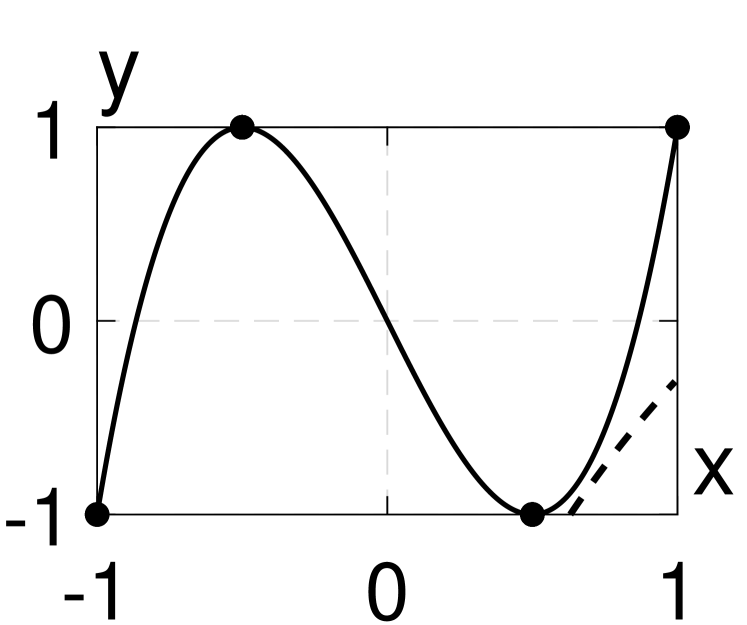
(a)

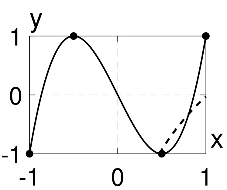
(b)

Figure 2: The curves $y=T_{h}(x)$ (solid black) and $F(x,y,b,d)=0$ (dashed black) in the $xy$-plane. The set with $F<0$ is the region below and to the right of the $F=0$ curve. Turing instability occurs when one or more of the points $(x_{k},T_{h}(x_{k}))$ (black markers) lie in the region with $F<0$ for some $(b,d)$. For both plots, $h=3$ and $N=6$. (2(a)) For $(b,d)=(3,10)$, the equilibrium is linearly stable. (2(b)) For $(b,d)=(3,100)$, the $k=\pm 1$ modes are unstable. Changing the value of $b$ has a similar effect of changing the shape of the $F=0$ curve.

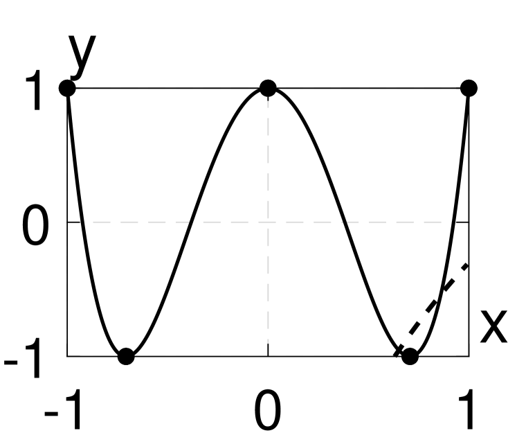
(a)

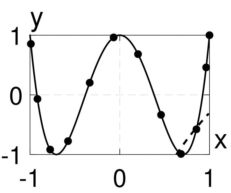
(b)

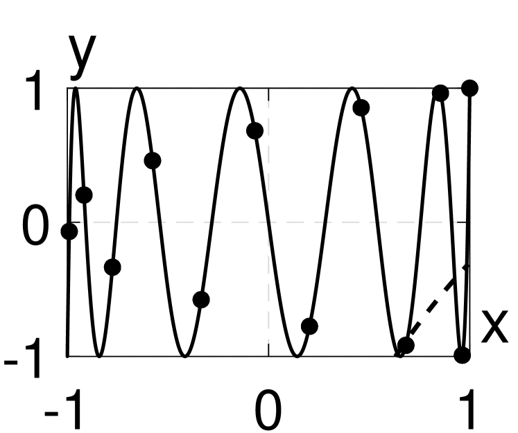
(c)

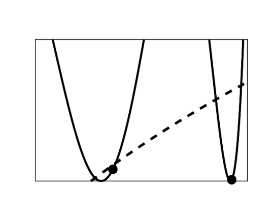
Figure 3: The curves $y=T_{h}(x)$ (solid black) and $F(x,y,b,d)=0$ (dashed black) in the $xy$-plane. The set with $F<0$ is the region below and to the right of the $F=0$ curve. Turing instability occurs when one or more of the points $(x_{k},T_{h}(x_{k}))$ (black markers) lie in the region with $F<0$ for some $(b,d)$. The rightmost marker corresponds to the $k=0$ mode, the next marker corresponds to the $k=\pm 1$ modes, etc. $(b,d)=(3,10)$ for all plots. (3(a)) For $h=4$ and $N=8$, the $k=\pm 1$ modes are unstable. (3(b)) For $h=4$ and $N=23$, the $k=\pm 2,\pm 3$ modes are unstable. Different choices of $(b,d)$ may cause only the $k=\pm 2$ or only the $k=\pm 3$ modes to be unstable. (3(c)) For $h=11$ and $N=23$, the $k=\pm 1,\pm 3$ modes are unstable. Unlike the unstable modes in (3(b)), $k=\pm 3$ modes being unstable implies the $k=\pm 1$ modes are unstable. Inset depicts the region $[1/2,1]\times[-1,0]$.

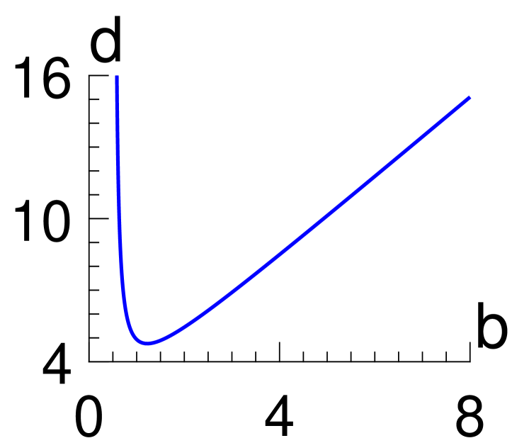
(a)

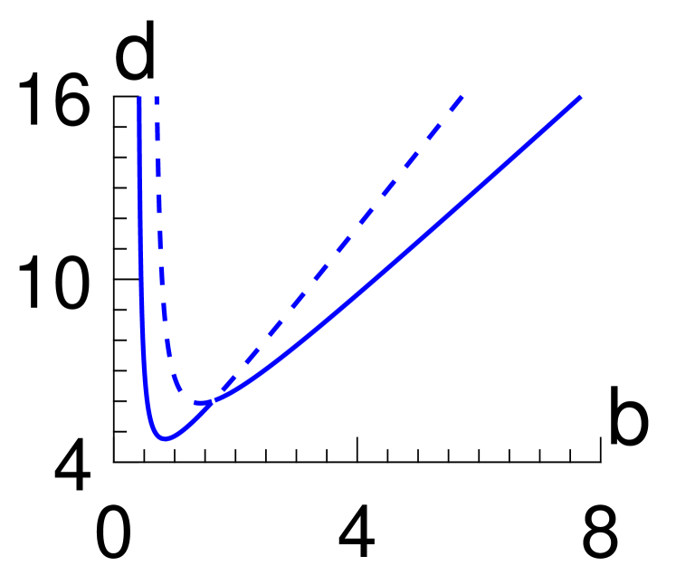
(b)

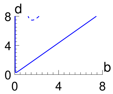
(c)

Figure 4: The curves, $F(x_{k},T_{h}(x_{k}),b,d)=0$, in the $bd$-plane. The bifurcation curve (solid blue) represents the boundary where the equilibrium is neutrally stable. The neutral stability curves (dashed blue) for specific modes represent where the equilibrium is neutrally stable to the given mode, but may already be unstable to other mode(s). For each neutral stability curve, the set with $F<0$ is the set above the curve. (4(a)) For $h=4$ and $N=8$, only the $k=\pm 1$ modes are unstable. (4(b)) For $h=4$ and $N=23$, four modes are unstable. When $b$ is small, the $k=\pm 2$ modes lose stability first, but when $b$ is larger it is the $k=\pm 3$ modes. (4(c)) For $h=11$, and $N=23$, four modes are unstable. The $k=\pm 1$ modes always lose stability before $k=\pm 3$.

Theorem 1.

If $(b,d)\in\mathcal{P}$, then $\exists H_{1}\geq 3$ depending only on $(b,d)$ and $N_{1}\in\mathbb{N}$ depending on $(b,d)$ and $h$ such that $\forall h\geq H_{1}$ and $N\geq N_{1}$, the equilibrium $\left(\tfrac{d}{b+d},\tfrac{b}{b+2d}\right)$ is unstable to appropriate wave-like perturbations in the subspace of discrete Fourier mode(s) $k$ for some $k\neq 0$.

Additionally, $\exists N_{2}\in\mathbb{N}$ depending on $(b,d)$ and $h$ such that $\forall N\geq N_{2}$, the value(s) of $k$ which is most linearly unstable satisfies

$$\left\lceil\tfrac{N}{4h}\right\rceil\leq k\leq\left\lceil\tfrac{N}{2h}\right\rceil,$$ (8)

where $\left\lceil\cdot\right\rceil$ denotes the ceiling function.

If $(b,d)\notin\mathcal{P}$, then the equilibrium $\left(\tfrac{d}{b+d},\tfrac{b}{b+2d}\right)$ is linearly stable.

In summary, for each $(b,d)\in\mathcal{P}$, choosing $h$ and $N$ large enough produces instability to wave-like perturbations. There are also well-defined bounds on the wavelengths of these perturbations based on the ratio of long-range interaction distance to the total number of cell locations. For $(b,d)\notin\mathcal{P}$, there is no such instability. This gives a characterization of the behavior that is expected when $(b,d)$ has already been fixed and $h$ is free to vary. It is also important to consider the behavior when $h$ is fixed and $(b,d)$ is free to vary.

Theorem 2.

$\forall h\geq 3$, $\exists N_{3}\in\mathbb{N}$ depending only on $h$ such that $\forall N\geq N_{3}$, $\exists k\neq 0$ such that the equilibrium $\left(\tfrac{d}{b+d},\tfrac{b}{b+2d}\right)$ is unstable to appropriate wave-like perturbations in the subspace of discrete Fourier mode(s) $k$ and some $(b,d)$. The set of $(b,d)$ for which the $k$ mode is unstable satisfies

$$\mathcal{U}_{k}(h,N)=\left\{(b,d)\in\mathbb{R}_{+}^{2}:F\left(x_{k},T_{h}(x_{k}),b,d\right)<0\right\}\subset\mathcal{P}.$$

For $h=1,2$, the equilibrium is linearly stable for all admissible values of $(b,d)$.

Additionally, $\exists N_{4}\in\mathbb{N}$ depending only on $h$ such that $\forall N\geq N_{4}$, the value(s) of $k$ which first lose stability and/or are the most unstable satisfy

$$\left\lceil\tfrac{N}{4h}\right\rceil\leq k\leq\left\lceil\tfrac{N}{2h}\right\rceil.$$ (9)

The value of $k$ which first loses stability and/or is the most unstable in this scenario depends on $(b,d)$.

In summary, for $h\geq 3$ fixed and $N$ chosen sufficiently large, $(b,d)$ may be chosen to produce a wave-like instability. This is not possible when $h<3$ or $(b,d)\notin\mathcal{P}$. As with Theorem 1, the wavelength of these waves has a well-defined bound. Additionally, the waves that first become unstable may be different for different regions of the $bd$-plane. This provides a description of the behavior when $h$ is fixed and $(b,d)$ is free to vary. Theorems 1 and 2 characterize the onset of instability from two different perspectives by considering different parameters as fixed.

Theorems 1 and 2 both include conditions of $N$ being sufficiently large for the conclusions to hold. For a model with applications for fish of a bounded size, it is important to also consider the question of what is the smallest value of $N$ where instability may occur. This smallest value is $N=6$. The $N$ sufficiently large requirement comes from an argument in the proof involving guaranteeing there is a Fourier mode with $x_{k}$ sufficiently close to the rightmost local minimum of the $T_{h}$ Chebyshev curve. However, for the special case $N=2jh$, then point $x_{\pm j}$ is exactly at the rightmost local minima of the $T_{h}$ Chebyshev curve, as can be seen in Figure 2. This means that for any $j\geq 1$, and $h\geq 3$, $N=2jh$ will be unstable for some $(b,d)$. Combined with the fact that $N\geq 2h$, this means that for model (1), $N=6$ is the absolute minimal case for instability to occur.

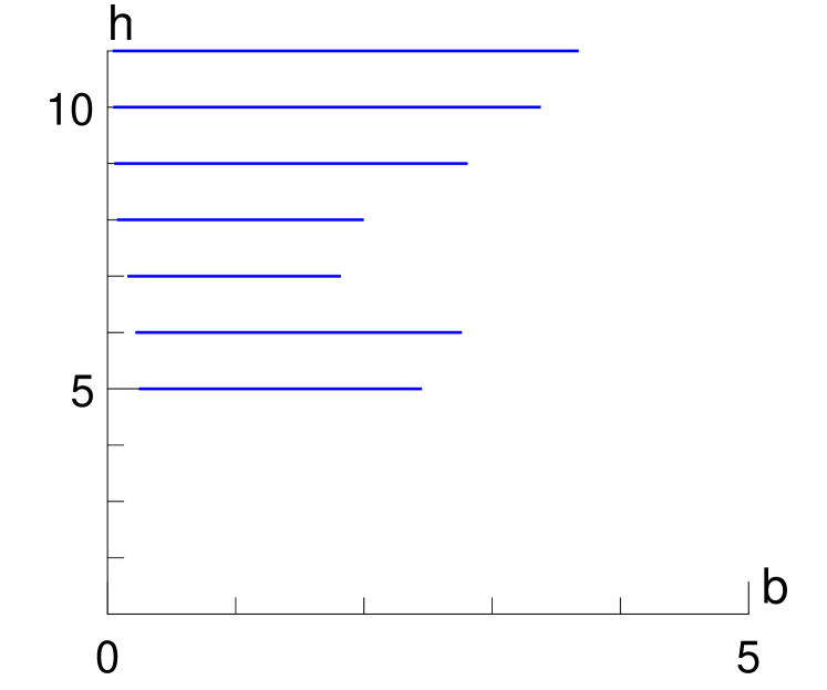
(a)

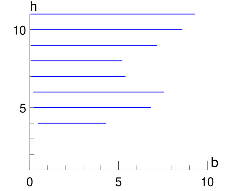
(b)

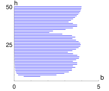
(c)

Figure 5: Regions of linear instability (blue) in the $bh$-plane for fixed $d$ values. In all plots, the left boundary appears to be monotone and approaching $b=0$ as $h$ increases. The right boundary instead has a finely detailed structure that varies with $N$. (5(a)) For $d=4$ and $N=23$, the region of instability satisfies $0\leq b\leq 5$ and $5\leq h$. (5(b)) For $d=10$ and $N=23$, the instability region extends further in the $b$ and $h$ directions than the $d=4$ case. The qualitative shape is still similar. (5(c)) For $d=4$ and $N=100$, the instability region extends further in the $h$ direction. The rich structure of the right boundary demonstrates the value of performing LSA for all values of $h$ and $N$. Analysis of large $N$ continuum limits may fail to capture such details.

The ability to compute linear stability for all combinations of $h$ and $N$ is highlighted in Figure 5. By looking at the regions where the base state is unstable in the $bh$-plane, we see the complicated relationship between the parameters and the stability properties. For $d$ and $N$ fixed, predicting the minimum and maximum $b$ values where Turing instability begins as a function of $h$ is non-trivial. The maximum values in particular vary widely and are neither monotone nor periodic in $h$. Increasing $d$ has the effect of making the instability regions larger, but remaining qualitatively similar. Increasing $N$ increases the complexity of the boundary and makes estimation even less promising. For accurate descriptions of the linear stability of this type of coupled ODE system, it is necessary to perform the analysis for all parameter values, and not just the large $N$ limits.

2.2 Numerical Simulations

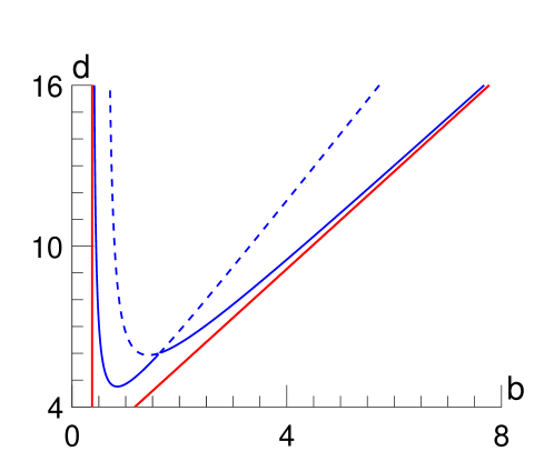
Figure 9: The bifurcation curve (solid blue) and neutral stability curves (dashed blue) for specific modes with $h=4$ and $N=23$. The $k=\pm 2,\pm 3$ neutral stability curves contribute the vertical and slant asymptotes (solid red) respectively.

Using MATLAB’s ode89 program, we can simulate the system and compare the numerical results to the theoretical predictions. All simulations were initialized with random initial data distributed uniformly within a $\pm 0.05$ window of the homogeneous equilibrium. Figures 6 and 7 depict the steady state and time series data respectively of a representative simulation. Figure 8 depicts time series data for a set of parameters values on either side of the bifurcation curve in Figure 9.

Figure 6 depicts the numerical steady state for a simulation with $h=4$, $N=23$, $b=4$, and $d=10$. For these parameter values, the linear stability theory states that there should be instability in the $k=\pm 2,\pm 3$ modes. In parameter space, these values are closer to the neutral stability curve of $k=\pm 2$ than $k=\pm 3$. Heuristically, one may expect the $k=\pm 3$ modes to experience faster exponential growth than the $k=\pm 2$ modes and be more likely to be the dominant mode in the steady state. While non-rigorous, this heuristic does correctly predict the dominant mode. Though not depicted, in all simulations the melanophore expected values exhibited oscillations that were out of phase with the xanthophore, increasing the variation in relative expected abundance of each component.

The Fourier space representation of the solution highlights an important phenomenon in the study of Turing patterns on a coupled ODE system. Because $N$ and the dominant value of $k$ in the steady state are coprime, every mode is a resonant mode of the critical mode. In the presented example, the $k=\pm 6,\pm 9$ are double and triple the dominant mode respectively. The $k=\pm 11$ modes are $4$ times the critical mode when considered mod $23$; explicitly, $\pm 11\equiv 4(\mp 3)\mod 23$. The zig-zag structure in the plot is actually an artifact of the higher resonance modes wrapping around at the boundary due to the periodic nature of the DFT. There is no similar phenomenon in the Fourier space representation of a periodic PDE because there is no way to express the positive modes as negative modes in the way that we can in the discrete case.

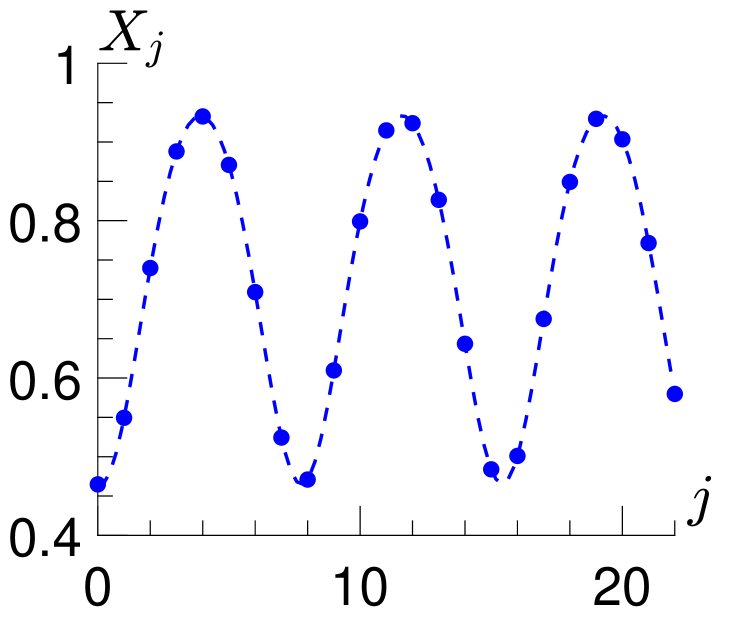
(a)

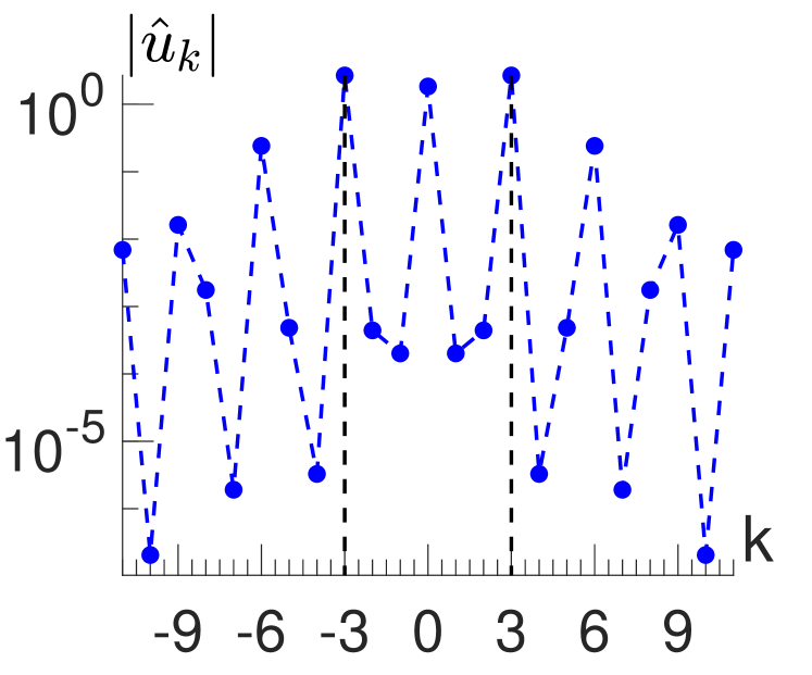
(b)

Figure 6: The numerical steady state for a simulation with parameters $h=4$, $N=23$, $b=4$, and $d=16$. (6(a)) The steady state of the Xanthophore variables (blue dots) and the smooth interpolation of the Fourier spectrum (dashed blue line). (6(b)) The magnitudes of the Fourier space representation of the steady state from (6(a)) expressed as deviation from the homogeneous equilibrium.

In Figure 7, time series data demonstrates the three time regimes where different types of behavior occur. The subfigures depict a short time scale dominated by linear dynamics, an intermediate time dominated by non-linear effects, and a long time dominated by equilibrium stability respectively. The modes $k=0,1,2,3,4,6$ were chosen to be representative of different behaviors amongst different modes. The dominant equilibrium mode is $k=3$, the $k=0,6$ modes are low order resonant modes of the dominant mode, $k=2$ is a high order resonant mode which is also linearly unstable, and modes $k=1,4$ are high order resonance modes of $k=3$ which are also excited by interactions of the $k=2$ and $k=3$ modes.

In the short time, all modes exhibit a short period of fast exponential decay corresponding to the most negative eigenvalue. Then, modes $k=2,3$ experience slow exponential growth from the positive eigenvalues predicted in the LSA. The other modes experience a period of slow exponential decay from the less negative eigenvalues. In the intermediate time, the non-linear coupling causes excitation in the modes which are sums of the unstable modes. The $k=1$ mode is excited by the interaction of the $k=-2$ and $k=3$ modes, for example. In the long time scale, all modes approach constant values. Across simulations, the numerical error near amplitude $10^{-6}$ becomes more significant, even for other ode solvers.

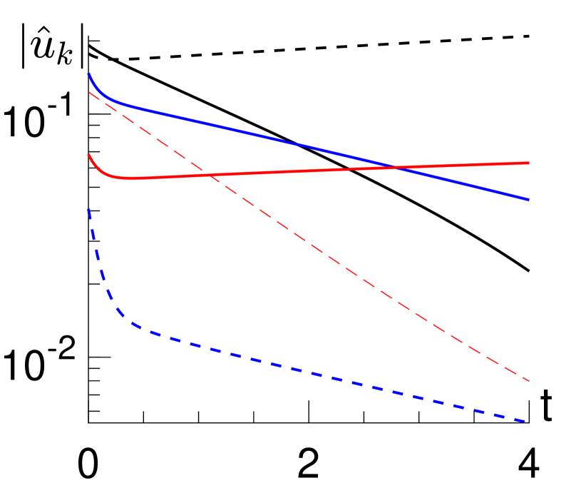
(a)

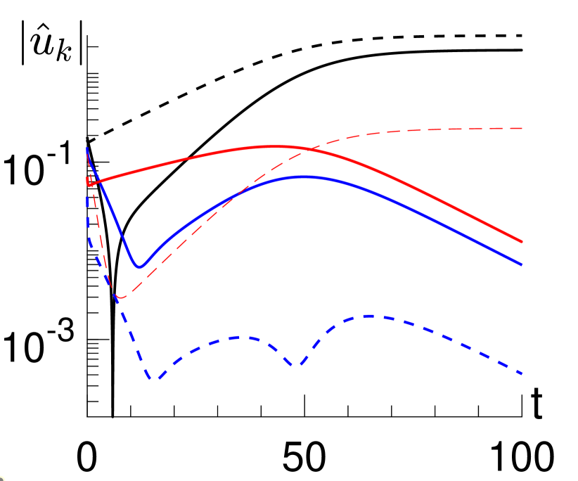
(b)

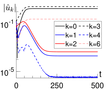
(c)

Figure 7: The time series data of the same simulation as Figure 6 for select Fourier modes on a logarithmic scale. (7(a)) Short-time activity for the selected modes is dominated by the linear dynamics. The $k=2,3$ modes display saddle dynamics while all other modes display sink dynamics. (7(b)) Intermediate-time activity of selected modes displays the effects of non-linear coupling on the transient dynamics. Near $t=50$, the $k=3$ mode is selected as the dominant mode in the steady state. (7(c)) Long-time dynamics are determined by stable steady states. All values are near numerical equilibrium by $t=250$ and do not change significantly by $t=500$.

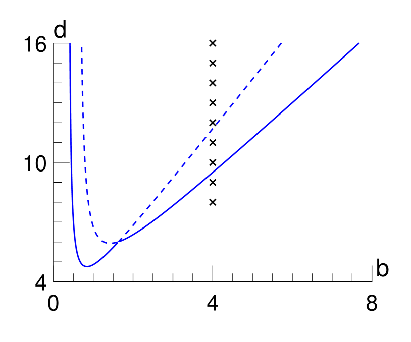
(a)

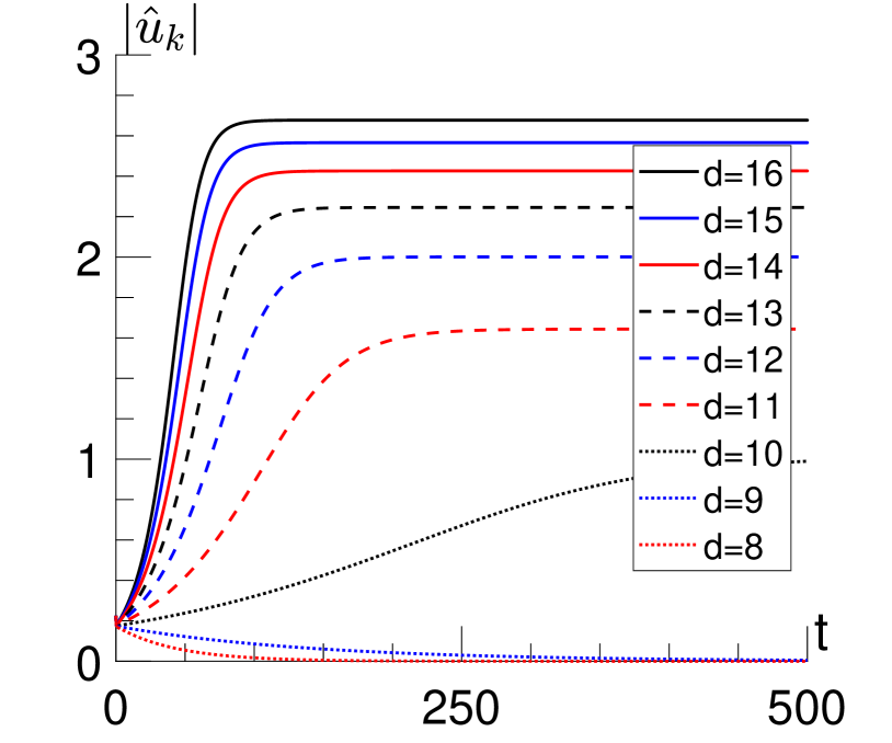
(b)

Figure 8: Time series data for simulations with differing parameter values. For all simulations, $h=4$, $N=23$, and $b=4$. $d$ was sampled between $8$ and $16$ for comparison. In all simulations, the dominant mode at steady state was $k=3$. (8(a)) The selected parameter values (black crosses) relative to the bifurcation curve (solid blue), neutral stability curves (dashed blue) for specific modes and asymptotes (solid red) of the bifurcation curve. (8(b)) Time series data of the dominant modes in the steady state. Parameter values further into the unstable region experience faster exponential growth and larger equilibrium values. Parameter values on the stable side of the bifurcation curve experience exponential decay.

2.3 Other Results

Theorem 3 and Corollary 1 provide results regarding the behavior of the neutral stability curves of individual Fourier modes and bifurcation curves respectively. Namely, these curves approach asymptotes in both directions and the formulas for these asymptotes can be calculated explicitly.

Theorem 3.

For the value(s) of $k$ in Theorem 2 which are unstable, $\mathcal{U}_{k}(h,N)$ is bounded on the left by a vertical asymptote and bounded below and on the right by an oblique asymptote. These asymptotes are characterized by the following equations:

$$b= \frac{2(x_{k}-1)}{f_{2}(x_{k})};$$ (10a)

$$d= \tan(\theta)b+\frac{(x_{k}-1)\left((x_{k}+3)\sin(2\theta)-\cos(2\theta)+3\right)}{2\cos^{2}(\theta)\left(f_{1}(x_{k})\cos(2\theta)+(f_{2}(x_{k})-1)\sin(2\theta)\right)},$$ (10b)

$$2\cot(\theta)= f_{1}(x_{k})+\sqrt{T_{h}^{2}(x_{k})-6x_{k}T_{h}(x_{k})+2T_{h}(x_{k})+(x_{k}+1)^{2}}.$$ (10c)

where $$f_{i}(x)$$ are defined as

$$f_{1}(x)= -x+T_{h}(x)+3,$$

$$f_{2}(x)= (x+1)T_{h}(x)-2(x-1).$$

For all $k$ which are unstable, $\pi/4<\theta<\pi/2$.

Corollary 1.

For $h$ and $N$ satisfying the hypothesis of Theorem 2, the bifurcation curve in the $b,d$-plane, characterized by

$$\partial\left(\bigcup_{k=0}^{N-1}\mathcal{U}_{k}(h,N)\right),$$ (11)

is bounded on the left by a vertical asymptote and eventually bounded below and on the right by an oblique asymptote. These asymptotes are characterized by the following equations:

$$b= \inf_{k}\left(\frac{-2(1-x_{k})}{(x_{k}+1)T_{h}(x_{k})+2(1-x_{k})}\right);$$ (12a)

$$d= \tan(\theta)b+\frac{(x_{k}-1)\left((x_{k}+3)\sin(2\theta)-\cos(2\theta)+3\right)}{2\cos^{2}(\theta)\left(f_{1}(x_{k})\cos(2\theta)+(f_{2}(x_{k})-1)\sin(2\theta)\right)},$$ (12b)

$$2\cot(\theta)= \sup_{k}\left(f_{1}(x_{k})+\sqrt{T_{h}^{2}(x_{k})-6x_{k}T_{h}(x_{k})+2T_{h}(x_{k})+(x_{k}+1)^{2}}\right).$$ (12c)

where the infimum and supremum are taken over the values of $$k$$ which are unstable from Theorem 2.

In short, the neutral stability curve for each Fourier mode has a vertical and slant asymptote. The vertical asymptote is always positive, but the asymptote becomes arbitrarily large for $N$ large and some $k$. The slope of the slant asymptote is always larger that $1$ and becomes arbitrarily large under similar conditions. The asymptotes for the overall bifurcation curve are found by considering the extremal cases of the asymptotes for the individual Fourier modes. For the vertical asymptote, this is the asymptote with the minimal intercept. For the slant asymptote, this is the asymptote with the minimal slope.

We now present results analogous to Theorems 1, 2, and 3 and Corollary 1 which consider a particular limit as $N\to\infty$. The results in these theorems persist as $N\to\infty$ so long as $k/N$ approaches a constant. This corresponds to approaching a fixed wavelength of stripes, rather than a fixed number of stripes. There is linear instability that arises from varying $h$, $b$, and $d$ in similar ways as the main theorems and asymptotes in the $bd$-plane following similar formulas.

Corollary 2.

If $(b,d)\in\mathcal{P}$, then $\forall h\geq H_{1}$, $\exists I\subset\left(1/4h,1/2h\right)$ depending on $(b,d)$ and $h$ such that $\forall\phi\in I$

$$\lim_{N\to\infty,k/N\to\phi}F(x_{k},T_{h}(x_{k}),b,d)<0.$$ (13)

If $(b,d)\notin\mathcal{P}$, then

$$\lim_{N\to\infty,k/N\to\phi}F(x_{k},T_{h}(x_{k}),b,d)\geq 0.$$ (14)

Corollary 3.

Let $\mathcal{U}_{\phi}(h)=\left\{(b,d)\in\mathbb{R}_{+}^{2}:F(x_{\phi},T_{h}(x_{\phi}),b,d)<0\right\}$ where $x_{\phi}=\cos\left(2\pi\phi\right)$. $\forall h\geq 3$, $\exists I\subset\left(1/4h,1/2h\right)$ depending only on $h$ such that $\forall\phi\in I$,

$$\mathcal{U}_{\phi}(h)=\lim_{N\to\infty,k/N\to\phi}\mathcal{U}_{k}(h,N),$$ (15)

and the set is non-empty.

Corollary 4.

$\forall\phi\in I$ as defined in Theorem 3, the set $\mathcal{U}_{\phi}(h)$ is a convex set bounded on the left by a vertical asymptote and bounded below and on the right by an oblique asymptote. These asymptotes are characterized by the equations:

$$b= \frac{-2(1-x_{\phi})}{(x_{\phi}+1)T_{h}(x_{\phi})+2(1-x_{\phi})};$$ (16a)

$$b= \frac{B_{1}}{2}d+C,$$ (16b)

$$C= \frac{B_{1}x_{\phi}+(B_{1}^{2}+4B_{1}+8)x_{\phi}-B_{1}^{2}-6B_{1}-8}{4x_{\phi}T_{h}(x_{\phi})-4(B_{1}+2)x_{\phi}+4(B_{1}+1)T_{h}(x_{\phi})+3B_{1}^{2}+12B_{1}+8},$$ (16c)

$$B_{1}= f_{1}(x_{\phi})+\sqrt{T_{h}(x_{\phi})^{2}-6x_{\phi}T_{h}(x_{\phi})+2T_{h}(x_{\phi})+(x_{\phi}+1)^{2}}.$$ (16d)

Corollary 5.

For $h$ satisfying the hypothesis of Theorem 3, the bifurcation curve in the $b,d$-plane, characterized by

$$\partial\left(\bigcup_{\phi\in I}\mathcal{U}_{\phi}(h)\right),$$ (17)

is bounded on the left by a vertical asymptote and eventually bounded below and on the right by an oblique asymptote. These asymptotes are characterized by the following equations:

$$b= \inf_{\phi\in I}\left(\frac{-2(1-x_{\phi})}{(x_{\phi}+1)T_{h}(x_{\phi})+2(1-x_{\phi})}\right);$$ (18a)

$$b= \frac{B_{*}}{2}d+C,$$ (18b)

$$C= \frac{B_{*}x_{\phi}+(B_{*}^{2}+4B_{*}+8)x_{\phi}-B_{*}^{2}-6B_{*}-8}{4x_{\phi}T_{h}(x_{\phi})-4(B_{*}+2)x_{\phi}+4(B_{*}+1)T_{h}(x_{\phi})+3B_{*}^{2}+12B_{*}+8},$$ (18c)

$$B_{*}= \sup_{\phi\in I}\left(f_{1}(x_{\phi})+\sqrt{T_{h}(x_{\phi})^{2}-6x_{\phi}T_{h}(x_{\phi})+2T_{h}(x_{\phi})+(x_{\phi}+1)^{2}}\right).$$ (18d)

The proof of these results follows a very similar argument to those of the non-limiting analogues. As such, the proofs of these results are deferred to the appendix.

3 Proofs of Main Results

To prove the main results, we make use of the following lemma regarding useful properties of the function $F$:

Lemma 1.

$F$ has the following properties:

• $\forall(b,d)\in\mathcal{P}$, the set $\mathcal{R}(b,d)=\left\{(x,y)\in[-1,1]^{2}:F(x,y,b,d)<0\right\}$ is a neighborhood of $(1,-1)$ contained in the region defined by

  $$\left(1-\frac{b(b+2d)(d-b)}{b^{2}d+3bd^{2}+b^{2}+3bd+2d^{2}},1\right]\times\left[-1,-b/d\right) \subseteq(0,1]\times[-1,0).$$ (19)

• $\forall(b,d)\in\mathcal{P}$, the set $\left\{x\in\mathbb{R}:F(x,-1,b,d)<0\right\}$ contains the interval $(L,1]$ where

  $$L= \frac{b^{3}+2b^{2}d+bd^{2}+b^{2}+4bd+2d^{2}}{b^{2}d+3bd^{2}+b^{2}+4bd+2d^{2}}.$$ (20)

  The infimum of $L$ over the set $\mathcal{P}$ is $1/3$.

• $\forall C\leq 0$ the level sets $F(x,y,b,d)=C$ in $[-1,1]^{2}$ can be expressed with $y$ a concave down, increasing function of $x$.

• $\forall(b,d)\notin\mathcal{P}$, $\mathcal{R}(b,d)=\emptyset$.

The region bounding $\mathcal{R}(b,d)$ has the alternative characterization

$$\left(\frac{b(b+d)^{2}+(b+d)(b+2d)}{b^{2}d+3bd^{2}+b^{2}+3bd+2d^{2}},1\right]\times\left[-1,-b/d\right)\subseteq(0,1]\times[-1,0).$$

These two equivalent characterizations emphasize that the lower bound in the $x$-direction is strictly between $0$ and $1$ for all $(b,d)\in\mathcal{P}$. The bounding region is therefore both non-empty and contained in the set $(0,1]\times[-1,0)$. Proof of this lemma is technical and reserved for the appendix. We can now prove Theorems 1 and 2.

Proof of Theorem 1.

Recall that the Jacobian matrix of the linearization around this equilibrium has

$$\text{Tr}\left(\hat{L}_{k}\right)= \frac{-2(b+d)^{2}-(b+1)(b+2d)^{2}}{(b+d)(b+2d)},$$

$$\text{Det}\left(\hat{L}_{k}\right)= \frac{F\left(x_{k},T_{h}(x_{k}),b,d\right)}{(b+d)(b+2d)},$$

for all modes $k\in\left\{0,...,N-1\right\}$. For admissible values of $(b,d)$, $\text{Tr}\left(\hat{L}_{k}\right)<0$ and $\text{Det}\left(\hat{L}_{k}\right)$ has the same sign as $F\left(x_{k},T_{h}(x_{k}),b,d\right)$. So, there is linear instability if and only if $\exists k$ with $F\left(x_{k},T_{h}(x_{k}),b,d\right)<0$. By Lemma 1, the set $\mathcal{R}(b,d)$ for which $F(x,y,b,d)<0$ is non-empty exactly when $(b,d)\in\mathcal{P}$. Therefore, we may conclude that $(b,d)\notin\mathcal{P}$ implies that the equilibrium is completely linearly stable. This establishes the last statement of the theorem.

To show the other results in the theorem, we first characterize when $F(x,T_{h}(x),b,d)<0$ for $(b,d)\in\mathcal{P}$. For this, we utilize properties of Chebyshev polynomials of the first kind.

• The roots of $T_{h}(x)$ occur at $x=\cos\left(\pi(j+1/2)/h\right)$ for $j\in\left\{0,...,h-1\right\}$ and these roots are simple.

• The local extrema of $T_{h}(x)$ occur at $x=\cos\left(\pi j/h\right)$ for $j\in\left\{1,...,h-1\right\}$.

• All local maxima of $T_{h}(x)$ have value $1$. All local minima of $T_{h}(x)$ have value $-1$.

• $T_{h}(1)=1$.

The rightmost local minimum is $x=\cos\left(\pi/h\right)$. By taking $h$ sufficiently large, this local minimum can be made arbitrarily close to $x=1$. For any fixed $(b,d)\in\mathcal{P}$, the set $\mathcal{R}(b,d)$ contains some open rectangle $(1-\epsilon,1]\times[-1,-1+\delta)$. For $h$ sufficiently large, the local minimum $\left(\cos\left(\pi/h\right),-1\right)$ will be inside of this rectangle, guaranteeing that $F(x,T_{h}(x),b,d)<0$ on some open interval of $x$ values containing $\cos\left(\pi/h\right)$. The fact that $\mathcal{R}(b,d)\subseteq(0,1]\times[-1,0)$ also indicates this open interval is a subset of $\left(\cos\left(3\pi/2h\right),\cos\left(\pi/2h\right)\right)$. We have now established that there exists an $H_{1}\in\mathbb{N}$ such that $h\geq H_{1}$ are all sufficiently large for $F(x,T_{h}(x),b,d)$ to be negative on some open interval of $x$ values. The existence of this interval is necessary but not sufficient for linear instability.

The final step to demonstrating linear instability is to characterize when the intervals where $F(x,T_{h}(x),b,d)<0$ contain points $x_{k}$ for some $k\in\left\{0,...,N-1\right\}$. Recalling that $x_{k}=\cos\left(2\pi k/N\right)$, we derive the following bound on $\lvert x_{k}-x_{k+1}\rvert$:

$$\lvert x_{k}-x_{k+1}\rvert= \left\lvert\cos\left(2\pi k/N\right)-\cos\left(2\pi k+1/N\right)\right\rvert$$

$$= \left\lvert-2\sin\left(\frac{2\pi k/N+2\pi k+1/N}{2}\right)\sin\left(\frac{2\pi k/N-2\pi k+1/N}{2}\right)\right\rvert$$

$$= \left\lvert 2\sin\left(2\pi k/N+\pi/N\right)\sin\left(\pi/N\right)\right\rvert$$

$$\leq 2\sin\left(\pi/N\right)$$

Thus, by also making $N$ sufficiently large, we are able to make $\lvert x_{k}-x_{k+1}\rvert$ arbitrarily small. For any $(b,d)\in\mathcal{P}$ fixed and $h$ sufficiently large, we can then choose $N$ sufficiently large that $\lvert x_{k}-x_{k+1}\rvert$ is smaller than the length of the interval of $x$ values where $F(x,T_{h}(x),b,d)<0$. We then know that $\exists k$ such that $F(x_{k},T_{h}(x_{k}),b,d)<0$ and conclude linear instability to appropriate perturbations. We can rule out the case $k=0$ using the fact that $T_{h}(1)=1$ and $F(1,1,b,d)>0$. This establishes the fact that the equilibrium is unstable to some wave-like perturbations under appropriate conditions.

The characterization of the most linearly unstable waves makes use of the result from Lemma 1 which states the level sets $F=C$ for $C\leq 0$ are concave down and increasing in $x$. Because $y=T_{h}(x)$ have all local minima equal to the global minima on $[-1,1]$, any line connecting the rightmost local minima to any point on $y=T_{h}(x)$ left of the local minima must be non-increasing. So, the rightmost local minima must be on a more negative level set than any point on the curve to the left. We also know $F(x,y,b,d)>0$ for $y>0$ so all points on the curve $y=T_{h}(x)$ right of the rightmost root must also be positive. So, the global minimum of $F(x,T_{h}(x),b,d)$ must be between the rightmost local minimum and rightmost root of $T_{h}(x)$. By taking $N$ sufficiently large, $x_{k}$ can be guaranteed to exist in the interval of values where $F(x_{k},T_{h}(x_{k}),b,d)<F\left(\cos\left(\pi/h\right)),-1,b,d\right)$. Clearly, the value of $F$ at any such $x_{k}$ values is less than those of any $x_{k}$ not in this interval. This interval is guaranteed to be inside of the interval between the rightmost local minimum and rightmost root, $\left(\cos\left(\pi/h\right),\cos\left(\pi/2h\right)\right)$. The bounds in terms of $k$ follow from the definition of $x_{k}$ and appropriate rounding. This establishes the bounds on the most unstable values of $k$ and concludes the proof. ∎

We include the first mode with $x_{k}$ left of $\cos\left(\pi/h\right)$ in the theorem, but this may be excluded by taking $N$ to be sufficiently large. We do not include the first mode with $x_{k}$ right of $\cos\left(\pi/2h\right)$ because we know that $T_{h}(x)>0$ implies $F>0$ and are primarily interested in studying the most unstable mode in scenarios where there is at least one unstable mode.

The proof of Theorem 2 makes use of many of the properties of $F(x,T_{h}(x),b,d)$ and density arguments demonstrated in the proof of Theorem 1.

Proof of Theorem 2.

For $h\geq 3$, the rightmost local minimum of $T_{h}(x)$, located at $x=\cos\left(\pi/h\right)$, is greater than $1/3$. By the established properties of $\mathcal{R}(b,d)$ in Lemma 1, $\left\{x\in\mathbb{R}:F(x,-1,b,d)<0\right\}$ contains an interval $(L,1]$ and $\inf_{(b,d)\in\mathcal{P}}L=1/3$. Therefore, for $h\geq 3$, $F(\cos\left(\pi/h\right),-1,b,d)<0$ for some set of $(b,d)$ values. We now use this to prove the existence of some $N_{3}$ with the desired properties via a proof by contradiction. We desire that $N\geq N_{3}$ guarantee the existence of some admissible $(b,d)$ such that $F(x_{k},T_{h}(x_{k}),b,d)<0$ for some $k\neq 0$. For the sake of contradiction, we assume no such $N_{3}$ exists; $\forall M\in\mathbb{N}$, $\exists N\geq M$ such that $\forall(b,d)$ which are admissible and $\forall k$, $F(x_{k},T_{h}(x_{k}),b,d)\geq 0$. Therefore, for any admissible $(b,d)$, we can construct an increasing sequence $(N_{j})_{j=0}^{\infty}$ such that $N_{j}\to\infty$ and $\min_{k}\left\{F(x_{k},T_{h}(x_{k}),b,d)\right\}\geq 0$. Now, consider the sequence $(k_{j})_{j=0}^{\infty}$ defined by $k_{j}=\left\lceil N_{j}/2h\right\rceil$. As $j\to\infty$, $2\pi k_{j}/N_{j}\to\pi/h$. By the continuity of $F$, $F(x_{k_{j}},T_{h}(x_{k_{j}}),b,d)\to F(\cos\left(\pi/h\right),-1,b,d)$. Clearly, this also implies $\limsup\left(\min_{k}\left\{F(x_{k},T_{h}(x_{k}),b,d)\right\}\right)_{j}$ is bounded above by $F(\cos\left(\pi/h\right),-1,b,d)$. We have already established that we may choose $(b,d)$ such that $F(\cos\left(\pi/h\right),-1,b,d)<0$ so we have a contradiction. There are some $(b,d)$ for which $\exists M(b,d)\in\mathbb{N}$ with $N\geq M(b,d)$ implying $F(x_{k},T_{h}(x_{k}),b,d)<0$ for some $k$, so $N_{3}=M(b,d)$ satisfies the theorem for any such $(b,d)$. The stability of the equilibrium is entirely determined by the sign of $F$ so this establishes the existence of $N_{3}$ such that there is a bifurcation with respect to the continuous parameters resulting in a loss of stability.

The bounds on which modes are the most unstable and/or the first to lose stability follow from the same argument as the proof of Theorem 1. By taking $N$ sufficiently large, it is clear that the least stable mode must be in the specified range because the minimum along the curve $y=T_{h}(x)$ is in the specified range. The argument from the previous proof holds for all non-positive level sets. The question of the first mode to lose stability is simply the question of the least stable mode when that mode lies on the $F=0$ level set. This establishes the bound on the most unstable mode and concludes the proof. ∎

4 Discussion & Conclusions

We have shown that model (1) exhibits Turing instability and derived explicit formulas for the parameter regime in $\mathbb{R}^{2}\times\mathbb{N}^{2}$ where this occurs. According to Theorem 1, choosing $(b,d)\in\mathcal{P}$, see (7), guarantees that for $h$ and $N$ large enough, the homogeneous steady state becomes unstable to spatially periodic perturbations. Similarly, for all $h\geq 3$ and $N$ sufficiently large, Theorem 2 states there are sets of $(b,d)\in\mathcal{P}$ where periodic patterns emerge. In addition to these results for $N$ sufficiently large, we also established that the minimum case for pattern formation in the model is $N=6$ with $h=3$.

The behavior of the survival model bears interesting similarities to lab observations. In particular, Hamada et al [24] observed that the long projections of melanophores were “often greater than three times the length of the cell body and nearly half of the width of stripes”. In model (1), $h\geq 3$ is a necessary condition for stripe formation. Additionally, the condition that $h$ be exactly half of the width of a stripe implies that $k=N/2h$. If $k<N/2h$, then $h$ will be less than half of the width of a stripe. The bounds on $k$ in Theorems 1 and 2 imply that this is always the case for $N$ sufficiently large. Additionally, the analysis shows that the unstable mode with $k$ closest is to $N/2h$ is the mode which produces the slant asymptote. This means that the regime where $b\lesssim d$ is the regime that best matches this physical observation.

Mature wild-type zebrafish most commonly have four black stripes on each side of their body, indicating $k=8$ is a particularly relevant mode to study. The linear stability analysis provides bounds, (8) and (9), on which modes may be unstable. These bounds imply that, for $k=8$ to be unstable, it must be that $14<N/h\leq 32$. For $h=3$ or $h=4$, this corresponds to $42<N\leq 96$ and $56<N\leq 128$ respectively.

These results may also be used to predict changes in pattern as a zebrafish grows. Domain growth is known to effect the development of patterns and should not be dismissed entirely. However, we may use the linear stability results as a first approximation of the true stability properties on a growing fish. The results indicate the number of stripes that are favored should grow proportional to the circumference of the fish in an approximately linear fashion. Existing data supports the idea of linear growth of stripe count relative to standard length [28]. Under the assumption that the circumference is proportional to standard length, this would also imply a linear relationship between stripe count and circumference. Without detailed data on fish circumferences or number of cells in a fish cross section, more concrete comparisons are difficult.

More generally, models which use a distant neighbor signaling interaction as a mechanism for pattern formation may follow similar trends with regards to changing the animal size. Stripe width will likely remain approximately constant while stripe count will grow. Species which demonstrate similar trends may be reasonably modelled in a similar way. Alternatively, species which are observed to have stripes which grow significantly with animal size likely cannot be modelled by this type of distant neighbor interaction or must incorporate other mechanisms.

The parameter regimes where the homogeneous steady state is unstable have explicitly defined asymptotes which bound the behavior for $(b,d)$ large. Combined with numerical calculation, this gives an effective means of approximating the linear stability properties of the system for any parameter values. We also discovered analytic bounds on the possible wavenumbers of the final pattern and may use the linear stability results as a heuristic for predicting the observed wavenumbers.

Finally, the results for $N\to\infty$ provide tools for approximating behavior for $N$ large and assess the validity of continuum models. Konow et al also proposed a PDE model as a first approximation of the mean-field survival model in a continuum limit. The LSA of this PDE model predicts significantly different behavior than the large $N$ limit of the ODE model. For example, in the $bh$-plane, the PDE analysis predicts that the neutral stability curve will resemble a hyperbola with vertical and horizontal asymptotes and that all parameter values above the curve will be unstable [25]. The left boundary is qualitatively similar to the ODE model, but the right bound is significantly different. The region of instability in the ODE model is bounded in the $b$ direction by an intricate curve while the PDE model is not bounded at all. This suggests that the PDE model may only be applicable in a limited region of parameter space or that a different continuum model may more accurately approximate the ODE system. Even in contexts where one desires to study a continuum limit, performing the analysis in the discrete case can still help inform the expected properties of continuum model.

There is still work to be done regarding the survival model. Future efforts may be directed towards analyzing the full generality of parameters in the original survival model. The effects of the other parameters may significantly change the parameter regimes in which stripes form or the wavelength of stripes which are selected. There is also potential for interesting work on the selection mechanism when multiple modes are unstable simultaneously. In numerical simulations with small amplitude, uniformly distributed noise, we see that for some parameter values only one mode is ever selected, while for other parameter values multiples modes may be selected with approximately equal likelihood depending on the initial noise.

Appendix A Proofs of some intermediate results and Theorem 3

Proof of Lemma 1.

Recall the definition of $F$ given below

$$F(x,y,b,d)= -bdx^{2}+\left(bd^{2}y-b(b+d)-d(b+1)(b+2d)\right)x$$

$$+bd(b+d)y+(b+1)(b+d)(b+2d)$$

We begin by computing a collection of derivatives of $F$.

$$\frac{\partial F(x,y,b,d)}{\partial y}= bd^{2}x+bd(b+d)$$

$$= bd(dx+b+d)$$

$$\frac{\partial F(x,y,b,d)}{\partial x}= -2bdx+bd^{2}y-b(b+d)-d(b+1)(b+2d)$$

$$\frac{\partial^{2}F(x,y,b,d)}{\partial x^{2}}= -2bd$$

We will first show that the set $\mathcal{R}(b,d)=\left\{(x,y)\in[-1,1]^{2}:F(x,y,b,d)<0\right\}$ is empty for $(b,d)\notin\mathcal{P}$ and contained in the prescribed region for $(b,d)\in\mathcal{P}$. To do this, we compute $F(1,y,b,d)$, $F(-1,-1,b,d)$, $F(1,-1,b,d)$, and $F(0,-1,b,d)$.

$$F(1,y,b,d)= -bd+bd^{2}y-b(b+d)-d(b+1)(b+2d)+bd(b+d)y$$

$$+(b+1)(b+d)(b+2d)$$

$$= bd(b+2d)y-b(b+2d)+b(b+1)(b+2d)$$

$$= b(b+2d)(dy+b)$$

$$F(-1,-1,b,d)= -bd+bd^{2}+b(b+d)+d(b+1)(b+2d)-bd(b+d)$$

$$+(b+1)(b+d)(b+2d)$$

$$= bd(d-1)-b(b+d)(d-1)+(b+1)(b+2d)^{2}$$

$$= -b^{2}(d-1)+(b+1)(b+2d)^{2}$$

$$= b^{2}-b^{2}d+b^{3}+4b^{2}d+4bd^{2}+b^{2}+4bd+4d^{2}$$

$$= b^{3}+3b^{2}d+4bd^{2}+2b^{2}+4bd+4d^{2}$$

$$F(1,-1,b,d)= b(b+2d)(b-d)$$

$$F(0,-1,b,d)= -bd(b+d)+(b+1)(b+d)(b+2d)$$

$$= b(b+d)^{2}+(b+d)(b+2d)$$

For the admitted values of $(b,d)$ and $x$, $0<b^{2}d\leq\frac{\partial F(x,y,b,d)}{\partial y}$ and $\frac{\partial^{2}F(x,y,b,d)}{\partial x^{2}}<0$. The concavity in $x$ means the set $\left\{x\in\mathbb{R}:F(x,y,b,d)\geq 0\right\}$ is a single closed interval for all fixed $y$. Using the values of $F(-1,-1,b,d)$ and $F(0,-1,b,d)$, we know that the closed interval for $y=-1$ contains $[-1,0]$. Because $F$ is strictly increasing in $y$, we can conclude that for any $y$ these closed intervals where $F\geq 0$ contain $[-1,0]$. These closed intervals will contain all of $[-1,1]$ in the $x$ direction if and only if $F(1,y,b,d)\geq 0$. The formula for $F(1,y,b,d)$ shows this occurs exactly when $y\geq-b/d$. This set of $y$ values contains the entire interval $[-1,1]$ if and only if $(b,d)\notin\mathcal{P}$. The set $\mathcal{R}(b,d)$ is the complement in $[-1,1]^{2}$ of $\bigcup_{y\in[-1,1]}\left\{x\in\mathbb{R}:F(x,y,b,d)\geq 0\right\}$, so $\mathcal{R}(b,d)$ is empty if and only if $(b,d)\notin\mathcal{P}$. This also shows that for $(b,d)\in\mathcal{P}$, $\mathcal{R}(b,d)\subset(0,1]\times[-1,-b/d)$.

Because $F$ is strictly increasing in $y$, the leftmost point in $\mathcal{R}(b,d)$ has $y=-1$. We obtain the more refined left bound by computing the root of the secant line connecting $F(0,-1,b,d)$ and $F(1,-1,b,d)$. The concavity of $F$ in $x$ guarantees this is a lower bound on the actual root. The lower bound is given by

$$\frac{F(0,-1,b,d)}{F(0,-1,b,d)-F(1,-1,b,d)}$$

$$= \frac{b(b+d)^{2}+(b+d)(b+2d)}{b(b+d)^{2}+(b+d)(b+2d)-b(b+2d)(b-d)}$$

$$= \frac{b(b+d)^{2}+(b+d)(b+2d)}{b^{3}+2b^{2}d+bd^{2}+b^{2}+3bd+2d^{2}-b^{3}-b^{2}d+2bd^{2}}$$

$$= \frac{b(b+d)^{2}+(b+d)(b+2d)}{b^{2}d+3bd^{2}+b^{2}+3bd+2d^{2}}$$

$$= \frac{b(b+d)^{2}+(b+d)(b+2d)}{bd(b+3d)+(b+d)(b+2d)}$$

$$\frac{F(0,-1,b,d)}{F(0,-1,b,d)-F(1,-1,b,d)}= 1+\frac{F(1,-1,b,d)}{F(0,-1,b,d)-F(1,-1,b,d)}$$

$$= 1+\frac{b(b+2d)(b-d)}{bd(b+3d)+(b+d)(b+2d)}$$

$$= 1-\frac{b(b+2d)(d-b)}{b^{2}d+3bd^{2}+b^{2}+3bd+2d^{2}}$$

From these two equivalent presentations, it is clear that $(b,d)\in\mathcal{P}$ implies this bound is strictly between 0 and 1. This establishes the bounds on the region $\mathcal{R}(b,d)$.

We now compute the tangent line to $F(x,-1,b,d)$ at $x=1$.

$$\frac{\partial F(x,y,b,d)}{\partial x}= -2bdx+bd^{2}y-b(b+d)-d(b+1)(b+2d)$$

$$\frac{\partial F(1,-1,b,d)}{\partial x}= -b^{2}d-3bd^{2}-b^{2}-4bd-2d^{2}$$

$$F(1,y,b,d)= b(b+2d)(dy+b)$$

$$F(1,-1,b,d)= b^{3}+b^{2}d-2bd^{2}$$

$$y= \left(-b^{2}d-3bd^{2}-b^{2}-4bd-2d^{2}\right)(x-1)+b^{3}+b^{2}d-2bd^{2}$$

Because $F$ is concave down in $x$, the root of this tangent line will be a strict upper bound on the root of $F(x,-1,b,d)$. This upper bound is

$$L= \frac{b^{3}+2b^{2}d+bd^{2}+b^{2}+4bd+2d^{2}}{b^{2}d+3bd^{2}+b^{2}+4bd+2d^{2}}.$$

This establishes the interval that must be contained in $\left\{x\in[-1,1]:F(x,-1,b,d)<0\right\}$.

To establish the infimum of $L$, we begin by defining $\alpha=b/d$ and rewriting the left endpoint accordingly.

$$L= \frac{\alpha^{3}d^{3}+2\alpha^{2}d^{3}+\alpha d^{3}+\alpha^{2}d^{2}+4\alpha d^{2}+2d^{2}}{\alpha^{2}d^{3}+3\alpha d^{3}+\alpha^{2}d^{2}+4\alpha d^{2}+2d^{2}}.$$

$$L= \frac{\alpha(\alpha+1)^{2}d+\alpha^{2}+4\alpha+2}{\alpha(\alpha+3)d+\alpha^{2}+4\alpha+2}.$$

The set $\mathcal{P}$ corresponds to the set $d>0$ and $0<\alpha<1$. We now take the partial derivatives of $L$ to determine the infimum over this set of $\alpha$ and $d$ values.

$$\frac{\partial L(\alpha,d)}{\partial d}= \frac{\left(\alpha(\alpha+3)d+\alpha^{2}+4\alpha+2\right)\alpha(\alpha+1)^{2}}{\left(\alpha(\alpha+3)d+\alpha^{2}+4\alpha+2\right)^{2}}$$

$$- \frac{\left(\alpha(\alpha+1)^{2}d+\alpha^{2}+4\alpha+2\right)\alpha(\alpha+3)}{\left(\alpha(\alpha+3)d+\alpha^{2}+4\alpha+2\right)^{2}}.$$

$$\frac{\partial L(\alpha,d)}{\partial d}= \frac{\alpha(\alpha^{2}+4\alpha+2)(\alpha^{2}+\alpha-1)}{\left(\alpha(\alpha+3)d+\alpha^{2}+4\alpha+2\right)^{2}}.$$

$$\frac{\partial L(\alpha,d)}{\partial\alpha}= \frac{\left(\alpha(\alpha+3)d+\alpha^{2}+4\alpha+2\right)\left((2\alpha+3)d+2\alpha+4\right)}{\left(\alpha(\alpha+3)d+\alpha^{2}+4\alpha+2\right)^{2}}$$

$$-\frac{\left(\alpha(\alpha+1)^{2}d+\alpha^{2}+4\alpha+2\right)\left((3\alpha^{2}+4\alpha+1)d+2\alpha+4\right)}{\left(\alpha(\alpha+3)d+\alpha^{2}+4\alpha+2\right)^{2}}.$$

$$\frac{\partial L(\alpha,d)}{\partial\alpha}= \frac{\left(3\alpha^{4}+13\alpha^{3}+13\alpha^{2}+3\alpha\right)d^{2}-\left(2\alpha^{4}+5\alpha^{3}+8\alpha+3\alpha\right)d^{2}}{\left(\alpha(\alpha+3)d+\alpha^{2}+4\alpha+2\right)^{2}}$$

$$+\frac{\left(3\alpha^{4}+18\alpha^{3}+33\alpha^{2}+12\alpha+14\right)d}{\left(\alpha(\alpha+3)d+\alpha^{2}+4\alpha+2\right)^{2}}$$

$$-\frac{\left(2\alpha^{4}+10\alpha^{3}+21\alpha^{2}+20\alpha+6\right)d}{\left(\alpha(\alpha+3)d+\alpha^{2}+4\alpha+2\right)^{2}}$$

$$+\frac{\left(2\alpha^{3}+12\alpha^{2}+20\alpha+8\right)-\left(2\alpha^{3}+12\alpha^{2}+20\alpha+8\right)}{\left(\alpha(\alpha+3)d+\alpha^{2}+4\alpha+2\right)^{2}}.$$

$$\frac{\partial L(\alpha,d)}{\partial\alpha}= \frac{d\left(\alpha^{2}(\alpha^{2}+8\alpha+5)d+\alpha^{4}+8\alpha^{3}+12\alpha^{2}-8\alpha+8\right)}{\left(\alpha(\alpha+3)d+\alpha^{2}+4\alpha+2\right)^{2}}.$$

We now study the signs of each partial derivative. As the denominators are always positive, we only study the numerators. For $\tfrac{\partial L}{\partial d}$, we simply factor and check signs.

$$\alpha(\alpha^{2}+4\alpha+2)(\alpha^{2}+\alpha-1)= \alpha(\alpha+2+\sqrt{2})(\alpha+2-\sqrt{2})\cdot$$

$$\cdot(\alpha+\tfrac{1-\sqrt{5}}{2})(\alpha+\tfrac{1+\sqrt{5}}{2}).$$

So, $\tfrac{\partial L}{\partial d}<0$ for $0<\alpha<\tfrac{-1+\sqrt{5}}{2}$ and $\tfrac{\partial L}{\partial d}>0$ for $\tfrac{-1+\sqrt{5}}{2}<\alpha\leq 1$.

For $\tfrac{\partial L}{\partial\alpha}$, we first note that the numerator is a positive quadratic with respect to $d$ so it is positive outside of the roots and negative between the roots. Additionally, one of the roots is exactly at $d=0$. So, knowing the other root is sufficient for determining the sign of $\tfrac{\partial L}{\partial\alpha}$. The other root is

$$d= -\frac{\alpha^{4}+8\alpha^{3}+12\alpha^{2}-8\alpha+8}{\alpha^{2}(\alpha^{2}+8\alpha+5)}$$

The numerator is greater than or equal to $8(1-\alpha)$. This means that the numerator is non-negative and the root is non-positive. This means that $\tfrac{\partial L}{\partial\alpha}>0$ in the relevant regime.

So, to find the infimum of $L$, we must study a limit with $\alpha\to 0$. As alpha decreases, we eventually enter the regime where $\tfrac{\partial L}{\partial d}<0$. This means we must also consider a limit as $d\to\infty$ for the infimum. This produces a limit,

$$\lim_{(\alpha,d)\to(0,\infty)}\frac{\alpha(\alpha+1)^{2}d+\alpha^{2}+4\alpha+2}{\alpha(\alpha+3)d+\alpha^{2}+4\alpha+2},$$

whose value is not well defined. To resolve this issue, we consider the family of sublimits defined by the constraints

$$\lim_{t\to\infty}(\alpha(t),d(t))=(0,\infty),$$

$$(\alpha^{\prime},d^{\prime})=\frac{-\nabla L}{\left\lvert\left\lvert L\right\rvert\right\rvert}.$$

This is well-defined because on the relevant domain $\nabla L$ is non-vanishing. These constraints mean that the sublimits follow the gradient backwards towards the limit point and are parameterized by arc length. If we consider an arbitrary sublimit, $(\alpha_{0}(t),d_{0}(t))$, parameterized by arc length but which is not in this family, then we may choose an element of our family, $(\alpha_{1}(t),d_{1}(t))$ by specifying a parameter value, $T$ such that $(\alpha_{0}(T),d_{0}(T))=(\alpha_{1}(T),d_{1}(T))$. Clearly, $\forall t\geq T$, $L(\alpha_{0}(t),d_{0}(t))\geq L(\alpha_{1}(T),d_{1}(T))$. Thus, $\lim_{t\to\infty}L(\alpha(t),d(t))$ is minimized by some member of our family. We may use L’Hopital’s rule to evaluate any sublimit in this family. If we define $g(\alpha,d)=\alpha(\alpha+1)^{2}d+\alpha^{2}+4\alpha+2$ and $h(\alpha,d)=\alpha(\alpha+3)d+\alpha^{2}+4\alpha+2$, then we compute

$$\lim_{t\to\infty}L(\alpha(t),d(t))= \lim_{t\to\infty}\frac{\left(\nabla g\cdot-\nabla L/\left\lvert\left\lvert L\right\rvert\right\rvert\right)}{\left(\nabla h\cdot-\nabla L/\left\lvert\left\lvert L\right\rvert\right\rvert\right)},$$

$$= \lim_{t\to\infty}\frac{\frac{\tfrac{\partial g}{\partial\alpha}}{\sqrt{1+\left(\tfrac{\partial L/\partial d}{\partial L/\partial\alpha}\right)^{2}}}+\frac{\tfrac{\partial g}{\partial d}\tfrac{-\partial L/\partial d}{\partial L/\partial\alpha}}{\sqrt{1+\left(\tfrac{\partial L/\partial d}{\partial L/\partial\alpha}\right)^{2}}}}{\frac{\tfrac{\partial h}{\partial\alpha}}{\sqrt{1+\left(\tfrac{\partial L/\partial d}{\partial L/\partial\alpha}\right)^{2}}}+\frac{\tfrac{\partial h}{\partial d}\tfrac{-\partial L/\partial d}{\partial L/\partial\alpha}}{\sqrt{1+\left(\tfrac{\partial L/\partial d}{\partial L/\partial\alpha}\right)^{2}}}},$$

$$= \lim_{t\to\infty}\frac{\tfrac{\partial g/\partial\alpha}{\partial h/\partial\alpha}-\tfrac{\partial g/\partial d}{\partial h/\partial\alpha}\tfrac{\partial L/\partial d}{\partial L/\partial\alpha}}{1-\tfrac{\partial h/\partial d}{\partial h/\partial\alpha}\tfrac{\partial L/\partial d}{\partial L/\partial\alpha}},$$

$$= \frac{\left(\lim_{t\to\infty}\tfrac{\partial g/\partial\alpha}{\partial h/\partial\alpha}\right)-\left(\lim_{t\to\infty}\tfrac{\partial g/\partial d}{\partial h/\partial\alpha}\right)\left(\lim_{t\to\infty}\tfrac{\partial L/\partial d}{\partial L/\partial\alpha}\right)}{1-\left(\lim_{t\to\infty}\tfrac{\partial h/\partial d}{\partial h/\partial\alpha}\right)\left(\lim_{t\to\infty}\tfrac{\partial L/\partial d}{\partial L/\partial\alpha}\right)}.$$

if all limits in the final expression exist. The partial derivatives which appear in this expression are

$$\frac{\partial g}{\partial\alpha}= (\alpha+1)(3\alpha+1)d+2\alpha+4,$$

$$\frac{\partial g}{\partial d}= \alpha(\alpha+1)^{2},$$

$$\frac{\partial h}{\partial\alpha}= (2\alpha+3)d+2\alpha+4,$$

$$\frac{\partial h}{\partial d}= \alpha(\alpha+3),$$

$$\frac{\partial L}{\partial\alpha}= \frac{d\left(\alpha^{2}(\alpha^{2}+8\alpha+5)d+\alpha^{4}+8\alpha^{3}+12\alpha^{2}-8\alpha+8\right)}{\left(\alpha(\alpha+3)d+\alpha^{2}+4\alpha+2\right)^{2}},$$

$$\frac{\partial L}{\partial d}= \frac{\alpha(\alpha^{2}+4\alpha+2)(\alpha^{2}+\alpha-1)}{\left(\alpha(\alpha+3)d+\alpha^{2}+4\alpha+2\right)^{2}}.$$

We now simplify the fractions which we intend to take limits of.

$$\frac{\partial g/\partial\alpha}{\partial h/\partial\alpha}= \frac{(\alpha+1)(3\alpha+1)d+2\alpha+4}{(2\alpha+3)d+2\alpha+4},$$

$$\frac{\partial g/\partial d}{\partial h/\partial\alpha}= \frac{\alpha(\alpha+1)^{2}}{(2\alpha+3)d+2\alpha+4},$$

$$\frac{\partial L/\partial d}{\partial L/\partial\alpha}= \frac{\alpha(\alpha^{2}+4\alpha+2)(\alpha^{2}+\alpha-1)}{d\left(\alpha^{2}(\alpha^{2}+8\alpha+5)d+\alpha^{4}+8\alpha^{3}+12\alpha^{2}-8\alpha+8\right)},$$

$$\frac{\partial h/\partial d}{\partial h/\partial\alpha}= \frac{\alpha(\alpha+3)}{(2\alpha+3)d+2\alpha+4}.$$

These limits all converge and allow us to compute the infimum.

$$\lim_{t\to\infty}\frac{\partial g/\partial\alpha}{\partial h/\partial\alpha}= 1/3,$$

$$\lim_{t\to\infty}\frac{\partial g/\partial d}{\partial h/\partial\alpha}= 0,$$

$$\lim_{t\to\infty}\frac{\partial L/\partial d}{\partial L/\partial\alpha}= 0,$$

$$\lim_{t\to\infty}\frac{\partial h/\partial d}{\partial h/\partial\alpha}= 0,$$

$$\lim_{t\to\infty}L(\alpha(t),d(t))= \frac{1/3-0\cdot 0}{1-0\cdot 0}=1/3.$$

This establishes the infimum of $L$ as desired.

The level sets $F(x,y,b,d)=C$ can be described explicitly by the formula

$$y= \frac{bdx^{2}+\left(b(b+d)+d(b+1)(b+2d)\right)x-(b+1)(b+d)(b+2d)+C}{bd^{2}x+bd(b+d)}$$

$$= \tfrac{1}{bd}\left(bx+(b+1)(b+2d)-\frac{2(b+1)(b+d)(b+2d)-C}{dx+b+d}\right)$$

For $(b,d)\in\mathcal{P}$ and $x\in[0,1]$, this function is easily verified to be concave down and increasing whenever $C\leq 0$. Because the region $\mathcal{R}(b,d)$ is exactly the set of points in $[-1,1]^{2}$ with $C<0$, the region must be convex. This establishes the properties of the level sets of $F$ in the $x,y$-plane. ∎

The proof of Theorem 3 makes use of the following lemma about the formulation of asymptotes of curves expressed in polar coordinates.

Lemma 2.

Let $r(\theta)$ define a curve in polar coordinates and let $\theta_{*}$ be an angle such that $\lim_{\theta\to\theta_{*}}\left\lvert r(\theta)\right\rvert=\infty$. $r(\theta)$ has a straight-line asymptote parallel to the line $\tan(\theta)=\tan(\theta_{*})$ if and only if $r(\theta)$ admits and asymptotic expansion near $\theta_{*}$ of the form

$$r(\theta_{*}+\varepsilon)=\tfrac{\alpha}{\varepsilon}+\beta+\mathcal{O}(\varepsilon)$$

This lemma will later allow us to verify that the implicitly defined curve $F(x,T_{h}(x),r\cos(\theta),r\sin(\theta))$ has straight-line asymptotes for the values of $\theta$ where $r\to\infty$.

Proof of Lemma 2.

We first prove the forward direction. Assuming an asymptotic expansion

$$r(\theta_{*}+\varepsilon)= \tfrac{\alpha}{\varepsilon}+\beta+\mathcal{O}(\varepsilon),$$

and using appropriate Taylor series, we can directly compute a parametric description of the Cartesian coordinates.

$$x= r(\theta)\cos(\theta)$$

$$= \left(\tfrac{\alpha}{\varepsilon}+\beta+\mathcal{O}(\varepsilon)\right)\left(\cos(\theta_{*})-\sin(\theta_{*})\varepsilon+\mathcal{O}(\varepsilon^{2})\right)$$

$$= \frac{\alpha\cos(\theta_{*})}{\varepsilon}-\alpha\sin(\theta_{*})+\beta\cos(\theta_{*})+\mathcal{O}(\varepsilon)$$

$$y= \frac{\alpha\sin(\theta_{*})}{\varepsilon}+\alpha\cos(\theta_{*})+\beta\sin(\theta_{*})+\mathcal{O}(\varepsilon)$$

This can be rewritten in slope-intercept form as a function of only $\alpha$ for $\theta_{*}\neq\pi/2+n\pi$.

$$y= \tan(\theta_{*})x+\alpha\sec(\theta_{*})$$

For $\theta_{*}=\pi/2+n\pi$, the line is $x=(-1)^{n}\alpha$. This completes the proof of the forward direction of the lemma.

Assuming there is an asymptote of the form $r=\tan(\theta_{*})x+A$ for $\theta_{*}\neq\pi/2+n\pi$, we convert to polar coordinates and derive the asymptotic expansion by assuming the curve is an $\mathcal{O}(\varepsilon)$ deviation from the line.

$$(r+\mathcal{O}(\varepsilon))\sin(\theta)= \tan(\theta_{*})(r+\mathcal{O}(\varepsilon))\cos(\theta)+A$$

$$r= \frac{A+\mathcal{O}(\varepsilon)}{\sin(\theta)-\tan(\theta_{*})\cos(\theta)}$$

$$= \frac{A}{\left(\cos(\theta_{*})+\tan(\theta_{*})\sin(\theta_{*})\right)\varepsilon}+\mathcal{O}(1)$$

It is important to note that the full line $y=\tan(\theta_{*})x+A$ is only captured by considering the full range of $\varepsilon\neq 0$ (and ignoring the $\mathcal{O}(1)$ term from the deviation of $r$ from the line). One can always restrict to only positive $\varepsilon$ by considering two values for $\theta_{*}$. Replacing $\theta_{*}$ with $\theta_{*}+n\pi$ has the effect of multiplying the expression for $r$ by $(-1)^{n}$, so the half-lines with $\varepsilon>0$ and the angles $\theta_{*}$ and $\theta_{*}+\pi$ together describe the entire line.

The case for lines $x=B$ follows from a similar calculation.

$$(r+\mathcal{O}(\varepsilon))\cos(\theta)= B$$

$$r= \frac{B+\mathcal{O}(\varepsilon)}{\cos(\theta)}$$

$$= \tfrac{B}{\varepsilon}+\mathcal{O}(1)$$

∎

Proof of Theorem 3.

Recall that linear stability in the $k$ Fourier mode is controlled by the sign of $F(x_{k},T_{h}(x_{k}),b,d)$ and that the alternative formula for $F$, given in equation 6, states

$$F(x_{k},T_{h}(x_{k}),b,d)= b\left(b^{2}+f_{1}(x_{k})bd+f_{2}(x_{k})d^{2}\right)$$

$$-(x_{k}-1)\left(b^{2}+(x_{k}+3)bd+2d^{2}\right),$$

where $f_{1}(x)=-x+T_{h}(x)+3$ and $f_{2}(x)=(x+1)T_{h}(x)-2(x-1)$.

We are interested in the asymptotes of $F(x_{k},T_{h}(x_{k}),b,d)=0$ in the $b,d$-plane for the values of $k$ for which the equilibrium is unstable. We first study the asymptotes of $F(x,T_{h}(x),b,d)=0$, then verify that the conditions on $x$ which produce asymptotes are the same conditions which produce instability, and finally restrict the value of $x$ to those $x_{k}$ of interest. The significance of this second step is that we have no a priori knowledge that the set of $(b,d)$ values which have $F(x,T_{h}(x),b,d)<0$ is not bounded or that the curve $F(x,T_{h}(x),b,d)=0$ does not asymptotically resemble a parabola or other more complicated curve.

Defining $b=r\cos(\theta)$ and $d=r\sin(theta)$, we find that

$$F(x,T_{h}(x),r\cos(\theta),r\sin(\theta))= r^{2}\left(r\cos(\theta)\left(\cos^{2}(\theta)+f_{1}(x)\cos(\theta)\sin(\theta)\right.\right.$$

$$\left.\left.+f_{2}(x)\sin^{2}(\theta)\right)-(x-1)\left(\cos^{2}(\theta)\right.\right.$$

$$\left.\left.+(x+3)\cos(\theta)\sin(\theta)+2\sin^{2}(\theta)\right)\right).$$

For $(b,d)$ to be admissible, we require either $0<\theta<\pi/2$ and $r>0$ or $\pi<\theta<3\pi/2$ and $r<0$. Thus, the portion of interest of the implicit curve $F=0$ may be given explicitly by

$$r(\theta)= \frac{(x-1)\left(\cos^{2}(\theta)+(x+3)\cos(\theta)\sin(\theta)+2\sin^{2}(\theta)\right)}{\cos(\theta)\left(\cos^{2}(\theta)+f_{1}(x)\cos(\theta)\sin(\theta)+f_{2}(x)\sin^{2}(\theta)\right)}.$$

$$r(\theta)= \frac{(x-1)Q_{1}(\cot(\theta))}{\cos(\theta)Q_{2}(\cot(\theta))}.$$

$$Q_{1}(X)= X^{2}+(x+3)X+2$$

$$Q_{2}(X)= X^{2}+f_{1}(x)X+F_{2}(x)$$

Note that the conditions $0<\theta<\pi/2$ and $r>0$ and conditions $\pi<\theta<3\pi/2$ and $r<0$ define the same points in the plane as the sign of each $\cos(\theta)$ and $\sin(\theta)$ term change between the different ranges of $\theta$. As such, we will assume $0<\theta<\pi/2$ in the remaining analysis. We still require that $r>0$ and will address this question as part of our analysis of the angles where asymptotes exist.

To find the values of $\theta$ for which $r\to\infty$, we rewrite $r(\theta)$ as

$$r(\theta)= \frac{(x-1)\left(\cot^{2}(\theta)+(x+3)\cot(\theta)+2\right)}{\cos(\theta)\left(\cot^{2}(\theta)+f_{1}(x)\cot(\theta)+f_{2}(x)\right)}.$$

Clearly, $\theta=\pi/2$ is an angle with $\left\lvert r\right\rvert\to\infty$. We must also study the roots and sign of $Q_{1}(\cot(\theta))$ and $Q_{2}(\cot(\theta))$ to determine if there are other angles where $\left\lvert r\right\rvert\to\infty$ and to determine when $r$ is positive.

The derivative of $Q_{1}(X)$ is

$$\tfrac{dQ_{1}}{dX}= 2X+x+3.$$

Our interest is only on the domain $x\in[-1,1]$ and $\cot(\theta)\geq 0$ so the numerator is increasing with respect to $\cot(\theta)$. When $\cot(\theta)=0$, the quadratic in the numerator is positive, so it is positive for the entirety of our domain of interest. So, any angle where $Q_{2}(\cot(\theta))=0$ has $\left\lvert r\right\rvert\to\infty$. Additionally, the angles where $r$ is positive are exactly those where $Q_{2}(\cot(\theta))<0$. This follows from the observation that $x-1\leq 0$ and $\cos(\theta)>0$ for the values of interest.

To determine when $Q_{2}(\cot(\theta))=0$, we will study the signs of $f_{1}(x)$ and $f_{2}(x)$. $f_{1}(x)<0$ if and only if $T_{h}(x)>x-3$. However, $T_{h}(x)\geq-1$ and $x-3\leq-2$ for $x\in[-1,1]$. The linear coefficient of $Q_{2}$ is positive, so there will be exactly one positive root if and only if $f_{2}(x)<0$.

$f_{2}(x)<0$ if and only if $T_{h}(x)<2\frac{x-1}{x+1}$. Since $T_{h}(x)$ has a minimum value of $-1$ on our domain, we find that $x<1/3$ precludes the possibility of $f_{2}(x)$ being negative. Additionally, $T_{h}(x)$ having a local minimum with $x$ above $1/3$ is sufficient to guarantee an interval of $x$ values for which $f_{2}(x)<0$. This occurs exactly when $h\geq 3$. So, for all $h\geq 3$, there is a subinterval of $x$-values in $(1/3,1]$ where $Q_{2}(\cot(\theta))=0$ admits positive solutions. The $h=1,2$ cases can be checked individually.

We begin with the $h=1$ case. $T_{1}(x)=x$ so we compute

$$(x+1)T_{1}(x)-2x+2= x^{2}-x+2.$$

This can be factored as $(x-\tfrac{1+\sqrt{7}i}{2})(x-\tfrac{1-\sqrt{7}i}{2})$ so, the case $h=1$ does not have any positive roots.

For the $h=2$ case, we use $T_{2}(x)=2x^{2}-1$ to compute

$$(x+1)T_{2}(x)-2x+2= 2x^{3}+2x^{2}-3x+1.$$

To determine whether or not this cubic has a positive, real root, we note that the cubic coefficient is positive and the constant term is positive. As such, the only way to have a positive real root is for the local minimum value to be less than or equal to $0$. Denoting this cubic as $P(x)=2x^{3}+2x^{2}-3x+1$, we compute $P^{\prime}(x)=6x^{2}+4x-3$. The roots of $P^{\prime}$ are $x=\frac{-1\pm\sqrt{11/2}}{3}$ so the local minimum occurs at $x=\frac{-1+\sqrt{11/2}}{3}$. Computing the value, we find

$$P\left(\frac{-1+\sqrt{11/2}}{3}\right)= \tfrac{2}{3^{3}}\left(-1+\sqrt{11/2}\right)^{3}+\tfrac{2}{3^{2}}\left(-1+\sqrt{11/2}\right)^{2}$$

$$-\left(-1+\sqrt{11/2}\right)+1.$$

$$P\left(\frac{-1+\sqrt{11/2}}{3}\right)= \tfrac{1}{27}\left(58-22\sqrt{11/2}\right)>0.$$

So, we conclude that $h\geq 3$ is necessary and sufficient for the admission of roots with $\cot(\theta)\geq 0$. The coefficient of $\cot^{2}(\theta)$ in $Q_{2}$ is positive and the analysis of $f_{1}(x)$ and $f_{2}(x)$ show that there is one root which is positive and one root which is negative, so the angles for which $r>0$ are $\theta_{1}<\theta<\pi/2$ where $\theta_{1}$ is characterized using the quadratic formula.

$$2\cot(\theta_{1})= -T_{h}(x)+x-3+\sqrt{T_{h}^{2}(x)-6xT_{h}(x)+2T_{h}(x)+(x+1)^{2}}.$$

To summarize the results so far in the proof, we now know that the curve $F(x,T_{h}(x),r\cos(\theta),r\sin(\theta))=0$ can be expressed with $r$ as a function of $\theta$. If $h\geq 3$, there is a subinterval of $x$ values with the following properties: The curve $F=0$ exists in the first quadrant and there are two candidate angles, $\theta=\pi/2,\theta_{1}$, which may correspond to straight-line asymptotes. This subinterval is always contained in $(1/3,1]$. If $h<3$, then there is no such subinterval.

We now use Lemma 2 to show that these candidate angles produce actual asymptotes. Recall that one of the explicit formulas for $r$ states

$$r(\theta)= \frac{(x-1)\left(\cos^{2}(\theta)+(x+3)\cos(\theta)\sin(\theta)+2\sin^{2}(\theta)\right)}{\cos(\theta)\left(\cos^{2}(\theta)+f_{1}(x)\cos(\theta)\sin(\theta)+f_{2}(x)\sin^{2}(\theta)\right)}.$$

The double angle identities show

$$r(\theta)= \frac{(x-1)\left((x+3)\sin(2\theta)-\cos(2\theta)+3\right)}{\cos(\theta)\left(f_{1}(x)\sin(2\theta)-(f_{2}(1)-1)\cos(2\theta)+f_{2}(x)+1\right)}.$$

Using a Taylor expansions of $\cos(\theta$, $\cos(2\theta)$, and $\sin(2\theta)$ around $\theta_{*}$, we find

$$r(\theta_{*}+\varepsilon)= \frac{(x-1)\left((x+3)\sin(2\theta_{*})-\cos(2\theta_{*})+3+\mathcal{O}(\varepsilon)\right)}{g(x,\theta_{*},\varepsilon)}.$$

$$g(x,\theta_{*},\varepsilon)= \cos(\theta_{*})\left(f_{1}(x)\sin(2\theta_{*})-(f_{2}(1)-1)\cos(2\theta_{*})+f_{2}(x)+1\right)$$

$$+\Big{(}\sin(\theta_{*})\big{(}f_{1}(x)\sin(2\theta_{*})-(f_{2}(1)-1)\cos(2\theta_{*})+f_{2}(x)+1\big{)}$$

$$+2\cos(\theta_{*})\big{(}f_{1}(x)\cos(2\theta_{*})+(f_{2}-1)\sin(2\theta_{*})\big{)}\Big{)}\varepsilon+\mathcal{O}(\varepsilon^{2}).$$

For the case $\theta_{*}=\pi/2$, we find

$$r\left(\pi/2+\varepsilon\right)= \frac{(x-1)(4+\mathcal{O}(\varepsilon))}{-2f_{2}(x)\varepsilon+\mathcal{O}(\varepsilon^{2})}.$$

So, near $\theta=\pi/2$, $r$ admits an asymptotic expansion of the form

$$r\left(\pi/2+\varepsilon\right)= \frac{-2(x-1)}{f_{2}(x)\varepsilon}+\mathcal{O}(1).$$

For the case $\theta_{*}=\theta_{1}$, we find

$$r(\theta_{1}+\varepsilon)= \frac{(x-1)\left((x+3)\sin(2\theta_{1})-\cos(2\theta_{1})+3+\mathcal{O}(\varepsilon)\right)}{2\cos(\theta_{1})\left(f_{1}(x)\cos(2\theta_{1})+(f_{2}(x)-1)\sin(2\theta_{1})\right)\varepsilon+\mathcal{O}(\varepsilon^{2})}.$$

So, near $\theta=\theta_{1}$, $r$ admits an asymptotic expansion of the form

$$r(\theta_{1}+\varepsilon)= \frac{(x-1)\left((x+3)\sin(2\theta_{1})-\cos(2\theta_{1})+3\right)}{2\cos(\theta_{1})\left(f_{1}(x)\cos(2\theta_{1})+(f_{2}(x)-1)\sin(2\theta_{1})\right)\varepsilon}+\mathcal{O}(1).$$

So, both $\theta=\pi/2$ and $\theta=\theta_{1}$ correspond to straight-line asymptotes. The proof of Lemma 2 includes an explicit formula for the asymptotes in Cartesian coordinates in terms of the coefficient of $1/\varepsilon$ in the asymptotic expansion. This concludes the characterization of the straight-line asymptotes of $F(x,T_{h}(x),b,d)=0$.

We now turn our focus to showing these conditions are the same as the equilibrium being unstable. The previous analysis shows that the curve $F(x,T_{h}(x),b,d)=0$ in the $b,d$-plane always has straight-line asymptotes when it exists in the first quadrant. Since this curve is the boundary of the set $\left\{(b,d):F(x,T_{h}(x),b,d)<0\right\}$, either the entire first quadrant has $F<0$, or the set having elements in the first quadrant is equivalent to the existence of the asymptotes. We know from the proof of Theorem 1, that this first option is impossible, because the set $\left\{(b,d):F(x,T_{h}(x),b,d)<0\right\}$ is a subset of $\mathcal{P}$. For the same reason, we know that the set lies right of the vertical asymptote and above the slant asymptote, or else it would extend beyond $\mathcal{P}$. This may also be shown directly by computing $\tfrac{\partial F}{\partial r}$ and noting that our previous analysis shows $F=0$ implies $\tfrac{\partial F}{\partial r}<0$ and the set must be further from the origin than the curve. This establishes all of the desired claims and concludes the proof. ∎

Corollary 1 follows immediately from Theorem 3 by taking the most extreme cases for each asymptote type. The left-most vertical asymptote will have the minimum value. The slant asymptote which is eventually the right-most bound will be the one with the smallest slope and therefore the maximum value of $\cot(\theta_{k})$.

Corollaries 2-5 are consequences of continuity and the proofs of the analogous fixed $N$ results. For Corollary 2, recall that the proof of Theorem 1 showed that if $(b,d)\in\mathcal{P}$, then $h$ can be chosen sufficiently large that there is an interval of $x$ values for which $F(x,T_{h}(x),b,d)<0$. Since $x_{k}=\cos(2\pi k/N$, this implies an interval of $k/N$ values for which $F<0$. A similar approach proves the other corollaries.

Funding

This work was partially funded by the grant NSF DMS 1616064.

References

- [1] A. M. Turing, The chemical basis of morphogenesis, Philos. Trans. R. Soc. Lond. B 237 (641) (1952) 37–72. doi:10.1098/rstb.1952.0012.
- [2] W. Eckhaus, Studies in non-linear stability theory, Springer Tracts in Natural Philosophy, Springer, Berlin, Germany, 1965. doi:10.1007/978-3-642-88317-0.
- [3] L. Edelstein-Keshet, Mathematical models in biology, Classics in Applied Mathematics, Society for Industrial and Applied Mathematics, Philadelphia, PA, USA, 2005. doi:10.1137/1.9780898719147.fm.
- [4] J. D. Murray, Mathematical Biology, Interdisciplinary Applied Mathematics, Springer, Berlin, Germany, 1993. doi:10.1007/b98868.
- [5] D. Walgraef, Spatio-temporal pattern formation, Partially Ordered Systems, Springer, New York, NY, USA, 1996. doi:10.1007/978-1-4612-1850-0.
- [6] I. R. Epstein, J. A. Pojman, An introduction to nonlinear chemical dynamics: Oscillations, waves, patterns, and chaos, Oxford University Press, New York, NY, USA, 1998. doi:10.1093/oso/9780195096705.001.0001.
- [7] S. Kondo, T. Miura, Reaction-diffusion model as a framework for understanding biological pattern formation, Science 329 (5999) (2010) 1616–1620. doi:10.1126/science.1179047.
- [8] W. Van Saarloos, Front propagation into unstable states, Phys. Rep. 386 (2-6) (2003) 29–222. doi:10.1016/j.physrep.2003.08.001.
- [9] I. Prigogine, G. Nicolis, Self-organisation in nonequilibrium systems: Towards a dynamics of complexity, in: M. Hazewinkel, R. Jurkovich, J. H. P. Paelinck (Eds.), Bifurcation Analysis, Springer, Dordrecht, Netherlands, 1985, pp. 3–12. doi:10.1007/978-94-009-6239-2\_1.
- [10] A. L. Krause, E. A. Gaffney, P. K. Maini, V. Klika, Modern perspectives on near-equilibrium analysis of Turing systems, Phil. Trans. R. Soc. A 379 (2213) (2021) 20200268. doi:10.1098/rsta.2020.0268.
- [11] S. Kondo, An updated kernel-based Turing model for studying the mechanisms of biological pattern formation, J. Theor. Biol. 414 (2017) 120–127. doi:10.1016/j.jtbi.2016.11.003.
- [12] Y. Ide, H. Izuhara, T. Machida, Turing instability in reaction-diffusion models on networks, Physica A: Statistical Mechanics and its Applications 457 (2016) 331–347. doi:10.1016/j.physa.2016.03.055.
- [13] M. Wolfram, The Turing bifurcation in network systems: Collective patterns and single differentiated nodes, Physica D: Nonlinear Phenomena 241 (16) (2012) 1351–1357. doi:10.1016/j.physd.2012.05.002.
- [14] H. Nakao, A. S. Mikhailov, Turing patterns in network-organized activator-inhibitor systems, Nature Phys 6 (2012) 544–550. doi:10.1038/nphys1651.
- [15] N. McCullen, T. Wagenknecht, Pattern formation on networks: from localised activity to Turing patterns, Sci. Rep. 6 (2016) 27397. doi:10.1038/srep27397.
- [16] A. P. Singh, U. Schach, C. Nüsslein-Volhard, Proliferation, dispersal and patterned aggregation of iridophores in the skin prefigure striped colouration of zebrafish, Nat. Cell Biol. 16 (2014) 604–611. doi:10.1038/ncb2955.
- [17] P. Mahalwar, B. Walderich, A. P. Singh, C. Nüsslein-Volhard, Local reorganization of xanthophores fine-tunes and colors the striped pattern of zebrafish, Science 345 (6202) (2014) 1362–1364. doi:10.1126/science.1254837.
- [18] A. Volkening, B. Sandstede, Modelling stripe formation in zebrafish: an agent-based approach, J. R. Soc. Interface 12 (112) (2015) 20150812. doi:10.1098/rsif.2015.0812.
- [19] D. M. Parichy, J. M. Turner, Zebrafish puma mutant decouples pigment pattern and somatic metamorphosis, Dev. Biol. 256 (2) (2003) 242–257. doi:10.1016/S0012-1606(03)00015-0.
- [20] H. G. Frohnhöfer, J. Krauss, H.-M. Maischein, C. Nüsslein-Volhard, Iridophores and their interactions with other chromatophores are required for stripe formation in zebrafish, Development 140 (14) (2013) 2997–3007. doi:10.1242/dev096719.
- [21] G. Takahashi, S. Kondo, Melanophores in the stripes of adult zebrafish do not have the nature to gather, but disperse when they have the space to move, Pigment Cell Melanoma Res. 21 (6) (2008) 677–686. doi:10.1111/j.1755-148X.2008.00504.x.
- [22] A. Nakamasu, G. Takahashi, A. Kanbe, S. Kondo, Interactions between zebrafish pigment cells responsible for the generation of Turing patterns, Proc. Natl. Acad. Sci. U. S. A. 106 (21) (2009) 8429–8434. doi:10.1073/pnas.0808622106.
- [23] D. Bullara, Y. De Decker, Pigment cell movement is not required for generation of Turing patterns in zebrafish skin, Nature Communications 6 (1) (2015) 6971. doi:10.1038/ncomms7971.
- [24] H. Hamada, M. Watanabe, H. E. Lau, T. Nishida, T. Hasegawa, D. M. Parichy, S. Kondo, Involvement of Delta/Notch signaling in zebrafish adult pigment stripe patterning, Development 141 (2) (2014) 318–324. doi:10.1242/dev099804.
- [25] C. Konow, Z. Li, S. Shepherd, D. Bullara, I. R. Epstein, Influence of survival, promotion, and growth on pattern formation in zebrafish skin, Sci. Rep. 11 (1) (2021) 9864. doi:10.1038/s41598-021-89116-4.
- [26] M. Hirata, K.-I. Nakamura, T. Kanemaru, Y. Shibata, S. Kondo, Pigment cell organization in the hypodermis of zebrafish, Dev. Dyn. 227 (4) (2003) 497–503. doi:10.1002/dvdy.10334.
- [27] S. Kondo, M. Watanabe, S. Miyazawa, Studies of Turing pattern formation in zebrafish skin, Phil. Trans. R. Soc. A 379 (2213) (2021) 20200274. doi:10.1098/rsta.2020.0274.
- [28] D. M. Parichy, M. R. Elizondo, M. G. Mills, T. N. Gordon, R. E. Engeszer, Normal table of postembryonic zebrafish development: Staging by externally visible anatomy of the living fish, Dev. Dyn. 238 (12) (2009) 2975–3015. doi:10.1002/dvdy.22113.