Influence functions and regularity tangents
for efficient active learning

Abstract

In this paper we describe an efficient method for providing a regression model with a sense of curiosity about its data. In the field of machine learning, our framework for representing curiosity is called active learning, which means automatically choosing data points for which to query labels in the semisupervised setting. The methods we propose are based on computing a “regularity tangent” vector that can be calculated (with only a constant slow-down) together with the model’s parameter vector during training. We then take the inner product of this tangent vector with the gradient vector of the model’s loss at a given data point to obtain a measure of the influence of that point on the complexity of the model. There is only a single regularity tangent vector, of the same dimension as the parameter vector. Thus, in the proposed technique, once training is complete, evaluating our “curiosity” about a potential query data point can be done as quickly as calculating the model’s loss gradient at that point. The new vector only doubles the amount of storage required by the model. We show that the quantity computed by our technique is an example of an “influence function”, and that it measures the expected squared change in model complexity incurred by up-weighting a given data point. We propose a number of ways for using this quantity to choose new training data for a model in the framework of active learning.

Contents

1. 1 Background
2. 2 Definitions and preliminaries
   1. 2.1 Regression and regularization
   2. 2.2 The Bayesian interpretation and cross-validation
   3. 2.3 Gradient descent and stochastic gradient descent
   4. 2.4 Influence functions
      1. 2.4.1 For cross-validation
      2. 2.4.2 In active learning
3. 3 Observations
   1. 3.1 Regularity tangents
   2. 3.2 Regularity tangent derived query heuristics
   3. 3.3 Influence functions and regularity tangents in an example regression problem
   4. 3.4 Regularity in a multi-user setting
   5. 3.5 Computing influence functions
   6. 3.6 Equivalence of SGDF and LiSSA
   7. 3.7 SGDF and hyperparameter optimization
   8. 3.8 Second-order optimization methods
4. 4 Conclusion
5. 5 Acknowledgments

1 Background

The sub-discipline of computer science called machine learning is concerned with modeling observations of any kind, whether “real-world” or simulated. It is used in many important applications today, including everything from AI language models to search engines to geographical models. The input to a machine learning problem typically consists of a sequence of “exchangeable” observations, which is to say that the ordering of the observations is considered irrelevant. A typical approach to modeling these observations entails searching for values for some numerical (i.e. floating point) variables or parameters controlling the predictions of a probabilistic symbolic model of the input, such that the predicted probability of the set of observations is maximized. Equivalently, a parameter vector may be sought that minimizes some additive measure of model error. This is called regression, and it seems fair to say that most machine learning applications are based on some regression formalism.

The input to a regression problem often consists of data with human-generated labels, which are usually relatively more expensive to procure than the unlabeled data points. It has long been recognized that machine learning models could be trained more efficiently by giving them a way to choose unlabeled data points for which to query new labels, given that not all data points are equally informative to the model. We propose a new method for solving this problem, the primary strength of which is efficiency, as the method can be used with even the very largest models, and does not add to the time complexity of regression. The aforementioned problem of finding data points for which to query labels is called active learning. There have been attempts to produce efficient active learning query selectors using influence functions, which measure the derivatives of some computed quantity such as model parameters with respect to the infinitesimal up-weighting of a data point. We show that our proposed method is an example of the use of an influence function, which in our case estimates the effect of a candidate data point on some measure of model complexity (called the regularizer, which is often already a part of the model). We also show that an established algorithm for computing influence functions called LiSSA [1, 2] is a special case of an algorithm we propose for our method, called stochastic gradient descent with forward-mode automatic differentiation, or SGDF.

There is a good deal of published research which touches on some of the ideas in this paper, yet although the algorithm we propose is very simple, we have not discovered where it has been proposed before. The rest of this section gives a review of some relevant background in the published Machine Learning literature, which might make more sense after reading sections 2 and 3.

We do not know whether anyone else has remarked on the fact that the LiSSA algorithm [1] can be seen as a special case of what we call SGDF (section 3.5). It is recognized that one can produce derivatives with respect to a hyperparameter by modifying the SGD updates, and this has been used for optimization of hyperparameters [3, 4, 5, 6, 7, 8] but not as far as we know for selecting data points in active learning, aside from the use of point-specific influence functions which may require a long computation to be executed for each data point.

Several publications have explored active learning using these “influence functions” [9], based, as we said, upon calculating the total derivative of the loss with respect to a hyperparameter $\varepsilon$ used to “up-weight” a given data point $z$ [2, 10, 11, 12]. But to our knowledge none of these have shown how to calculate $\frac{\mathrm{d}R_{s}(\theta)}{\mathrm{d}\varepsilon}$ as the inner product of a single regularity tangent vector $\frac{\mathrm{d}\theta^{*}(s)}{\mathrm{d}s}$ and the loss gradient vector ${\partial L\over\partial\theta}(z,\theta)$. We are not aware of a proposal in any of the active learning literature to use the model complexity as expressed by the regularizer $R_{s}(\theta)$ for measuring model change, and in prior publications the term “model change” is usually taken to mean the change in loss on a test set, rather than measuring the change in any simple function of the parameters such as a regularizer term [13].

Others appear to have demonstrated how to derive linear approximations to the different parameter vectors appearing in the $k$-fold cross validation objective function (our equation 45) [14]. The example objective functions that we used to discuss active learning in a multi-user setting in section 3.4 were created for this paper.

Some applications use a technique called “query by committee” in which a “committee” of some small number of models is trained equivalently but with different random initializations, and the predictions of each model are combined to form a measure of the uncertainty of the model at each point [15, 16]. Although such techniques can help us measure the uncertainty of our predictions, they do not necessarily make good query selectors for active learning. Some data points may have high uncertainty simply because they are not possible for the model to accommodate well, and not because they are “interesting” in the sense of being able to change the model complexity as explained below.

An early version of this paper is protected by provisional patent application 63/551,085, which was filed with the United States Patent and Trademark Office.

2 Definitions and preliminaries

2.1 Regression and regularization

Consider the problem of least squares linear regression, also called ordinary least squares, which is to minimize the function

$$f(\theta)={1\over n}\sum_{i}(\theta^{\top}x_{i}-y_{i})^{2}$$ (1)

where $\theta$ is a vector of parameters in $\mathbb{R}^{p}$ and $\{z_{i}=(x_{i},y_{i})|i=1\ldots n\}$ is a set of data points in $\mathbb{R}^{p}\times\mathbb{R}$. The function $f$ is called the empirical risk. The response variables $y_{i}$ may also be vector-valued, in which case the square loss terms $(\theta^{\top}x_{i}-y_{i})^{2}$ became $\mathcal{L}_{2}$ norms $\lVert\theta x_{i}-y_{i}\rVert^{2}$ where $\theta$ is now a matrix. The normalization coefficient ${1\over n}$ makes the objective an average of squared differences, and this is often desirable when thinking about the training optimization as error minimization, although in in the probabilistic (maximum likelihood) interpretation of the optimization, normalization is omitted (see next section). In either case it does not affect the location of the optimum parameter vector $\theta^{*}$.

The linear least squares regression problem is seen as a special case of the more general nonlinear least squares regression problem

$$f(\theta) ={1\over n}\sum_{i}\lVert F(x_{i};\theta)-y_{i}\rVert^{2}$$ (2)

where $F$ is a function being fit to some data points $\{(x_{i},y_{i})|i\}$. Even more generally, $f$ may be an average over arbitrary loss functions $L$ of $z=(x,y)$:

$$f(\theta) ={1\over n}\sum_{i}L(z_{i},\theta)$$ (3)

To avoid over-fitting, sometimes a regularization term is introduced:

$$f(\theta,s) ={1\over n}\left(\sum_{i}(\theta^{\top}x_{i}-y_{i})^{2}+s\lVert\theta\rVert^{2}\right)$$ (4)

In the general case, we would have the model training objective as

$$f(\theta,s) ={1\over n}\left(\sum_{i}L(z_{i},\theta)+R(s,\theta)\right)$$ (5)

where $R$ is a regularizer function (which is often proportional to $s$ as in 4).

The regularizer causes the optimization to prefer simpler models $\theta$, in the case of equation 4, by penalizing those with high $\lVert\theta\rVert^{2}$ in the minimization. Thus $R(s,\theta)$ becomes a measure of model complexity. This penalty term also has a probabilistic interpretation, as explained in the next section.

2.2 The Bayesian interpretation and cross-validation

The Bayesian interpretation of a regression problem can be formulated by taking the exponent of the negative of the empirical risk function, which is then treated as a probability. Ideally, this results in a maximum likelihood estimation (MLE) optimization problem, which refers to maximizing the likelihood of some parameters $\theta$ of a model given some data

$$\theta^{*}=\mathop{\mathrm{argmax}}_{\theta}P(z|\theta)=\mathop{\mathrm{argmax}}_{\theta}\prod_{j}P(z_{j}|\theta)$$ (6)

MLE has the nice property of being invariant to changes in the scale or representation of its parameters $\theta$. However, sometimes we need to place a prior on $\theta$, which might correspond for example to the use of a regularizer term in the regression problem:

$$\theta^{*}=\mathop{\mathrm{argmax}}_{\theta}P(z|\theta)P(\theta|s)\mathrm{d}\theta$$ (7)

This is an example of a maximum a posteriori (MAP) optimization problem because the parameter vector $\theta$ now has a probability distribution attached to it. If we change the representation of $\theta$ but keep the regularizer term $R(s,\theta)$ the same, then we may get a different maximum. However, some reparametrizations, such as scaling $\theta$ in the linear least squares problem, can be compensated by a corresponding reduction in the scale of $s$, which is itself a hyperparameter being optimized in regularized regression. Thus, the use of MAP may be defensible to Bayesians when it provides a probabilistic interpretation to regularization problems.

Returning to simple regression

$$f(z,\theta)=\sum_{i=1}^{n}L(z_{i},\theta)$$ (8)

where we have omitted the normalizer ${1\over n}$ for convenience of exposition, and to ordinary least squares regression

$$f(z,\theta)=\sum_{i=1}^{n}(\theta^{\top}x_{i}-y_{i})^{2}$$ (9)

we form a probability distribution

$$P(z|\theta)={1\over Z}\exp(-f(z,\theta))={1\over Z}\exp\left(-\sum_{i=1}^{n}\left(\sum_{j=1}^{p}\theta_{j}x_{ij}-y_{i}\right)\right)$$ (10)

where $Z$ is a normalizing constant (in more general regression problems $Z$ may depend on $\theta$, but does not here). This is clearly a normal distribution over the response variables, with variance ${1\over 2}$. Multiplying the original regression objective by some positive constant $\alpha$,

$$f(z,\theta,\alpha)=\alpha\sum_{i=1}^{n}(\theta^{\top}x_{i}-y_{i})^{2}$$ (11)

yields a normal distribution with variance ${1\over 2\alpha}$, or it may be more convenient to say that the precision (or inverse variance) is $2\alpha$. In this case the normalizing constant depends on $\alpha$, and we should add a $\log Z(\alpha)$ term to the objective if we are going to be minimizing with respect to $\alpha$. We can check that, up to a constant, this is $-{n\over 2}\log\alpha$: $Z=\sigma\sqrt{2\pi}={\sqrt{2\pi}\over\sqrt{2\alpha}}=\sqrt{\pi\over\alpha}$ for each of $n$ data points, so for the whole dataset $\log Z=-{n\over 2}\log{\alpha\over\pi}=-{n\over 2}\log\alpha+C$.

Minimizing the new objective

$$f(z,\theta,\alpha)=\alpha\sum_{i=1}^{n}\ldots-{n\over 2}\log\alpha$$ (12)

with respect to $\alpha$ by setting ${\partial f\over\partial\alpha}$ to zero gives

$${1\over 2\alpha}={1\over n}\sum_{i=1}^{n}\left(\theta^{\top}x_{i}-y_{i}\right)^{2}$$ (13)

or in other words the MLE-optimum $\alpha$ corresponds to a distribution over the response variables whose variance ${1\over 2\alpha}$ is equal to the average error of the model, which is an unbiased estimator for the variance of the response of the model. As long as it is positive, the choice of $\alpha$ does not affect the location of the optimum $\theta$, and so we can simplify the least squares regression problem by omitting it. It may nevertheless be good to remember that we have done so, in case we have to add it back, as we do briefly in section 3.4 when considering regression in the multi-user setting.

The objective for regularized least squares regression is

$$f(z,\theta,s)=\sum_{i=1}^{n}\left(\theta^{T}x_{i}-y_{i}\right)^{2}+s\lVert\theta\rVert^{2}$$ (14)

Scaling by $\alpha$, this corresponds to

$$f(z,\theta,s,\alpha)=\alpha\sum_{i=1}^{n}(\theta^{\top}x_{i}-y_{i})^{2}+\alpha s\lVert\theta\rVert^{2}$$ (15)

which represents the probabilistic program

$$\theta \leftarrow N(0,{1\over 2\alpha s})$$ (16)

$$y_{i} \leftarrow N(\theta^{\top}x_{i},{1\over 2\alpha})$$ (17)

The two $\alpha$ coefficients in 15 can be factored out and thus have no effect on the location of the optimal $\theta$, and so we often omit $\alpha$ when talking about the structure of the objective function. When optimizing the objective $\alpha$ or $s$, we should include the normalizer terms which are functions of these variables (but not $\theta$).

$$f(z,\theta,s,\alpha)=\alpha\sum_{i=1}^{n}(\theta^{\top}x_{i}-y_{i})^{2}+\alpha s\lVert\theta\rVert^{2}-{n\over 2}\log\alpha-{p\over 2}\log\alpha s$$ (18)

This corresponds to the factorization

$$p(z,\theta|s,\alpha)=p(z|\theta,\alpha)\cdot p(\theta|s,\alpha)$$ (19)

Maximizing this over $\theta$ is a MAP problem, as mentioned before (equation 7). By hypothesizing a continuous, one-dimensional family of distributions over the parameter vector $\theta\in\mathbb{R}^{p}$, regularization allows us to reduce the number of variables which must be treated in a non-probabilistic fashion from $p=\dim\mathbb{R}^{p}$ down to one, namely $s$. The regularizer term can be seen as assigning a scalar-valued index of model complexity $R(\theta)$ to every setting of the parameters $\theta$, and is used to penalize complex models by allocating them a lower prior probability. The “regularity” $s$ is proportional to $2\alpha s$, the inverse variance, or precision, of the prior distribution over the parameters.

The variable $s$, which actually controls the ratio of the variances of the two distributions, can be optimized by minimizing the average loss $L(z,\theta^{*}(s))$ on a test set (or some variation of this, such as $k$-fold cross-validation). In other words we adjust the variance of the model parameters ${1\over 2\alpha s}$ (relative to the variance of the data ${1\over 2\alpha}$) by trying to maximize the probability of some new data that the trained model $\theta^{*}$ is ignorant about. There is no need to include the regularizer term in this second maximization, and so this reduces to the original regularized least squares problem (14), showing that this problem and its associated algorithm have a precise Bayesian interpretation given by (16) and (17). Including the normalizer term $-{p\over 2\alpha}\log s$ in the minimization objective used to optimize the hyperparameter $s$ is not typically done but may change the location of the optimum $s$ and might even be recommended as this term was not taken into account when finding $\theta^{*}$. At the same time, the term’s relative contribution to the objective becomes less significant with each new test data point. Thus, if we have enough test data then the term may be ignored. It is not immediately obvious what effect the inclusion of this term would have in correcting the location of the optimal regularity $s^{*}$, but it seems not unreasonable to include a term in the objective for $s$ which penalizes very small regularity values as this does. The difference may be more apparent when there are only a few data points; but this may still be an important domain, and for example the multi-user setting we consider in section 3.4 might prioritize getting good predictions during the first few interactions. In summary, it could potentially be argued that when optimizing $s$, one should use the compensated regularizer which includes the $s$-dependent normalization constant for $p(\theta|s)$; and it could be argued that omitting this term is the same as postulating some non-uniform prior over $s$ in the optimization. We wish that we had more familiarity with these arguments.

Turning now to the general regularization problem,

$$f(\theta,s)=\sum_{j}L(z_{j},\theta)+R(s,\theta)$$ (20)

we explain how to choose the regularity hyperparameter $s$ using $k$-fold cross-validation (CV). In this technique, data points are split into $k$ groups $\{z_{i}\>\big{|}\>j=1\ldots k,i\in T_{j}\subseteq\{1\ldots n\}\}$ and $\theta$ is first optimized over the remaining $k-1$ (“training”) groups when averaging the loss for data points $T_{j}$ in group $j$. In most descriptions of regularized regression, the hyperparameter $s$ is then chosen to minimize the resulting approximate generalization error:

$$s^{*} =\mathop{\mathrm{argmin}}_{s}\sum_{j=1}^{k}\sum_{i\in T_{j}}L(z_{i},\theta_{j}^{*}(s))$$ (21)

where $\theta_{j}$ represents the parameters to be used for evaluating the objective on test set $T_{j}$, which are trained using the remaining points:

$$\theta_{j}^{*}(s) =\mathop{\mathrm{argmin}}_{\theta}\left(\sum_{i\notin T_{j}}L(z_{i},\theta)+R(s,\theta)\right)$$ (22)

Training $\theta_{j}$ on a set of data points distinct from the test set $T_{j}$ ensures we are computing a quantity that measures the model’s ability to generalize itself to new data, which is what we are usually interested in with models. By adjusting $s$ to minimize the error on a separate set of data points from the set which is used to optimize $\theta$, we can avoid a situation where trained models $L(\cdot,\theta^{*}(s))$ adapt too closely to their training data and thereby generalize poorly to new data. This problem is called “overfitting” and it typically happens when the hyperparameter $s$ is too small (as in the $\mathcal{L}_{2}$ regularizer, equation 4). The opposite scenario, when $s$ is too large and $\theta^{*}(s)$ fails to capture certain patterns in the data, is called “underfitting”. We introduce the term fit regularity or just regularity to refer to any scalar measurement of the degree of over or under fitting of a model, with positive regularity corresponding to underfitting and negative to overfitting. A hyperparameter, such as $s$ above, controlling fit regularity is called a regularity hyperparameter.

As long as one can postulate a measure of model complexity $R(\theta)$, it is possible to construct a regularization term $R(s,\theta)=sR(\theta)$ by multiplying this complexity measure by a regularity hyperparameter $s$. Moreover, as long as it is a smooth function of the parameters $\theta$, it seems that only the ordering induced by $R$ on $\theta$ is important; we can reparametrize the complexity measure by applying some increasing function $t$:

$$\tilde{R}(\theta)=t(R(\theta))$$ (23)

where $\tilde{R}$ is the reparametrized measure, and then the optimal $\tilde{\theta}^{*}(s)$ will correspond to the point where

$$0={\partial\over\partial\theta}f(\theta,s)=\sum_{j}{\partial L\over\partial\theta}(z_{i},\theta)+\left(s{\partial\tilde{R}\over\partial\theta}(\theta)=st^{\prime}(R(\theta)){\partial R\over\partial\theta}\right)$$ (24)

where $t^{\prime}$ represents the derivative of $t$, and so we see that the same optimal parameter vector $\theta^{*}$ is obtained at a new setting of $s$:

$$\tilde{\theta}^{*}(s)=\theta^{*}(st^{\prime})$$ (25)

or in other words we should take the original setting of $s$ and divide by $t^{\prime}(R(\theta^{*}))$ to get the proper value for $s$ when working with the new regularizer $\tilde{R}$.

According to the “Minimum Description Length” model selection principle, we should assign a higher probability to models which are easier to describe in some pre-determined language. In this view, the negative log probability $-\log\left(P(\theta)P(z|\theta)\right)$ corresponds to the length of some encoding of the data $z$ using a model parametrized by some vector $\theta$ (the length being $-\log P(z|\theta)$), with an encoded description of the model prepended to the encoding (of length $-\log P(\theta)$). The regularizer term can then be seen as selecting an encoding for the parameters $\theta$ by putting a distribution over them.

2.3 Gradient descent and stochastic gradient descent

Optimization of the empirical risk function $f$ can be done using matrix arithmetic in ordinary least squares regression, but with more general loss functions it is usually performed using gradient descent:

$$\theta_{t+1} =\theta_{t}-\eta_{t}{\partial f\over\partial\theta}(\theta_{t})$$ (26)

where $\eta_{t}$ is a step size that typically varies from one iteration to the next according to some schedule heuristic. Many algorithms make small adjustments to $\eta$ by tracking the movement of $\theta$ during the algorithm (as in Adam or Adagrad [17]).

For problems with large numbers of data points, the gradient descent updates can be modified to only consider one point, or a small batch of points, at a time. This is called stochastic gradient descent (SGD):

$$\theta_{t+1} =\theta_{t}-\eta_{t}{\partial L\over\partial\theta}(z_{u_{t}},\theta_{t})$$ (27)

where $u_{t}\in\{1\ldots n\}$ typically cycles through the indices of the data points in a random or pseudo-random order. The regularization term can be taken into account at each iteration:

$$\theta_{t+1} =\theta_{t}-\eta_{t}\left({\partial L\over\partial\theta}(z_{u_{t}},\theta_{t})+{1\over n}{\partial R\over\partial\theta}(s,\theta_{t})\right)$$ (28)

or intermittently, such as at the end of each batch of $n$ points:

$$\theta_{t+1} =\theta_{t}-\eta_{t}{\partial R\over\partial\theta}(s,\theta_{t})$$ (29)

In either case, since this update usually has the effect of shrinking the parameters uniformly, it is called parameter shrinkage. For example, when $R=s\lVert\theta\rVert^{2}$, we have

$${\partial R\over\partial\theta} =2s\theta$$

$$\theta_{t+1} =\theta_{t}-\eta_{t}2s\theta_{t}$$

$$=\theta_{t}(1-2s\eta_{t})$$

Often the regularization term is omitted or ignored, and overfitting is avoided by stopping SGD early, for example by periodically evaluating the model’s performance on a test dataset and noticing when this performance stops improving.[18]

2.4 Influence functions

Machine learning engineers may be interested in estimating the sensitivity of the optimum $\theta^{*}$ to small changes in the objective function $f$, for example if one data point is given slightly more weight (Koh, Liang 2017):

$$f(\theta,z,\varepsilon) =\sum_{i}L(z_{i},\theta)+\varepsilon L(z,\theta)$$ (30)

We can use calculus to derive a general formula $\theta^{*}$ relating changes in the location of an extremum $\theta^{*}$ to changes in a second function parameter $t$. Suppose we have a function $f(\theta,t)$ which we wish to minimize with respect to $\theta$:

$$\theta^{*}(t)=\mathop{\mathrm{argmin}}_{\theta}f(\theta,t)$$ (31)

We are interested in knowing $\frac{\mathrm{d}}{\mathrm{d}t}\theta^{*}(t)$, in other words how much the optimal $\theta$ will change when we vary the “hyperparameter” $t$. Under certain smoothness assumptions, we have, from the stationary property of the optimum,

$${\partial\over\partial\theta}f(\theta^{*},t)=0.$$ (32)

Taking the derivative with respect to $t$ and applying the chain rule, we get

$$\frac{\mathrm{d}}{\mathrm{d}t}(\texttt{"})={\partial^{2}\over{\partial\theta}^{2}}f(\theta^{*},t)\frac{\mathrm{d}\theta^{*}}{\mathrm{d}t}+{\partial^{2}\over\partial\theta\partial t}f(\theta^{*},t)=0$$ (33)

Rearranging and multiplying by the “inverse Hessian matrix” gives

$$\frac{\mathrm{d}\theta^{*}}{\mathrm{d}t}=-\left({\partial^{2}f\over{\partial\theta}^{2}}\right)^{-1}{\partial^{2}f\over\partial\theta\partial t}=-H^{-1}v$$ (34)

where we have introduced $H\equiv{\partial^{2}f\over{\partial\theta}^{2}}$ and $v\equiv{\partial^{2}f\over\partial\theta\partial t}$. This is the same as the new location of the minimum if a quadratic function $\theta^{\top}H\theta$ were perturbed by adding a linear term $\theta^{\top}v$ to it.

The standard name for this equation is the “implicit function theorem” - although it might be more properly called the “extremum sensitivity formula” since it calculates the sensitivity of optima to hyperparameters - and it is generally credited to Cauchy. It is useful for approximating the effect of changing various aspects of a regression problem, for example adding a new data point. Rather than retraining the model for each new candidate point, we can represent the addition as a small perturbation in the empirical risk function and make a linear approximation using derivatives. Later on, we devote section 3.5 to calculating $-H^{-1}v$, but first we go over some ways of using these quantities in learning.

Define

$$\theta(\varepsilon,z)=\mathop{\mathrm{argmin}}_{\theta}\left(f(\theta,z,\varepsilon)\equiv R(s,\theta)+\sum_{i}L(z_{i},\theta)+\varepsilon L(z,\theta)\right)$$ (35)

Then, loosely following Koh and Liang [2], define

$$\mathcal{I}_{\textrm{up,params}}(z)=\left.\frac{\mathrm{d}\theta^{*}(\varepsilon,z)}{\mathrm{d}\varepsilon}\right|_{\varepsilon=0}=-H^{-1}{\partial\over\partial\theta}L(z,\theta^{*})$$ (36)

This approximates the change in the parameters caused by adding a new data point $z$ to our data set. Similarly, we can approximate the effect of adding $z$ on the loss at a given point $z_{\textrm{test}}$:

$$\mathcal{I}_{\textrm{up,loss}}(z,z_{\textrm{test}}) =\left.\frac{\mathrm{d}L(z_{\textrm{test}},\theta^{*})}{\mathrm{d}\varepsilon}\right|_{\varepsilon=0}={\partial L\over\partial\theta}(z_{\textrm{test}},\theta^{*})^{\top}\left.\frac{\mathrm{d}\theta^{*}}{\mathrm{d}\varepsilon}\right|_{\varepsilon=0}$$ (37)

$$={\partial L\over\partial\theta}(z_{\textrm{test}},\theta^{*})^{\top}\mathcal{I}_{\textrm{up,params}}(z)=-{\partial L\over\partial\theta}(z_{\textrm{test}})^{\top}H^{-1}{\partial L\over\partial\theta}(z)$$ (38)

where we have omitted the $\theta^{*}$ parameter for brevity.

Koh and Liang explore how to use influence functions to perform tasks like identifying errors in a data set (“data set curation”).

Assuming a symmetrical $H$, from the final form of $\mathcal{I}_{\textrm{up,loss}}$ we can see that it is commutative, in other words invariant to swapping $z$ and $z_{\textrm{test}}$.

2.4.1 For cross-validation

Here is another example of how we can apply these influence function formulae to the analysis of a machine learning task. We can approximate the generalization error, which is the objective for optimizing the regularity $s$ in Leave-One-Out cross validation (LOOCV) (equation 21), as proportional to

$$G_{\textrm{CV}}(s)=\sum_{j=1}^{n}L(z_{j},\theta^{*}_{j}(s))$$ (39)

where

$$\theta_{j}^{*}=\mathop{\mathrm{argmin}}_{\theta}\sum_{i\neq j}L(z_{i},\theta)$$ (40)

Now

$$L(z_{j},\theta_{j}^{*}(s)) \approx L(z_{j},\theta^{*})-\mathcal{I}_{\textrm{up,params}}(z_{j})\cdot{\partial\over\partial\theta}L(z_{j})$$ (41)

$$=L(z_{j},\theta^{*})+\sigma_{j}H\sigma_{j}$$ (42)

So

$$G_{\textrm{CV}} \approx\sum_{j=1}^{n}L(z_{j})+\sum_{j=1}^{n}\sigma_{j}H\sigma_{j}$$ (43)

where we define $\sigma_{i}\equiv{\partial L\over\partial\theta}(z_{i},\theta)$. Since this approximation of the generalization error is a perturbation on the (unregularized) empirical risk, we could name the approximation $G_{\textrm{pert}}$:

$$G_{\textrm{CV}}(s)\approx G_{\textrm{pert}}(s)=f(\theta^{*}(s))+\sum_{j=1}^{n}(\sigma_{j}H\sigma_{j})\big{|}_{\theta=\theta^{*}(s)}$$ (44)

where $f$ is the (unnormalized) empirical risk $f(z,\theta)=\sum_{i=1}^{n}L(z_{i},\theta)$. Each term $\sigma_{j}^{\top}H^{-1}\sigma_{j}$ approximates a correction to the loss on data point $j$, $L(z_{j},\theta^{*})$, when $\theta^{*}$ is adjusted to account for the effect of removing point $j$ from the data set. We call this the self-influence. The approximation in equations 39-44 could be useful for approximating the LOOCV-optimal regularity, which makes the fullest use of the data, without explicitly retraining the model $n$ times. It seems that it is not possible to efficiently calculate $v^{\top}H^{-1}v$ for arbitrary vectors $v$, but if we could, then we could approximate the LOOCV optimum regularity (equation 21) as

$$s^{*}\approx\mathop{\mathrm{argmin}}_{s}G_{\textrm{pert}}(s)$$ (45)

We are not sure if this is related to the approach of [14], or if the formula has been previously published. It does not seem to appear in the classic monograph on influence functions [9], but the interested reader might check some of the papers citing that work.

2.4.2 In active learning

Influence functions can also theoretically be used for active learning by helping us identify new data points to request labels for [10, 12]. Here, active learning refers to the semisupervised learning task of querying a human or other source of data to provide labels for specially chosen unlabeled data points. Semisupervised learning refers to the machine learning domain where there are some number of complete (“labeled”) data points, together with a potentially much larger number of data points with some dimension missing, which are called “unlabeled” (for example points where $x$ is known but not $y$ in equation 1).

We could (naively) imagine choosing new data-points for which to request labels by calculating the influence of each potential query data point on the expected loss of the model over some set of test data $T$,

$$Q(z_{i}) \equiv\sum_{j\in T}\mathcal{I}_{\textrm{up,loss}}(z_{j},z_{i})=\sigma_{T}^{\top}H^{-1}\sigma_{i}$$ (46)

$$Q(x_{i}) \equiv\mathbb{E}\left[Q(z_{i}=(x_{i},y_{i}))\>\big{|}\>p_{y}(y_{i}\>\big{|}\>x_{i},\theta^{*})\right]$$ (47)

where $\sigma_{i}\equiv{\partial L\over\partial\theta}(z_{i},\theta)$, and $\sigma_{T}\equiv\sum_{i\in T}\sigma_{i}$, and $Q(z)$ measures the “quality” of a new labeled point z by estimating the expected change in total loss over the test set if $z$ were to be included in training. The “unlabeled query heuristic” $Q(x)$ averages $Q(z=(x,y))$ over possible labels $y$, where $P_{y}(y|x,\theta)$ is some model-induced probability distribution over the labels $y$ of a data point $(x,y)$.

However, generally (the linear regression case is treated in the footnote), the distribution over labels $y$ will be centered around the minimum of the loss function $L(x,y|\theta)$ in such a way that ${\partial L\over\partial\theta}$ has zero expectation.

To avoid this zeroing effect, we can make the expectation non-linear by averaging something like the square of the expected change in test loss, for example with selectors like the “squared total influence” (STI):

$$Q(z_{i})=\left(\sum_{j\in T}\mathcal{I}_{\textrm{up,loss}}(z,z_{i})\right)^{2}$$ (55)

or the “sum of squared influences” (SSI):

$$Q(z_{i})=\sum_{j\in T}\mathcal{I}_{\textrm{up,loss}}(z,z_{i})^{2}$$ (56)

But neither heuristic seems easy to motivate philosophically, since we are interested in simply reducing the loss, rather than changing it up or down. However, the quadratic objective does lead to a simple analytical formula for the expectation in the linear least-squares setting:

$$Q(x_{i}) =\mathbb{E}[(\sigma_{T}^{\top}H^{-1}\sigma_{i})^{2}|y_{i}\sim\ldots]$$ (57)

$$=(2\sigma_{T}^{\top}H^{-1}x_{i})^{2}\left(\mathbb{E}[(\theta^{\top}x_{i}-y_{i})^{2}|\ldots]=\sigma^{2}\right)=4\sigma^{2}(\sigma_{T}^{\top}H^{-1}x_{i})^{2}$$ (58)

where $\sigma^{2}={1\over 2\alpha}$ is the variance of the response variables in equations 11-19. In summary, the idea of trying to choose new unlabeled data points based on their potential ability to reduce loss on some test set doesn’t immediately suggest a useful active learning heuristic, because we can’t know if the loss will actually be reduced until we see the label; and its expectation over the label will generally be zero. However, query heuristics that are based on taking the expectation of the square (or some positive function) of one or more influence functions could be seen as measuring the potential disruptiveness of a new data point in terms of its potential to change the model’s predictions, which intuitively seems like it could be useful in guiding an active learning algorithm.

3 Observations

3.1 Regularity tangents

We have now, we hope, laid enough of a foundation to introduce and motivate our influence-based selection criterion for active learning. Rather than using the change in optimal parameter values $\theta^{*}$ induced by the up-weighting of a given data point, we can look at how $\theta^{*}$ changes when we adjust the regularity hyperparameter $s$:

$$\frac{\mathrm{d}\theta^{*}(s)}{\mathrm{d}s}=-\left({\partial^{2}f\over{\partial\theta}^{2}}\right)^{-1}\left({\partial^{2}f\over\partial\theta\partial s}\right)=-H^{-1}\rho$$ (59)

where the “complexity gradient” $\rho\equiv{\partial^{2}f\over\partial\theta\partial s}={\partial\over\partial\theta}\left({\partial R\over\partial s}(s,\theta)\right)$ depends only on the regularization term of the objective $f$ due to the partial with respect to $s$. ($R$ is from equation 5.) For $\mathcal{L}_{2}$ regularization, $\rho$ will be a vector proportional to $\theta^{*}$.

This quantity has the advantage of being global over the data set, so that it only has to be calculated once. Computing $-H^{-1}\rho=\frac{\mathrm{d}\theta^{*}}{\mathrm{d}s}$ will allow us to quickly calculate for any given data point $z$ the quantity

$$\frac{\mathrm{d}L(z,\theta^{*})}{\mathrm{d}s}=\left({\partial L(z,\theta^{*})\over\partial\theta}\right)^{\top}\cdot\frac{\mathrm{d}\theta^{*}}{\mathrm{d}s}$$ (60)

which is a simple inner product with the loss gradient. A selection criterion for active learning can then be formed by taking the expectation of the square of this “loss derivative”; following the rationale of the previous section 2.4.2:

$$Q(z) =\left(\frac{\mathrm{d}L(z,\theta^{*})}{\mathrm{d}s}\right)^{2}$$ (61)

$$Q(x) =\mathbb{E}\left[Q(z)\>\big{|}\>p_{y}(y\>\big{|}\>x,\theta^{*})\right]$$ (62)

It seems appropriate to call derivatives with respect to the regularity “regularity tangents” as for example $\frac{\mathrm{d}\theta^{*}}{\mathrm{d}s}$ is a tangent vector to the (one dimensional) curve $\theta^{*}(s)$. Alternatively, another name for the quantity “the derivative of $b$ with respect to $a$” is “the adjoint of $a$ with respect to $b$”, so we may refer to derivatives with respect to the regularity hyperparameter as “regularity adjoints”. The term “regularity tangent” suggests a vector rather than a scalar, so perhaps we could adopt both terms and say that an element of the regularity tangent vector is a regularity adjoint.

Finding a new data point which maximizes the expected change in squared derivative of the loss at that point with respect to the regularity hyperparameter can be justified intuitively in the following way. The data points which have the greatest potential to stabilize the model are approximately those for which the model’s estimates vary most greatly as a function of model regularity, in other words these are the points whose model predictions are most affected when we allow the model to overfit or underfit the existing data. This heuristic can also be motivated by noticing that it selects the data point whose inclusion would produce the greatest expected squared change in model complexity. This is because we can show mathematically that $\frac{\mathrm{d}L}{\mathrm{d}s}(z,\theta^{*})=\frac{\mathrm{d}}{\mathrm{d}\varepsilon}\left({\partial\over\partial s}R(s,\theta^{*})\right)$, with the $\varepsilon$ up-weighting of a data point $z$ as in equation (35), and we argued in section 2.2 that ${\partial\over\partial s}R(s,\theta)$, at least in the usual case, imposes a complexity ranking upon models $\theta$. We proceed to do this.

For regularized regression problems, using the symmetry of the Hessian $H$,

$$\frac{\mathrm{d}L(z,\theta^{*})}{\mathrm{d}s} =\left({\partial L(z,\theta^{*})\over\partial\theta}\right)^{\top}\cdot\frac{\mathrm{d}\theta^{*}}{\mathrm{d}s}=-\sigma_{z}^{\top}H^{-1}\rho$$ (63)

$$=-\rho^{\top}H^{-1}\sigma_{z}=\rho^{\top}\cdot\left(\mathcal{I}_{\textrm{up,params}}(z)\equiv\left.\frac{\mathrm{d}\theta^{*}(\varepsilon,z)}{\mathrm{d}\varepsilon}\right|_{\varepsilon=0}\right)$$ (64)

$$=\left({\partial\over\partial\theta}{\partial R\over\partial s}(s,\theta^{*})\right)^{\top}\left.\frac{\mathrm{d}\theta^{*}}{\mathrm{d}\varepsilon}\right|_{\varepsilon=0}=\left.\frac{\mathrm{d}}{\mathrm{d}\varepsilon}\left({\partial R\over\partial s}\right)\right|_{\varepsilon=0}$$ (65)

So our selection criterion can be seen as choosing the point whose inclusion in the data set would be estimated to produce the maximum expected squared change in the regularization term $\lVert\theta\rVert^{2}$. Imitating the pre-existing nomenclature, we can give a new name to this influence function:

$$\mathcal{I}_{\textrm{up,reg}}\equiv\left.\frac{\mathrm{d}R_{s}(\theta^{*})}{\mathrm{d}\varepsilon}\right|_{\varepsilon=0}$$ (66)

where $R_{s}(\theta)\equiv{\partial R\over\partial s}(s,\theta)$. Calculating $\mathcal{I}_{\textrm{up,reg}}$ using regularity adjoints is more efficient than calculating this quantity naively using $\mathcal{I}_{\textrm{up,params}}(z_{i})$ for $i=1\ldots n$, as in our method $-H^{-1}\rho$ need only be computed once, and then we just want its inner product with the loss gradient at $z_{i}$, ${\partial L\over\partial\theta}(z_{i},\theta^{*})\equiv\sigma_{i}$, which yields the vector-inverse-Hessian-vector product $-\sigma_{i}^{\top}H^{-1}\rho$ for each data point of interest.

Note that the equivalence ${\partial L\over\partial s}\equiv{\partial R\over\partial\varepsilon}$ holds for any form of regularizer $R$, which may be an arbitrary function of $\theta$. A common variation on $\mathcal{L}_{2}$ regularization is to only include certain parameters in the regularization term $s\lVert\theta\rVert^{2}$ (equations 1 and 5), for example to ensure model responses that are unbiased in certain ways. If the regularizer is $sR(\theta)=s\lVert\theta_{M}\rVert^{2}=s\sum_{i\in M}\theta_{i}^{2}$ for some restricted set of parameter indices $M$ then

$$\rho\equiv{\partial^{2}f\over\partial\theta\partial s}={\partial R\over\partial\theta}(\theta)=2\theta_{M}\propto\theta_{M}$$ (71)

where $(\theta_{M})_{k}=\left\{\begin{array}[]{rl}\theta_{k}&\textrm{ if }k\in M\\ 0&\textrm{ otherwise}\\ \end{array}\right.$. In this case $-\sigma_{z}^{\top}H^{-1}\rho$ is equal to $\left.\frac{\mathrm{d}}{\mathrm{d}\varepsilon}\right|_{\varepsilon=0}\lVert\theta_{M}\rVert^{2}$, so it now measures the influence of $z$, i.e. the effect of up-weighting $z$, on the new regularizer.

3.2 Regularity tangent derived query heuristics

This section explores additional query heuristics aside from the “squared loss derivative” heuristic introduced in section 3.1, which may also make use of the regularity tangent. The body of this section has been removed from this draft for reasons that we cannot disclose.

3.3 Influence functions and regularity tangents in an example regression problem

This section presents some plots illustrating the calculation of the squared loss derivative (SLD) query heuristic for a simple polynomial regression problem with degree 5 (i.e. having six parameters, which are the coefficients of the polynomial).

Figure 1 shows the six data points (as filled circles) which are used to train the moel. These points have been chosen to leave a large gap in the middle of the model domain. The optimal regularity is determined using LOOCV ($s=0.0344$). The model responses when trained at a slightly higher regularity ($s=0.06$) are shown as a dashed line. The (squared) response from the regularity tangent influence function is shown as a thick black line. Below it is the approximation to the same quantity calculated as the difference between the two model responses divided by the difference in regularities, as a thick red line. The green line at the bottom shows the response from the regularity tangent before it is squared, which takes both positive and negative values.

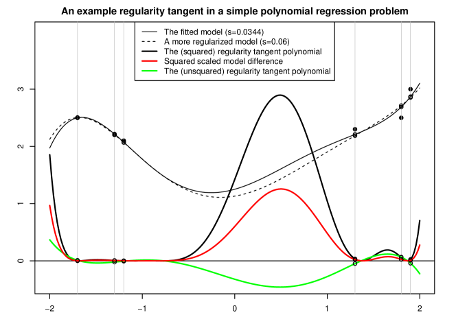
Figure 1:

The responses are calculated as

$$y(x)=F(x;\theta)=\mathop{\mathrm{power}}(x)^{\top}\theta$$ (72)

where $\mathop{\mathrm{power}}(x)=(1,x,\cdots,x^{5})$ is a 6-element vector containing powers of $x$ (or a 6-column matrix, if $x$ is a vector, with each row corresponding to one data point). If $x$ is a vector of unlabeled data points, and $y$ contains the labels, the optimal $\theta$ may be calculated as

$$\theta=(X^{\top}X+sI)^{-1}X^{\top}y$$ (73)

where $X=\mathop{\mathrm{power}}(x)$. We use the convention that $y$ and $\theta$ are column vectors. This is the regularized version of the well-known formula for the parameters of a linear regression problem, called the normal equations, which incidentally takes the familiar form of an inverse-Hessian-vector product, where $X^{\top}y$ is the gradient at $\theta=0$ and $X^{\top}X+sI$ is the Hessian. The (regularized) normal equations derived by setting the gradient of the (regularized) objective function to zero:

$$0 =\frac{\mathrm{d}}{\mathrm{d}\theta}\left(\sum_{i}(X_{i}\theta-y_{i})^{2}+s\theta^{\top}\theta\right)$$ (74)

$$=\sum_{i}2X_{i}(X_{i}\theta-y_{i})+2s\theta$$ (75)

$$0 =-X^{\top}y+X^{\top}(X\theta)+s\theta$$ (76)

$$X^{\top}y =(X^{\top}X+sI)\theta$$ (77)

$$\theta =(X^{\top}X+sI)^{-1}X^{\top}y$$ (78)

where $X_{i}$ denotes row $i$ of $X$. It is equivalent to Newton’s method in this model, which converges after a single iteration because the objective function is quadratic.

The regularity tangent is calculated as

$${\partial\theta^{*}\over\partial s} =-H^{-1}\rho=-(X^{\top}X+sI)^{-1}(2\theta)$$ (79)

Figure 2 illustrates how the optimal regularity was calculated by minimizing the model’s generalization error, which is estimated using leave-one-out cross-validation (LOOCV). It is apparent that local minima can exist, although in this example the fact is more pronounced due to the small number of data points. It is also easy to produce examples where the optimal regularity is outside of the range of values we show in this plot, in other words it converges to zero or infinity.

Figure 2:

Figure 3 compares the RT-based ($\mathcal{I}_{\textrm{up,reg}}=\frac{\mathrm{d}R}{\mathrm{d}\varepsilon}=\frac{\mathrm{d}L}{\mathrm{d}s}$) SLD query heuristic with the squared-influence heuristic derived from the traditional $\mathcal{I}_{\textrm{up,loss}}$ ($=\frac{\mathrm{d}L}{\mathrm{d}\varepsilon}$) influence function.

The query heuristic curves are normalized to have the same RMS values, so multiplication by a constant has no effect. In this model the loss gradient contains a factor proportional to the residual $X\theta-y$ and we simply omit this factor when calculating the “unlabeled” version of the query heuristic, i.e. when we don’t know $y$. Rather than comparing the influence between $z$ and $z^{\prime}$

$$\mathcal{I}_{\textrm{up,loss}}(z,z^{\prime})=-\sigma_{z^{\prime}}^{\top}H\sigma_{z}$$ (80)

we are using an unlabeled version

$$\mathcal{I}_{\overline{\textrm{up}}\textrm{,loss}}(x,z^{\prime})=-\sigma_{z^{\prime}}^{\top}H\bar{\sigma}_{x}$$ (81)

where $\bar{\sigma}_{x}=2\mathop{\mathrm{power}}(x)$, which is within a factor of the “doubly-unlabeled” influence function

$$\mathcal{I}_{\overline{\overline{\textrm{up}}}\textrm{,loss}}(x,x^{\prime})=-\bar{\sigma}_{x^{\prime}}^{\top}H\bar{\sigma}_{x}$$ (82)

and thus equivalent when used in the SI (squared influence) query heuristic.

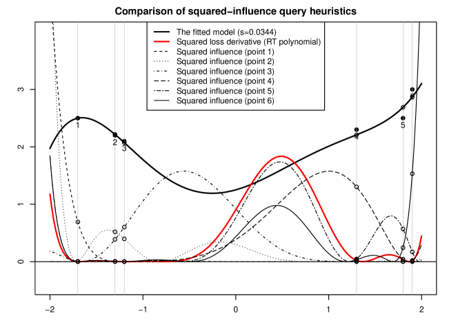
Figure 3:

The factor becomes relevant when we are summing influence functions, as the labeled SSI $Q(x)=\sum_{z}\mathcal{I}_{\overline{\textrm{up}}\textrm{,loss}}(x,z)^{2}$ and STI $Q(x)=\left(\sum_{z}\mathcal{I}_{\overline{\textrm{up}}\textrm{,loss}}(x,z)\right)^{2}$ give lower weight to data points with small residuals, while the unlabeled SSI $Q(x)=\sum_{x^{\prime}}\mathcal{I}_{\overline{\overline{\textrm{up}}}\textrm{,loss}}(x,x^{\prime})^{2}$ and STI $\left(\sum_{x^{\prime}}\mathcal{I}_{\overline{\overline{\textrm{up}}}\textrm{,loss}}(x,x^{\prime})\right)^{2}$ do not depend on $y$ and so give “equal” weight to each point within the semantics of the model, which is to say that the points are weighted independently of their residuals. For this reason the multi-point influence based query heuristics SSI (green) and STI (blue) come in labeled and unlabeled versions.

The unlabeled versions appear more “equitable”, covering a smaller range of values and being slightly bounded away from zero. The labeled versions are dominated by the influence of point 5, which has the highest residual. The red curve showing the squared loss derivative actually overlaps the blue curve “square total influence (labeled)”, but is shown scaled slightly higher so both curves can be seen on the plot.

That the curves are the same can be explained as follows. The fact that, in a trained model, the gradient of the model objective with respect to $\theta$ must be zero implies that a gradient of the regularizer is equal to the negative of the sum of the loss gradients. So, when the (labeled) influence functions for each data point are added together, we obtain the negative regularity tangent. Thus, differentiating by the regularity to calculate the regularity tangent, as we have proposed in this paper, can be seen as an efficient way of calculating the “total influence” of a dataset.

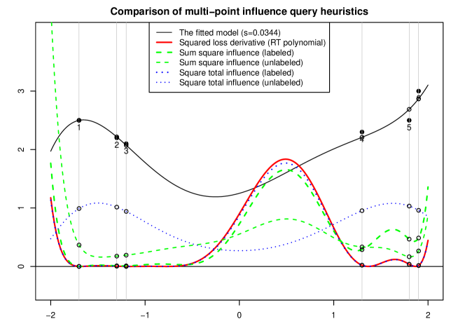
Figure 4:

We hope that these plots have been helpful in visualizing the quantities under discussion in this paper. They were generated using R.

Obviously, future versions of this section should contain a comparison of the various query heuristics under consideration, which at least evaluates their suitability for active learning in the simple polynomial regression model that we have been using here.

This is not expected to be difficult, but time constraints force us to postpone such experiments for later. There is also the question of testing the methodology in a more “real world model” setting, which is where we hope it will be useful. This must also be regrettably postponed, but the number of query heuristics that are theoretically efficient enough for use in very large models seems sufficiently constrained that one might hope the optimal heuristic to be among those we have proposed in section 3.2.

3.4 Regularity in a multi-user setting

This section describes the hierarchical use of regularization in a setting where individual users are attempting to train models that exchange information by inheriting from a shared template model containing all of the user interactions. This setting is important because multiple users deserve multiple models, and therefore multiple different regularities; and yet it may be desirable to combine information learned from each user so that interactions are not wasted. Particularly when a user is new to the system, we would like the first few interaction cycles to benefit from knowledge that had been gained from other users, so that training the model doesn’t have to restart from scratch each time.

A simple version of this idea might use the same regularization coefficient for each user, but to use a regularizer that penalizes the deviation of $\theta$ from some global parameter vector $\theta_{0}$, rather than (as in the usual case) its deviation from zero:

$$R(s,\theta)=s\lVert\theta-\theta_{0}\rVert_{1}$$ (83)

We suggest $\mathcal{L}_{1}$ regularization here because it enforces sparsity in the deviation $\theta-\theta_{0}$, so that each user’s $\theta$ differs from the base model $\theta_{0}$ at only a finite number of indices. Although $\mathcal{L}_{2}$ regularization is slightly simpler to implement because the regularizer is smooth, $\mathcal{L}_{1}$ regularization could be useful in the case of very large models, where storage considerations prevent us from being able to make a full copy of the parameter vector for each user. The shared parameter vector $\theta_{0}$ is optimized using data from as many users as possible, perhaps using the same regularity hyperparameter, and it will have its own regularity tangent $\dot{\theta}_{0}$. The regularity tangent $\dot{\theta}$ for a single user will inherit from the common $\dot{\theta}_{0}$:

$$\dot{\theta}=\frac{\mathrm{d}\theta}{\mathrm{d}s}={\partial\theta\over\partial\theta_{0}}\frac{\mathrm{d}\theta_{0}}{\mathrm{d}s}+\left(\frac{\mathrm{d}\theta}{\mathrm{d}s}\right)_{(\theta_{0})}$$ (84)

where $\left(\frac{\mathrm{d}\theta}{\mathrm{d}s}\right)_{(\theta_{0})}$ means taking the derivative of $\theta$ with respect to $s$ while considering $\theta_{0}$ to be constant. This fact ensures that each user’s model has a non-zero regularity tangent even before any data points have been seen, which is important because it means that the first query shown to a user is based on the curiosity expressed by the common model, and need not be random. It is not necessary to calculate the full Jacobian matrix ${\partial\theta\over\partial\theta_{0}}$, as our usual method for calulating $\dot{\theta}$ using (forward-mode) automatic differentiation should yield it more directly.

The idea could be extended to use some kind of dimensionality reduction on $\theta_{0}$ so that each user’s deviation from it is described by a very small number of parameters, representing a “personality type” for example, which are learned over the course of interacting with him. (An $\mathcal{L}_{2}$ regularizer would of course be suitable for this.)

Returning to the $\lVert\theta-\theta_{0}\rVert_{1}$ model, we note that for very large models the calculation of $\dot{\theta}_{0}$ should proceed in a very different way from the calculation of $\dot{\theta}$. While $\dot{\theta}_{0}$ would be calculated stochastically using SGDF (which we introduce in section 3.5) and batches of data points, the interaction history of a single user would usually fit into a single batch and so $\dot{\theta}$ could be calculated using more efficient second-order methods like NLCG (see section 3.8), which require a non-stochastic objective, presuming that these could be adapted to work well with $\mathcal{L}_{1}$ regularization. It seems that this or a similar hybrid optimization approach might be the best way to give large language models a sense of curiosity about their data, in addition to providing them with the ability to adapt to information coming from an individual user, without necessarily increasing the complexity of inference in the model.

We next explore the case where a multi-user model incorporates a different regularizer for each user. This is less interesting from the perspective of modeling, but attempts to explore a natural generalization to the regularization concept and look at how it interacts with the idea of regularity tangents and query heuristics. Consider a model which contains certain user-specific parameters $\theta_{M_{i}}$ (indexed by elements of the set $M_{i}$) for some set of users indexed by $i$. We might find it interesting to use per-user regularization coefficients $c_{i}$ whose distributions are controlled by a single regularity hyperparameter $s$:

$$R(s,(c,\theta,\alpha))=s\sum_{i}c_{i}^{2}+\sum_{i}\left(\alpha c_{i}\lVert\theta_{M_{i}}\rVert^{2}-{\left|M_{i}\right|\over 2}\log\alpha c_{i}\right)$$ (85)

In the Bayesian interpretation, the second term is saying that the parameters for user $i$, namely $\theta_{M_{i}}$, are given a prior consisting of independent normal distributions with variance ${1\over 2\alpha c_{i}}$ and mean 0; see the discussion below equation 11. We multiplied the precision $c_{i}$ by $\alpha$ which is to say half the Bayesian precision $2\alpha$ of the response variables, following equation 15. We also gave the $c_{i}$ variables normal distributions with mean 0 via the initial term. The ${\left|M_{i}\right|\over 2}\log\alpha c_{i}$ term is contributed from the normalization constant of $P(\theta_{M_{i}}|c_{i})$, which cannot be ignored because it depends on $c_{i}$ which (unlike $s$) is a new model parameter in $\theta$. This “regularizer” might be used with a system that has data coming from different users and wants to employ a slightly different prior when optimizing over each user’s parameter space, thus preferring simpler models for some users than others. The prior distribution over the “sub-regularities” $c_{i}$ is controlled by $s$, so that there is still only one regularity hyperparameter ($s$) to be optimized outside of the normal (gradient descent) training of $\theta$.

In equation 85 we should properly consider the coefficients $c_{i}$ as elements of the vector $\theta$, with say $\theta_{\hat{c}_{i}}\equiv c_{i}$ for each user $i$, where $\theta_{\hat{c}_{i}}$ denotes the index of $\theta$ being used to hold $c_{i}$. Then $\rho$ will only depend on $\theta_{\hat{c}}\equiv\{c_{i}|i\}$:

$$\rho\equiv{\partial^{2}f\over\partial\theta\partial s}\textrm{ ,\quad}\rho_{j}=\left\{\begin{array}[]{lcl}2c_{i}&:&j=\hat{c}_{i}\\ 0&:&\textrm{otherwise}\\ \end{array}\right.$$ (88)

Even though $(\sigma_{z})_{i}$ may be zero except at the indices of certain per-user parameters $i\in M_{j}$, where $z$ is a data point coming from user $j$, and $\rho_{i}$ may be non-zero only at indices $\hat{c}_{j}$ not intersecting any of the $M_{j}$, the regularity adjoint $\frac{\mathrm{d}L(z,\theta^{*})}{\mathrm{d}s}=\frac{\mathrm{d}\theta^{*}}{\mathrm{d}s}^{\top}\sigma_{z}=-\rho^{\top}H^{-1}\sigma_{z}$ which combines these two vectors may still in general be non-zero. That is due to couplings which will exist in the inverse Hessian matrix $H^{-1}$ between the non-overlapping sets of parameter indices. Thus although in this model our $\mathcal{I}_{\textrm{up,reg}}(z)=-\rho^{\top}H^{-1}\sigma_{z}$ is computing $\frac{\mathrm{d}\lVert c\rVert^{2}}{\mathrm{d}\varepsilon}$, this quantity itself depends indirectly on the per-user parameter change $\frac{\mathrm{d}\lVert\theta_{M_{i}}\rVert^{2}}{\mathrm{d}\varepsilon}$ through $c_{i}$, where $i$ is the user corresponding to data point $z$. Because $L(z,\theta)$ is only connected to $s$ through $c_{i}$, we can write $\theta^{*}(s)=\theta^{*}(c_{i}^{*}(s))$ and

$$\frac{\mathrm{d}\lVert c\rVert^{2}}{\mathrm{d}\varepsilon}=\frac{\mathrm{d}L}{\mathrm{d}s} =\sum_{j}\frac{\mathrm{d}L}{\mathrm{d}c_{j}}\frac{\mathrm{d}c_{j}}{\mathrm{d}s}$$ (89)

This is assuming there is no overlap between the per-user parameter vector indices.

$$\frac{\mathrm{d}L}{\mathrm{d}s}=\frac{\mathrm{d}L}{\mathrm{d}c_{i}}\frac{\mathrm{d}c_{i}}{\mathrm{d}s} =\frac{\mathrm{d}\left(2sc_{i}+\alpha\lVert\theta_{M_{i}}\rVert^{2}-{\left|M_{i}\right|\over 2c_{i}}\right)}{\mathrm{d}\varepsilon}\frac{\mathrm{d}c_{i}}{\mathrm{d}s}$$ (90)

the long quantity being differentiated on the right-hand side being ${\partial R\over\partial c_{i}}$ because

$$\frac{\mathrm{d}L}{\mathrm{d}c_{i}}=\frac{\mathrm{d}}{\mathrm{d}c_{i}}{\partial f\over\partial\varepsilon}=\frac{\mathrm{d}}{\mathrm{d}\varepsilon}{\partial f\over\partial c_{i}}=\frac{\mathrm{d}}{\mathrm{d}\varepsilon}{\partial R\over\partial c_{i}}$$ (91)

Thus for up-weighting a data point belonging to user $i$, which is expected to only affect parameters in $\theta_{M_{i}}$, we have that the regularity adjoint of the loss $\frac{\mathrm{d}L}{\mathrm{d}s}(z,\theta)$ is measuring the effect on $\lVert c\rVert^{2}$, equivalently $c_{i}^{2}$, of up-weighting point $z$. But this is also approximately equal to the $\varepsilon$ adjoint of a measure of the complexity of the parameters $\theta_{M_{i}}$ specific to user $i$: $\alpha\lVert\theta_{M_{i}}\rVert^{2}$. (Here we have omitted the $2sc_{i}$ and $-{\left|M_{i}\right|\over 2c_{i}}$ terms that were in the numerator of (90), because these are constant with respect to $\varepsilon$.)

This quantity is scaled by a user-specific constant $\frac{\mathrm{d}c_{i}}{\mathrm{d}s}$ in (90) which is part of $\frac{\mathrm{d}\theta}{\mathrm{d}s}$, measuring something like our degree of interest in user $i$. This scale factor does not affect the query heuristic, and can be left in, as it is the same for every data point belonging to a given user.

The above model can be represented by the probabilistic program, where $N$ is the normal distribution:

$$c_{i} \leftarrow N(0,{1\over 2s})$$ (92)

$$\theta_{M_{i}} \leftarrow N(0,{1\over 2\alpha c_{i}})$$ (93)

$$y_{j} \leftarrow N(\theta_{M_{i}}^{\top}x_{i},{1\over 2\alpha})$$ (94)

In (92) above, the regularity $s$ could equivalently be replaced with $\alpha s$, to make it look like (16), but we could not then simply factor $\alpha$ out of the resulting negative log likelihood objective because of the normalization constants which depend on it nonlinearly.

The same idea could be extended to give each user $i$ a more complicated prior over his parameters $\theta_{M_{i}}$, for example with a system-wide mean $\theta_{0}$ and one or more principal dimensions of variation, with $\theta_{M_{i}}^{*}(s)$ reacting to changes in $s$ through these intermediate variables. As a start, we could consider for example generating a linear regression model from the following probabilistic program:

(Gamma parameters, $$\theta \leftarrow N(0,{1\over 2\alpha s})$$) (95)

$$\kappa \leftarrow\textrm{Gamma}(\ldots)$$ (96)

$$\theta^{(j)} \leftarrow N(\theta,{1\over 2\alpha\kappa})$$ (97)

$$c_{j} \leftarrow\textrm{Gamma}(\ldots)$$ (98)

$$y_{i} \leftarrow N(\theta^{(o_{i})\top}x_{i},{1\over 2\alpha c_{o_{i}}})$$ (99)

This model gives each user $j$ a separate parameter vector $\theta^{(j)}$ taken to be near some prototype $\theta^{(0)}$, with precision controlled by $\kappa$, and furthermore assumes that each user’s data points are generated with a different precision, controlled by $c_{j}$. The index $o_{i}$ refers to the user (“owner”) for data point $z_{i}$. The Gamma prior over $\kappa$ and $c_{j}$ is the conjugate prior for the precision of a normal distribution, and therefore can be adjusted to capture the effect of simulated observations.

In creating a regression problem for this model, the last “sampling operation” $y_{i}\leftarrow N(\ldots)$ gives rise to a sum of weighted losses, with each loss term having weight $\alpha c_{j}$ for points belonging to user $j$, which is in contrast to the previous setting where each loss term had equal weight. The four earlier sampling operations comprise the regularizer, which has multiple terms for each user. Each loss also contains a term $-{1\over 2}\log\alpha c_{i}$, which captures $\log Z$ in the last distribution. Here only $x$ and $y$ are observed variables; $\alpha$ is an arbitrary positive number and a scale hyperparameter that does not enter into the model complexity. There are a variety of ways to choose $\alpha$, which may for example be optimized as a hyperparameter like $s$, or treated as a model variable with a Normal or Gamma prior, or estimated directly from the data. The optimal value of $\alpha$ is a measure of the variance of the true response variable $y$ with respect to the model’s predictions $\theta^{\top}x$. And $s$ is the regularity hyperparameter. The rest of the variables are model parameters to be optimized during (stochastic) gradient descent (remembering to at least occasionally take into account the gradient of the regularizer term, for example at the end of each pass through the data). The hyperparameter $s$ should perhaps be optimized to minimize a sum of the loss terms on a test data set, according to whatever performance metric is desired of the model, including for example reducing the weight of data points from users with low $c_{i}$, parroting the loss term coefficients appearing in the new empirical risk.

In summary, all of these regression problems seem amenable to the use of regularity tangents, introduced in the previous section, because regularity tangents have the ability to link various interdependent model parameters to each other through the regularizer term. From these brief algebraic investigations we would like to infer that our method might be successfully applied to models with hierarchical notions (meaning layered or structured) of model complexity, including but not limited to those introduced in this section, rather than just to the uniform regularizer model of section 2.1 (e.g. (4)).

3.5 Computing influence functions

We have been talking about influence functions and other quantities which, according to the implicit function theorem, are constructed by multiplying the negative inverse Hessian matrix with one or more gradient vectors. We have so far set aside the question of calculating the Hessian $H$ or inverse Hessian $H^{-1}$. Although we have been motivated by efficiency concerns to propose approximations based on differential calculus to estimate the effects of adding or removing a data point from the corpus, so as to avoid the need for retraining the model after each addition or subtraction, these approximations have resulted in formulae involving the Hessian which can itself be intractable to compute. If the number of parameters $p$ is very large then the Hessian, which has $p^{2}$ entries, may even be impossible to store in memory, let alone invert. This is the case for many commonly-used models in machine learning. Some modern models are so large that even the parameter updates of Stochastic Gradient Descent would be prohibitively expensive but for the fact that the gradient vectors ${\partial L\over\partial\theta}$ are designed to be sparse through the use of normally-zero activation functions like the “ramp function” $\max(x,0)$ in the network that defines the model. However, we can show that it is possible to calculate influence functions efficiently even in the case of such very large models, with the same time complexity as training the model.

To explain this, some familiarity with automatic differentiation is useful. Automatic differentiation is a family of methods based on the chain rule of calculus for computing the derivatives of programs. These methods generally fall into two classes: reverse-mode automatic differentiation, also knows as back-propagation; and forward-mode automatic differentiation, which may be implemented using “dual numbers”. Reverse-mode automatic differentiation computes the derivative of a single output variable with respect to multiple input variables, while forward-mode automatic differentiation computes the derivative of multiple output variables with respect to a single input variable. Both methods have a runtime proportional to the runtime of the original program (implying that they all have the same time complexities), although (unlike forward-mode, which doesn’t change the memory complexity), reverse-mode automatic differentiation also requires an additional amount of memory proportional to the runtime. A key observation is that automatic differentiation can be applied to any program, even one which is iterative. [3, 19, 5, 6]

Reverse-mode automatic differentiation is typically used to calculate the gradients ${\partial f\over\partial\theta}$ in gradient descent and ${\partial L(z)\over\partial\theta}$ in stochastic gradient descent (SGD). We can additionally apply forward-mode automatic differentiation to gradient descent to obtain, together with the optimal parameter vector $\theta^{*}$, an estimate $\frac{\mathrm{d}\theta^{*}}{\mathrm{d}s}$ which is the regularity adjoint with respect to $\theta^{*}$.

Writing $\dot{\theta}$ for $\frac{\mathrm{d}\theta}{\mathrm{d}s}$, we simply substitute the “dual number” $\theta+\dot{\theta}\mathrm{d}s$ in the gradient descent algorithm, which becomes

$$\theta_{t+1}+\dot{\theta}_{t+1}\mathrm{d}s\leftarrow(\theta_{t}+\dot{\theta}_{t}\mathrm{d}s)-\eta_{t} \left({\partial\over\partial\theta}f(\theta_{t}+\dot{\theta}_{t}\mathrm{d}s)=\right.$$ (100)

$$\left.{\partial\over\partial\theta}f(\theta_{t})+\left({\partial^{2}\over\partial\theta\partial s}f(\theta_{t})+{\partial^{2}\over{\partial\theta}^{2}}f(\theta_{t})\cdot\dot{\theta}_{t}\right)\mathrm{d}s\right)$$ (101)

So the update of the dual part ($\mathrm{d}s$ terms) becomes

$$\dot{\theta}_{t+1}\leftarrow\dot{\theta}_{t}-\eta_{t}(\rho+H\dot{\theta}_{t})$$ (102)

where the complexity gradient $\rho={\partial^{2}f\over\partial\theta\partial s}={\partial\over\partial\theta}R_{s}(\theta_{t})$ was defined in equation 59, and the Hessian H is evaluated at $\theta_{t}$. Note that this is a hybrid application of both forward-mode automatic differentiation ($\frac{\mathrm{d}}{\mathrm{d}s}$) and reverse-mode automatic differentiation (${\partial\over\partial\theta})$. The expanded second term contains a so-called “Hessian vector product”, which quantity can be easily calculated through the use of dual numbers in the gradient expression ${\partial\over\partial\theta}f(\theta_{t}+\dot{\theta}_{t}\mathrm{d}s)$. In fact it is well known that Hessian-vector products may be calculated as easily as the gradient of a function [20]. This may be done using either forward-mode or reverse-mode automatic differentiation, or numerical approximation, and methods for computing a Hessian-vector product are available in popular automatic-differentiation libraries. For example, using forward-mode automatic differentiation ($\frac{\mathrm{d}}{\mathrm{d}\varepsilon}$) after the reverse-mode (${\partial\over\partial\theta})$,

$$\left.\frac{\mathrm{d}}{\mathrm{d}\varepsilon}\right|_{\varepsilon=0}{\partial\over\partial\theta}f(\theta+\varepsilon v)={\partial^{2}\over{\partial\theta}^{2}}f(\theta)\cdot v=Hv$$ (103)

where $H$ is the Hessian ${\partial^{2}f\over{\partial\theta}^{2}}$. Or using reverse-mode automatic differentiation (twice):

$${\partial\over\partial\theta}\left(v^{\top}{\partial f\over\partial\theta}\right)=v^{\top}{\partial^{2}f\over{\partial\theta}^{2}}=v^{\top}H$$ (104)

which seems to be the method used by the popular PyTorch library. The competing JAX library seems to be able to compute a Hessian-vector product using both methods.

It is possible to produce a similarly instrumented version of gradient descent using only reverse-mode automatic differentiation via equation 104 (see [1]), but the hybrid forward-reverse algorithm of equation 100 seems simpler and faster if forward-mode is available.

We have noticed in some simple experiments that (102) can be used as-is to calculate $\dot{\theta}$ alongside algorithms like Adam where $\eta$ depends on the history of gradient vectors.

In the above algorithm, the parameter derivatives $\dot{\theta}$ may be initialized to random numbers, or they may be primed with a previously converged value, just as with the parameter vector $\theta$. For well-conditioned problems, the final value of $\dot{\theta}$ should be insensitive to the initial conditions. If it converges, from (102) we can see that it should do so to a vector $\dot{\theta}$ with $H\dot{\theta}=-\rho$. It is of course possible to run the non-dual version of gradient descent to convergence, and then use the resulting $\theta^{*}$ as a starting point of the dual number algorithm, which will theoretically leave $\theta$ stationary and only update the derivatives $\dot{\theta}$ at each iteration.

Instead of computing the gradient of the whole objective function $f$ during each update of gradient descent, we could cycle through the available labeled data points $z$ and use the loss gradient ${\partial L\over\partial\theta}(z)$ as a “randomly sampled” proxy for ${\partial f\over\partial\theta}$. This is the idea behind the popular “stochastic gradient descent” (SGD) algorithm, defined in equation 27. As with gradient descent above, SGD can also be applied to dual numbers, to yield an algorithm that estimates $\frac{\mathrm{d}\theta^{*}}{\mathrm{d}s}$ along with $\theta^{*}$. With this modification the SGD parameter updates become (compare to equations 26, 101 and 27):

$$\theta_{t+1}+\dot{\theta}_{t+1}\mathrm{d}s\leftarrow(\theta_{t}+\dot{\theta}_{t}\mathrm{d}s)-\eta_{t} \left({\partial L\over\partial\theta}(z_{u_{t}},\theta_{t}+\dot{\theta}_{t}\mathrm{d}s)=\right.$$ (105)

$$\left.{\partial\over\partial\theta}L(z_{u_{t}},\theta_{t})+{\partial^{2}\over{\partial\theta}^{2}}L(z_{u_{t}},\theta_{t})\cdot\dot{\theta}_{t}\mathrm{d}s\right)$$ (106)

where the expanded form on the second line is missing the ${\partial^{2}\over\partial\theta\partial s}$ term from 101 as $L$ does not depend on $s$. We call this algorithm “stochastic gradient descent with forward-mode differentiation” or SGDF. The update of the regularity tangent can also be written separately from that of the parameters:

$$\theta_{t+1} \leftarrow\theta_{t}-\eta_{t}{\partial\over\partial\theta}L(z_{u_{t}},\theta_{t})$$ (107)

$$\dot{\theta}_{t+1} \leftarrow\dot{\theta}_{t}-\eta_{t}{\partial^{2}\over{\partial\theta}^{2}}L(z_{u_{t}},\theta_{t})\cdot\dot{\theta}_{t}$$ (108)

We again assume that the regularization term in the definition of the objective $f$ is taken into account intermittently, for example at the end of each batch (equation 29). For that update we have

$$\theta_{t+1}+\dot{\theta}_{t+1}\mathrm{d}s\leftarrow(\theta_{t}+\dot{\theta}_{t}\mathrm{d}s)-\eta_{t}\left({\partial\over\partial\theta}R(s,\theta_{t})+\left({\partial^{2}\over\partial\theta\partial s}R(s,\theta_{t})+{\partial^{2}\over{\partial\theta}^{2}}R(s,\theta_{t})\cdot\dot{\theta}_{t}\right)\mathrm{d}s\right)$$

or equivalently

$$\theta_{t+1} \leftarrow\theta_{t}-\eta_{t}{\partial\over\partial\theta}R(s,\theta_{t})$$ (109)

$$\dot{\theta}_{t+1} \leftarrow\dot{\theta}_{t}-\eta_{t}\left({\partial^{2}\over\partial\theta\partial s}R(s,\theta_{t})+{\partial^{2}\over{\partial\theta}^{2}}R(s,\theta_{t})\cdot\dot{\theta}_{t}\right)$$ (110)

which in the case of $R(s,t)=s\lVert\theta\rVert^{2}$ becomes

$$\theta_{t+1}+\dot{\theta}_{t+1}\mathrm{d}s\leftarrow(\theta_{t}+\dot{\theta}_{t}\mathrm{d}s)-\eta_{t}\left(2s\theta_{t}+\left(2\theta_{t}+2s\dot{\theta}_{t}\right)\mathrm{d}s\right)$$ (111)

or equivalently

$$\theta_{t+1}\leftarrow\theta_{t}-\eta_{t}(2s\theta_{t}) =(1-2\eta_{t}s)\theta_{t}$$ (112)

$$\dot{\theta}_{t+1}\leftarrow\dot{\theta}_{t}-\eta_{t}\left(2\theta_{t}+2s\dot{\theta}_{t}\right) =(1-2\eta_{t}s)\dot{\theta}_{t}-2\eta_{t}\theta_{t}$$ (113)

The $\theta_{t+1}$ update is rightly called “shrinkage” because it shrinks each component of $\theta$ by the factor $(1-2\eta s)$. The $\dot{\theta}_{t+1}$ update also shrinks $\dot{\theta}$ by $(1-2\eta s)$ but additionally subtracts a vector proportional to $\theta$.

3.6 Equivalence of SGDF and LiSSA

Our “SGDF” algorithm computes $\frac{\mathrm{d}\theta^{*}(s)}{\mathrm{d}s}$, which as we have seen can also be written as $\frac{\mathrm{d}\theta^{*}(s)}{\mathrm{d}s}=-\left({\partial^{2}f\over{\partial\theta}^{2}}\right)^{-1}{\partial^{2}f\over\partial s\partial\theta}=-H^{-1}v$ where $H={\partial^{2}f\over{\partial\theta}^{2}}$ is the Hessian of $f$ and $v={\partial^{2}f\over\partial s\partial\theta}$ is a gradient of the regularizer term. It is straightforward to combine the two SGDF updates defined above, in equations 106 and 110, so that the regularizer is taken into account with every update. We show that the resulting algorithm generalizes an existing algorithm called LiSSA proposed by Agarwal in 2017 [1]. The purpose of LiSSA is to compute inverse-Hessian vector products $H^{-1}v$ from an objective function $f$ that can be written as an average of loss functions calculated at different data points, i.e. $f(\theta)={1\over n}\sum_{i}L(z_{u_{i}},\theta)$. The LiSSA algorithm requires that we have the ability to compute Hessian-vector products for the Hessians of the loss function evaluated at random data points, which as we have said can be done easily using standard automatic differentiation libraries. The LiSSA algorithm is based on the observation that

$$vH^{-1} =v{I\over I-(I-H)}=v\sum_{k=0}^{\infty}(I-H)^{k}$$ (114)

$$=\left(\left((\ldots)(I-H)+v\right)(I-H)+v\right)(I-H)+v$$ (115)

where the expansion on the second line is an application of a well-known trick for computing polynomials without exponentiation.

If $h_{t}$ is our current approximation to $H^{-1}v$ then this gives the update

$$h_{t+1}=v+(I-H)h_{t}$$ (116)

Since $H$ is an average of loss Hessians at each data point, we can approximate it stochastically by substituting the loss Hessian at a random data point. If we do this at every update, we get Agarwal’s “LiSSA-sample” algorithm, which is usually called LiSSA:

$$h_{t+1}=v+(I-l_{t})h_{t}$$ (117)

where $l_{t}$ is defined as the loss Hessian ${\partial^{2}\over{\partial\theta}^{2}}L(z_{u_{t}},\theta^{*})$ where $u$ is the (possibly repeating) sequence of random data point indices used for each update. [2, 1]

We now show how to introduce a step size $\eta$ into the LiSSA update by scaling the objective function and the parameter vector. We then show that the LiSSA updates with step size are equivalent to an application of forward-mode automatic differentiation (dual numbers) to SGD, as given in equations 106 and 110, on an objective function with a specially chosen regularizer term.

Scaling $f$ in the LiSSA algorithm would not be expected to change the location of the optimum parameter vector $\theta^{*}$, but the Hessian $H$ would be scaled by the same factor as $f$. As a first attempt, we apply LiSSA to an objective $f$ which has been scaled by $\eta$. This yields the following version of the algorithm, where $v$ has also been scaled by $\eta$ to keep the product $h\approx H^{-1}v$ the same:

$$-h_{t+1} =-\eta v-(I-\eta l_{t})h_{t}$$ (118)

$$=-h_{t}-\eta(v-l_{t}h_{t})$$ (119)

We can apparently get to the same equation by scaling $\theta$ by $\sqrt{\eta}$, which yields $\theta^{\prime}=\sqrt{\eta}\theta$, and

$$H^{\prime}={\partial^{2}\over{\partial\theta^{\prime}}^{2}}f=\left({\partial\theta\over\partial\theta^{\prime}}\right)^{2}{\partial^{2}\over{\partial\theta}^{2}}f={1\over\eta}H$$ (120)

Then we must write $v^{\prime}={v\over\eta}$ in order to keep the product $H^{-1}v$ the same. The new ($\theta$-scaled) LiSSA update becomes:

$$-h^{\prime}_{t+1} =-\eta v^{\prime}-(I-\eta l^{\prime}_{t})h^{\prime}_{t}$$ (121)

$$=-h^{\prime}_{t}-\eta(v^{\prime}-l^{\prime}_{t}h^{\prime}_{t})$$ (122)

Both 119 and 122 are equivalent to a stochastic gradient descent update with forward-mode (SGDF, equation 106) on the dual parameter vector $\dot{\theta}$ with step size $\eta$, where $-h\approx-H^{-1}v=-\left({\partial^{2}f\over{\partial\theta}^{2}}\right)^{-1}{\partial^{2}\over\partial\theta\partial s}f(\theta^{*})$ corresponds to $\dot{\theta}$, and $v={\partial^{2}\over\partial\theta\partial s}f(\theta^{*})$ is a gradient of the regularizer term, what we have called the complexity gradient $\rho$; for $\mathcal{L}_{2}$ regularization it is $2\theta$. We can see that LiSSA must correspond to a form of stochastic gradient descent where the regularizer term is considered at each parameter update, rather than at the end of batches, since $v$ is included in each update of $h_{t}$. Since the regularizer’s contribution to $\dot{\theta}$ is non-sparse, i.e. it touches every index, obviously for sparse models it is better to perform this update only at suitably spaced intervals.

It is not clear whether the authors of the LiSSA algorithm understood that a step size parameter could be introduced implicitly by scaling the parameters or the objective function, or by comparison to SGDF, or that the result would correspond to a form of SGD using forward-mode automatic differentiation. To turn a problem framed for LiSSA, i.e. to compute $H^{-1}v$ for some $f$ and $v$, into a regularity adjoint calculation problem, it seems sufficient to take

$$f(\theta)={1\over n}\sum_{i}L(z_{i},\theta)+R(s,\theta)$$ (123)

where $R(s,\theta)$ is chosen so that its gradient ${\partial^{2}\over\partial s\partial\theta}R(s,\theta)$ is equal to $v$, e.g. $R(s,\theta)=s\theta^{\top}v$. It should be enough to set $s$ to zero and only consider its adjoints, or $s$ can be chosen to reduce overfitting, as we described in section 2.2. There are comments in the published literature about LiSSA requiring careful tuning or showing poor convergence when $H$ is badly conditioned (see [11] or section 4.2 of [2]), and it seems possible that one or more versions of the algorithm with a step-size parameter as given here would have better behavior, but we have not tested this hypothesis yet. There is not an obvious way to choose the step size for LiSSA, but if SGDF is optimizing the parameters $\theta$ at the same time, then the dual components $\dot{\theta}$ will be updated with the same step size as the parameters $\theta$, and so that design choice will already have been made.

3.7 SGDF and hyperparameter optimization

In section 2.4.1 we proposed using influence functions to approximate the LOOCV estimate of the regularized model’s generalization error on a set of data points. In this section we return to the model selection theme and explore some possible uses for regularity tangents outside of active learning.

We return to the discussion of regularity adjoints, exploring some possible alternative uses outside of active learning. As we have shown, our loss derivative $\frac{\mathrm{d}L(z,\theta^{*}(s))}{\mathrm{d}s}$ is an influence function in the up-weighting sense, because it is theoretically equal to $\mathcal{I}_{\textrm{up,reg}}$, or the change in regularizer $R(s,\theta)$ when up-weighting a point $z$’s loss by $\varepsilon$; or in other words $\frac{\mathrm{d}R_{s}(\theta^{*}(\varepsilon))}{\mathrm{d}\varepsilon}$. We now point out that our influence function can also be used to optimize the regularity hyperparameter $s$ during cross-validation. In fact this can be done simultaneously with SGD(F). Simply divide the data set into two groups, a training set and a test set. Pick a data point $z$ from the training set and use ${\partial L\over\partial\theta}(z,\theta)$ and the gradient of the regularizer to update the parameters $\theta$ (with the current step-size in SGD, keeping track of $\frac{\mathrm{d}\theta}{\mathrm{d}s}\equiv\dot{\theta}$). Then, pick a random data point $z$ from the test set and use the (scalar-valued) “gradient” $\frac{\mathrm{d}L}{\mathrm{d}s}(z,\theta)$, calculated as ${\partial L\over\partial\theta}\cdot\frac{\mathrm{d}\theta}{\mathrm{d}s}$, to similarly update the regularity $s$.

We might hope this algorithm to produce a converged parameter vector $\theta^{*}$ minimizing the loss on the training set over $\theta$, simultaneously with a converged regularity $s^{*}$ such that $\theta^{*}(s^{*})$ maximizes with respect to $s$ the loss on the test set when using parameters $\theta^{*}(s)$. This is the standard goal when using cross-validation to optimize a hyperparameter such as $s$, and it can be achieved using some of the techniques we have presented for calculating $\frac{\mathrm{d}L}{\mathrm{d}s}$ with only a constant slow-down to the SGD algorithm per update.

Furthermore, it should be possible to modify this algorithm by moving points back and forth between the test and training sets, as long as this rearrangement is done sufficiently infrequently that $\theta^{*}$ can converge to its new value when the training set changes, but not so infrequently that $s^{*}$ shows excessive variation when the test set changes. Presumably, meeting both criteria requires using widely separate step sizes to update $s$ and $\theta$. It might also make sense to do these updates in batches, for example following each training batch with a test batch. One might hope that the resulting algorithm would be something like $k$-fold cross-validation, averaging over multiple test/training splits of the data.

We have not yet tested this idea but it is interesting to think about a simple gradient update algorithm like SGD that is capable of performing the same regularity hyperparameter optimizations as a methodology based on cross-validation, but on a continuous basis during a uniform training phase, keeping only a single copy of the parameter vector and its regularity tangent in storage, along with all the data points. It is also possible that this modified algorithm would be inefficient due to the need to update $s$ sufficiently slowly.

In either case it seems interesting to ask if the existence of a continuous algorithm for jointly optimizing $\theta$ and $s$ could lead to any insights about the linear algebra behind what is happening in regularized cross-validated regression, whether in the original or the modified (with migration of points between training and test sets) algorithm, and what this could teach us about model regularity. It is tempting to recommend the use of influence functions in the modified algorithm for making compensatory adjustments to $\theta$ every time the training set changes, but each such estimate requires a separate run of LiSSA/SGDF, as the influence of a data point $z$ on $\theta$, which we called $\mathcal{I}_{\textrm{up,params}}$, cannot be straightforwardly computed from the regularity tangent. Note that the optimal value of $s$ may change slightly every time points are added or removed from the training data, resulting in a new $\theta^{*}$ and a new value for the complexity $R_{s}(\theta^{*})$, so active learning and online learning algorithms could theoretically benefit from a training methodology that optimizes $\theta$ and $s$ together.

Many implementations of SGD do not use a regularizer but rely on early stopping to prevent overfitting (as we mentioned in section 2.3), with the decision to stop training usually made by periodically evaluating the model on some test data set and looking for the moment when the loss starts to increase. In such settings it should be possible to set $s=0$ and use a dummy regularizer like $s\lVert\theta\rVert^{2}$ just for the purpose of running the SGDF algorithm for e.g. active learning selectors, as we hypothesize that the calculation of $\dot{\theta}$ will still be valid and the loss-derivative model-complexity influence-function identity $\frac{\mathrm{d}L(z,\theta^{*})}{\mathrm{d}s}=\frac{\mathrm{d}R_{s}(\theta^{*}(\varepsilon))}{\mathrm{d}\varepsilon}$ will still approximately hold even if $s$ is (sub-optimally) set to 0, because the identity only depends on the identification of an optimum for $\theta$ and not $s$.

Finally, we would like to promote the generality of our algorithm and the techniques presented here by making an appeal to the universality of the regularization concept in continuous models, which is based on the simple and fundamental philosophical argument that models may be ranked by complexity, so that a single scalar hyperparameter suffices to compensate for overfitting.

3.8 Second-order optimization methods

We have been concentrating on gradient descent and its derivatives because they are currently used to train the largest machine learning models. However, optimization methods that use second-order derivative information can be much more efficient, and are mostly applicable to systems where the training data is small enough to fit into one “batch”, so that one may forego stochastic optimization when training the model. Such situations may in fact be common in interactive settings, as the entire history of a single user’s interaction with an application, or at least the salient parts of it, is likely to be small enough to fit into one training batch on commodity CPU hardware. Where the Hessian is small enough to be inverted, Newton’s Method may be used for training the model. This includes the “Iteratively Reweighted Least Squares” (IRWLS) algorithm which applies to a class of regression problems called “Generalized Linear Models” (GLMs) and is equivalent to Newton’s Method. In this complexity domain, since we can invert $H$, we may of course compute the trained regularity tangent directly as $\dot{\theta}^{*}=-H^{-1}\rho$ (equation 59).

Even when the full Hessian may not be computed, Hessian-vector products are generally available, and are asymptotically no more expensive than evaluating the model objective. Thus, provided that all the data fits in a batch, the Nonlinear Conjugate Gradient (NLCG) algorithm [21], which uses Hessian-vector product to determine step size and direction, is always applicable.

Theoretically, the NLCG algorithm itself will produce a correct regularity tangent as a byproduct of the optimization if we apply it to dual numbers as we did in equation 100 for gradient descent. However, in this domain of medium complexity it is also possible to compute the regularity tangent (or any other influence function) using the Conjugate Gradients method (CG), the linear method upon which NLCG is based, which can be seen as computing $H^{-1}\rho$ using Hessian-vector products. This RT computation can be done after running the model parameter optimization to convergence using ordinary (not dual number) arithmetic.

The second option may be more convenient, in other words calculating $\dot{\theta}$ only as a special step at the end of training, and it avoids layering three different kinds of automatic differentiation. These three transforms are needed to automatically propagate dual numbers through NLCG (already a second-order algorithm) as the influence of the dual variable on the step size becomes important here. In preliminary experiments it was not possible to ignore that dependency and still get accurate regularity tangents, as it had been with Gradient Descent and Adam. Furthermore, we would expect CG on $\dot{\theta}$ to have faster convergence if we run it separately after the convergence of $\theta$, since the algorithm won’t be tracking a moving target when $\theta=\theta^{*}$ is already fixed. This is what we recommend for medium-sized, i.e. single-batch, models where a deterministic method like NLCG can be used but Newton’s Method is unavailable due to the intractability of computing or storing the Hessian in the larger parameter space.

Provided that second-order methods can be used effectively in $\mathcal{L}_{1}$-regularized models, in spite of discontinuities in the gradient function, which seems to be the subject of several papers, we again note the possibility (brought up in section 3.4) for a hybrid learning system that trains a large model using a large commodity corpus and (multi-batch) stochastic gradient descent with sparse loss gradients to obtain a global parameter vector $\theta_{0}$ which is then refined using sparse updates via a (for example) $\lVert\theta-\theta_{0}\rVert$ regularizer and a second-order method like NLCG in a sinlge-batch mode where the “batch” of data consists of the (relatively short) interaction history with a given user. Such a “dual-mode” system could conceivably provide a tractable way for a large language model (or other large model) to change its beliefs and express curiosity in response to interactions with an individual user, in other words without adding to the time complexity of its responses. The records of such interactions could then be collected and used to further refine the base model $\theta_{0}$.

It seems that a curated data acquisition methodology which makes user-tuned models available that express curiosity about the base model $\theta_{0}$ might lead to more efficient training of large AI models and more compact and efficient knowledge representations. Furthermore it would be possible to substitute an existing AI model for a human user, leveraging the existing model to create a more compact version of itself, which could then be further refined by human input, and so on. Given the reasoning power of existing AI language models, it is somewhat frightening to speculate about the possible experience of interacting with an intelligent computer system that is actually able to be interested in a user’s beliefs and to express curiosity about them and perhaps even uncover contradictions. Provided that it can be made to work, there is furthermore the possibility for such a system to be used in interrogations by authorities of all kinds, which could lead to various abuses. The authors are however hopeful that humanity would ultimately benefit from the systems embodied in these ideas because of their potential for use in teaching.

4 Conclusion

Our goal has been to explore ways in which a standard machine learning regression model can be made to express a notion of curiosity. We have done this through the framework of Active Learning, in which a model is made to select unlabeled data points whose (labeled) addition to its training data would be somehow beneficial to the accuracy of the model.

In exploring this problem, we have introduced a concept and a quantity called a “regularity tangent” (section 3.1), which can be used for data point selection in active learning (ibid.), as well as for optimization of the regularity hyperparameter in models with explicit regularization (section 3.7). We showed that the inner product of the regularity tangent with the loss gradient at a data point is equivalent to the “influence” of that data point on the model complexity as defined by the model’s regularizer (section 3.1). Then we outlined some potentially useful active learning query heuristics that incorporate the regularity tangent (section 3.2). We discussed multi-user models where the regularizer penalizes deviation from a shared “global” parameter vector, as well as the application of regularity tangents to multi-user models where there is a hierarchy of regularizers (section 3.4). We showed how to calculate the regularity tangent in large models using a new algorithm called “Stochastic gradient descent with forward-mode automatic differentiation”, or SGDF (section 3.5), which we showed to be equivalent to a generalization of an existing algorithm called LiSSA (section 3.6). We also outlined how to compute the regularity tangent in small and medium-sized models where other optimization methods than gradient descent are feasible, which use second order derivative information, such as Newton’s Method and NLCG (section 3.8).

5 Acknowledgments

The author would like to thank Clayton Otey, David Duvenaud, Zoubin Ghahramani, David Liu, and Dennis and Logan for assistance and helpful feedback during various stages of this paper; but especially to my doctoral supervisor Zoubin, who also supervised my master’s thesis and thereby nurtured an early interest in Active Learning and Bayesian Machine Learning.

References

- [1] Agarwal, Bullins, and Hazan. Second-Order Stochastic Optimization for Machine Learning in Linear Time, 2017.
- [2] Koh and Liang. Understanding Black-box Predictions via Influence Functions, 2017.
- [3] Gilbert. Automatic differentiation and iterative processes, 1992.
- [4] Bengio. Gradient-Based Optimization of Hyper-Parameters, 1999.
- [5] Maclaurin, Duvenaud, and Adams. Gradient-based Hyperparameter Optimization through Reversible Learning, 2015.
- [6] Franceschi, Donini, Frasconi, and Pontil. Forward and Reverse Gradient-Based Hyperparameter Optimization, 2017.
- [7] Franceschi, Frasconi, Grazzi, and Pontil. Bilevel Programming for Hyperparameter Optimization and Meta-Learning, 2018.
- [8] Lorraine, Vicol, and Duvenaud. Optimizing Millions of Hyperparameters by Implicit Differentiation, 2020.
- [9] Cook and Weisberg. Residuals and Influence in Regression, 1982.
- [10] Liu. Influence Selection for Active Learning, 2021.
- [11] Schioppa et al. Scaling Up Influence Functions, 2021.
- [12] Xia et al. Reliable Active Learning via Influence Functions, 2023.
- [13] Cai, Zhang, and Zhou. Maximizing Expected Model Change for Active Learning in Regression, 2013.
- [14] Giordano et al. A Swiss Army Infinitesimal Jackknife, 2019.
- [15] Settles. Active Learning Literature Survey, 2010.
- [16] Cohn, Atlas, and Ladner. Improving Generalization with Active Learning, 1994.
- [17] Kingma and Ba. Adam: A Method for Stochastic Optimization, 2015.
- [18] Bengio. Practical Recommendations for Gradient-Based Training of Deep Architectures, 2012.
- [19] Domke. Generic Methods for Optimization-Based Modeling, 2012.
- [20] Pearlmutter. Fast Exact Multiplication by the Hessian, 1993.
- [21] Shewchuk. An Introduction to the Conjugate Gradient Method Without the Agonizing Pain, 1994.