Fast-Decaying Polynomial Reproduction

Abstract

Polynomial reproduction plays a relevant role in deriving error estimates for various approximation schemes. Local reproduction in a quasi-uniform setting is a significant factor in the estimation of error and the assessment of stability but for some computationally relevant schemes, such as Rescaled Localized Radial Basis Functions (RL-RBF), it becomes a limitation. To facilitate the study of a greater variety of approximation methods in a unified and efficient manner, this work proposes a framework based on fast decaying polynomial reproduction: we do not restrict to compactly supported basis functions, but we allow the basis function decay to infinity as a function of the separation distance. Implementing fast decaying polynomial reproduction provides stable and convergent methods, that can be smooth when approximating by moving least squares otherwise, it is very efficient in the case of linear programming problems. All the results presented in this paper concerning the rate of convergence, the Lebesgue constant, the smoothness of the approximant, and the compactness of the support have been verified numerically, even in the multivariate setting.

1 Introduction

Polynomials are widely utilized in approximation theory due to their ease of definition, implementation, and immediate error analysis by resorting to Taylor expansion. Local polynomial reproduction is crucial in estimating errors for various approximation techniques (cf. e.g. [Sch97, Fly06]). In [Wen01], in the case of radial basis functions with compact support, a bound for the Lebesgue constants, which is uniform and independent of the space dimension, is provided. However, oversampling may still occur.
The insights of certain arguments in [DW20] enable us to reformulate the structure of polynomial reproduction in a general context. It is possible to contextualize the Rescaled Localised Radial Basis Function method (RL-RBF), introduced in [DFQ14], more effectively using the idea of fast decaying polynomial reproduction. The convergence of the RL-RBF interpolant has been analyzed in [DW20] leaving open a conjecture on the sum of the cardinal functions related to the RL-RBF approximant.

This paper aims to provide a new approach to polynomial reproduction based on the assumption that the basis functions are only decaying to infinity. To provide a comprehensive overview, we also cite the recent monograph [BJ22], which offers a detailed account of the latest quasi-interpolation techniques. We point out that the flexibility of the fast-decaying polynomial reproduction framework will also permit an alternative approach to these schemes. Quasi-interpolation techniques with functions having non-compact support have been meticulously reviewed providing a characterization of the approximation space for approximants of functions in the Sobolev space $W^{k}_{\infty}$ (cf. [LC92]). Under certain conditions (algebraic decay and possible divergence at $0^{+}$) our scheme can retrace the construction in [LC92].
In our work, the Gaussian kernel will play an important role, as its behavior at $\infty$ can be precisely controlled and idea that returns to the controlled approximation already explored by G. Strang in [Str70]. In [MS96] we find explicit error expansions for approximate approximations using Gaussian kernels. In particular with that approach, we could construct very accurate approximations, but generally, the approximations do not converge. Indeed they showed that to achieve convergence, the method’s parameters must depend on the distribution of data in the domain. This is the context within which our work will make improvements.
The paper is organized as follows. In section 2, after recalling some necessary definitions, we present the concept of local polynomial reproduction in a quasi-uniform setting and some useful results that will be employed in the successive discussion. In section 3, the motivation for the new fast-decaying polynomial reproduction technique and evidence of its convergence and stability are presented. In the following sections 4 and 5 we apply the fast-decaying polynomial reproduction in two instances: the moving least squares method and the approximation by linear programming. In section 6 we present and discuss some numerical experiments. The numerical tests have been conducted by comparing approximation methods under different conditions applied in univariate and multivariate settings. The performances of the methods, the moving least squares approach, and the approximation by linear optimization, are evaluated in terms of their stability and convergence. The analysis was concluded by examining the behavior of basis functions with algebraic decay, given that they diverge in zero and represent a degenerate case for our framework. In section 7, we conclude by summarizing our results and outlining some possible developments.

2 Notations and preliminaries

We start by defining local polynomial reproduction (cf. e.g. [Wen04, Definition 3.1]). Let $X=\{x_{1},\dots,x_{N}\}\subseteq\Omega\subseteq\mathbb{R}^{d}$ be a finite subset of distinct points their separation radius and fill distance are defined as follows

$$q_{X}\coloneqq\frac{1}{2}\min_{i\neq j}\|x_{i}-x_{j}\|_{2},\qquad h_{X,\Omega}\coloneqq\sup_{x\in\Omega}\min_{1\leq j\leq N}\|x-x_{j}\|_{2}.$$

Definition 1.

For every finite set $X=\{x_{1},\dots,x_{N}\}\subseteq\Omega$ we consider the family of functions $u_{j}=u_{j}^{X}:\Omega\rightarrow\mathbb{R}$ for $1\leq j\leq N$. They provide a local polynomial reproduction of degree $\ell$ on $\Omega$ if there exist constants $h_{0},C_{1},C_{2}\in\mathbb{R}_{>0}$ such that

1. $\displaystyle\sum_{j=1}^{N}p(x_{j})u_{j}=p$ for each $p\in\pi_{\ell}(\mathbb{R}^{d})$,

2. $\displaystyle\sum_{j=1}^{N}|u_{j}(x)|\leq C_{1}$ for all $x\in\Omega$,

3. $u_{j}(x)=0$ if $\|x-x_{j}\|_{2}>C_{2}h_{X,\Omega}$

are satisfied for all $X$ with $h_{X,\Omega}\leq h_{0}$.

Notice that $\pi_{\ell}(\mathbb{R}^{d})$ is the space of polynomials of degree at most $\ell$ in $\mathbb{R}^{d}$.

If $f:\Omega\rightarrow\mathbb{R}$ is a function we can build a stable quasi-interpolation process by

$$z_{f,X}=\sum_{j=1}^{N}f(x_{j})u_{j}.$$ (1)

It is important to observe that the second condition guarantees that the process is stable, that is the Lebesgue constant is bounded. Indeed,

$$\begin{split}\left|\sum_{j=1}^{N}f(x_{j})u_{j}(x)-\sum_{j=1}^{N}\widetilde{f}(x_{j})u_{j}(x)\right|&\leq\sum_{j=1}^{N}|f(x_{j})-\widetilde{f}(x_{j})||u_{j}(x)|\leq\\ &\leq\max_{1\leq j\leq N}|f(x_{j})-\widetilde{f}(x_{j})|\sum_{j=1}^{N}|u_{j}(x)|\leq\\ &\leq\max_{1\leq j\leq N}|f(x_{j})-\widetilde{f}(x_{j})|C_{1}.\end{split}$$

Instead, the first and third conditions concern local polynomial reproduction. In this setting the functions $\{u_{j}\}_{j=1,\dots,N}$ are arbitrary (their smoothness is not relevant for the stability and convergence). Although the fast-decaying polynomial reproduction framework is fairly general, it is useful to add regularity to the domain and the node distribution in order to produce concrete methods. To this aim, we need to introduce two definitions: the interior cone condition for the approximation domain and the quasi-uniform node distribution.

Definition 2.

A bounded Lipschitz domain $\Omega\subseteq\mathbb{R}^{d}$ satisfies an interior cone condition, if there exists an angle $\vartheta\in(0,\pi/2)$ and a radius $r>0$ such that for every $x\in\Omega$ a unit vector $\xi(x)$ exists so that the cone

$$C(x,\xi(x),\vartheta,r)\coloneqq\{x+\lambda y:y\in\mathbb{R}^{d},\,\|y\|_{2}=1,\,\langle y,\xi(x)\rangle\geq\cos(\vartheta),\,\lambda\in[0,r]\}$$

is entirely contained in $\Omega$.

Definition 3.

A nodes distribution $X=\{x_{1},\dots,x_{N}\}$ is quasi-uniform with respect to a constant $c_{qu}>0$, if

$$q_{X}\leq h_{X,\Omega}\leq c_{qu}q_{X}\,.$$

The requirement $q_{X}\leq h_{X,\Omega}$ instead of $cq_{X}\leq h_{X,\Omega}$ with $c<1$ is not restrictive if $\Omega$ satisfies an interior cone condition with radius $r>0$ and angle $\vartheta>0$. In fact, if $q_{X}\leq r$ then for each $x_{i}\in X$ we can find $y\in\Omega$ with $\|y-x_{i}\|_{2}=q_{X}$. Indeed, if $\|z\|_{2}=1$ and $\langle z,\xi(x)\rangle\geq\cos(\vartheta)$ then

$$\|\underbrace{x_{i}+\lambda z}_{y}-x_{i}\|_{2}=\lambda\in[0,r]\,.$$

For any other $x_{j}\in\Omega$

$$\|y-x_{j}\|_{2}\geq\|x_{j}-x_{i}\|_{2}-\|y-x_{i}\|_{2}\geq 2q_{X}-q_{X}=q_{X},$$

that gives $h_{X,\Omega}\geq q_{X}$.

The Definition 3 is useful when we consider a sequence of data sets that have the same constant $c_{qu}$ and the fill distance becomes smaller and smaller.
Being interested in a RL-RBF approximation, if the node distribution is quasi-uniform, we need to check how many nodes of $X$ fall near each point of $x\in\Omega$. To quantify them we need the scaling parameter $\delta$ of our approximation scheme is bounded (cf. [DW20])

$$\gamma c_{\gamma}h_{X,\Omega}\leq\delta\leq c_{\gamma}h_{X,\Omega},$$ (2)

with $\gamma\in]0,1[$ and $c_{\gamma}>1$. For quasi-uniformity of $X$, inequality (2) becomes

$$\gamma c_{\gamma}q_{X}\leq\delta\leq c_{\gamma}c_{qu}q_{X}.$$ (3)

Finally, the existence of methods that reproduce polynomials locally is claimed by the following theorem [Wen04, Theorem 3.14].

Theorem 1.

Suppose that $\Omega\subseteq\mathbb{R}^{d}$ is compact and satisfies an interior cone condition with angle $\vartheta\in]0,\pi/2[$ and radius $r>0$. Fix $m\in\mathbb{N}$. Then, there exists constants $h_{0},C_{1},C_{2}$ depending on $m,\vartheta,r$ such that for every $X=\{x_{1},\dots,x_{N}\}\subseteq\Omega$ with $h_{X,\Omega}\leq h_{0}$ and every $x\in\Omega$ we can find real numbers $\{\widetilde{u}_{j}(x)\}_{j=1,\dots,N}$ with

• $\displaystyle\sum_{j=1}^{N}p(x_{j})\widetilde{u}_{j}(x)=p(x)$ for each $p\in\pi_{m}(\mathbb{R}^{d})$,

• $\displaystyle\sum_{j=1}^{N}|\widetilde{u}_{j}(x)|\leq C_{1}$,

• $\widetilde{u}_{j}(x)=0$ if $\|x-x_{j}\|_{2}>C_{2}h_{X,\Omega}$.

In particular, from the proof of the previous Theorem, the values for the constants involved, when $\vartheta\leq\pi/5$, are:

$$C_{1}=2,\qquad C_{2}=\frac{16(1+\sin(\vartheta))^{2}m^{2}}{3\sin(\vartheta)^{2}},\qquad h_{0}=\frac{r}{C_{2}}.$$

3 Fast-decaying polynomial reproduction

Generalizing Definition 1 we want to relax the hypothesis of the compact support by preserving the same rate of convergence (cfr. [Wen04, Theorem 3.2]).

Definition 4.

Let $\varphi:\mathbb{R}_{\geq 0}\rightarrow\mathbb{R}$ be a decreasing function such that $\lim_{n\to+\infty}\frac{\varphi(n+1)}{\varphi(n)}$ exists and it is strictly smaller than $1$. For every finite set $X=\{x_{1},\dots,x_{N}\}\subseteq\Omega$ we consider the family of functions $u_{j}=u_{j}^{X}:\Omega\rightarrow\mathbb{R}$ for $1\leq j\leq N$. It provides fast-decaying polynomial reproduction of degree $\ell$ on $\Omega$ with respect to $\varphi$ if there exist constants $C,h_{0}\in\mathbb{R}_{>0}$ such that

1. $\sum_{j=1}^{N}p(x_{j})u_{j}=p$ for each $p\in\pi_{\ell}(\mathbb{R}^{d})$,

2. $|u_{j}(x)|\leq C\varphi\left(\frac{\|x-x_{j}\|_{2}}{q_{X}}\right)$ for all $x\in\Omega$ and $j=1,\dots,N$

are satisfied for all $X$ with $h_{X,\Omega}\leq h_{0}$.

In what follows, the problem we are facing is to construct a stable approximation based on a fast-decaying polynomial reproduction scheme, as described in eq. (1), to approximate any smooth function $f:\Omega^{*}\rightarrow\mathbb{R}$ which is ${\cal C}^{m+1}(\Omega^{*})$, $\Omega^{*}$ being the closure of the convex hull of $\Omega$ (see Theorem 3 below).

3.1 Stability

We recall that the interpolation method described in [DFQ14] fulfills the fast-decaying polynomial reproduction framework for quasi-uniform data sets up to a conjecture, as stated in [DW20, Theorem 2.3, Lemma 3.1].

The following result, which is a straightforward generalization of [DW20, Corollary 2.5], proves the stability of the fast-decaying polynomial reproduction approach and it will be useful to prove later on its convergence.

Theorem 2.

Suppose that $X=\{x_{1},\dots,x_{N}\}\subseteq\mathbb{R}^{d}$ is an arbitrary data set and $\{u_{1},\dots,u_{N}\}$ is given by a fast-decaying polynomial reproduction method with respect to $\varphi$. Then, for every $\ell\in\mathbb{N}$ there exists a constant $K=K(\ell,C,\varphi,d)$ such that

$$\sum_{j=1}^{N}\|x-x_{j}\|_{2}^{\ell}|u_{j}(x)|\leq Kq_{X}^{\ell}\quad\textrm{ for }x\in\Omega.$$ (4)

with

$$K=3^{d}C\sum_{n=0}^{+\infty}(n+1)^{d+\ell-1}\varphi(n).$$ (5)

Proof.

Fix $x\in\Omega$. We define a sequence of sets $\{E_{n}\}_{n\in\mathbb{N}}$ that covers $\mathbb{R}^{d}$ as

$$E_{n}=\{y\in\mathbb{R}^{d}:nq_{X}\leq\|y-x\|_{2}\leq(n+1)q_{X}\}.$$

We note that if $x_{j}\in E_{n}$ then

$$B(x_{j},q_{X})\subseteq\{y\in\mathbb{R}^{d}:(n-1)q_{X}\leq\|y-x\|_{2}\leq(n+2)q_{X}\}=E_{n-1}\cup E_{n}\cup E_{n+1}\,.$$

In fact, if $y\in B(x_{j},q_{X})$ then $nq_{X}-q_{X}\leq\|x_{j}-x\|_{2}-\|x_{j}-y\|_{2}\leq\|y-x\|_{2}\leq\|y-x_{j}\|_{2}+\|x_{j}-x\|\leq q_{X}+(n+1)q_{X}$. Since $\{B(x_{j},q_{X})\}_{j=1,\dots,N}$ are pairwise disjoint

$$\bigcup_{j:x_{j}\in E_{n}}B(x_{j},q_{X})\subseteq\overline{B(x,(n+2)q_{X})}\setminus B(x,(n-1)q_{X})$$

a volume comparison gives for $n\geq 1$

$$\#\{x_{j}:x_{j}\in E_{n}\}\leq(n+2)^{d}-(n-1)^{d}\leq 3^{d}n^{d-1}\leq 3^{d}(n+1)^{d-1},$$

that holds also for $n=0$ because $2^{d}\leq 3^{d}$ ($\#$ being the cardinality of the set).
The above inequalities are held by induction on $d$: the calculations are tedious and left to the reader.

By remarking that if $x_{j}\in E_{n}$ then $n\leq\frac{\|x_{j}-x\|_{2}}{q_{X}}$ and if we split the sum over the sets $\{E_{n}\}_{n\in\mathbb{N}}$ we obtain

$$\begin{split}\sum_{j=1}^{N}\|x-x_{j}\|_{2}^{\ell}|u_{j}(x)|&\leq\sum_{n=0}^{+\infty}\sum_{x_{j}\in E_{n}}\|x-x_{j}\|_{2}^{\ell}|u_{j}(x)|\leq\sum_{n=0}^{+\infty}\sum_{x_{j}\in E_{n}}\|x-x_{j}\|_{2}^{\ell}C\varphi\left(\frac{\|x-x_{j}\|_{2}}{q_{X}}\right)\leq\\ &\leq\sum_{n=0}^{+\infty}\sum_{x_{j}\in E_{n}}\|x-x_{j}\|_{2}^{\ell}C\varphi(n)\leq\sum_{n=0}^{+\infty}\sum_{x_{j}\in E_{n}}(n+1)^{\ell}q_{X}^{\ell}C\varphi(n)\leq\\ &\leq\sum_{n=0}^{+\infty}3^{d}(n+1)^{d+\ell-1}q_{X}^{\ell}C\varphi(n)=q_{X}^{\ell}\underbrace{3^{d}C\sum_{n=0}^{+\infty}(n+1)^{d+\ell-1}\varphi(n)}_{K}.\end{split}$$

The series is convergent because of the ratio test:

$$\frac{(n+2)^{d+\ell-1}\varphi(n+1)}{(n+1)^{d+\ell-1}\varphi(n)}=\left(\frac{n+2}{n+1}\right)^{d+\ell-1}\frac{\varphi(n+1)}{\varphi(n)}\xrightarrow[]{n\rightarrow+\infty}\lim_{n\to+\infty}\frac{\varphi(n+1)}{\varphi(n)}<1.$$

∎

We note that the hypothesis of $X$ to be quasi-uniform is not necessary for this proof, but it will be fundamental for the convergence result. By Theorem 5 we remark that the Lebesgue function of the quasi-interpolation scheme in equation (1) is uniformly bounded by

$$\sum_{j=1}^{N}|u_{j}(x)|\leq 3^{d}C\sum_{n=0}^{+\infty}(n+1)^{d-1}\varphi(n),$$

which shows that the scheme is stable.

3.2 Convergence

The framework we are investigating requires the exact reproduction of polynomial spaces. Therefore, we expect a convergence order of $\mathcal{O}(h_{X,\Omega}^{m+1})$ if we approximate without error all polynomials up to degree $m$.

Theorem 3.

Let $X$ and $u_{j}$ as in the previous Theorems. Define $\Omega^{*}$ to be the closure of the convex hull of $\Omega$, that satisfies an interior cone condition. If $f\in\mathcal{C}^{m+1}(\Omega^{*})$ then there exists a constant $K=K(C,\varphi,d,m)$ such that

$$\|f-z_{f,X}\|_{L^{\infty}(\Omega)}\leq Kh_{X,\Omega}^{m+1}\|f\|_{\mathcal{C}^{m+1}(\Omega^{*})},$$

for $h_{X,\Omega}\leq h_{0}$.

Proof.

Let $p\in\pi_{m}(\mathbb{R}^{d})$ be an arbitrary polynomial of degree $\leq m$. By using Definition 4

$$\begin{split}|f(x)-z_{f,X}(x)|&\leq|f(x)-p(x)|+\left|p(x)-\sum_{j=1}^{N}f(x_{j})u_{j}(x)\right|\leq\\ &\leq|f(x)-p(x)|+\sum_{j=1}^{N}|p(x_{j})-f(x_{j})||u_{j}(x)|\,.\end{split}$$

Choose $p$ to be the Taylor polynomial of $f$ around $x$ of order $m$, then for $y\in\Omega$ there exists $\xi\in\Omega^{*}$ such that

$$f(y)-\sum_{|\alpha|\leq m}\frac{D^{\alpha}f(x)}{\alpha!}(y-x)^{\alpha}=\sum_{|\alpha|=m+1}\frac{D^{\alpha}f(\xi)}{\alpha!}(y-x)^{\alpha}.$$

Remarking that $|(y-x)^{\alpha}|=\prod_{i=1}^{d}|y_{i}-x_{i}|^{\alpha_{i}}\leq\prod_{i=1}^{d}\|y-x\|^{\alpha_{i}}=\|y-x\|^{|\alpha|}$, for any $j=1,\dots,N$

$$|p(x_{j})-f(x_{j})|\leq\sum_{|\alpha|=m+1}\frac{\|D^{\alpha}(f)\|_{L^{\infty}(\Omega^{*})}}{\alpha!}\|x_{j}-x\|_{2}^{m+1}\leq\left(\sum_{|\alpha|=m+1}\frac{1}{\alpha!}\right)|f|_{\mathcal{C}^{m+1}(\Omega^{*})}\|x_{j}-x\|_{2}^{m+1}\,.$$

Hence,

$$\begin{split}|f(x)-z_{f,X}(x)|&\leq\left(\sum_{|\alpha|=m+1}\frac{1}{\alpha!}\right)|f|_{\mathcal{C}^{m+1}(\Omega^{*})}\sum_{j=1}^{N}\|x_{j}-x\|_{2}^{m+1}|u_{j}(x)|\\ &\leq\left(\sum_{|\alpha|=m+1}\frac{1}{\alpha!}\right)K(m+1,C,\varphi,d)|f|_{\mathcal{C}^{m+1}(\Omega^{*})}h_{X,\Omega}^{m+1},\end{split}$$

where $K(m+1,C,\varphi,d)$ comes from the application of Theorem 5 with $q_{X}\leq h_{X,\Omega}$ and the fact that $\Omega$ satisfies an interior cone condition. ∎

4 An example of fast-decaying polynomial reproduction

Fast-decaying polynomial approximant can naturally be applied to the moving least squares approach [LS81, McL74, McL76, She68]. In particular, using Gaussian weights we can construct a $\mathcal{C}^{\infty}(\Omega)$ approximant. For the sake of completeness, we recall that the value $z_{f,X}(x),\;\;\forall\,x\in\Omega$ of the moving least squares approximant is given by $z_{f,X}(x)=p^{*}(x)$ where $p^{*}$ is the solution of

$$\min\left\{\sum_{i=1}^{N}(f(x_{i})-p(x_{i}))^{2}e^{-\nu\left(\frac{\|x-x_{i}\|_{2}}{\delta}\right)^{2}}:p\in\pi_{m}(\mathbb{R}^{d})\right\},$$ (6)

$\nu\in\mathbb{R}_{>0}$ is a fixed parameter and $\delta$ (cf. (3)) depends on the data set $X$.

Since the weight function is strictly positive

$$w(x,y)=e^{-\nu\left(\frac{\|x-y\|_{2}}{\delta}\right)^{2}}>0$$

we can generalize the results in [Wen04, Section 4.1] for the problem (6).
Indeed, if the set $X=\{x_{1},\dots,x_{N}\}$ is $\pi_{m}(\mathbb{R}^{d})$-unisolvent then the unique solution of (6) is

$$z_{f,X}(x)=\sum_{i=1}^{N}f(x_{i})a_{i}^{*}(x),$$

where the coefficients $a_{i}^{*}(x)$ are determined as $\min_{\boldsymbol{a}(x)\in\mathbb{R}^{N}}\boldsymbol{a}^{T}(x)D(x)\boldsymbol{a}(x)$, with $D(x)$ a diagonal matrix with elements $d_{i}(x)=e^{-\nu\left(\frac{\|x-x_{i}\|_{2}}{\delta}\right)^{2}}$, that is

$$\min_{\boldsymbol{a}(x)\in\mathbb{R}^{N}}\sum_{i=1}^{N}\frac{a_{i}(x)^{2}}{e^{-\nu\left(\frac{\|x-x_{i}\|_{2}}{\delta}\right)^{2}}}$$ (7)

under the constraints

$$\sum_{i=1}^{N}p(x_{i})a_{i}(x)=p(x),\qquad p\in\pi_{m}(\mathbb{R}^{d}).$$ (8)

It is also possible to obtain a representation for the basis functions $\{a_{j}^{*}(x)\}_{j=1,\dots,N}$ as

$$a_{j}^{*}(x)=e^{-\nu\left(\frac{\|x-x_{j}\|_{2}}{\delta}\right)^{2}}\sum_{k=1}^{Q}\lambda_{k}(x)p_{k}(x_{j})$$

where $\{\lambda_{k}(x)\}_{k=1,\dots,Q}$ are the unique solutions of

$$\sum_{k=1}^{Q}\lambda_{k}(x)\sum_{j=1}^{N}e^{-\nu\left(\frac{\|x-x_{j}\|_{2}}{\delta}\right)^{2}}p_{k}(x_{j})p_{\ell}(x_{j})=p_{\ell}(x),\qquad 0\leq\ell\leq Q.$$ (9)

Hence, being $\{p_{1},\dots,p_{Q}\}$ a basis for $\pi_{m}(\mathbb{R}^{d})$, it follows that the approximant $z_{f,X}\in\mathcal{C}^{\infty}(\Omega)$.

For $m=0$, which allows us to reproduce constants, we get

$$a_{j}^{*}(x)=\frac{e^{-\nu\left(\frac{\|x-x_{j}\|_{2}}{\delta}\right)^{2}}}{\sum_{i=1}^{N}e^{-\nu\left(\frac{\|x-x_{i}\|_{2}}{\delta}\right)^{2}}}\,,\qquad j=1,\dots,N.$$

and the minimization problem (6) has the solution

$$z_{f,X}(x)=\sum_{j=1}^{N}f(x_{j})\underbrace{\frac{e^{-\nu\left(\frac{\|x-x_{j}\|_{2}}{\delta}\right)^{2}}}{\sum_{i=1}^{N}e^{-\nu\left(\frac{\|x-x_{i}\|_{2}}{\delta}\right)^{2}}}}_{a_{j}^{*}(x)},$$ (10)

which is a particular instance of the Shepard approximation method [She68].
In [Wen04, Theorem 4.7] we have a similar result for compactly supported basis functions in a quasi-uniform setting. We show that the result can be generalized to fast-decaying basis functions.

Theorem 4.

Suppose that $\Omega\subseteq\mathbb{R}^{d}$ is compact and satisfies an interior cone condition with angle $\vartheta\in]0,\pi/2[$ and radius $r>0$. Fix $m\in\mathbb{N}$. Let $h_{0},C_{1}$ and $C_{2}$ denote the constants of Theorem 1. Suppose that $X=\{x_{1},\dots,x_{N}\}\subseteq\Omega$ is a quasi-uniform data sets with respect to $c_{qu}>0$ and $h_{X,\Omega}\leq h_{0}$. Let $\delta$ be as in equation (2). Then, the basis functions $\{a_{j}^{*}(x)\}_{j=1,\dots,N}$ provide polynomial reproduction with fast decay, with certain constants $C,h_{0}$ and function $\varphi$ that can be derived explicitly.

Proof.

By Definition 4 we must prove Properties 1 and 2.

The first property of Definition 4 is a consequence of equation (6) that defines the moving least squares method.

To prove the second one, we must bind the quantity

$$\begin{split}\sum_{i=1}^{N}\frac{(a_{i}^{*}(x))^{2}}{e^{-\nu\left(\frac{\|x-x_{i}\|_{2}}{\delta}\right)^{2}}}.\end{split}$$

There exists $\{\widetilde{u}_{j}(x)\}_{j=1,\dots,N}$ providing local polynomial reproduction (cf. Theorem 1) such that $\widetilde{u}_{j}$ is supported in $\overline{B(x_{j},C_{2}h_{X,\Omega})}$ for $j=1,\dots,N$. Being basis function $\{a_{j}^{*}(x)\}_{j=1,\dots,N}$ obtained by solving the minimization problem (8), we get

$$\begin{split}\sum_{i=1}^{N}\frac{(a_{i}^{*}(x))^{2}}{e^{-\nu\left(\frac{\|x-x_{i}\|_{2}}{\delta}\right)^{2}}}&\leq\sum_{i=1}^{N}\frac{(\widetilde{u}_{i}(x))^{2}}{e^{-\nu\left(\frac{\|x-x_{i}\|_{2}}{\delta}\right)^{2}}}=\sum_{i\in\widetilde{I}(x)}\frac{(\widetilde{u}_{i}(x))^{2}}{e^{-\nu\left(\frac{\|x-x_{i}\|_{2}}{\delta}\right)^{2}}}\leq\\ &\leq\frac{1}{e^{-\nu\left(\frac{C_{2}h_{X,\Omega}}{\delta}\right)^{2}}}\sum_{i\in\widetilde{I}(x)}(\widetilde{u}_{i}(x))^{2}\leq\\ &\leq\frac{1}{e^{-\nu\left(\frac{C_{2}h_{X,\Omega}}{\delta}\right)^{2}}}\left(\sum_{i\in\widetilde{I}(x)}|\widetilde{u}_{i}(x)|\right)^{2}\leq\\ &\leq\frac{C_{1}^{2}}{e^{-\nu\left(\frac{C_{2}h_{X,\Omega}}{\delta}\right)^{2}}}\leq\frac{C_{1}^{2}}{e^{-\nu\left(\frac{C_{2}}{\gamma c_{\gamma}}\right)^{2}}},\end{split}$$ (11)

where $\widetilde{I}(x)=\left\{j\in\{1,\dots,N\}:x_{j}\in\overline{B(x,C_{2}h_{X,\Omega})}\right\}$. With the last computation we obtained for $i=1,\dots,N$

$$\frac{(a_{i}^{*}(x))^{2}}{e^{-\nu\left(\frac{\|x-x_{i}\|_{2}}{\delta}\right)^{2}}}\leq\frac{C_{1}^{2}}{e^{-\nu\left(\frac{C_{2}}{\gamma c_{\gamma}}\right)^{2}}}\Rightarrow(a_{i}^{*}(x))^{2}\leq\frac{C_{1}^{2}}{e^{-\nu\left(\frac{C_{2}}{\gamma c_{\gamma}}\right)^{2}}}e^{-\nu\left(\frac{\|x-x_{i}\|_{2}}{\delta}\right)^{2}}$$

that gives us

$$|a_{i}^{*}(x)|\leq\sqrt{\frac{C_{1}^{2}}{e^{-\nu\left(\frac{C_{2}}{\gamma c_{\gamma}}\right)^{2}}}}e^{-\frac{\nu}{2}\left(\frac{\|x-x_{i}\|_{2}}{\delta}\right)^{2}}\leq\sqrt{\frac{C_{1}^{2}}{e^{-\nu\left(\frac{C_{2}}{\gamma c_{\gamma}}\right)^{2}}}}e^{-\frac{\nu}{2}\left(\frac{\|x-x_{i}\|_{2}}{c_{\gamma}c_{qu}q_{X}}\right)^{2}}.$$

We now observe that $e^{-x^{2}}\leq e\,e^{-x}$ for $x\in\mathbb{R}$. This results from the fact that

$$-x^{2}\leq-x+1\Longleftrightarrow x\leq x^{2}+1$$

that holds for $x\in[-1,1]$ and $x\in\mathbb{R}\setminus[-1,1]$. We then obtain

$$|a_{i}^{*}(x)|\leq\underbrace{e\sqrt{\frac{C_{1}^{2}}{e^{-\nu\left(\frac{C_{2}}{\gamma c_{\gamma}}\right)^{2}}}}}_{C}e^{-\sqrt{\frac{\nu}{2}}\frac{\|x-x_{i}\|_{2}}{c_{\gamma}c_{qu}q_{X}}}=C\varphi\left(\frac{\|x-x_{i}\|_{2}}{q_{X}}\right)$$ (12)

for $i=1,\dots,N$ with

$$\varphi(x)=e^{-\sqrt{\frac{\nu}{2}}\frac{1}{c_{\gamma}c_{qu}}x}.$$

∎

We notice that in [Wen04, Theorem 4.7], the set $X$ is locally unisolvent, which leads to oversampling, while in the above Theorem 4, $X$ is unisolvent because there are not local arguments.

The same construction that leads to Theorem 4 can also be obtained with

$$w(x,y)=e^{-\nu\frac{\|x-y\|_{2}}{\delta}}>0$$

getting

$$C=\sqrt{\frac{C_{1}^{2}}{e^{-\nu\left(\frac{C_{2}}{\gamma c_{\gamma}}\right)}}}\quad\textrm{ and }\quad\varphi(x)=e^{-\frac{\nu}{2}\frac{1}{c_{\gamma}c_{qu}}x}.$$ (13)

More generally, Theorem 4 holds for

$$w(x,y)=\varphi\left(\frac{\|x-y\|_{2}}{q_{X}}\right)>0$$

with $\varphi$ that satisfies the hypothesis of Definition 4, obtaining

$$C=\sqrt{\frac{C_{1}^{2}}{\varphi(C_{2}c_{qu})}}\quad\textrm{ and }\quad\widetilde{\varphi}(x)=\sqrt{\varphi(x)}.$$ (14)

For $m=0$ the minimization problem has the solution

$$z_{f,X}(x)=\sum_{j=1}^{N}f(x_{j})\underbrace{\frac{\varphi\left(\frac{\|x-x_{j}\|_{2}}{q_{X}}\right)}{\sum_{i=1}^{N}\varphi\left(\frac{\|x-x_{i}\|_{2}}{q_{X}}\right)}}_{a_{j}^{*}(x)}.$$

We also point out that, in a quasi-uniform setting, the schemes of Definition 1 satisfy Definition 4 getting

$$|u_{i}(x)|\leq\sum_{j=1}^{N}|u_{j}(x)|\leq C_{1},\;\,i=1,\ldots,N\,.$$

So, if we choose $\widetilde{K}$ such that $C_{1}\leq\widetilde{K}e^{-C_{2}}$ then for $x\in\Omega\cap B(x_{i},C_{2}h_{X,\Omega})$ we obtain

$$|u_{i}(x)|\leq C_{1}\leq\widetilde{K}e^{-C_{2}}\leq\widetilde{K}e^{-\frac{\|x-x_{i}\|_{2}}{h_{X,\Omega}}}\leq\widetilde{K}e^{-\frac{1}{c_{qu}}\frac{\|x-x_{i}\|_{2}}{q_{X}}}.$$

Concerning the computational cost of evaluating the approximant at $x\in\Omega$, we note that for computing $\{\lambda_{1}(x),\dots,\lambda_{Q}(x)\}$ we need to solve a $Q\times Q$ linear system, so the computational cost is $\mathcal{O}(Q^{3})$. The cost to build the matrix of the linear system is $\mathcal{O}(NQ^{2})$, where $N$ is the number of data sites. To compute $\{a_{1}^{*}(x),\dots,a_{N}^{*}(x)\}$ we need $\mathcal{O}(NQ)$ because, for each basis function, we perform a number of multiplications and sums which is proportional to $Q$. In summary, to build the basis functions at $x\in\Omega$ the total computational cost is

$$\mathcal{O}(Q^{3}+NQ^{2}+NQ)=\mathcal{O}(N)$$

and moreover we have to add $\mathcal{O}(N)$ to compute the value of the approximate. Hence, if we compute the value of the approximant at $M$ points the total cost will be $\mathcal{O}(NM)$.

5 Approximation with the 1-norm

The approximation scheme in section 4 is convergent but in general the basis functions $a_{j}^{*}(x)$ do not have compact support. This feature has negative repercussions

• the linear system to solve, which depends on the polynomial reproduction, is dense and could lead to numerical instability;

• when evaluating the approximant at $x$ we perform $N$ multiplications if the $a_{j}^{*}(x)\neq 0$.

Considering the previous issues, we want to construct a new approximant by imitating equation (7) and substituting a weighted 2-norm with a weighted 1-norm.
Then, the approximant $z_{f,X}$ is of the form

$$z_{f,X}(x)=\sum_{i=1}^{N}f(x_{i})a_{i}^{*}(x),$$

where the coefficients $a_{i}^{*}(x)$ are determined by minimizing

$$\sum_{i=1}^{N}\frac{|a_{i}(x)|}{e^{-\nu\left(\frac{\|x-x_{i}\|_{2}}{\delta}\right)^{2}}}$$ (15)

under the constraints

$$\sum_{i=1}^{N}p(x_{i})a_{i}(x)=p(x),\qquad p\in\pi_{m}(\mathbb{R}^{d}).$$

Since the optimization problem in equation (15) is a feasible bounded linear program because $X$ is $\pi_{m}(\mathbb{R}^{d})$-unisolvent, the approximation method is well-defined and it reproduces $\pi_{m}(\mathbb{R}^{d})$ exactly. Our next step is to prove a convergence rate as in Theorem 3.

Theorem 5.

Suppose that $\Omega\subseteq\mathbb{R}^{d}$ is compact a satisfies an interior cone condition with angle $\vartheta\in]0,\pi/2[$ and radius $r>0$. Fix $m\in\mathbb{N}$. Let $h_{0},C_{1}$ and $C_{2}$ denote the constants of Theorem 1. Suppose that $X=\{x_{1},\dots,x_{N}\}\subseteq\Omega$ is a quasi-uniform data sets with respect to $c_{qu}>0$ and $h_{X,\Omega}\leq h_{0}$. Let $\delta$ be as in equation (2). Then the basis functions $\{a_{j}^{*}(x)\}_{j=1,\dots,N}$ of equation (15) provide polynomial reproduction with fast decay, with certain constants $C,h_{0}$ and function $\varphi$ that can be derived explicitly.

Proof.

The first property of Definition 4 is a consequence of equation (15) that defines the optimization problem and its constraints.

To prove the second property, we bind the following quantity

$$\begin{split}\sum_{i=1}^{N}\frac{|a_{i}^{*}(x)|}{e^{-\nu\left(\frac{\|x-x_{i}\|_{2}}{\delta}\right)^{2}}}.\end{split}$$

The calculations are analogous to those employed in the inequalities outlined in (11). The sole exception pertains to the exponents in the optimization problem.

Since we obtained for $i=1,\dots,N$

$$|a_{i}^{*}(x)|\leq\frac{C_{1}}{e^{-\nu\left(\frac{C_{2}}{\gamma c_{\gamma}}\right)^{2}}}e^{-\nu\left(\frac{\|x-x_{i}\|_{2}}{c_{\gamma}c_{qu}q_{X}}\right)^{2}},$$

we can conclude as in (12)

$$|a_{i}^{*}(x)|\leq\underbrace{e\frac{C_{1}}{e^{-\nu\left(\frac{C_{2}}{\gamma c_{\gamma}}\right)^{2}}}}_{C}e^{-\sqrt{\nu}\frac{\|x-x_{i}\|_{2}}{c_{\gamma}c_{qu}q_{X}}}=C\varphi\left(\frac{\|x-x_{i}\|_{2}}{q_{X}}\right)$$

for $i=1,\dots,N$ with

$$\varphi(x)=e^{-\sqrt{\nu}\frac{1}{c_{\gamma}c_{qu}}x}.$$

∎

The same construction that leads to Theorem 5 can also be obtained with

$$w(x,y)=e^{-\nu\frac{\|x-y\|_{2}}{\delta}}>0$$

getting

$$C=\frac{C_{1}}{e^{-\nu\left(\frac{C_{2}}{\gamma c_{\gamma}}\right)}}\quad\textrm{ and }\quad\varphi(x)=e^{-\nu\frac{1}{c_{\gamma}c_{qu}}x}.$$ (16)

More generally if

$$w(x,y)=\varphi\left(\frac{\|x-y\|_{2}}{q_{X}}\right)>0$$

and $\varphi$ satisfies the hypothesis in Definition 4, we get

$$C=\frac{C_{1}}{\varphi(C_{2}c_{qu})}\quad\textrm{ and }\quad\widetilde{\varphi}(x)=\varphi(x).$$ (17)

In this framework, the computational cost depends on the algorithm used to solve the optimization problem (15). For this purpose, we analyze in particular the simplex method [Kar08]. To this aim, we must rewrite equation (15) in standard or tabular form. Letting,

$$\boldsymbol{w}(x)=\left(\frac{1}{e^{-\nu\left(\frac{\|x-x_{1}\|_{2}}{\delta}\right)^{2}}},\dots,\frac{1}{e^{-\nu\left(\frac{\|x-x_{N}\|_{2}}{\delta}\right)^{2}}}\right)^{\top}\in\mathbb{R}^{N}$$

the vector of the weights, $P=(p_{j}(x_{i}))_{i=1,\dots,N,j=1,\dots,Q}\in\mathbb{R}^{N\times Q}$ and $\boldsymbol{S}(x)=(p_{1}(x),\dots,p_{Q}(x))^{\top}\in\mathbb{R}^{Q}$, where $\{p_{1},\dots,p_{Q}\}$ is a basis for $\pi_{m}(\mathbb{R}^{d})$.

Then, the optimization problem (15) becomes

$$\begin{split}\min&\quad\sum_{i=1}^{N}w_{i}(x)|a_{i}(x)|\\ \textrm{s.t.}&\quad P^{\top}\boldsymbol{a}(x)=\boldsymbol{S}(x),\end{split}$$

that in standard form is

$$\begin{split}\min&\quad\boldsymbol{w}(x)^{\top}(\boldsymbol{a}^{+}(x)+\boldsymbol{a}^{-}(x))\\ \textrm{s.t.}&\quad P^{\top}(\boldsymbol{a}^{+}(x)-\boldsymbol{a}^{-}(x))=\boldsymbol{S}(x)\\ &\quad\boldsymbol{a}^{+}(x)\geq 0,\boldsymbol{a}^{-}(x)\geq 0.\end{split}$$ (18)

If the solution of the linear problem in equation (18) is $(\overline{\boldsymbol{a}}^{+}(x),\overline{\boldsymbol{a}}^{-}(x))\in\mathbb{R}^{2N}$ then the solution of (15) will be $a^{*}(x)=\overline{\boldsymbol{a}}^{+}(x)-\overline{\boldsymbol{a}}^{-}(x)\in\mathbb{R}^{N}$.

If instead we use the simplex method to solve (18) then a solution can be a vertex of the polyhedron $\{\boldsymbol{a}\in\mathbb{R}^{N}:P^{\top}\boldsymbol{a}=\boldsymbol{S}(x)\}$, so the number of non-zero components of a vertex solution is at most rank$(P^{\top})=Q$. Hence to evaluate $z_{f,X}$ in $x\in\Omega$ we need to solve (18) performing at most $Q$ multiplications and additions.

We can show that, if the weight function is continuous, then under some conditions we can implement what in the optimization literature is known as warm-start technique (cfr. [CCZ14]).

It is useful to rewrite the linear program in (18) as

$$\begin{split}\max&\quad\boldsymbol{c}(x)^{\top}\alpha(x)\\ \textrm{s.t.}&\quad A\boldsymbol{\alpha}(x)=\boldsymbol{S}(x)\\ &\quad\boldsymbol{\alpha}(x)\geq 0,\end{split}$$ (19)

where $\boldsymbol{c}(x)=(-\boldsymbol{w}(x),-\boldsymbol{w}(x))\in\mathbb{R}^{2N},\boldsymbol{\alpha}(x)=(\boldsymbol{a}^{+}(x),\boldsymbol{a}^{-}(x))$ and $A=(P^{\top},-P^{\top})\in M_{Q,2N}(\mathbb{R})$.

The simplex method returns not only a solution to the problem but also a basis $B\subseteq\{1,\dots,2N\}$ such that $\#B=Q$, which is admissible for the primal and for the dual, i.e.

$$\begin{split}\overline{\boldsymbol{S}}(x)&=A_{B}^{-1}\boldsymbol{S}(x)\geq 0\\ \overline{\boldsymbol{c}}_{N}(x)^{\top}&=\boldsymbol{c}_{N}(x)^{\top}-\boldsymbol{c}_{B}(x)^{\top}A_{B}^{-1}A_{N}\leq 0,\end{split}$$ (20)

where $N=\{1,\dots,2N\}\setminus B$. If at least one of the inequalities in (20) holds strictly, then in a neighborhood $U\subseteq\Omega$ of $x$ the base $B$ is admissible respectively in the primal or in the dual, so we may restart the algorithm for $y\in U$ without computing a new admissible basis.

In general we want that if $\|x-x_{i}\|_{2}\gg 1$ then the weight $w_{i}(x)\gg 1$. Reasonably we expect $|a_{i}(x)|\ll 1$ or $|a_{i}(x)|=0$. This consideration pushes us to analyze a reduction of the dimensionality of the problem in equation (18).

To this aim we study the column generation approach [CCZ14]. Let us consider an equivalent formulation of (18)

$$\begin{split}\min&\quad\boldsymbol{c}(x)^{\top}\boldsymbol{\alpha}(x)\\ \textrm{s.t.}&\quad A\boldsymbol{\alpha}(x)=\boldsymbol{S}(x)\\ &\quad\boldsymbol{\alpha}(x)\geq 0,\end{split}$$ (21)

where $\boldsymbol{c}(x)=(\boldsymbol{w}(x),\boldsymbol{w}(x))\in\mathbb{R}^{2N},\alpha(x)=(a^{+}(x),a^{-}(x))$ and $A=(P^{\top},-P^{\top})\in M_{Q,2N}(\mathbb{R})$.

The dual problem of (21) is

$$\begin{split}\min&\quad\boldsymbol{S}(x)^{\top}\boldsymbol{u}(x)\\ \textrm{s.t.}&\quad A^{\top}\boldsymbol{u}(x)\leq\boldsymbol{c}(x).\end{split}$$ (22)

To understand the dimensionality reduction it is better to write (21) and (22) in explicit form.

$$\begin{split}\min&\quad\sum_{i=1}^{2N}c_{i}(x)\alpha_{i}(x)\\ \textrm{s.t.}&\quad\sum_{i=1}^{2N}A_{ij}\alpha_{i}(x)=S_{j}(x)\qquad j=1,\dots,Q\\ &\quad\alpha_{i}(x)\geq 0\qquad\qquad\qquad\quad\,i=1,\dots,2N.\end{split}$$ (23)

$$\begin{split}\max&\quad\sum_{i=1}^{Q}S_{i}(x)u_{i}(x)\\ \textrm{s.t.}&\quad\sum_{i=1}^{Q}A_{ji}u_{i}(x)\leq c_{j}(x)\,\qquad j=1,\dots,2N.\end{split}$$ (24)

We now fix $\widehat{\mathcal{S}}\subseteq\{1,\dots,2N\}$ such that the reduced problem of (23) is admissible.

$$\begin{split}\min&\quad\sum_{i\in\widehat{\mathcal{S}}}c_{i}(x)\alpha_{i}(x)\\ \textrm{s.t.}&\quad\sum_{i\in\widehat{\mathcal{S}}}A_{ij}\alpha_{i}(x)=S_{j}(x)\qquad j=1,\dots,Q\\ &\quad\alpha_{i}(x)\geq 0\qquad\qquad\qquad\quad\,i\in\widehat{\mathcal{S}}.\end{split}$$ (25)

The dual of (25) (that is the reduced problem of (24)) becomes

$$\begin{split}\max&\quad\sum_{i=1}^{Q}S_{i}(x)u_{i}(x)\\ \textrm{s.t.}&\quad\sum_{i=1}^{Q}A_{ji}u_{i}(x)\leq c_{j}(x)\,\qquad j\in\widehat{\mathcal{S}}.\quad\,\,\quad\,\,\end{split}$$

If $(\overline{\alpha}_{i}(x))_{i\in\widehat{\mathcal{S}}}$ is a solution of (25) and $\overline{\boldsymbol{u}}(x)\in\mathbb{R}^{Q}$ is its dual solution we can extend $(\overline{\alpha}_{i}(x))_{i\in\widehat{\mathcal{S}}}$ to an admissible solution of (23) imposing $\overline{\alpha}_{i}(x)=0$ if $i\notin\widehat{\mathcal{S}}$. We remark that by duality

$$\sum_{i=1}^{2N}c_{i}(x)\overline{\alpha}_{i}(x)=\sum_{i\in\widehat{\mathcal{S}}}c_{i}(x)\overline{\alpha}_{i}(x)=\sum_{i=1}^{Q}S_{i}(x)u_{i}(x),$$

so $\overline{\boldsymbol{\alpha}}(x)$ is a solution of (23) if $\overline{\boldsymbol{u}}(x)$ is admissible in (24).
If $\overline{u}(x)$ is not admissible then there exits $j\in\{1,\dots,2N\}\setminus\widehat{\mathcal{S}}$ such that $\sum_{i=1}^{Q}A_{ji}u_{i}(x)>c_{j}(x)$, so we iterate the procedure adding to $\widehat{\mathcal{S}}$ the element $j$.
At each step, we solve a problem that has fewer variables than (23), and then we perform an admissibility check that costs $\mathcal{O}(N)$. This procedure can be useful because we can guess where the non-zero components of the solution of (23) are and find the solution with less computational effort. We remark that a vertex solution has at most $Q$ non-zero components.

6 Numerical experiments

6.1 Basis Functions

The purpose of this section is to show some numerical properties that confirm the theoretical properties regarding fast decaying polynomial reproduction methods, as stated in Definition (4), and the approximation by $\|\cdot\|_{1}$ (equation (15)). We are not dealing with basis functions with compact support that have been discussed in [Fas07]. We focus on basis functions which also allow us to construct smooth approximants.

We start by analyzing the basis functions of Theorem 4. Figure 1 shows the results on the differentiability of the basis functions of Corollary 4.5 in [Wen04]. In particular, the basis functions are smooth for each polynomial space they reproduce.

(a) m=0

(b) m=3

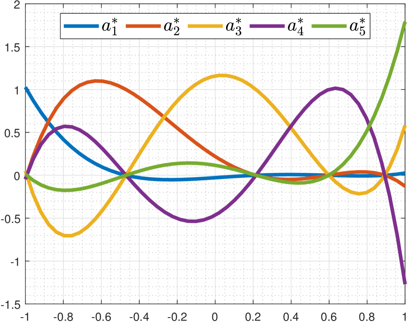
(c) m=4

Figure 1: The weight function $w(x)=e^{-x^{2}}\in\mathcal{C}^{\infty}(\mathbb{R})$, the nodes are $5$ uniformly perturbed equispaced nodes in $[-1,1]$. From left to right the basis functions reproduce the polynomials of degrees $m=0,3$, and $4$ respectively. In this numerical test $\delta=5h_{X,\Omega}$.

Figure 2 points out an interesting aspect of basis functions’ smoothness. [Wen04, Corollary 4.5 ] guarantees a priori that $\{a^{*}_{1},\dots,a^{*}_{5}\}\subseteq\mathcal{C}([-1,1])$ and this is confirmed. But when the degree of the polynomials to be reproduced increases, then also the smoothness of the basis functions increases. We have seen in Theorem 3 that the smoothness of the weight functions does not affect the convergence rate but a smooth approximant can be useful in applications.

To produce Figure 1 and Figure 2 we used the system in equation (9) and as polynomial basis we choose Chebyshev polynomials of the first kind [Riv90].

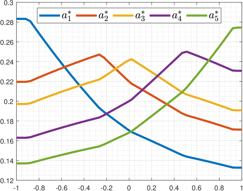
(a) m=0

(b) m=3

(c) m=4

Figure 2: Basis functions of Theorem 4. The weight function coincides with $e^{-x}\in\mathcal{C}(\mathbb{R})$ and the approxiomation nodes are $5$ uniformly perturbed equispaced nodes in $[-1,1]$. From left to right the basis functions reproduce the polynomials of degrees $0,3$ and $4$ respectively. In this numerical test $\delta=5h_{X,\Omega}$.

We continue by analyzing the basis functions of equation (15).

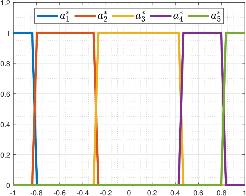
(a) m=0

(b) m=3

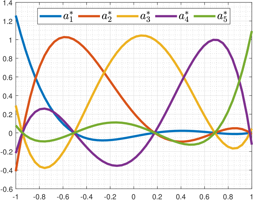
(c) m=4

Figure 3: Basis functions of equation (15). The weight function coincides with $e^{-x^{2}}\in\mathcal{C}^{\infty}(\mathbb{R})$ and the approxiomation nodes are $5$ uniformly perturbed equispaced nodes in $[-1,1]$. From left to right the basis functions reproduce the polynomials of degree $0,3$ and $4$ respectively. In this numerical test $\delta=5h_{X,\Omega}$.

(a) m=0

(b) m=3

(c) m=4

Figure 4: Basis functions of equation (15). The weight function coincides with $e^{-x}\in\mathcal{C}(\mathbb{R})$ and the approxiomation nodes are $5$ uniformly perturbed equispaced nodes in $[-1,1]$. From left to right the basis functions reproduce the polynomials of degree $0,3$ and $4$ respectively. In this numerical test $\delta=5h_{X,\Omega}$.

As fast decaying polynomial reproduction methods Figure 3 and Figure 4 show an interesting result. We do not know the regularity of the basis functions $\{a^{*}_{1},\dots,a^{*}_{5}\}$ but when the degree of the polynomials to be reproduced increases then also the smoothness of the basis functions increases from a practical point of view. With our numerical experiments this consideration does not depend on the weight functions used. We have seen in Theorem 5 that the smoothness of the weight functions does not affect the convergence rate but a smooth approximant can be useful for applications. From Figure 3 and Figure 4 we can underline a characteristic that derives from the method used to solve the linear optimization problem in equation (15). Since we use the simplex method then in each point of $[-1,1]$ only $m+1$ basis functions are different from zero.

To produce Figure 3 and Figure 4 we used as linear optimization solver Gurobi 10 with a tolerance on optimality conditions and constraints of $10^{-10}$. As polynomial basis in equation (18) we choose Chebyshev polynomials of the first kind.

Furthermore, the inclusion of numerical experiments in dimension 2 serves to enhance the introduction of the method in section 5, thereby facilitating a more intuitive understanding.

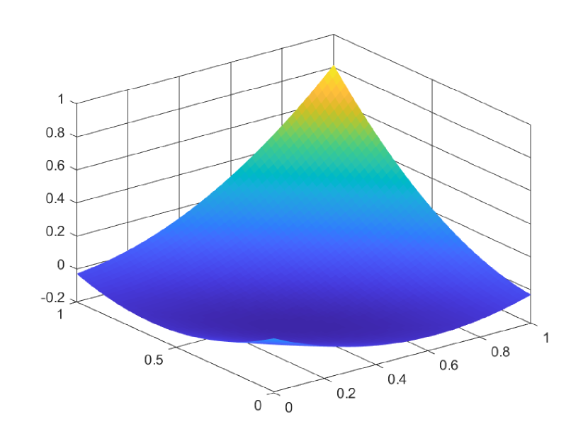
Figure 5: Basis functions of Theorem 4. The weight function coincides with $e^{-x^{2}}\in\mathcal{C}^{\infty}(\mathbb{R})$ and the approxiomation nodes are $9$ equispaced nodes in $[0,1]^{2}$. The basis functions reproduce the polynomials of degree $2$. In this numerical test $\delta=5h_{X,\Omega}$.

To produce Figure 5 we used the system in equation (9) and as polynomial basis we choose standard polynomial basis.

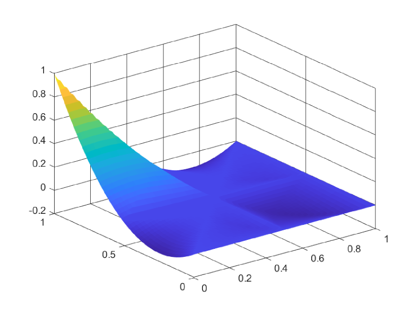
Figure 6: Basis functions of equation (15). The weight function coincides with $e^{-x^{2}}\in\mathcal{C}^{\infty}(\mathbb{R})$ and the approxiomation nodes are $9$ equispaced nodes in $[0,1]^{2}$. The basis functions reproduce the polynomials of degree $2$. In this numerical test $\delta=5h_{X,\Omega}$.

To produce Figure 6 we used as linear optimization solver Gurobi 10 with a tolerance on optimality conditions and constraints of $10^{-10}$. As polynomial basis in equation (18) we choose standard polynomials basis.

As evidenced by the analysis of Figures 3 and 4, the approximation method utilising the minimisation of the 1-norm exhibits a smaller support. Since we exploit the simplex method then in each point of $[0,1]^{2}$ only $\binom{m+2}{2}$ basis functions are different from zero (in this case only $6$ basis functions).

6.2 Numerical Convergence

We discuss some experiments to confirm Theorem 3 numerically. A comprehensive examination of the proposed methodologies for the one-dimensional scenario can be found in [Cap22].

In principle, the proposed approximation methods can be applied whatever the size of the data under consideration. The aforementioned methodologies (equation (6) and equation (15)) have been implemented in a two-dimensional context. We approximate Franke’s bivariate test function (cfr. [FC79]) on equispaced nodes (quasi-uniform data set) in $[0,1]^{2}$. For the method described in equation (6) we use equation (9) to get the approximant and the polynomial basis is the standard polynomial basis. The $1$-norm minimisation method uses the standard polynomial basis and Gurobi 10 with a tollerance of $10^{-10}$ to solve the linear program in equation (18). We fix $\delta=30h_{X,\Omega}$ and we wish to inform that the parameter was defined through a trial and error methodology. Compared to the one-dimensional case, our numerical experiments emphasise that the choice of parameter $\delta$ seems to be more decisive.

As weight function for the two different methods we used

$$w(x,y)=e^{-\left(\frac{|x-y|}{\delta}\right)^{2}}.$$

In the following graphs the blue line allows us to check the correct slope of the approximation error (Theorem 3).

Figure 7: Convergence rate of the approximation error $\|f-z_{f,X}\|_{L^{\infty}([-1,1])}$. The x-axis describes the number of equispaced nodes used to produce the approximant. The approximation method reproduces exactly polynomials of degree $1$.

Nodes	676	729	784	841	900	961	Degree
$e^{-x^{2}}$	1.52e-1	1.43e-1	1.35e-1	1.27e-1	1.20e-1	1.13e-1	1
$\|\cdot\|_{1}-e^{-x^{2}}$	1.68e-2	1.55e-2	1.48e-2	1.35e-2	1.29e-2	9.66e-3	1

Figure 8: Convergence rate of the approximation error $\|f-z_{f,X}\|_{L^{\infty}([-1,1])}$. The x-axis describes the number of equispaced nodes used to produce the approximant. The approximation method reproduces exactly polynomials of degree $2$.

Nodes	676	729	784	841	900	961	Degree
$e^{-x^{2}}$	4.81e-2	4.46e-2	4.14e-2	3.83e-2	3.55e-2	3.29e-2	2
$\|\cdot\|_{1}-e^{-x^{2}}$	1.60e-2	1.41e-2	1.31e-2	1.28e-2	1.26e-2	9.20e-3	2

The previous numerical experiment confirms the statement of Theorem 3 also in a multivariate setting.

6.3 Basis functions with algebraic decay

As demonstrated in equation (10), Shepard’s method represents a specific instance of the proposed numerical schemes. It is therefore advantageous to study basis functions with algebraic decay.

In this section, we assume that

$$\varphi(x)\leq\frac{1}{x^{k}}\quad\text{ for }\,x\in\mathbb{R}_{>0}\quad\textrm{ and }\quad k\in\mathbb{R}_{>0}.$$ (26)

In this case, $\varphi$ may diverge in $0^{+}$ and fail the ratio test (cfr. Definition 4). We have shown that the convergence of the Fast-Decaying Polynomial Reproduction framework (Theorem 3) depends on inequality (4).

From inequalities

$$|u_{j}(x)|\leq C\varphi\left(\frac{\|x-x_{j}\|_{2}}{q_{X}}\right)\leq C\frac{q_{X}^{k}}{\|x-x_{j}\|_{2}^{k}}\;\text{ for all }\;x\in\Omega\;\text{ and }\;j=1,\dots,N$$

we can derive the inequality (4) with a different value for $K$ (the proof retraces the steps of Theorem 5, but we need to use algebraic decay when studying the nodes distributions in the set $E_{0}$).
The choice of the exponent $k$ in (26) is crucial for the convergence and stability of the method: if the method reproduces polynomials up to degree $m$ in $\mathbb{R}^{d}$ then $d+m-\frac{k}{2}<-1$ (moving least squares) or $d+m-k<-1$ (approximation with the $1$-norm). We obtained this result using equations (14) and (17) with the convergence of the generalized harmonic series. These constraints on the exponent $k$ are consistent with those found in [LC92]. Indeed there exists $\lambda\in]0,1[$ such that, in a neighborhood of $+\infty$ that does not contain $0$, say for instance $]1,+\infty[$

$$\sup_{x\in]1,+\infty[}\left\{|\varphi(x)|(1+x)^{d+m+1+\lambda}\right\}<+\infty.$$

Concerning algebraic decay, the aforementioned schemes mimic the construction presented in [LC92], and they extend that construction to incorporate divergence in $0^{+}$. Another advantage of our framework is that it permits to validate the regularity of the approximant with the smoothness of the basis functions, thereby extending the scope of applicability beyond that of continuous functions with algebraic decay.

As test function for the two different methods (moving least squares and approximation with linear programming) we used

$$f(x)=\sin(\pi x).$$

(a) $k=6.2$

(b) $k=3.1$

Figure 9: Convergence rate of the approximation error $\|f-z_{f,X}\|_{L^{\infty}([-1,1])}$. The x-axis describes the number of equispaced nodes used to produce the approximant. The approximation method reproduces exactly polynomials of degree $1$. In this numerical test $\delta=5h_{X,\Omega}$.

Nodes	8	16	32	64	Degree
MLS	5.61e-01	1.01e-01	2.02e-02	5.07e-03	1
$\|\cdot\|_{1}$	6.82e-02	1.52e-02	4.41e-03	9.31e-04	1

6.4 Stability

The objective of this section is to numerically verify the Lebesgue constant and the stability of the approximation methods that have been the subject of this study. Theorem 5 allows the estimation of the Lebesgue constant to be made without dependence on the parameters in equations (2) and (3). We fix $\delta=5h_{X,\Omega}$.

As weight function we used

$$w(x,y)=e^{-\left(\frac{|x-y|}{\delta}\right)^{2}}.$$

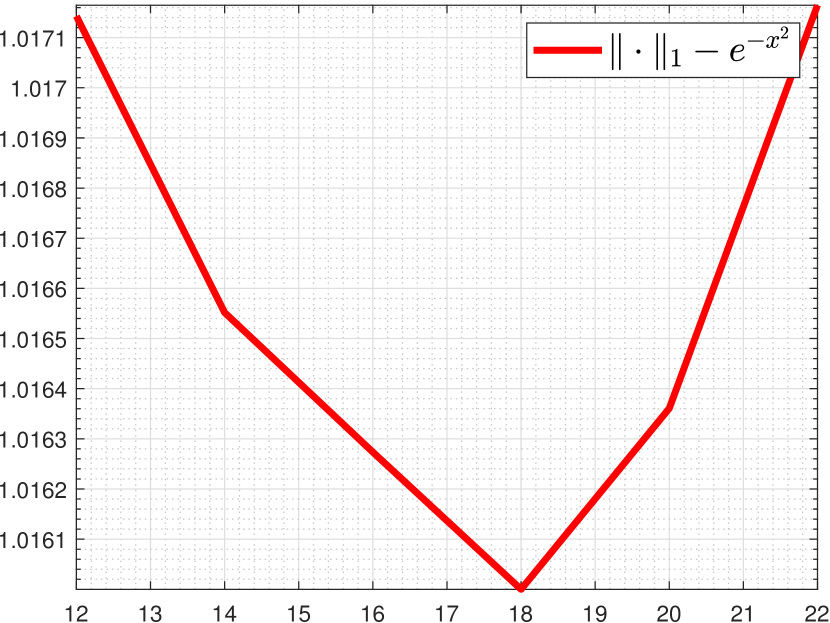
Figure 10: Lebesgue constants of the methods in equation (6) and in equation (15) respectively. The x-axis describes the number of equispaced nodes used to produce the basis functions. The approximation methods reproduces exactly polynomials of degree $2$.

Nodes	169	225	289	361	441	529	Degree
$e^{-x^{2}}$	2.203275	2.173473	2.155158	2.142972	2.136264	2.133485	2
$\|\cdot\|_{1}-e^{-x^{2}}$	1.017143	1.016552	1.016274	1.016000	1.016361	1.017165	2

7 Conclusion

The rescaled localized radial basis function method (RL-RBF) proposed in [DFQ14] represents an efficient numerical scheme to interpolate functions on a scattered set of nodes. We have to wait for the results of [DW20] to read a proof of the convergence for RL-RBF: this proof works up to a conjecture in the quasi-uniform setting.

Our work continues from this generalizing the RL-RBF method by increasing the dimension of the polynomial space to be reproduced exactly. The goal is to determine a convergent method whose convergence rate is $\mathcal{O}(h_{X,\Omega}^{m+1})$ if all polynomials up to degree $m$ can be approximated correctly. We modified the definition of local polynomial reproduction by replacing the compactness of the support with a fast decay of the basis functions. The RL-RBF method adapts to this new definition, while it does not reproduce polynomials locally because the cardinal functions do not have compact support. In the quasi-uniform setting this new approximation scheme is convergent and stable (the Lebesgue constant depends on the dimension of the space, the dimension of the polynomial space that is reproduced and on the decaying of the basis functions). At this point in the analysis, smoothness plays no fundamental role. In addition to RL-RBF method, we proposed a further approximation scheme that provides smooth quasi-interpolants. The method approximates the value of an unknown function using the moving least squares technique with a Gaussian as weight function. The smoothness of the interpolant is inherited from the smoothness of the weight functions. Since the solution of a moving least squares problem is the solution of a quadratic optimization problem we can analyze the computational cost of the method, which turns out to be linear in the number of nodes. Numerical tests confirm the theoretical results of convergence, stability and also the smoothness of the basis functions. With the numerical tests we obtain an unexpected result: even if the weight function is only continuous, if we increase the dimension of the polynomial space to be reproduced then the basis functions turn out to be numerically smooth.

In these analysis and numerical tests we considered functions with global support and the matrices involved can be dense although small in size when the space to be reproduced is not too large. To address this difficulty we replaced the quadratic optimization problem deriving from moving least squares with a linear program on a polyhedron. Also in this area, with techniques similar to the previous ones, a stable and convergent method can be achieved with the same convergence rate. A vertex solution of the linear optimization problem allows us to control the number of non-zero basis functions at each point in the domain. Since the weight functions try to locate the optimization problem, we expect that the value of the weight function corresponding to a node in the domain is large when the considered point is far from the node. This type of experience leads us to use column generation techniques to reduce the dimensionality of the problem (we can try to predict the non-zero basis functions because the number of them is bounded uniformly with respect to the fill distance). The numerical results confirm the theoretical evidence and even if we do not have any results on the smoothness of the approximant we get similar outcomes to the moving least squares method (numerically we can observe that the basis functions become smooth when the polynomial space is reproduced gets bigger). The methods have also been subjected to multivariate testing. We have also experimented with degenerate basis functions (algebraic decay and divergent at $0^{+}$). The numerical results confirm the framework’s validity, but the exponent’s choice is crucial to achieving stability and convergence.

In the future, we intend to extend the applicability of Fast-Decaying Polynomial Reproduction schemes to more general point distributions by utilizing the Fake Nodes Approach [De ̵+21]. Another line of research refers to the optimality of the Lebesgue constant in equation (5). Indeed, by tuning the parameters $C$ and $\varphi$ it is possible to reach better stability and obtain optimal controls for the decay of the basis functions.

Acknowledgments.

This work started during an Erasmus traineeship at the University of Bayreuth under the supervision of prof. Holger Wendland. Both authors are very grateful for instructive discussions with prof. Martin Buhmann of the University of Giessen. This research has been achieved as part of RITA “Research ITalian network on Approximation” and as part of the UMI topic group “Teoria dell’Approssimazione e Applicazioni”. The authors are also members of the INdAM-GNCS Research group.

References

- [BJ22] Martin Buhmann and Janin Jäger “Quasi-Interpolation”, Cambridge Monographs on Applied and Computational Mathematics Cambridge University Press, 2022
- [Cap22] Giacomo Cappellazzo “Rescaled localized radial basis functions and fast decaying polynomial reproduction” In Padua Thesis and Dissertation Archive, 2022 URL: https://hdl.handle.net/20.500.12608/52238
- [CCZ14] Michele Conforti, Gerard Cornuejols and Giacomo Zambelli “Integer Programming” Springer Publishing Company, Incorporated, 2014
- [De ̵+21] S. De Marchi, F. Marchetti, E. Perracchione and D. Poggiali “Multivariate approximation at fake nodes” In Applied Mathematics and Computation 391, 2021, pp. 125628 DOI: https://doi.org/10.1016/j.amc.2020.125628
- [DW20] Stefano De Marchi and Holger Wendland “On the convergence of the rescaled localized radial basis function method” In Applied Mathematics Letters 99, 2020, pp. 105996 DOI: https://doi.org/10.1016/j.aml.2019.105996
- [DFQ14] Simone Deparis, Davide Forti and Alfio Quarteroni “A Rescaled Localized Radial Basis Function Interpolation on Non-Cartesian and Nonconforming Grids” In SIAM Journal on Scientific Computing 36.6, 2014, pp. A2745–A2762 DOI: 10.1137/130947179
- [Fas07] Gregory F. Fasshauer “Meshfree Approximation Methods with MATLAB” USA: World Scientific Publishing Co., Inc., 2007
- [Fly06] N. Flyer “Exact polynomial reproduction for oscillatory radial basis functions on infinite lattices” In Computers & Mathematics with Applications 51.8, 2006, pp. 1199–1208 URL: https://www.sciencedirect.com/science/article/pii/S0898122106000733
- [FC79] R. Franke and NAVAL POSTGRADUATE SCHOOL MONTEREY CA. “A Critical Comparison of Some Methods for Interpolation of Scattered Data”, Final report Defense Technical Information Center, 1979 URL: https://books.google.it/books?id=ZgQ5HAAACAAJ
- [Kar08] H. Karloff “Linear Programming”, Modern Birkhäuser Classics Birkhäuser Boston, 2008 URL: https://books.google.it/books?id=Sld1YYAedtgC
- [LS81] Peter Lancaster and Kestutis Salkauskas “Surfaces generated by moving least squares methods” In Mathematics of Computation 37, 1981, pp. 141–158
- [LC92] W.A. Light and E.W. Cheney “Quasi-interpolation with translates of a function having noncompact support” In Constr. Approx. 8.1, 1992, pp. 35–48 URL: https://link.springer.com/article/10.1007/BF01208904
- [MS96] V. Maz’ya and G. Schmidt “On approximate approximations using Gaussian kernels” In IMA J. Numer. Anal. 16.1, 1996, pp. 13–29 URL: https://www.scopus.com/record/display.uri?eid=2-s2.0-0039863907&origin=reflist
- [McL74] D.. McLain “Drawing Contours from Arbitrary Data Points” In Comput. J. 17, 1974, pp. 318–324
- [McL76] D.. McLain “Two Dimensional Interpolation from Random Data” In Comput. J. 19, 1976, pp. 178–181 URL: https://api.semanticscholar.org/CorpusID:37308780
- [Riv90] T.J. Rivlin “Chebyshev Polynomials: From Approximation Theory to Algebra and Number Theory”, Pure and Applied Mathematics: A Wiley Series of Texts, Monographs and Tracts Wiley, 1990 URL: https://books.google.it/books?id=plTvAAAAMAAJ
- [Sch97] Robert Schaback “Reproduction of polynomials by radial basis functions” In ResearchGate, 1997 URL: https://www.researchgate.net/publication/2290667_Reproduction_of_Polynomials_by_Radial_Basis_Functions
- [She68] Donald Shepard “A Two-Dimensional Interpolation Function for Irregularly-Spaced Data” In Proceedings of the 1968 23rd ACM National Conference, ACM ’68 New York, NY, USA: Association for Computing Machinery, 1968, pp. 517–524 DOI: 10.1145/800186.810616
- [Str70] G. Strang “The finite-element method and approximation theory.” In Numerical Solution of Partial Differential Equations (B. Hubbard, ed.), SYNSPADE 1970, University of Maryland, 1970, pp. 547–583
- [Wen01] Holger Wendland “Local polynomial reproduction and moving least squares approximation” In Ima Journal of Numerical Analysis 21, 2001, pp. 285–300 URL: https://api.semanticscholar.org/CorpusID:120212734
- [Wen04] Holger Wendland “Scattered Data Approximation”, Cambridge Monographs on Applied and Computational Mathematics Cambridge University Press, 2004 DOI: 10.1017/CBO9780511617539