Effects of heavy quarks in the dipole cross section with the KLN model

Abstract

The dipole cross-section behavior for protons and nuclei is analyzed with and without considering the heavy quark masses in the Bjorken variable $x$ using the Kharzeev-Levin-Nardi (KLN) model of low $x$ gluon distributions. The Color Glass Condensate (CGC) effects in the color dipole model are influenced by the heavy quark masses in the Bjorken variable $x$ at $Q^{2}<Q_{s}^{2}$. These non-linear saturation effects will be observable in the LHeC and EIC at very small $x$ values.

.1 I. Introduction

The saturation model is particularly intriguing when describing deep inelastic scattering (DIS) data at low $x$, as the saturation of the growth of gluon densities in hadrons and nuclei is evident in this region Ref1 ; Ref2 ; Ref3 ; Ref4 . A simple model by Kharzeev, Levin, and Nardi (KLN) in Ref.Ref5 was proposed to explain saturation physics for the unintegrated gluon distribution function. This model only provides an Ansatz for the gluon distribution function, which is suitable for color dipole models modified into the gluon density. Hadron physics in new accelerators, such as LHeC and EIC, relies on the saturation scale, $Q_{s}^{2}$, in the KLN model which is interpreted as evidence for parton recombination and saturation.
A new regime of quantum chromodynamics (QCD) is characterized by high gluon densities at $Q^{2}<Q_{s}^{2}$. In this regime, gluon densities at small $x$, in a hadron wavefunction, represent the Color Glass Condensate (CGC) Ref6 ; Ref7 . The boundary between dense and dilute gluonic systems is related to the presence of large quark masses in the Bjorken variable $x$. In this paper, we demonstrate that the non-linear saturation dynamics incorporated into the CGC model are observable when using the Bjorken scaling for the proton color dipole cross section at very small $x$, but are eliminated when the Bjorken variable depends on charm and bottom quark masses. For light and heavy nuclei, the non-linear saturation dynamics are apparent at very small $x$ when considering the modified Bjorken variable $x$.

.2 II. Dipole cross section

The proton structure function $F_{2}$ is related to the $\gamma^{*}p$ cross section as

$$F_{2}(x,Q^{2})=\frac{Q^{2}}{4\pi^{2}\alpha_{em}}\bigg{(}\sigma^{\gamma^{*}p}_{T}(x,Q^{2})+\sigma^{\gamma^{*}p}_{L}(x,Q^{2})\bigg{)}.$$ (1)

In the color dipole picture (CDP), the scattering between the virtual photon $\gamma^{*}$ and the proton is seen in the following form

$$\sigma_{L,T}^{\gamma^{*}p}(x,Q^{2})=\int dzd^{2}\mathbf{r}|\Psi_{L,T}(\mathbf{r},z,Q^{2})|^{2}\sigma_{\mathrm{dip}}(\widetilde{{x}},\mathbf{r}).$$ (2)

The virtual photon dissociates into a quark-antiquark pair (a $q\overline{q}$ dipole) which interacts with the color fields in the proton. The imaginary part of the $(q\overline{q})p$ forward scattering amplitude is defined by the dipole cross-section, $\sigma_{\mathrm{dip}}({x},r)$. The variables $r$ and $z$ are defined, with respect to the photon momentum, representing the transverse dipole size and the longitudinal momentum fraction respectively Ref1 ; Ref2 ; Ref3 ; Ref4 . $\Psi_{L,T}$ is the photon wave function with respect to the photon polarization and depends on the mass of the quarks in the $q\overline{q}$ dipole. Therefore, the Bjorken variable $x$ is modified by the following form Ref8

$$x{\rightarrow}\widetilde{x}_{f}=x\bigg{(}1+\frac{4m_{f}^{2}}{Q^{2}}\bigg{)},$$ (3)

where $m_{f}$ is the quark mass.
The dipole cross-section in the Golec-Biernat and W$\mathrm{\ddot{u}}$sthoff (GBW) model Ref4 , depends on the dipole size $r$ and the saturation scale $Q_{\mathrm{sat}}(x)$ as follows

$$\sigma_{\mathrm{dip}}(\widetilde{x},\mathbf{r})=\sigma_{0}\bigg{\{}1-\exp\bigg{(}-r^{2}Q_{\mathrm{sat}}^{2}(\widetilde{x})/4\bigg{)}\bigg{\}},$$ (4)

where the saturation scale is parametrized as $Q_{\mathrm{sat}}^{2}(\widetilde{x})=Q_{0}^{2}(x_{0}/\widetilde{x})^{\lambda}$. The dipole cross section was improved by taking into account the evolution of the gluon density in Ref.Ref9 . The modified dipole cross section in the Bartels, Golec-Biernat and Kowalski (BGK) model Ref9 reads

$$\sigma_{\mathrm{dip}}(\widetilde{x},\mathbf{r})=\sigma_{0}\bigg{\{}1-\exp\bigg{(}-\frac{\pi^{2}r^{2}\alpha_{s}(\mu^{2})xg(\widetilde{x},\mu^{2})}{3\sigma_{0}}\bigg{)}\bigg{\}},$$ (5)

where the evolution scale $\mu^{2}$ is connected to the size of the dipole by $\mu^{2}=\frac{C}{r^{2}}+\mu^{2}_{0}$.
In the following we shall use the KLN Ansatz Ref10 in the dipole cross section in the following form

$$\sigma_{\mathrm{dip}}(\widetilde{x},\mathbf{r}) = \sigma_{0}\bigg{\{}1-\exp\bigg{(}-\frac{\pi^{2}r^{2}\alpha_{s}(\mu^{2})}{3\sigma_{0}}\bigg{[}$$ (6)

$$\frac{K_{0}S}{\alpha_{s}(Q_{s}^{2})}\mu^{2}(1-x)^{D}\Theta(Q_{s}^{2}-\mu^{2})$$

$$+\frac{K_{0}S}{\alpha_{s}(Q_{s}^{2})}Q_{s}^{2}(1-x)^{D}\Theta(\mu^{2}-Q_{s}^{2})\bigg{]}\bigg{)}\bigg{\}},$$

where $S$ is the area of the target and $K$ is a constant parameter obtained from the momentum sum rule. The nuclear dipole cross section $\sigma^{A}_{\mathrm{dip}}$ with the KLN distribution can accurately predict data from deep inelastic scattering in electron-ion collisions (EICs) Ref11 ; Ref12 ; Ref13 . For a nuclear target with the mass number A, the nuclear dipole cross section remains the same for the change $xg(x,Q^{2}){\rightarrow}xg^{A}(x,Q^{2})$ as

$$\sigma^{A}_{\mathrm{dip}}(\widetilde{x},\mathbf{r}) = \sigma^{A}_{0}\bigg{\{}1-\exp\bigg{(}-\frac{\pi^{2}r^{2}\alpha_{s}(\mu^{2})}{3\sigma^{A}_{0}}\bigg{[}$$ (7)

$$\frac{K_{0}S_{A}}{\alpha_{s}(Q_{sA}^{2})}\mu^{2}(1-x)^{D}\Theta(Q_{sA}^{2}-\mu^{2})$$

$$+\frac{K_{0}S_{A}}{\alpha_{s}(Q_{sA}^{2})}Q_{sA}^{2}(1-x)^{D}\Theta(\mu^{2}-Q_{sA}^{2})\bigg{]}\bigg{)}\bigg{\}},~{}~{}~{}$$

where the replacements are $S^{A}=A^{2/3}S$, $\sigma_{0}^{A}=A^{2/3}\sigma_{0}$ and $Q^{2}_{sA}=A^{1/3}Q^{2}_{s}$ Ref10 ; Ref14 .
By considering the individual quark flavor pairs in the QCD dipole picture, the rescaling Bjorken variable $x$ (i.e., Eq.(3)) is modified from light quark pairs to heavy quark pairs (i.e., $c\overline{c}$ and $b\overline{b}$ pairs). Indeed the rescaling variable $\widetilde{x}_{f}=x{(}1+\frac{4m_{f}^{2}}{\mu^{2}}{)}$ is introduced Ref15 to extend the saturation model to the low $\mu^{2}$ (large $r$) region including the photoproduction limit. The dipole cross sections for nucleons and nuclei (i.e., Eqs.(6) and (7)) in the KLN model satisfy the condition of $Q^{2}>Q^{2}_{sA}$ (for proton A=1) when the rescaling Bjorken variable $x$ is considered. Without the rescaling variable, the dipole cross section behavior will deviate from the GBW model when it satisfies the condition $Q^{2}<Q^{2}_{sA}$ at large $r$. This deviation is supported by the CGC model Ref16 ; Ref6 ; Ref7 . In the next section we will consider the behavior of the dipole cross section with and without the rescaling effects for nucleons and nuclei. Indeed, the rescaling effect is one of the ingredients used in the general-mass variable flavor number schemes (GM-VFNS) Ref17 .

.3 II. Results and Conclusions

The fixed parameters are summarized in Table I for the quark masses of Fits 0, 1 and 2 with the quark masses $m_{l}=0.14~{}\mathrm{GeV}$, $m_{c}=1.4~{}\mathrm{GeV}$ and $m_{b}=4.6~{}\mathrm{GeV}$ respectively, as shown in Ref.Ref5 . We have calculated the $r$-dependence of the ratio $\sigma_{\mathrm{dip}}/\sigma_{0}$ (i.e., Eq.(6)) based on the KLN model for $x=10^{-6}$ and $10^{-3}$. In Figs.1 and 2, the results of the KLN model are compared with the GBW model, considering the charm and bottom masses in the rescaling variable $x$, respectively. The coefficients in the CDP are based on fits 1 and 2 in Table I, as shown in Figs.1 and 2 respectively. The rescaling variable $x$ (i.e., Eq.(3)) is applied to the GBW and KLN models as we observe that the results are comparable in these figures (i.e., Figs.1 and 2). In wide ranges of $x$ and $r$, the KLN results fall within the domain $\mu^{2}>Q_{s}^{2}$ when we consider the rescaling variable with charm and bottom masses. Indeed, the rescaling variable ensures the GM-VFNS in the KLN model.

Table 1: The fixed parameters of the color dipole model from the fit results in Ref.Ref8 .

Fit	C	$\mu_{0}^{2}~{}[\mathrm{GeV}^{2}]$	$\sigma_{0}~{}[\mathrm{mb}]$	$\lambda$	$x_{0}{\times}10^{-4}$
0	0.29	1.85	23.58	0.270	2.24
1	0.29	1.85	27.32	0.248	0.42
2	0.27	1.74	27.43	0.248	0.40

The ratio $\sigma_{\mathrm{dip}}/\sigma_{0}$ in the KLN model is calculated without considering the charm and bottom masses in Figs.3 and 4. Without the rescaling variable $x$, the hard saturation momentum $Q_{s}(x)$ grows rapidly as $x$ decreases at large values of $r$. In Figs.3 and 4, we observe that the condition $\mu^{2}>Q^{2}_{s}$ is valid at small $r$, and the condition $\mu^{2}<Q^{2}_{s}$ at large $r$ is valid. For $\mu^{2}<Q^{2}_{s}$ at large $r$ the saturation becomes visible. The deviations of the ratio $\sigma_{\mathrm{dip}}/\sigma_{0}$ from a straight line at low $x$ values (specifically at $x=10^{-6}$), indicate the significance of non-linear effects in the KLN model without the rescaling variable. In reality, saturation effects are only noticeable at very small $x$ ($x=10^{-6}$) and for large values of $r$. This depletion in the ratio is referred to as shadowing. The depletion point increases towards larger $r$ with an increase in the production of heavy quarks from $c\overline{c}$ to $b\overline{b}$ in the CDP. For the production of $c\overline{c}$ in the CDP this depletion point is at $r>0.06$ in Fig.3 and at $r>0.1$ for the production of $b\overline{b}$ in Fig.4.

Figure 1: The extracted ratio $\sigma_{\mathrm{dip}}/\sigma_{0}$ as a function of $r$ for $x=10^{-6}$ (brown curve) and $x=10^{-3}$ (blue curve) (curves are from left to right, respectively) using the KLN model, Eq.(6), compared with the GBW model (solid curves), Eq.(4). In these results the charm effect in the rescaling Bjorken variable $x$ (i.e., Eq.(3)) is considered. The coefficients are based on the results from Fit 1 in Table I.

Figure 2: The extracted ratio $\sigma_{\mathrm{dip}}/\sigma_{0}$ as a function of $r$ for $x=10^{-6}$ (brown curve) and $x=10^{-3}$ (blue curve) (curves are from left to right, respectively) using the KLN model, Eq.(6), compared with the GBW model (solid curves), Eq.(4). In these results the bottom effect in the rescaling Bjorken variable $x$ (i.e., Eq.(3)) is considered. The coefficients are based on the results from Fit 2 in Table I.

Figure 3: The extracted ratio $\sigma_{\mathrm{dip}}/\sigma_{0}$ as a function $r$ for $x=10^{-6}$ (brown curve) and $x=10^{-3}$ (blue curve) (curves are from left to right, respectively) with the KLN model, Eq.(6) without the charm effect in the rescaling Bjorken variable $x$. The coefficients are based on the results from Fit 0 in Table I.

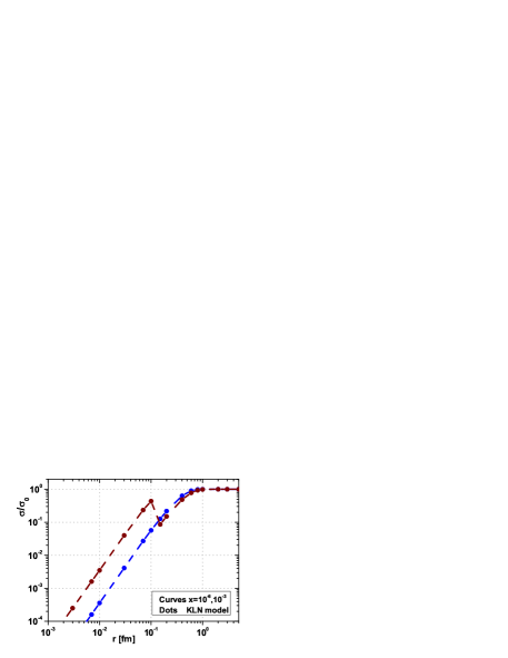
Figure 4: The extracted ratio $\sigma_{\mathrm{dip}}/\sigma_{0}$ as a function $r$ for $x=10^{-6}$ (brown curve) and $x=10^{-3}$ (blue curve) (curves are from left to right, respectively) with the KLN model, Eq.(6) without the bottom effect in the rescaling Bjorken variable $x$. The coefficients are based on the results from Fit 1 in Table I.

It is interesting that the dipole cross sections in Figs.3 and 4 have a property of geometrical scaling, without the rescaling Bjorken variable $x$. This means they become independent of $x$ and $r$ at large $r$. The KLN criterion is a border between dense and dilute gluonic systems, which is defined by the geometrical scaling and is observable with and without the rescaling variable in the dipole cross sections Ref18 .
In nuclear targets, non-linear effects in electron-nucleus (eA) processes are evident even when rescaling the Bjorken variable in the dipole cross sections due to the KLN model. The KLN prescription for the CGC dynamics is discussed in Ref.Ref19 . This saturation refers to the very small-$x$ evolution effects in the dipole cross sections and will be one of the key physics goals of an Electron-Ion Collider.
The ratio $\sigma^{A}_{\mathrm{dip}}/\sigma^{A}_{0}$ for the light and heavy nucleus of C-12 and Pb-208 as a function of $r$ with respect to the rescaling of the Bjorken variable with charm mass effect for $x=10^{-3}$ and $10^{-6}$ is shown in Figs.5 and 6 respectively.

Figure 5: The extracted ratio $\sigma_{\mathrm{dip}}/\sigma_{0}$ for C-12 as a function of $r$ for $x=10^{-6}$ (brown curve) and $x=10^{-3}$ (blue curve) (curves are from left to right, respectively) using the KLN model, Eq.(4). In these results the charm effect in the rescaling Bjorken variable $x$ (i.e., Eq.(3)) is considered. The coefficients are based on the results from Fit 1 in Table I.

Figure 6: The same as Fig.5 for Pb-208.

In Figs.7 and 8, the ratio $\sigma^{A}_{\mathrm{dip}}/\sigma^{A}_{0}$ for the light and heavy nucleus of C-12 and Pb-208 as a function of $r$ with respect to the rescaling of the Bjorken variable with bottom mass effect for $x=10^{-3}$ and $10^{-6}$ is shown respectively.

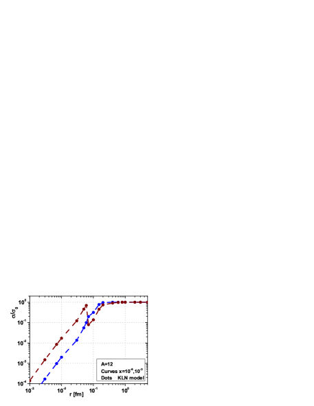
Figure 7: The extracted ratio $\sigma_{\mathrm{dip}}/\sigma_{0}$ for C-12 as a function of $r$ for $x=10^{-6}$ (brown curve) and $x=10^{-3}$ (blue curve) (curves are from left to right, respectively) using the KLN model, Eq.(4). In these results the bottom effect in the rescaling Bjorken variable $x$ (i.e., Eq.(3)) is considered. The coefficients are based on the results from Fit 2 in Table I.

Figure 8: The same as Fig.7 for Pb-208.

The deviation of the ratios $\sigma^{A}_{\mathrm{dip}}/\sigma^{A}_{0}$ at very low $x$ (i.e., $x=10^{-6}$) in Figs.5-8 shows the importance of non-linear effects in the KLN model in EICs. Indeed, saturation effects due to the rescaling variable are noticeable at very low values of $x$ and for large values of the dipole size $r$. This saturation by the KLN model will be visible in EICs as described in Ref.Ref20 by the b-CGC model.
The non-linear effects caused by the charm effects in the rescaling Bjorken variable $x$ at $x=10^{-6}$ are visible in Fig.5 for the light nucleus of C-12 at $r{\gtrsim}0.04$ and in Fig.6 for the heavy nucleus of Pb-208 at $r{\gtrsim}0.02$ respectively. Depletions observed in Figs.5 and 6 clearly demonstrate shadowing effects in the EICs at very low $x$ and large $r$. It is important to emphasize that the non-linear effects are not visible at small $x$ (i.e., $x{\approx}10^{-3}$).
In Figs.7 and 8 the non-linear effects caused by the bottom effects in the rescaling Bjorken variable $x$ at $x=10^{-6}$ are observable for the light nucleus of C-12 at $r{\gtrsim}0.06$ and for the heavy nucleus of Pb-208 at $r{\gtrsim}0.04$ respectively. The scale $r$ for the non-linear effects for light and heavy nuclei increases as the heavy quark mass effect at the rescaling variable increases from charm to bottom masses. We observe that, in Figs.6 and 8, depletion of the non-linear effects for heavy nuclei is deeper than those for light nuclei in Figs.5 and 7 at very low $x$ and large $r$. We observe that significant non-linear effects begin to appear at smaller values of $x$ for heavy nuclei Ref21 ; Ref22 ; Ref23 .

In conclusion, we have considered the non-linear saturation effects in the dipole cross section using the KLN model while also accounting for heavy quark masses in the Bjorken variable $x$. This approach demonstrates the CGC model in the color dipole cross section for both protons and nuclei at very low values of the Bjorken variable $x$. The $Q^{2}_{s}$ dependence of $\sigma_{\mathrm{dip}}$ more accurately determined with and without consideration of the charm and bottom masses in the dipole model. We anticipate that the observable effects of non-linear saturation will be seen in the LHeC and EIC accelerators.

.4 ACKNOWLEDGMENTS

G.R.Boroun would like to thank Professor F.S. Navarra for useful comments and invaluable support.

References

- (1) N.N. Nikolaev, B.G. Zakharov, Z. Phys. C 49, 607 (1991).
- (2) N.N. Nikolaev, B.G. Zakharov, Z. Phys. C 53, 331 (1992).
- (3) N. N. Nikolaev and W. Schfer, Phys. Rev. D 74, 014023 (2006).
- (4) K.Golec-Biernat and M.Wsthoff, Phys. Rev. D 59, 014017 (1998).
- (5) D. Kharzeev, E. Levin and M. Nardi, Phys. Rev. C71, 054903 (2001); Nucl. Phys. A 730, 448 (2004); Nucl. Phys. A 747, 609 (2005).
- (6) E.Ferreiro, E.Iancu, A.Leonidov and L.McLerran, Nucl.Phys.A 703, 489 (2002).
- (7) E.Iancu, K.Itakura and S.Munier, Phys.Lett.B 590, 199 (2004).
- (8) K. Golec-Biernat and S.Sapeta, JHEP 03, 102 (2018).
- (9) J.Bartels, K.Golec-Biernat and H.Kowalski, Phys. Rev. D66, 014001 (2002).
- (10) F.Carvalho, F.O.Dures, F.S.Navarra and S.Szpigel, Phys.Rev.C 79, 035211 (2009).
- (11) R. Abdul Khalek et al., Snowmass 2021 White Paper, arXiv [hep-ph]:2203.13199.
- (12) . R.Abir et al., The case for an EIC Theory Al- liance: Theoretical Challenges of the EIC, arXiv [hep-ph]:2305.14572.
- (13) LHeC Collaboration, FCC-he Study Group, P. Agostini, et al., J. Phys. G, Nucl. Part. Phys. 48, 110501 (2021).
- (14) J. Rausch, V. Guzey and M. Klasen, Phys. Rev. D 107, 054003 (2023).
- (15) A.M.Stasto, K. Golec-Biernat and J.Kwiecinski, Phys.Rev.Lett. 86, 596 (2001).
- (16) E.Iancu, A.Leonidov and L.McLerran, Nucl.Phys.A 692, 583 (2001); Phys.Lett.B 510, 133 (2001).
- (17) G.Beuf, C.Royon and D.Salek, arXiv:hep-ph/0810.5082(2008).
- (18) T.Stebel, Phys.Rev.D 88, 014026 (2013).
- (19) W.A.Horowitz, arXiv [hep-ph]:1102.5058.
- (20) E. R. Cazaroto, F. Carvalho, V. P. Goncalves and F. S. Navarra, Phys. Lett. B 671, 233 (2009).
- (21) Yuri V.Kovchegov, H.Sun and Z.Tu, Phys.Rev.D 109, 094028 (2024).
- (22) B.Z.Kopeliovich, I.K.Potashnikova, and I.Schmidt, Phys.Rev.C 81, 035204 (2010).
-
(23)
B.Z. Kopeliovich, arXiv[hep-ph]:1602.00298.