The non-equilibrium Marshak wave problem in non-homogeneous media

Abstract

We derive a family of similarity solutions to the nonlinear non-equilibrium Marshak wave problem for an inhomogeneous planar medium which is coupled to a time dependent radiation driving source. We employ the non-equilibrium gray diffusion approximation in the supersonic regime. The solutions constitute a generalization of the non-equilibrium nonlinear solutions that were developed recently for homogeneous media. Self-similar solutions are constructed for a power law time dependent surface temperature, a spatial power law density profile and a material model with power law temperature and density dependent opacities and specific energy density. The extension of the problem to non-homogeneous media enables the existence of similarity solutions for a general power law specific material energy. It is shown that the solutions exist for specific values of the temporal temperature drive and spatial density exponents, which depend on the material exponents. We also illustrate how the similarity solutions take various qualitatively different forms which are analyzed with respect to various parameters. Based on the solutions, we define a set of non-trivial benchmarks for supersonic non-equilibrium radiative heat transfer. The similarity solutions are compared to gray diffusion simulations as well as to detailed implicit Monte-Carlo and discrete-ordinate transport simulations in the optically-thick regime, showing a great agreement, which highlights the benefit of these solutions as a code verification test problem.

I Introduction

The theory of radiation hydrodynamics is at the heart of various high energy density systems, such as inertial confinement fusion and astrophysical phenomena [1, 2, 3, 4, 5, 6, 7]. Analytic solutions for the equations of radiation hydrodynamics are an important and practical aspect of the analysis and design of high energy density experiments [8, 9, 10, 5, 11, 12, 13, 14] and are frequently used for the verification of computer simulations [15, 16, 17, 18, 19, 20, 21, 22, 23, 24, 25, 26, 27, 28, 29].

The theory of Marshak waves which was developed in the seminal work [30] and was further generalized in Refs. [31, 32, 33, 34, 35, 36, 16, 37, 38, 39, 40, 41, 42, 43, 10, 28], is a fundamental phenomena that describes the nonlinear propagation of radiation and the subsequent thermalization of a material that is illuminated by an intense radiation energy source. In most cases, radiative heat conduction plays a pivotal role in the process. At high temperatures and for non-opaque materials, the radiative heat wave may propagate faster than the speed of sound, resulting in a supersonic Marshak wave [38, 39, 44, 42, 45, 46, 12, 27, 28], for which the material motion is negligible.

Originally, the Marshak wave problem was addressed under the assumption of local thermodynamic equilibrium between the radiation field and the heated material. This scenario is only valid for systems which are optically thick with respect to the emission-absorption process. Pomraning and subsequently Su and Olson, in their seminal works [47, 48], derived a widely used [49, 50, 51, 52, 53, 54, 55, 56, 57, 58] solution for a non-equilibrium linear Marshak wave problem in the diffusion limit of radiative transfer, assuming a temperature independent opacity, a material energy density that depends on temperature as $\sim T^{4}$ and a spatially homogeneous media. This solution was further extended, yet in the linear regime, in Refs. [59, 60, 61, 62, 63]. However, opacities of real materials usually depend strongly on temperature, so that nonlinear conduction prevails in most high-energy-density systems. Recently, in Ref. [27], a family of new solutions to the non-equilibrium Marshak wave problem was developed for nonlinear conduction scenarios. These solutions were developed by employing a dimensional analysis, that results in solutions which are self-similar under the assumptions of a general power law temperature dependent opacities, a material energy density that varies as $\sim T^{4}$ (as in the Pomraning-Su-Olson linear solution) and a spatially homogeneous media. Since the material energy density of most materials vary as $\sim T^{\beta}$ where usually $\beta\neq 4$, the nonlinear solutions in Ref. [27] cannot be applied for a general (and more realistic) material energy density. In fact, these nonlinear solutions are not self-similar for $\beta\neq 4$.

In this work, we develop new self-similar solutions to the non-equilibrium nonlinear Marshak wave problem, which are essentially a generalization of the solutions of Ref. [27], to non-homogeneous media. The self-similarity of the solutions is enabled, by introducing a more general setup, for which the material has a non-homogeneous power law spatial density profile of the form $\rho\left(x\right)=\rho_{0}x^{-\omega}$. The time dependent surface temperature drive is of the form $T_{s}\left(t\right)=T_{0}t^{\tau}$, and the material model obey a temperature-density power law, with total and absorption opacities of the form $k_{t}\left(T,\rho\right)=\frac{1}{\mathcal{G}}T^{-\alpha}\rho^{1+\lambda}$ and $k_{a}\left(T,\rho\right)=\frac{1}{\mathcal{G}^{\prime}}T^{-\alpha^{\prime}}\rho^{1+\lambda^{\prime}}$, and a material energy density $u\left(T,\rho\right)=\mathcal{F}T^{\beta}\rho^{1-\mu}$ . The resulting solutions allow self-similarity for $\beta\neq 4$ if and only if $\omega\neq 0$, and are therefore, a direct generalization of the solutions of Ref. [27], which assumes $\beta=4$ and $\omega=0$. It is shown that this new family of nonlinear self-similar solutions exists for specific values of the temporal exponent $\tau$ and the spatial exponent $\omega$, which are related to the the material model exponents $\alpha,\lambda,\alpha^{\prime},\lambda^{\prime},\beta,\mu$. The properties and behavior of the solutions with respect to various parameters are analyzed in detail. Finally, the generalized solutions are used to define a set of non-trivial benchmarks for supersonic non-equilibrium radiative heat transfer. The solutions are compared to detailed numerical stochastic and deterministic radiation transport simulations as well as gray diffusion simulations.

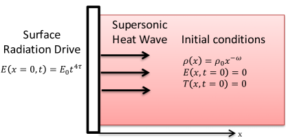
Figure 1: A description of the generalized non-equilibrium Marshak wave problem. A radiation temperature drive which obeys a temporal power law is applied at the surface ($x=0$) of a planar medium which is initially cold with zero radiation field and has an inhomogeneous material density which obeys a spatial power law. A nonlinear Marshak wave propagates into the medium and is conducted supersonically (with no material motion).

II Statement of the problem

Supersonic heat conduction by radiation is a common scenario in high energy density flows, in which radiative heat conduction dominates and hydrodynamic motion is negligible, and the material density remains constant in time. The non-equilibrium 1-group (gray) supersonic radiative transfer problem in planar slab symmetry for the radiation energy density $E\left(x,t\right)$ and the material energy density $u\left(x,t\right)$, is formulated by the following coupled equations (two-temperature approximation) [64, 65, 66, 67, 51, 68, 27]:

$$\frac{\partial E}{\partial t}+\frac{\partial F}{\partial x}=ck_{a}\left(U-E\right),$$ (1)

$$\frac{\partial u}{\partial t}=ck_{a}\left(E-U\right),$$ (2)

where $c$ is the speed of light, $k_{a}$ the radiation absorption macroscopic cross section (which is also referred to as the absorption coefficient or absorption opacity), and $U=aT^{4}$ with $T$ the material temperature and $a=\frac{8\pi^{5}k_{B}^{4}}{15h^{3}c^{3}}$ the radiation constant. The effective radiation temperature $T_{r}$ is related to the radiation energy density by $E=aT_{r}^{4}$. For optically thick media, the diffusion approximation of radiative transfer is applicable, and the radiation energy flux obeys Fick’s law:

$$F=-D\frac{\partial E}{\partial x},$$ (3)

where the radiation diffusion coefficient is given by:

$$D=\frac{c}{3k_{t}},$$ (4)

where $k_{t}=\rho\kappa_{R}$ is the total (absorption+scattering) macroscopic transport cross section, which we also refer to as the total opacity coefficient, where $\kappa_{R}$ the Rosseland mean opacity and $\rho$ is the (time independent) material mass density.

We now define a setup for a Marshak wave problem, which is also described schematically in Fig. 1. We assume a semi-infinite planar medium which is initially cold with no radiation field,

$$E\left(x,t=0\right)=U\left(x,t=0\right)=0,$$ (5)

with a (time independent) material mass density profile which is given by a spatial power law

$$\rho\left(x\right)=\rho_{0}x^{-\omega}.$$ (6)

We note that for a planar system to have a finite mass over a finite distance from the origin, we must require $\omega<1$. A Marshak wave is driven by imposing a surface radiation temperature at $x=0$, which obeys a temporal power law of the form:

$$T_{r}\left(x=0,t\right)\equiv T_{s}\left(t\right)=T_{0}t^{\tau},$$ (7)

so that the radiation energy density at the system left boundary is:

$$E\left(x=0,t\right)=E_{0}t^{4\tau},\ E_{0}=aT_{0}^{4}.$$ (8)

As was discussed in Ref. [27] (and in Refs. [69, 10, 5, 11, 28] for Marshak wave in thermodynamic equilibrium), this boundary condition of an imposed surface temperature is different than the common Marshak (or Milne) boundary condition, which represents the incoming flux from a heat bath. We will derive below in section III.4 a relation between the surface radiation temperature and the heat bath temperature, which will allow to define the same problem by a Marshak boundary condition with a prescribed bath temperature as a function of time.

We assume a power law temperature and density dependence of the total opacity

$$k_{t}\left(T,\rho\right)=\frac{1}{\mathcal{G}}T^{-\alpha}\rho^{1+\lambda},$$ (9)

the absorption opacity

$$k_{a}\left(T,\rho\right)=\frac{1}{\mathcal{G}^{\prime}}T^{-\alpha^{\prime}}\rho^{1+\lambda^{\prime}},$$ (10)

and the material energy density (energy per unit volume)

$$u\left(T,\rho\right)=\mathcal{F}T^{\beta}\rho^{1-\mu}.$$ (11)

This power law material model, which is characterized by the positive dimensional constants $\mathcal{G}$, $\mathcal{G}^{\prime}$, $\mathcal{F}$ and the non-negative exponents $\alpha,$ $\lambda,$ $\alpha^{\prime},$ $\lambda^{\prime},$ $\beta,$ and $\mu\leq 1$, serves as a good approximation for the properties of many materials and is commonly employed in the analysis of high energy density phenomena [35, 38, 39, 44, 42, 46, 23, 12, 27, 28]. Values of the exponents for several materials that were used in experiments of supersonic and subsonic Marshak waves are given in table 1, adopted from Refs. [5, 11, 70] (and references therein), for which photon scattering is negligible ($k_{t}=k_{a}$, so that $\alpha=\alpha^{\prime}$, $\lambda=\lambda^{\prime}$).

The problem defined by Eqs. (1)-(11) is a generalization of the problem defined in Ref. [27], where it was assumed that $\omega=0$ and $\beta=4$, to the more general case of an inhomogeneous density profile, $\omega\neq 0$, and realistic materials for which usually $\beta\neq 4$ (as evident from table 1).

Using the density profile (6) and the material model defined in Eqs. (9)-(11), Eqs. (1)-(2) are written in closed form as a set of nonlinear coupled partial differential equations for $E$ and $U$:

$$\frac{\partial E}{\partial t} =K\frac{\partial}{\partial x}\left(x^{\omega\left(1+\lambda\right)}U^{\frac{\alpha}{4}}\frac{\partial E}{\partial x}\right)$$ (12)

$$+Mx^{-\omega\left(1+\lambda^{\prime}\right)}U^{-\frac{\alpha^{\prime}}{4}}\left(U-E\right),$$

$$\frac{\partial U}{\partial t}=Px^{-\omega\left(\lambda^{\prime}+\mu\right)}U^{-\frac{\alpha^{\prime}}{4}}\left(E-U\right),$$ (13)

where we have defined the dimensional constants:

$$K=\frac{c\mathcal{G}}{3}\rho_{0}^{-1-\lambda}a^{-\frac{\alpha}{4}},$$ (14)

$$M=\frac{c}{\mathcal{G}^{\prime}}\rho_{0}^{1+\lambda^{\prime}}a^{\frac{\alpha^{\prime}}{4}},$$ (15)

$$P=\frac{4ca^{\frac{\alpha^{\prime}+\beta}{4}}\rho_{0}^{\lambda^{\prime}+\mu}}{\beta\mathcal{G}^{\prime}\mathcal{F}}.$$ (16)

III A Self-Similar solution

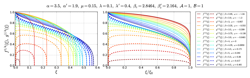
Figure 2: The radiation $f^{1/4}\left(\xi\right)$ (solid lines) and material $g^{1/4}\left(\xi\right)$ (dashed lines) temperature similarity profiles, for varying values of $\beta$, as listed in the legend (along with the resulting values of $\omega$). The parameters $\mathcal{A},\ \mathcal{B}$, the material exponents and the resulting $\beta_{c},\beta_{c}^{\prime}$ [Eqs. (34)-(35)], are listed in the title. The profiles are shown as a function of $\xi$ (left figure) and of $\xi/\xi_{0}$ (right figure), in order to display the variation of the profiles independently of the front coordinate $\xi_{0}$. Three types of solutions, as discussed in Sec. III.2, are evident: (i) for $\beta_{c}<\beta<4$, the density vanishes at the origin ($\omega<0$) and therefore, so does the material temperature, (ii) for $\beta=4$, the density is constant ($\omega=0$) and finite, which results in a material temperature that is finite at origin and lower than the radiation temperature and (iii) for $\beta>4$, the density diverges at the origin ($\omega>0$), so that the material and radiation temperatures are equal at the origin.

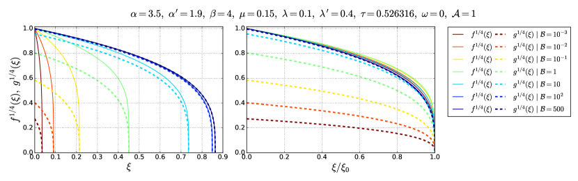
Figure 3: Same as Fig. 2, but for a material model with a fixed $\beta=4$ (as listed in the title), for $\mathcal{A}=1$ and varying values of $\mathcal{B}$ which are listed in the legend. The choice $\beta=4$ results in $\omega=0$ (a homogeneous density profile), which according to the analysis in Sec. III.2, results in a finite value of the material temperature at the origin. It is evident that the material and radiation temperature profiles become closer when $\mathcal{B}$ is increased, and that thermodynamic equilibrium limit $f^{1/4}\left(\xi\right)\approx g^{1/4}\left(\xi\right)$ is reached when $\mathcal{B}\gg 1$. As discussed in the text, it is also evident that $\xi_{0}$ increases with $\mathcal{B}$.

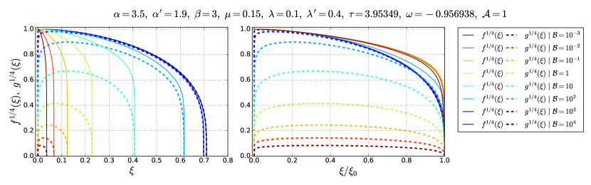
Figure 4: Same as Fig. 3, but for a choice of parameters for which $\omega<0$ (an increasing density profile). According to the analysis in Sec. III.2, this case results in $g\left(\xi\to 0\right)=0$, for any value of $\mathcal{B}$. It is evident as $\mathcal{B}\rightarrow\infty$, the material and radiation temperatures approach each other, while maintaining a zero material temperature at the origin, which results in increasingly larger slopes near the origin.

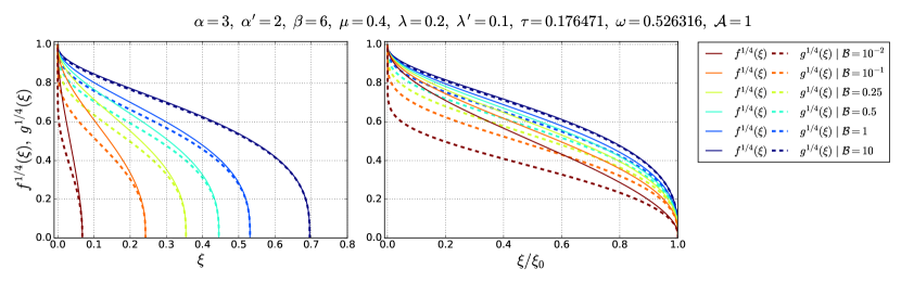
Figure 5: Same as Fig. 4, but for a choice of parameters for which $\omega>0$ (a decreasing density profile), that results in $g\left(\xi\to 0\right)=1$, which must hold for any value of $\mathcal{B}$. It is evident as $\mathcal{B}\rightarrow 0$, the material temperature becomes increasingly lower than the radiation temperature, while maintaining equilibrium at the origin, $g\left(\xi\to 0\right)=f\left(\xi\to 0\right)=1$. This results in increasingly steep negative slopes near the origin.

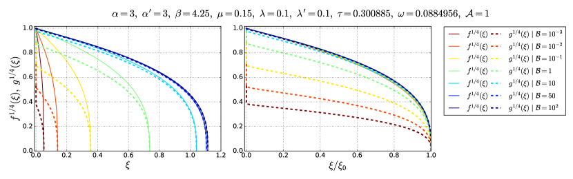
Figure 6: Same as Fig. 5, but for a choice of parameters with a smaller $\omega>0$, which results in an extremely sharp drop of the material temperature near the origin.

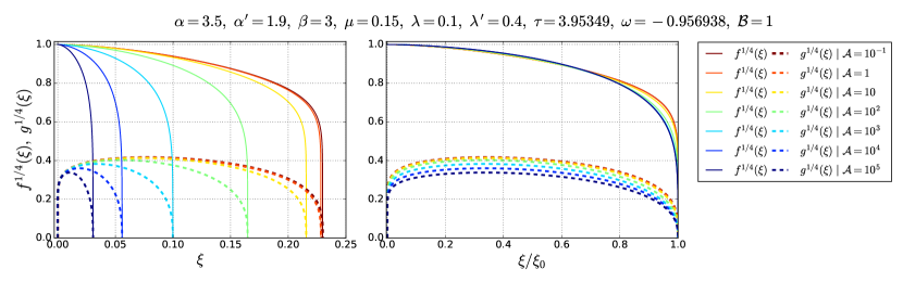
Figure 7: Same as Fig. 3, but for varying values of $\mathcal{A}$ (as listed in the legend) and a constant value $\mathcal{B}=1$. The choice of parameters is the same as in Fig. 4. It is evident that when $\mathcal{A}\lesssim 1$ it has a small effect on $\xi_{0}$ and the profile shapes. For larger values of $\mathcal{A}$, the value of $\xi_{0}$ and $g\left(\xi\right)$ decrease with respect to $\mathcal{A}$.

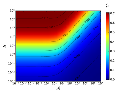
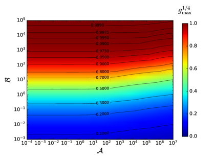
Figure 8: Color maps of the heat front coordinate $\xi_{0}$ (upper figure) and the maximal value of the material temperature profile $g_{\text{max}}^{1/4}=\underset{0\leq\xi\leq\xi_{0}}{\text{max}}\left[g^{1/4}\left(\xi\right)\right]$, as a function of $\mathcal{A}$ and $\mathcal{B}$. The material exponents are the same as in Figs. 4,7 (namely, $\alpha=3.9,\,\alpha^{\prime}=1.9,\,\beta=3,\,\mu=0.15,\,\lambda=0.1$ and $\lambda^{\prime}=0.4$, for which $\omega<0$). It is evident that $\xi_{0}$ and $g_{\text{max}}^{1/4}$ are increasing functions of $\mathcal{B}$ (in agreement with Fig. 4), and that thermodynamic equilibrium is reached for $\mathcal{B}\gg 1$ (as $g_{\text{max}}^{1/4}$ approaches unity). It is also evident that $\mathcal{A}$ has an effect on $\xi_{0}$ and $g_{\text{max}}^{1/4}$, only for large values $\mathcal{A}\apprge 10$, for which $\xi_{0}$ and $g_{\text{max}}^{1/4}$ are decreasing functions of $\mathcal{A}$ (in agreement with Fig. 7).

In Appendix A it is shown in detail, using the method of dimensional analysis [71, 32, 72, 42, 23], that the solution of the problem defined by the nonlinear gray diffusion model in Eqs. (12)-(13) with the initial and boundary conditions (5),(8), is self-similar, if and only if the surface temperature exponent and the spatial density exponent obey the following relations in terms of the various material exponents:

$$\tau =\frac{1-\mu}{\left(\beta-4\right)\left(1+\lambda^{\prime}\right)+\alpha^{\prime}\left(1-\mu\right)},$$ (17)

$$\omega =\frac{2\left(\beta-4\right)}{\left(\beta-4\right)\left(2+\lambda+\lambda^{\prime}\right)+\left(\alpha+\alpha^{\prime}\right)\left(1-\mu\right)}.$$ (18)

It is evident that $\omega=0$ if and only if $\beta=4$, in which case $\tau=\frac{1}{\alpha^{\prime}}$, in agreement with Ref. [27]. Conversely, $\beta\neq 4$ results in $\omega\neq 0$, and the problem has a self-similar solution only for an inhomogeneous density profile. As shown in Appendix A, when Eqs. (17)-(18) hold, the problem defines two dimensionless constants:

$$\mathcal{A} =E_{0}^{-\frac{\alpha+\alpha^{\prime}}{4\left(\alpha\tau+1\right)}}K^{\frac{\alpha^{\prime}\tau-1}{\alpha\tau+1}}M,$$ (19)

$$\mathcal{B} =E_{0}^{\frac{4-\beta-\alpha-\alpha^{\prime}}{4\left(\alpha\tau+1\right)}}K^{\frac{\left(\alpha^{\prime}+\beta-4\right)\tau-1}{\alpha\tau+1}}P,$$ (20)

and the Marshak wave problem has a self-similar solution which is expressed in terms dimensionless similarity profiles $f\left(\xi\right)$, $g\left(\xi\right)$ as:

$$E\left(x,t\right)=E_{0}t^{4\tau}f\left(\xi\right),$$ (21)

$$U\left(x,t\right)=E_{0}t^{4\tau}g\left(\xi\right),$$ (22)

where the dimensionless similarity coordinate is given by:

$$\xi=\frac{x}{t^{\delta}\left(KE_{0}^{\frac{\alpha}{4}}\right)^{\frac{1}{2-\omega\left(1+\lambda\right)}}},$$ (23)

and the similarity exponent is:

$$\delta=\frac{1+\alpha\tau}{2-\omega\left(\lambda+1\right)}=\frac{1}{2}\left(1+\frac{\alpha\left(1-\mu\right)+\left(\beta-4\right)\left(1+\lambda\right)}{\alpha^{\prime}\left(1-\mu\right)+\left(\beta-4\right)\left(1+\lambda^{\prime}\right)}\right).$$ (24)

The radiation and material temperature profiles are therefore given by

$$T_{r}\left(x,t\right)=T_{0}t^{\tau}f^{1/4}\left(\xi\right),$$ (25)

$$T\left(x,t\right)=T_{0}t^{\tau}g^{1/4}\left(\xi\right).$$ (26)

We see that when the absorption and total opacity have the same temperature and density dependence ($\alpha=\alpha^{\prime}$ and $\lambda=\lambda^{\prime}$ or $\alpha=\alpha^{\prime}$ and $\beta=4$), we acquire $\delta=1$, in agreement with Ref. [27]. As shown in Appendix A, by plugging the self-similar representation (21)-(22) into the gray diffusion system (12)-(13), all dimensional quantities are factored out, and the following (dimensionless) second order ordinary differential equations (ODE) system for the similarity profiles is obtained:

$$4\tau f\left(\xi\right)-\delta\xi f^{\prime}\left(\xi\right)=\xi^{\omega\left(1+\lambda\right)}\Bigg{(}\frac{1}{\xi}\omega\left(\lambda+1\right)g^{\frac{\alpha}{4}}\left(\xi\right)f^{\prime}\left(\xi\right)$$

$$+g^{\frac{\alpha}{4}-1}\left(\xi\right)\left[\frac{\alpha}{4}f^{\prime}\left(\xi\right)g^{\prime}\left(\xi\right)+g\left(\xi\right)f^{\prime\prime}\left(\xi\right)\right]\Bigg{)}$$

$$-\mathcal{A}\xi^{-\omega\left(1+\lambda^{\prime}\right)}g^{-\frac{\alpha^{\prime}}{4}}\left(\xi\right)\left(f\left(\xi\right)-g\left(\xi\right)\right),$$ (27)

$$4\tau g\left(\xi\right)-\delta\xi g^{\prime}\left(\xi\right)=\mathcal{B}\xi^{-\omega\left(\lambda^{\prime}+\mu\right)}g^{1-\frac{\alpha^{\prime}+\beta}{4}}\left(\xi\right)\left(f\left(\xi\right)-g\left(\xi\right)\right).$$ (28)

The surface radiation temperature boundary condition [Eq. (8)], is written in terms of the radiation energy similarity profile as:

$$f\left(0\right)=1.$$ (29)

It is evident that the dimensionless problem defined by Eqs. (27)-(29) depends only on the material exponents $\alpha,\alpha^{\prime},\lambda,\lambda^{\prime},\beta,\mu$ and the dimensionless constants $\mathcal{A},\mathcal{B}$. We also see that if $\beta=4$ we get $\mathcal{B}=\epsilon\mathcal{A}$ where $\epsilon=\frac{a}{\mathcal{F}}$, and the dimensionless problem is reduced to the homogeneous solution given in Ref. [27].

Nonlinear conduction is characterized by a steep heat front, that is, there exists a finite heat front coordinate, $\xi_{0}$, such that $f\left(\xi\right)=g\left(\xi\right)=0$ for $\xi\geq\xi_{0}$. According to Eq. (23), the heat front propagates in time according to a temporal power law:

$$x_{F}\left(t\right)=\xi_{0}t^{\delta}\left(KE_{0}^{\frac{\alpha}{4}}\right)^{\frac{1}{2-\omega\left(1+\lambda\right)}}.$$ (30)

As shown in many works on nonlinear Marshak waves in thermodynamic equilibrium, for which $T_{r}\equiv T$ [30, 31, 73, 66, 74, 41, 42, 39, 27, 28] and more recently in non-equilibrium as well [27], it is customary to calculate the value of $\xi_{0}$ via iterations of a “shooting method”. This is done by integrating Eqs. (27)-(28) starting from a trial value of $\xi_{0}$ towards the origin, $\xi=0$, resulting in a numerical value for $f\left(0\right)$. The trial $\xi_{0}$ is adjusted until the surface radiation temperature boundary condition, $f\left(0\right)=1$, is satisfied. To the best of our knowledge, analytical solutions to Eqs. (27)-(28) exist only when $\beta=4$ ($\omega=0$) and $\alpha=\alpha^{\prime}$, as was found in Ref. [27], otherwise, the similarity profiles and $\xi_{0}$ must be obtained numerically. Numerical results for the similarity profiles are shown in Figs. 2-7, which display the different characteristics of the solutions for cases with $\omega=0$, $\omega>0$ and $\omega<0$, as well as the behavior of the solutions for varying values of $\mathcal{A}$ and $\mathcal{B}$. These characteristics of the solutions are discussed in detail below in Sec. III.2.

III.1 Range of validity

The similarity solution is invalid when $\omega\geq 1$ (in which case there is an infinite mass over any finite distance from the origin), or when $\delta\leq 0$ (the wave does not propagate outwards). In order to further analyze the solution’s properties and range of validity, we first consider the case with $\mu<1$, for which it is customary to write $\tau$, $\omega$ and $\delta$ [Eqs. (17)-(18), (24)], as functions of $\beta$:

$$\tau\left(\beta\right)=\left(\frac{1-\mu}{1+\lambda^{\prime}}\right)\frac{1}{\beta-\beta_{c}},$$ (31)

$$\omega\left(\beta\right) =\left(\frac{1}{1+\overline{\lambda}}\right)\frac{\beta-4}{\beta-\beta_{c}^{\prime}},$$ (32)

$$\delta\left(\beta\right)=\left(\frac{1+\overline{\lambda}}{1+\lambda^{\prime}}\right)\frac{\beta-\beta_{c}^{\prime}}{\beta-\beta_{c}},$$ (33)

where we have defined two critical values of $\beta$:

$$\beta_{c}=4-\frac{\alpha^{\prime}\left(1-\mu\right)}{1+\lambda^{\prime}},$$ (34)

$$\beta_{c}^{\prime}=4-\frac{\overline{\alpha}\left(1-\mu\right)}{1+\overline{\lambda}}.$$ (35)

and the average opacity temperature and density exponents:

$$\overline{\alpha}=\frac{1}{2}\left(\alpha+\alpha^{\prime}\right),\ \ \overline{\lambda}=\frac{1}{2}\left(\lambda+\lambda^{\prime}\right).$$ (36)

We see that $\tau$ diverges at $\beta=\beta_{c}<4$ while $\omega$ diverges at $\beta=\beta_{c}^{\prime}<4$. We also see that $\tau<0$ for $\beta<\beta_{c}$, $\tau>0$ for $\beta>\beta_{c}$ and there is no solution with $\tau=0$. These cases correspond, respectively, to a decreasing, increasing and constant temperature drive [see Eq. (7)]. Similarly, $\omega<0$ for $\beta_{c}^{\prime}<\beta<4,$ while $\omega=0$ for $\beta=4$ and $\omega>0$ otherwise; cases which correspond, respectively, to an increasing, constant and decreasing spatial density profiles [see Eq. (6)]. In addition, $\omega<\frac{1}{1+\overline{\lambda}}<1$ for $\beta>\beta_{c}^{\prime}$. We also see that $\delta<0$ for $\text{$\min\left(\beta_{c},\beta_{c}^{\prime}\right)$}<\beta<\text{max}\left(\beta_{c},\beta_{c}^{\prime}\right)$. As a result, solutions with $\tau<0$ exist only for $\omega>0$, while on the other hand, solutions with $\tau>0$ exist for negative, positive and zero $\omega$. In addition, for $0\leq\beta<\min\left(\beta_{c},\beta_{c}^{\prime}\right)$, for which $\omega>0$ and $\tau<0$, the solution is valid provided that $\omega<1$ as well. In summary, the solution is always invalid for $\text{$\min\left(\beta_{c},\beta_{c}^{\prime}\right)$}\leq\beta\leq\text{max}\left(\beta_{c},\beta_{c}^{\prime}\right)$ and also for values of $\beta$ in the range $0\leq\beta<\min\left(\beta_{c},\beta_{c}^{\prime}\right)$ for which $\omega\left(\beta\right)>1$.

To illustrate these properties, we first analyze the more simple case in which the total and absorption opacities have the same temperature and density dependence, that is, when $\alpha=\alpha^{\prime}$ and $\lambda=\lambda^{\prime}$. In that case $\tau$ and $\omega$ diverge at the same value of $\beta=\beta_{c}=\beta_{c}^{\prime}$, while $\delta\equiv 1$ and is independent of $\beta$. In Fig. 9 the resulting $\tau\left(\beta\right)$ and $\omega\left(\beta\right)$ are plotted as a function of $\beta$, for several material models (assuming $\alpha=\alpha^{\prime}$, $\lambda=\lambda^{\prime}$). In all of those cases it turns out that $\omega>1$ for $\beta<\beta_{c}$, so that the similarity solution is invalid for $\beta\leq\beta_{c}$. Conversely, since $\underset{\beta\rightarrow\infty}{\lim}\omega\rightarrow\frac{1}{1+\lambda}<1$, the solution is valid for any $\beta>\beta_{c}$. It also happens that for each of the chosen materials (given in Table 1), $\beta_{c}$ is larger than the value of the material’s $\beta$, and therefore, there are no self-similar solutions for these given materials. In addition, since $\tau>0$ if and only if $\beta>\beta_{c}$, the similarity solutions exist in those cases only for a strictly increasing radiation temperature drive ($\tau>0$). In Fig. 10 we show similar plots for $\tau\left(\beta\right)$, $\omega\left(\beta\right)$ and $\delta\left(\beta\right)$ for more general cases of $\alpha,\alpha^{\prime},\lambda,\lambda^{\prime},\mu$, with $\alpha\neq\alpha^{\prime}$ or $\lambda\neq\lambda^{\prime}$. Various different characteristics are evident. Some cases have valid solutions only for $\beta>\beta_{c}$ or $\beta>\beta_{c}^{\prime}$ for which $\tau\left(\beta\right)>0$. Other cases have valid solutions in a range $0\leq\beta<\beta^{*}<\text{min$\left(\beta_{c},\beta_{c}^{\prime}\right)$}$ for which $\tau\left(\beta\right)<0$. Interestingly, some cases have $\beta_{c},\beta_{c}^{\prime}<0$, so that the solutions are valid for any $\beta$, and have $\tau\left(\beta\right)>0$. It is also evident that there exists solutions with $0<\delta<1$ (decelerating heat front) as well as $\delta>1$ (accelerating heat front).

Finally, for $\mu=1$ (a density independent material energy density) and $\beta\neq 4$, Eqs. (17)-(18), (24) give the following $\beta$ independent exponents:

$$\tau =0,$$ (37)

$$\omega=\frac{1}{1+\overline{\lambda}},$$ (38)

$$\delta=\frac{1+\overline{\lambda}}{1+\lambda^{\prime}}.$$ (39)

In summary, it was shown that depending on the material exponents, $\alpha,\alpha^{\prime},\lambda,\lambda^{\prime},\beta,\mu$, the generalized solutions, when they are valid, can have a temporally increasing ($\tau>0$), decreasing ($\tau<0$) and constant ($\tau=0$) surface temperature drive.

Material	$\alpha$	$\beta$	$\lambda$	$\mu$
$\mathrm{Au}$	$1.5$	$1.6$	$0.2$	$0.14$
$\mathrm{Al}$	$3.1$	$1.2$	$0.368$	$0$
$\mathrm{SiO_{2}}$	$2$	$1.23$	$0.61$	$0.1$
$\mathrm{Ta_{2}O_{5}}$	$1.78$	$1.37$	$0.24$	$0.12$
$\mathrm{C_{15}H_{20}O_{6}}$	$5.29$	$0.94$	$0.95$	$0.038$
Ideal Gas	$3.5$	$1$	$1$	$0$

Table 1: Values of material temperature and density exponents $\alpha,\beta,\lambda,\mu$ for various materials (adopted from Refs. [5, 11, 70] and references therein). In the last row, the values are listed for a material with an ideal gas equation of state a pure free-free absorption opacity.

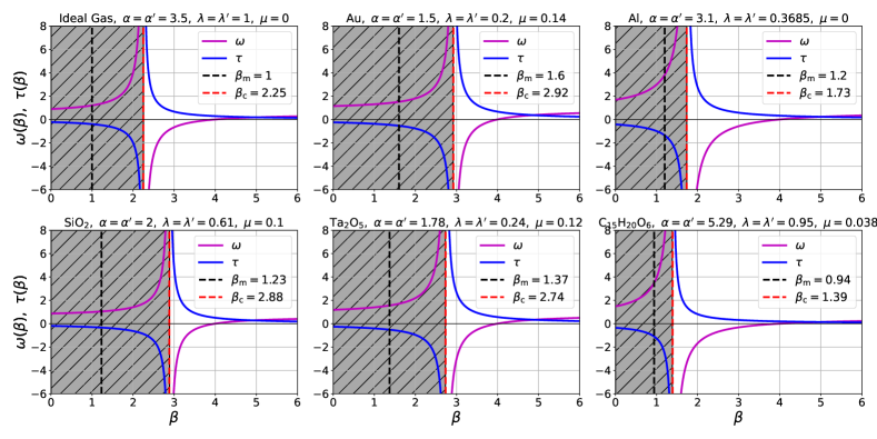
Figure 9: The temperature drive exponent $\tau$ (blue) and spatial density exponent $\omega$ (magenta), for which the solution of the Marshak wave problem is self-similar [Eqs. (17)-(18) or (31)-(32)], as a function of the material energy density power $\beta$. The results are shown for $\alpha=\alpha^{\prime}$, $\lambda=\lambda^{\prime}$ using the parameters $\alpha,\lambda,\mu$ of various materials (given in Table 1). Vertical lines are shown for the critical value $\beta=\beta_{c}=\beta_{c}^{\prime}$ [Eqs. (34)-(35)], and $\beta=\beta_{m}$, the actual temperature exponent of each material (see Table 1). It is evident that $\omega>1$ for $\beta<\beta_{c}$, which means that similarity solutions do not exist for $\beta<\beta_{c}$ (marked area). Since for all materials shown, $\beta_{c}>\beta_{m}$, the solution is not self-similar for $\beta=\beta_{m}$. It is also evident that $\tau>0$ for $\beta>\beta_{c}$ and $\tau<0$ for $\beta<\beta_{c}$, which means that similarity solutions must have an increasing temperature drive ($\tau>0$). Finally, for the shown materials $\beta_{c}<4$, and since $\omega$ changes sign at $\beta=4$, self-similar solutions exist for both increasing ($\omega<0$) and decreasing ($\omega>0$) spatial density profiles.

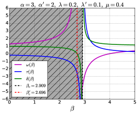
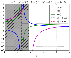
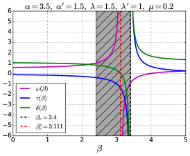
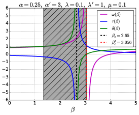
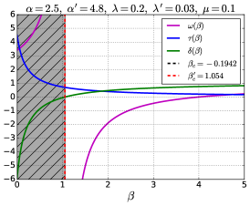
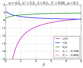
Figure 10: Similar plot to Fig. 9, but for cases for which $\alpha\neq\alpha^{\prime}$ or $\lambda\neq\lambda^{\prime}$. The similarity exponent $\delta\left(\beta\right)$ [Eq. (24) or (33)] is also plotted. Vertical lines are shown for the critical values $\beta=\beta_{c}$ [Eq. 34] and $\beta=\beta_{c}^{\prime}$ [Eq. 35], with the values listed in the legend. The range of $\beta$ for which the self-similar solution is invalid (marked in gray), is where $\delta\left(\beta\right)\leq 0$ or $\omega\left(\beta\right)\geq 1$, as discussed in the text. Six different cases are shown, with different characteristics and ranges of validity.

III.2 The solution near the origin

The behavior of the solution near the system’s boundary, can be analyzed without having to solve the full coupled ODE system (27)-(28). We expand the solution to first order near $\xi\rightarrow 0$:

$$f\left(\xi\right) \approx 1+f^{\prime}\left(0\right)\xi+O\left(\xi^{2}\right),$$ (40)

$$g\left(\xi\right) \approx g_{0}+g^{\prime}\left(0\right)\xi+O\left(\xi^{2}\right).$$ (41)

where $g_{0}=g\left(\xi=0\right)$. By substituting the expansion (40)-(41) into the matter equation (28) and keeping the zero order terms, we find:

$$\begin{cases}g_{0}=1&\omega>0\\ g_{0}\left(1+\frac{4\tau}{\mathcal{B}}g_{0}^{\frac{\alpha^{\prime}+\beta-4}{4}}\right)=1&\omega=0\\ g_{0}=0&\omega<0\end{cases}$$ (42)

These three qualitatively different forms of the solution near the origin are displayed in Figs. 2-7. For $\omega=0$ (so that $\beta=4$ and $\tau=1/\alpha^{\prime}$), $g_{0}$ obeys a nonlinear equation, as was found in Ref. [27], whose solution may attain, as a function of $\mathcal{B}$ and $\alpha^{\prime}$, any value in the range $0<g_{0}<1$, that is, the dimensionless material temperature at the origin is finite and can vary continuously between 0 (highly non-LTE) and 1 (the LTE limit), as shown in Fig. 3. On the other hand, we see that for $\omega>0$ (that is, $\beta>4$), $g_{0}=f\left(0\right)=1$, that is, the material and radiation are always in equilibrium at the origin. This is a result of the density $\rho\propto x^{-\omega}$ diverging at the origin, leading to a divergent absorption coefficient $k_{a}\propto\rho^{\lambda^{\prime}+1}\propto x^{-\omega\left(\lambda^{\prime}+1\right)}$, which results in an infinitely strong coupling and an immediate equilibration at $\xi\rightarrow 0$, as shown in Figs. 2, 5 and 6. Conversely, when $\omega<0$ (that is, $\beta<4$), the density and consequently the absorption coefficient vanish at the origin, which leads to no coupling between the radiation and material, which results in a cold material at $\xi\rightarrow 0$, so that $g_{0}=0$. This results in a material temperature profile which is not monotonic, as shown in Figs. 4 and 7. These three types of solutions are shown in Fig. 3, where the temperature profiles are displayed for a varying value of $\beta$.

III.3 The thermodynamic equilibrium limit

Using Eqs. (13) and (20), it can be inferred that the dimensionless constant parameter $\mathcal{B}$ quantifies the material coupling to the radiation field by the emission absorption process, since:

$$\frac{\partial U}{\partial t}\propto\mathcal{B}x^{-\omega\left(\lambda^{\prime}+\mu\right)}U^{-\frac{\alpha^{\prime}}{4}}\left(E-U\right),$$ (43)

which shows that the $\mathcal{B}$ determines the equilibration rate. Equivalently, Eq. (28) shows that when $\mathcal{B}\gg 1$ we have $g\left(\xi\right)\approx f\left(\xi\right)$, that is, the material and radiation temperature profiles approach a common form, that is, a state of thermodynamic equilibrium is reached locally. This fact is demonstrated in Figs. 3-6, where it is evident that as $\mathcal{B}$ increases, $g^{1/4}\left(\xi\right)$ and $f^{1/4}\left(\xi\right)$ converge to the same profile. As discussed in the previous section, when $\omega<0$, the material temperature must vanish at the origin for any value of $\mathcal{A}$ and $\mathcal{B}$. However, since $f\left(0\right)=1$, when $\mathcal{B}\rightarrow\infty$ the thermodynamic equilibrium limit must be reached, which results in a very sharp increase of $g\left(\xi\right)$ near the origin from 0 to 1, as shown in Fig. 4. Conversely, when $\omega>0$, we must have $g_{0}=1$, as equilibrium is always reached at the origin, independently of the values of $\mathcal{A}$ and $\mathcal{B}$. However, for $\mathcal{B}\lesssim 1$ a significant state of non-equilibrium occurs for $\xi>0$, which results in a sharp decrease of $g\left(\xi\right)$ near the origin from a value of 1 to a lower finite value, as shown in Figs. 5-6.

In Fig. 8 the heat front coordinate $\xi_{0}$ and the maximal value of the dimensionless material temperature, $g_{\text{max}}^{1/4}=\underset{0\leq\xi\leq\xi_{0}}{\text{max}}\left[g^{1/4}\left(\xi\right)\right]$, are shown as functions of $\mathcal{A}$ and $\mathcal{B}$, for a case with $\omega<0$. From the discussion above, when the equilibrium limit is reached, the value of $g_{\text{max}}^{1/4}$ should reach unity, for any value of $\omega$. It is evident from Fig. 8 that $g_{\text{max}}^{1/4}$ depends weakly on $\mathcal{A}$, and approaches unity as the value of $\mathcal{B}$ increases.

Finally, it is evident from Figs. 3-6, as well as from Fig. 8, that the front coordinate $\xi_{0}$ is an increasing function of $\mathcal{B}$. This can be expected, since larger values of $\mathcal{B}$ give rise to a larger coupling between the radiation and material, leading to a higher material temperature, which results in a smaller total opacity [see Eq. 9], that leads to a faster heat propagation. Figs. 7 and 8 show that for moderate values $\mathcal{A}\lesssim 1$, $\xi_{0}$ and the profile shapes depends very weakly on $\mathcal{A}$. For larger values of $\mathcal{A}$, the material temperature profiles $g^{1/4}\left(\xi\right)$ decrease with respect to $\mathcal{A}$, resulting in a smaller values of $\xi_{0}$.

III.4 Marshak boundary condition

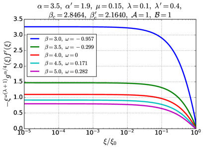
Figure 11: The flux similarity profile [see Eq. 47], for various values of $\omega$ (as listen in the legend), and for a choice of parameters which is listed in the title (same as in Fig. 2).

Non-equilibrium Marshak waves [47, 48, 27], as well as many other non-equilibrium heat wave benchmarks [75, 76, 77, 78, 79, 80, 81, 82, 83, 84, 85, 86, 87, 88], are specified in terms of a given incoming radiative flux, rather than a temperature boundary condition (as in Eq. (8)). The latter boundary condition applies more naturally in the diffusion approximation, while the former is more natural to use in the solution of the radiation transport equation, which has the angular surface flux as a boundary condition (as will be discussed below in section IV.1). Nevertheless, these two different boundary conditions can be related [69, 10, 5, 11, 27, 28].

The incoming flux boundary condition, which is known as the Marshak boundary condition [47, 48, 69, 27] is given by:

$$\frac{4}{c}F_{\text{inc}}\left(t\right)=E\left(x=0,t\right)+\frac{2}{c}F\left(x=0,t\right),$$ (44)

where $F_{\text{inc}}\left(t\right)$ is the incoming flux at $x=0$. The incoming flux to a medium which is coupled to a heat bath at temperature $T_{\text{bath}}\left(t\right)$, is given by $F_{\text{inc}}\left(t\right)=\frac{ac}{4}T_{\text{bath}}^{4}\left(t\right)$. The Marshak boundary condition (44) results from the diffusion limit of the exact Milne boundary condition of radiation transport (see section IV.1 below). Using the surface radiation temperature, $E\left(x=0,t\right)=aT_{s}^{4}\left(t\right)$, in the Marshak boundary condition (44) gives:

$$T_{\text{bath}}\left(t\right)=\left(T_{s}^{4}\left(t\right)+\frac{2}{ac}F\left(x=0,t\right)\right)^{\frac{1}{4}},$$ (45)

which is a relation between the bath temperature, the surface radiation temperature and the net surface flux. By using Eqs. (3)-(4), the radiation flux can be written in a self-similar form:

$$F\left(x,t\right) =K^{\frac{1}{2-\omega\left(1+\lambda\right)}}E_{0}^{1+\frac{\alpha}{4\left(2-\omega\left(1+\lambda\right)\right)}}t^{4\tau+\delta-1}\mathcal{S}\left(\xi\right),$$ (46)

where the (dimensionless) similarity flux profile is given by:

$$\mathcal{S}\left(\xi\right)=-\xi^{\omega\left(1+\lambda\right)}g^{\frac{\alpha}{4}}\left(\xi\right)f^{\prime}\left(\xi\right).$$ (47)

The radiation surface temperature is given by Eq. (7), so that the bath temperature, according to Eq. (45), can be written explicitly as a function of time:

$$T_{\text{bath}}\left(t\right)=\left(1+Bt^{\delta-1}\right)^{\frac{1}{4}}T_{0}t^{\tau},$$ (48)

where we have defined the bath coefficient:

$$B =\frac{2}{c}\left(\frac{c\mathcal{G}}{3}\rho_{0}^{-1-\lambda}T_{0}^{\alpha}\right)^{\frac{1}{2-\omega\left(1+\lambda\right)}}\mathcal{S}\left(0\right),$$ (49)

where the dimensionless radiation flux at the origin is:

$$\mathcal{S}\left(0\right)=-\lim_{\xi\to 0}\xi^{\omega\left(1+\lambda\right)}g^{\frac{\alpha}{4}}\left(\xi\right)f^{\prime}\left(\xi\right).$$ (50)

We note that $\mathcal{S}\left(0\right)$ does not diverge for both cases of diverging and vanishing density at the origin. This is demonstrated in Fig. 11, where $\mathcal{S}\left(\xi\right)$ is displayed for various values of $\omega$. We also note that Eq. (48) shows that only for $\delta=1$ the bath temperature is given by a temporal power law, which has the same temporal power $\tau$ of the surface temperature (in agreement with Ref. [27]). Finally, we note that since $B\propto\mathcal{G}^{\frac{1}{2-\omega\left(\lambda+1\right)}}$, when the total opacity increases, the bath temperature $T_{\text{bath}}\left(t\right)$ becomes closer to the surface temperature $T_{s}\left(t\right)$.

IV Comparison with simulations

IV.1 Transport setup

We now construct a setup for gray transport calculations of the gray diffusion problem defined in Sec. II. The one dimensional, one group (gray) transport equation for the radiation intensity field $I\left(x,\mu,t\right)$ in slab symmetry is [89, 77, 65, 81, 73, 66, 27]

$$\left(\frac{1}{c}\frac{\partial}{\partial t}+\mu\frac{\partial}{\partial x}\right)I\left(x,\mu,t\right)+ \left(k_{a}+k_{s}\right)I\left(x,\mu,t\right)$$

$$=\frac{ac}{4\pi}k_{a}T^{4}\left(x,t\right)+\frac{1}{2}k_{s} \int_{-1}^{1}d\mu^{\prime}I\left(x,\mu^{\prime},t\right),$$ (51)

where $\mu$ is the directional angle cosine, $k_{a}=k_{a}\left(T,\rho\right)$ and $k_{s}=k_{s}\left(T,\rho\right)$, are, respectively, the absorption and elastic scattering macroscopic cross sections, which are functions of the local material temperature and density. The radiation field is coupled to the material via the material energy equation:

$$\frac{\partial u\left(T,\rho\right)}{\partial t} =k_{a}\left[2\pi\int_{-1}^{1}d\mu^{\prime}I\left(x,\mu^{\prime},t\right)-acT^{4}\left(x,t\right)\right].$$ (52)

where $u\left(T,\rho\right)$ is the material energy density. The radiation energy density is given by:

$$E\left(x,t\right)=\frac{2\pi}{c}\int_{-1}^{1}d\mu^{\prime}I\left(x,\mu^{\prime},t\right),$$ (53)

and the radiation temperature is $T_{r}\left(x,t\right)=\left(E\left(x,t\right)/a\right)^{1/4}$. The diffusion limit holds for optically thick problems. In that case, the transport problem (51)-(52) can be approximated by the gray diffusion problem defined by equations (1)-(3), with the total opacity $k_{t}=k_{s}+k_{a}$. Therefore, a transport setup of the diffusion problem defined in Sec. II should have the following effective elastic scattering opacity:

$$k_{s}\left(T,\rho\right) =k_{t}\left(T,\rho\right)-k_{a}\left(T,\rho\right)$$

$$=\frac{1}{\mathcal{G}}T^{-\alpha}\rho^{1+\lambda}-\frac{1}{\mathcal{G}^{\prime}}T^{-\alpha^{\prime}}\rho^{1+\lambda^{\prime}}.$$ (54)

We note that unless $\alpha=\alpha^{\prime}$ and $\lambda=\lambda^{\prime}$, this form the scattering opacity is not a good model for real materials, but is used here to construct a gray transport problem which is mathematically equivalent, in the optically thick limit, to a gray diffusion problem whose total and absorption opacities are power laws with respect to temperature and density. Moreover, since the scattering opacity must be positive, the gray transport problem is well defined only if $k_{t}\left(T,\rho\right)\geq k_{a}\left(T,\rho\right)$, which must hold for the relevant temperatures and densities in the problem. This constraint does not have to hold for the gray diffusion problem, which is well defined for any functions $k_{t}$, $k_{a}$. We note that due to the complex nature of opacity spectra of mid or high-Z hot dense plasmas, the total (Rosseland) opacity can be lower than the absorption (Planck) opacity [65, 66, 73, 90, 91], in which case an equivalent gray transport problem cannot be defined.

The boundary condition for the transport problem is defined via the incident radiation field at $x=0$ for incoming directions $\mu>0$, of a a black body radiation bath

$$I\left(x=0,\mu,t\right)=\frac{ac}{4\pi}T_{\text{bath}}^{4}\left(t\right),$$ (55)

where the time dependent bath temperature drive is taken from the Marshak (Milne) boundary condition using the radiation temperature and flux which are taken from the gray diffusion solution [Eq. (48)], as detailed in Sec. III.4. The Marshak boundary condition [Eq. (44)] is derived by the diffusion limit approximation of the exact transport boundary condition given by Eq. (55).

Since the diffusion limit is applicable for optically thick problems, we expect gray transport results to have a good agreement with diffusion simulations and the self-similar solutions in this limit. Nevertheless, for optically thick problems with low absorption but high photon scattering ($k_{a}\ll k_{t}$), such that $\mathcal{B}\lesssim 1$, we expect transport results to agree well with diffusion, while the radiation and material are significantly out of equilibrium. Several examples of this scenario will be shown below.

IV.2 Test cases

Based on the self-similar solutions, we define six benchmarks for which we specify in detail the setups for gray diffusion and transport computer simulations. We conducted gray diffusion simulations and stochastic implicit Monte-Carlo (IMC) [75, 92, 93, 94, 95, 96, 97] and deterministic discrete-ordinates ($S_{N}$) transport simulations. The diffusion simulations were performed without the application of flux limiters. The $S_{N}$ simulations were performed using a numerical method that is detailed in Ref. [98], while the IMC simulations employed the novel numerical scheme that is described in Refs. [99, 81, 82].

All cases are run until the final time $t=1\text{ns}$, and the radiation surface temperature drive is increased to a final temperature of $1\text{keV}$:

$$T_{s}\left(t\right)=\left(\frac{t}{\text{ns}}\right)^{\tau}\ \text{keV},$$ (56)

so that $T_{0}=\text{keV}/\text{ns}^{\tau}$ for all cases. In addition, we take in all cases a spatial density profile:

$$\rho\left(x\right)=\left(\frac{x}{\text{cm}}\right)^{-\omega}\ \text{g}/\text{cm}^{3}.$$ (57)

so that $\rho_{0}=1\text{g}\cdot\text{cm}^{\omega-3}$. The temperature profiles are plotted at the final time and also at the times when the heat front reaches $20\%$ and $60\%$ of the final front position.

In tests 1 and 2 we define a material model with $\beta<4$, so that $\omega<0$ and that the material temperature is zero at the origin, increases until reaching a maximum and then decreases again towards the front. In cases 3-5 the material models have $\beta>4$ so that $\omega>0$, and the radiation and material temperatures are equal at the origin. Tests 1-4 have $\mathcal{B}\lesssim 1$ so that a significant deviation from equilibrium occurs. Test 5 has $\mathcal{B}\gg 1$ which results in the thermodynamic equilibrium limit, for which the radiation and material temperatures are very close throughout the heat wave. Finally, Test 6, which also has $\mathcal{B}\gg 1$, but since the density is extremely small in a wide range near the origin, a state of equilibrium is not reached in that region.

All cases were defined such that the total optical depth is large, so that the diffusion limit is applicable, and transport simulations results should agree with the gray diffusion self-similar solutions and simulations.

Since exact closed form analytical solutions of Eqs. (27)-(28) for the temperature profiles do no exist, tabulated exact numerical solution profiles for all cases are given in table 2. In addition, we give simple and closed form but approximate fitted analytic profiles in table 3, which are accurate to about $0.5\%$.

	Test 1		Test 2		Test 3		Test 4		Test 5		Test 6
$\xi_{0}$	$1.274605$		$0.615503$		$0.314115$		$0.484638$		$0.530730$		$1.198678$
$\xi/\xi_{0}$	$f^{1/4}\left(\xi\right)$	$g^{1/4}\left(\xi\right)$	$f^{1/4}\left(\xi\right)$	$g^{1/4}\left(\xi\right)$	$f^{1/4}\left(\xi\right)$	$g^{1/4}\left(\xi\right)$	$f^{1/4}\left(\xi\right)$	$g^{1/4}\left(\xi\right)$	$f^{1/4}\left(\xi\right)$	$g^{1/4}\left(\xi\right)$	$f^{1/4}\left(\xi\right)$	$g^{1/4}\left(\xi\right)$
0	1	0	1	0	1	1	1	1	1	1	1	0
$10^{-6}$	1	0.3463	1	0.010182	0.99987	0.97389	0.99795	0.98549	0.99968	0.99951	1	0.0025247
$10^{-5}$	1	0.40853	1	0.019658	0.99959	0.95101	0.9955	0.97292	0.99899	0.99872	1	0.0079838
0.0001	1	0.48063	1	0.037954	0.99868	0.91732	0.99012	0.95124	0.9968	0.99637	1	0.025247
0.0005	1	0.53693	1	0.060113	0.99692	0.88791	0.98262	0.92829	0.9928	0.99221	1	0.056454
0.001	1	0.56257	1	0.073278	0.99553	0.87386	0.97769	0.91585	0.98977	0.98909	1	0.079837
0.005	0.99999	0.62477	1	0.11605	0.98909	0.83765	0.9593	0.87914	0.97658	0.97567	1	0.17848
0.01	0.99995	0.65239	1	0.14146	0.98378	0.82	0.94659	0.85883	0.9663	0.96526	1	0.25225
0.05	0.99837	0.71601	0.99998	0.22394	0.95741	0.76988	0.89478	0.79375	0.91888	0.91757	1	0.55298
0.1	0.99298	0.73924	0.99983	0.27272	0.93334	0.74045	0.85459	0.75214	0.87876	0.87737	1	0.74168
0.15	0.98375	0.74747	0.99931	0.30574	0.91201	0.71883	0.8218	0.72084	0.84492	0.84351	1	0.84704
0.2	0.97077	0.74769	0.99815	0.33111	0.89177	0.70038	0.79232	0.69399	0.81402	0.81262	0.99998	0.90706
0.25	0.95413	0.74215	0.9961	0.35158	0.87192	0.68356	0.76462	0.66952	0.78473	0.78336	0.99992	0.94156
0.3	0.93389	0.73185	0.99286	0.36838	0.85207	0.66761	0.73788	0.64642	0.75633	0.755	0.99977	0.96171
0.35	0.91009	0.71732	0.98818	0.38214	0.83193	0.65208	0.71159	0.62408	0.72837	0.72709	0.9994	0.97363
0.4	0.88273	0.69885	0.98178	0.39317	0.81128	0.63665	0.68537	0.60208	0.70049	0.69926	0.99862	0.98055
0.45	0.85176	0.67658	0.97339	0.4016	0.78988	0.62109	0.65893	0.5801	0.6724	0.67123	0.99713	0.98406
0.5	0.81706	0.65054	0.96271	0.40745	0.76751	0.60515	0.63196	0.55784	0.64383	0.64274	0.99452	0.9848
0.55	0.77847	0.62067	0.94943	0.41063	0.7439	0.58862	0.60419	0.53503	0.61451	0.61348	0.9902	0.9828
0.6	0.73573	0.58681	0.93315	0.41097	0.71871	0.57122	0.57528	0.51135	0.5841	0.58315	0.9834	0.97764
0.65	0.68847	0.54869	0.9134	0.40817	0.69153	0.55264	0.54484	0.48644	0.55223	0.55136	0.9731	0.96855
0.7	0.63614	0.50588	0.88956	0.40178	0.66178	0.53243	0.51236	0.45982	0.51839	0.5176	0.95799	0.95434
0.75	0.57793	0.45773	0.86074	0.39109	0.62862	0.50997	0.4771	0.43082	0.48185	0.48116	0.93621	0.93324
0.8	0.51255	0.4032	0.82555	0.37496	0.59073	0.48427	0.43795	0.39843	0.44152	0.44092	0.90506	0.90262
0.85	0.43783	0.34055	0.78155	0.3514	0.54581	0.45357	0.39301	0.36086	0.39551	0.39501	0.86008	0.85806
0.9	0.34949	0.2665	0.72362	0.31631	0.4891	0.4142	0.33844	0.31453	0.33999	0.33961	0.79256	0.79086
0.95	0.23673	0.17304	0.6366	0.2585	0.40721	0.35543	0.26372	0.24948	0.26449	0.26424	0.6789	0.67742
0.973	0.16711	0.11688	0.57037	0.21332	0.34744	0.31057	0.21224	0.20336	0.21273	0.21256	0.58759	0.58611
0.99	0.095194	0.06148	0.48037	0.15471	0.27093	0.25003	0.15048	0.14639	0.15078	0.15068	0.46451	0.46284
0.996	0.056619	0.033764	0.41126	0.11438	0.21683	0.20467	0.11006	0.10809	0.11027	0.11022	0.3751	0.37309
0.998	0.038217	0.0214	0.366	0.090878	0.18385	0.17586	0.087024	0.085901	0.087202	0.087161	0.32016	0.31776
0.999	0.025796	0.013543	0.32583	0.072157	0.15626	0.15105	0.068887	0.068248	0.069032	0.069003	0.27415	0.27125
0.9999	0.006992	0.0029419	0.22149	0.033435	0.092131	0.090927	0.031834	0.031738	0.031904	0.031895	0.16769	0.16188
0.99999	0.0018935	0.00063494	0.14959	0.015319	0.054835	0.054569	0.014756	0.014741	0.01479	0.014788	0.10621	0.094976
0.999999	0.00050668	0.00013483	0.095918	0.006454	0.032663	0.032606	0.0068493	0.0068472	0.0068734	0.0068726	0.06881	0.052622

Table 2: Radiation and material temperature profiles, as a function of $\xi/\xi_{0}=x/x_{F}\left(t\right)$, obtained from numerical solutions of the ODE system (27)-(28), for the test cases defined in Sec. IV.2. The numerical values of $\xi_{0}$ for each case are also listed. In tests 1 and 2 we have $\omega<0$, so that $g\left(\xi=0\right)=0$, and $g\left(\xi\right)$ is increasing until reaching a maximum and then decreasing again towards the front. In cases 3-5 we have $\omega>0$, so that $g\left(\xi=0\right)=1$, and $g\left(\xi\right)$ is strictly decreasing. Test 5 has $\mathcal{B}\gg 1$ which results in the thermodynamic equilibrium limit, as $g\left(\xi\right)\approx f\left(\xi\right)$. Test 6 also has $\mathcal{B}\gg 1$, but since the density is extremely small in the inner region $\xi/\xi_{0}\leq 0.3$, equilibrium is not reached in that region.

	Fitted temperatures profiles	Average Error	Maximal Error
Test 1	$f^{1/4}\left(\xi\right)=\begin{cases}1-0.75567\left(\frac{\xi}{\xi_{0}}\right)^{2.0416}&\xi<0.75\xi_{0}\\ 1.2527\left(1-\frac{\xi}{\xi_{0}}\right)^{0.55623}&\xi\geq 0.75\xi_{0}\end{cases}$	$0.15\%$	$0.44\%$
	$g^{1/4}\left(\xi\right)=\begin{cases}-0.15937\left(\frac{\xi}{\xi_{0}}\right)^{0.2194}+\left(\frac{\xi}{\xi_{0}}\right)^{0.074842}&\xi<0.05\xi_{0}\\ \left(0.63674+0.55611\left(\frac{\xi}{\xi_{0}}\right)^{0.56101}\right)\left(1-\frac{\xi}{\xi_{0}}\right)^{0.63964}&\xi\geq 0.05\xi_{0}\end{cases}$	$0.067\%$	$0.45\%$
Test 2	$f^{1/4}\left(\xi\right)=\begin{cases}1-0.35369\left(\frac{\xi}{\xi_{0}}\right)^{3.2539}&\xi<0.75\xi_{0}\\ 1.1098\left(1-\frac{\xi}{\xi_{0}}\right)^{0.1834}&\xi\geq 0.75\xi_{0}\end{cases}$	$0.077\%$	$0.66\%$
	$g^{1/4}\left(\xi\right)=\begin{cases}0.52694\left(\frac{\xi}{\xi_{0}}\right)^{0.28559}-\left(\frac{\xi}{\xi_{0}}\right)^{3.5311}&\xi<0.1\xi_{0}\\ \left(0.15073+0.55903\left(\frac{\xi}{\xi_{0}}\right)^{0.62589}\right)\left(1-\frac{\xi}{\xi_{0}}\right)^{0.32965}&\xi\geq 0.1\xi_{0}\end{cases}$	$0.15\%$	$0.45\%$
Test 3	$f^{1/4}\left(\xi\right)=\begin{cases}1-0.31578\left(\frac{\xi}{\xi_{0}}\right)^{0.66822}&\xi<0.2\xi_{0}\\ \left(0.95143-0.11368\left(\frac{\xi}{\xi_{0}}\right)^{1.4227}\right)\left(1-\frac{\xi}{\xi_{0}}\right)^{0.24206}&\xi\geq 0.2\xi_{0}\end{cases}$	$0.18\%$	$0.57\%$
	$g^{1/4}\left(\xi\right)=\begin{cases}1+0.75349\left(\frac{\xi}{\xi_{0}}\right)^{0.37109}-\left(\frac{\xi}{\xi_{0}}\right)^{0.24703}&\xi<0.05\xi_{0}\\ \left(1.2663-0.58658\left(\frac{\xi}{\xi_{0}}\right)^{0.061645}\right)\left(1-\frac{\xi}{\xi_{0}}\right)^{0.21797}&\xi\geq 0.05\xi_{0}\end{cases}$	$0.058\%$	$0.57\%$
Test 4	$f^{1/4}\left(\xi\right)=\begin{cases}1-0.44613\left(\frac{\xi}{\xi_{0}}\right)^{0.47963}&\xi<0.2\xi_{0}\\ \left(0.93272-0.19194\left(\frac{\xi}{\xi_{0}}\right)^{0.56565}\right)\left(1-\frac{\xi}{\xi_{0}}\right)^{0.34578}&\xi\geq 0.2\xi_{0}\end{cases}$	$0.11\%$	$0.63\%$
	$g^{1/4}\left(\xi\right)=\begin{cases}1+0.60577\left(\frac{\xi}{\xi_{0}}\right)^{0.3164}-\left(\frac{\xi}{\xi_{0}}\right)^{0.27358}&\xi<0.05\xi_{0}\\ \left(1.149-0.48665\left(\frac{\xi}{\xi_{0}}\right)^{0.11809}\right)\left(1-\frac{\xi}{\xi_{0}}\right)^{0.32793}&\xi\geq 0.05\xi_{0}\end{cases}$	$0.052\%$	$0.22\%$
Test 5	$f^{1/4}\left(\xi\right)=g^{1/4}\left(\xi\right)=\begin{cases}1-0.43238\left(\frac{\xi}{\xi_{0}}\right)^{0.55116}&\xi<0.1\xi_{0}\\ \left(0.97888-0.23325\left(\frac{\xi}{\xi_{0}}\right)^{0.53204}\right)\left(1-\left(\frac{\xi}{\xi_{0}}\right)\right)^{0.34725}&\xi\geq 0.1\xi_{0}\end{cases}$	$0.12\%$	$0.54\%$
Test 6	$f^{1/4}\left(\xi\right)=\begin{cases}1-0.38037\left(\frac{\xi}{\xi_{0}}\right)^{6.1993}&\xi<0.85\xi_{0}\\ \left(1.2945-0.089492\left(\frac{\xi}{\xi_{0}}\right)^{53.199}\right)\left(1-\frac{\xi}{\xi_{0}}\right)^{0.21389}&\xi\geq 0.85\xi_{0}\end{cases}$	$0.033\%$	$0.30\%$
	$g^{1/4}\left(\xi\right)=\begin{cases}0.3831\frac{\xi}{\xi_{0}}-9.5148\left(\frac{\xi}{\xi_{0}}\right)^{2}+12.852\left(\frac{\xi}{\xi_{0}}\right)^{3}+2.4707\left(\frac{\xi}{\xi_{0}}\right)^{0.49788}&\xi<0.3\xi_{0}\\ 0.66687+2.0778\frac{\xi}{\xi_{0}}-5.2893\left(\frac{\xi}{\xi_{0}}\right)^{2}+6.4522\left(\frac{\xi}{\xi_{0}}\right)^{3}-3.2832\left(\frac{\xi}{\xi_{0}}\right)^{4},&0.3\xi_{0}\leq\xi<0.8\xi_{0}\\ \left(-586.76+588.16\left(\frac{\xi}{\xi_{0}}\right)^{0.00058395}\right)\left(1-\frac{\xi}{\xi_{0}}\right)^{0.23844}&\xi\geq 0.8\xi_{0}\end{cases}$	$0.07\%$	$0.77\%$

Table 3: Approximate analytic radiation and material temperature similarity profiles, as functions of $\xi/\xi_{0}=x/x_{F}\left(t\right)$, for the test cases defined in Sec. IV.2 (the exact numerical profiles are tabulated in table 2). The maximal and average relative errors (in the range $10^{-6}\leq\xi/\xi_{0}\leq 0.95$), relative to the exact profiles, are also listed. Test 5 is near thermodynamic equilibrium, with a difference of 0.1% between the exact material and radiation temperatures.

TEST 1

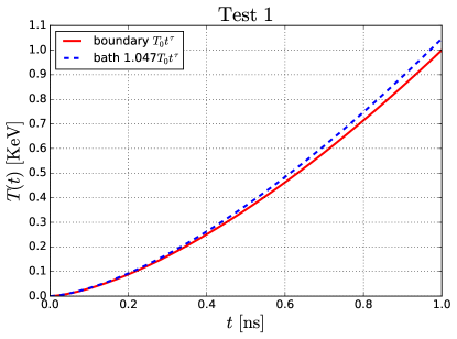
Figure 12: A comparison between the surface and bath drive temperatures for test 1.

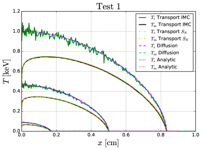
Figure 13: Radiation and material temperature profiles for Test 1. Results are shown at times $t=0.2,\ 0.6$ and 1ns, as obtained from the gray diffusion self-similar solution, a gray diffusion simulation and from Implicit-Monte-Carlo (IMC) and discrete ordinates ($S_{N}$) transport simulations.

We take $\alpha=\alpha^{\prime}=1.5$, $\lambda=\lambda^{\prime}=0.2$, $\mathcal{G}=0.025\frac{\text{cm}\left(\text{g}/\text{cm}^{3}\right)^{1.2}}{\text{keV}^{1.5}}$, $\mathcal{G}^{\prime}=10\frac{\text{cm$\left(\text{g}/\text{cm}^{3}\right)^{1.2}$}}{\text{keV}^{1.5}}$, so that the total and absorption opacities are:

$$k_{t}\left(T,\rho\right) =40\left(\frac{T}{\text{keV}}\right)^{-1.5}\left(\frac{\rho}{\text{g}/\text{cm}^{3}}\right)^{1.2}\ \text{cm}^{-1},$$

$$k_{a}\left(T,\rho\right) =0.1\left(\frac{T}{\text{keV}}\right)^{-1.5}\left(\frac{\rho}{\text{g}/\text{cm}^{3}}\right)^{1.2}\ \text{cm}^{-1}.$$

For transport simulations, the scattering opacity [Eq. (54)] is given by:

$$k_{s}\left(T,\rho\right) =39.9\left(\frac{T}{\text{keV}}\right)^{-1.5}\left(\frac{\rho}{\text{g}/\text{cm}^{3}}\right)^{1.2}\ \text{cm}^{-1},$$

which has the form of a power-law since the absorption and total opacities have the same temperature and density exponents. For the material energy density we take $\mu=0.14$, so that the critical exponent is $\beta_{c}=\beta_{c}^{\prime}=2.925$ [see Eqs. (34)-(35)]. We set $\beta=3.4$ and $\mathcal{F}=10^{14}\frac{\text{keV}^{-3.4}}{\left(\text{g}/\text{cm}^{3}\right)^{0.86}}\frac{\text{erg}}{\text{cm}^{3}}$, so that the material energy density is given by:

$$u\left(T,\rho\right)=10^{14}\left(\frac{T}{\text{keV}}\right)^{3.4}\left(\frac{\rho}{\text{g}/\text{cm}^{3}}\right)^{0.86}\ \text{{\hbox{\frac{\text{erg}}{\text{cm}^{3}}}}}.$$

For the exponents of this material model, using Eqs. (17)-(18), a self similar solution exists for a surface temperature temporal exponent $\tau=\frac{86}{57}\approx 1.50877$ and a spatial density exponent $\omega=-\frac{20}{19}\approx-1.05263$. Therefore, the surface temperature and the material density profile are:

$$T_{s}\left(t\right)=\left(\frac{t}{\text{ns}}\right)^{\frac{86}{57}}\ \text{keV},$$

$$\rho\left(x\right)=\left(\frac{x}{\text{cm}}\right)^{\frac{20}{19}}\ \text{g}/\text{cm}^{3}.$$

Using Eqs. (19)-(20), we find the dimensionless constants of the problem: $\mathcal{A}=1.75246$ and $\mathcal{B}=4.15619$. The similarity exponent is $\delta=1$, since the absorption and total opacities have the same exponents [see Eq. (24)] and the wave travels at constant speed. The numerical solution of the similarity equations (27)-(28) gives the heat front coordinate $\xi_{0}=1.2746051$, so that the heat front position, according to Eq. (30) is:

$$x_{F}\left(t\right)=0.8332614\left(\frac{t}{\text{ns}}\right)\ \text{cm}.$$

The resulting dimensionless flux at the origin is $\mathcal{S}\left(0\right)=4.62922$, so that the bath temperature is [Eq. (48)]:

$$T_{\text{bath}}\left(t\right)=1.0470478\left(\frac{t}{\text{ns}}\right)^{\frac{86}{57}}\ \text{keV},$$

which is used in transport simulations via the incoming bath radiation flux [Eq. (55)] or in diffusion simulations via the Marshak boundary condition [Eq. (44)]. We note that the bath temperature has a power law form since $\delta=1$. Diffusion simulations can be run, alternatively, using the surface temperature boundary condition [Eq. (7)]. A comparison of the surface and bath temperatures as a function of time is displayed in Fig. 12.

The radiation and material temperature profiles are given by the self-similar solution [Eqs. (25)-(26)]:

$$T_{r}\left(x,t\right)=\left(\frac{t}{\text{ns}}\right)^{\frac{86}{57}}f^{1/4}\left(\xi_{0}x/x_{F}\left(t\right)\right)\ \text{keV},$$

$$T\left(x,t\right)=\left(\frac{t}{\text{ns}}\right)^{\frac{86}{57}}g^{1/4}\left(\xi_{0}x/x_{F}\left(t\right)\right)\ \text{keV}.$$

As discussed in Sec. III, there is no analytical solution for the temperature profiles. The resulting numerical solution is tabulated in table 2. Simple closed form approximate expressions for the temperature profiles are given in table (3), with an accuracy which is better than $0.5$%. The profiles in tables 2 and 3 are given as functions of $\xi/\xi_{0}=x/x_{F}\left(t\right)$. As discussed in Sec. III.2, since we have $\beta<4$, the spatial density increases in space, and the material temperature is reduced to zero towards the origin.

Since $\mathcal{B}$ is not much larger than unity, we expect a significant deviation from equilibrium. This is seen in Fig. 13, where radiation and material temperature profiles of the self-similar gray diffusion solution are compared to the results of numerical gray diffusion and transport simulations.

TEST 2

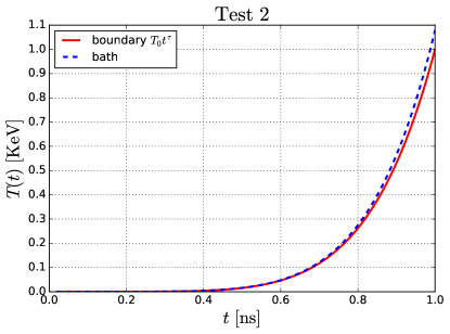
Figure 14: A comparison between the surface and bath drive temperatures for test 2.

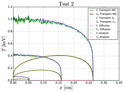
Figure 15: Radiation and material temperature profiles for Test 2. Results are shown at times $t=0.631385,\ 0.864201$ and 1ns, as obtained from a gray diffusion simulation and from Implicit-Monte-Carlo (IMC) and discrete ordinates ($S_{N}$) transport simulations.

We define, as in test 1, another case with $\omega<0$, but with a sharper heat front. We take $\alpha=3$, $\alpha^{\prime}=2$, $\lambda=0.2$, $\lambda^{\prime}=0.1$, $\mathcal{G}=10^{-3}\frac{\text{cm}\left(\text{g}/\text{cm}^{3}\right)^{1.2}}{\text{keV}^{3}}$, $\mathcal{G}^{\prime}=10\frac{\text{cm$\left(\text{g}/\text{cm}^{3}\right)^{1.1}$}}{\text{keV}^{2}}$, so that the total and absorption opacities are:

$$k_{t}\left(T,\rho\right) =10^{3}\left(\frac{T}{\text{keV}}\right)^{-3}\left(\frac{\rho}{\text{g}/\text{cm}^{3}}\right)^{1.2}\ \text{cm}^{-1},$$

$$k_{a}\left(T,\rho\right) =0.1\left(\frac{T}{\text{keV}}\right)^{-2}\left(\frac{\rho}{\text{g}/\text{cm}^{3}}\right)^{1.1}\ \text{cm}^{-1}.$$

For transport simulations, the scattering opacity [Eq. (54)] is given by:

$$k_{s}\left(T,\rho\right) =10^{3}\left(\frac{T}{\text{keV}}\right)^{-3}\left(\frac{\rho}{\text{g}/\text{cm}^{3}}\right)^{1.2}$$

$$-0.1\left(\frac{T}{\text{keV}}\right)^{-2}\left(\frac{\rho}{\text{g}/\text{cm}^{3}}\right)^{1.1}\ \text{cm}^{-1},$$

which is not a power-law form as in test 1, since the absorption and total opacities have different temperature and density exponents. We also take $\mu=0.4$, so that $\beta_{c}=2.909$ and $\beta_{c}^{\prime}=2.69565$. We set $\beta=3$ and $\mathcal{F}=10^{14}\frac{\text{keV}^{-3}}{\left(\text{g}/\text{cm}^{3}\right)^{0.6}}\frac{\text{erg}}{\text{cm}^{3}}$, so that the material energy density is given by:

$$u\left(T,\rho\right)=10^{14}\left(\frac{T}{\text{keV}}\right)^{3}\left(\frac{\rho}{\text{g}/\text{cm}^{3}}\right)^{0.6}\ \text{{\hbox{\frac{\text{erg}}{\text{cm}^{3}}}}}.$$

For the exponents of this material model we get $\tau=6$ and $\omega=-\frac{20}{7}\approx-2.8571$, so that the surface temperature and density profile are:

$$T_{s}\left(t\right)=\left(\frac{t}{\text{ns}}\right)^{6}\ \text{keV},$$

$$\rho\left(x\right)=\left(\frac{x}{\text{cm}}\right)^{\frac{20}{7}}\ \text{g}/\text{cm}^{3}.$$

The dimensionless constants of the problem are $\mathcal{A}=0.20833$ and $\mathcal{B}=1.63201$. As in the previous case, $\mathcal{B}$ is not large and we expect a significant deviation from equilibrium. From Eq. (24) we find the similarity exponent $\delta=\frac{7}{2}$, so that the the wave front accelerates over time. The resulting numerical heat front similarity coordinate is $\xi_{0}=0.615503394$, so that the heat front position is:

$$x_{F}\left(t\right)=0.26348387\left(\frac{t}{\text{ns}}\right)^{\frac{7}{2}}\ \text{cm}.$$

The resulting numerical dimensionless flux at the origin is $\mathcal{S}\left(0\right)=12.5696$, so that the bath temperature is [Eq. (48)]:

$$T_{\text{bath}}\left(t\right)=\left(1+0.358968\left(\frac{t}{\text{ns}}\right)^{\frac{5}{2}}\right)^{\frac{1}{4}}\left(\frac{t}{\text{ns}}\right)^{6}\ \text{keV},$$

which is not in a power law form, since $\delta\neq 1$. A comparison of the surface and bath temperatures as a function of time is displayed in Fig. 14.

The radiation and material temperature profiles are given by the self-similar solution [Eqs. (25)-(26)]:

$$T_{r}\left(x,t\right)=\left(\frac{t}{\text{ns}}\right)^{6}f^{1/4}\left(\xi_{0}x/x_{F}\left(t\right)\right)\ \text{keV},$$

$$T\left(x,t\right)=\left(\frac{t}{\text{ns}}\right)^{6}g^{1/4}\left(\xi_{0}x/x_{F}\left(t\right)\right)\ \text{keV}.$$

The resulting numerical profiles are tabulated in table 2 and approximate closed form expressions are given in table (3) as a function of $\xi/\xi_{0}=x/x_{F}\left(t\right)$. As in the previous case, since we have $\beta<4$, the material temperature is decreased to zero towards the origin.

The temperature profiles are displayed in Fig. 15, showing again a great agreement between the various simulations and analytic gray diffusion solution.

TEST 3

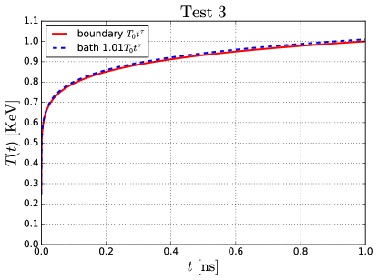
Figure 16: A comparison between the surface and bath drive temperatures for test 3.

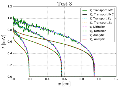
Figure 17: Radiation and material temperature profiles for Test 3. Results are shown at times $t=0.2,\ 0.6$ and 1ns, as obtained from the gray diffusion self-similar solution, a gray diffusion simulation and from Implicit-Monte-Carlo (IMC) and discrete ordinates ($S_{N}$) transport simulations.

We now define a case with $\omega>0$. We take $\alpha=\alpha^{\prime}=4.5$, $\lambda=\lambda^{\prime}=0.9$, $\mathcal{G}=0.5\frac{\text{cm}\left(\text{g}/\text{cm}^{3}\right)^{1.9}}{\text{keV}^{4.5}}$, $\mathcal{G}^{\prime}=10^{3}\frac{\text{cm$\left(\text{g}/\text{cm}^{3}\right)^{1.9}$}}{\text{keV}^{4.5}}$, so that the total and absorption opacities are:

$$k_{t}\left(T,\rho\right) =2\left(\frac{T}{\text{keV}}\right)^{-4.5}\left(\frac{\rho}{\text{g}/\text{cm}^{3}}\right)^{1.9}\ \text{cm}^{-1},$$

$$k_{a}\left(T,\rho\right) =10^{-3}\left(\frac{T}{\text{keV}}\right)^{-4.5}\left(\frac{\rho}{\text{g}/\text{cm}^{3}}\right)^{1.9}\ \text{cm}^{-1}.$$

For transport simulations, the scattering opacity is given by a power law form as well:

$$k_{s}\left(T,\rho\right) =1.999\left(\frac{T}{\text{keV}}\right)^{-4.5}\left(\frac{\rho}{\text{g}/\text{cm}^{3}}\right)^{1.9}\ \text{cm}^{-1}.$$

We also take $\mu=0.3$, so that $\beta_{c}=\beta_{c}^{\prime}=2.3421$. We set $\beta=6$ and $\mathcal{F}=10^{14}\frac{\text{keV}^{-6}}{\left(\text{g}/\text{cm}^{3}\right)^{0.7}}\frac{\text{erg}}{\text{cm}^{3}}$, so that the material energy density is given by:

$$u\left(T,\rho\right)=10^{14}\left(\frac{T}{\text{keV}}\right)^{6}\left(\frac{\rho}{\text{g}/\text{cm}^{3}}\right)^{0.7}\ \text{{\hbox{\frac{\text{erg}}{\text{cm}^{3}}}}}.$$

For the exponents of this material model, we find $\tau=\frac{14}{139}\approx 0.10072$ and $\omega=\frac{40}{139}\approx 0.28777$, so that the surface temperature and density profile are:

$$T_{s}\left(t\right)=\left(\frac{t}{\text{ns}}\right)^{\frac{14}{139}}\ \text{keV},$$

$$\rho\left(x\right)=\left(\frac{x}{\text{cm}}\right)^{-\frac{40}{139}}\ \text{g}/\text{cm}^{3}.$$

The dimensionless constants of the problem are $\mathcal{A}=0.0163665$ and $\mathcal{B}=0.0187098$, so we expect a significant deviation from equilibrium. As in test 1, the similarity exponent is $\delta=1$, since the absorption and total opacities have the same exponents. The resulting numerical heat front similarity coordinate is $\xi_{0}=0.31411518$, so that the heat front position is

$$x_{F}\left(t\right)=0.95029077\left(\frac{t}{\text{ns}}\right)\ \text{cm}.$$

The resulting numerical dimensionless flux at the origin is $\mathcal{S}\left(0\right)=0.20284$, so that the bath temperature is [Eq. (48)]:

$$T_{\text{bath}}\left(t\right)=1.01008116\left(\frac{t}{\text{ns}}\right)^{\frac{14}{139}}\ \text{keV}.$$

A comparison of the surface and bath temperatures as a function of time is displayed in Fig. 16.

The radiation and material temperature profiles are given by the self-similar solution [Eqs. (25)-(26)]:

$$T_{r}\left(x,t\right)=\left(\frac{t}{\text{ns}}\right)^{\frac{14}{139}}f^{1/4}\left(\xi_{0}x/x_{F}\left(t\right)\right)\ \text{keV},$$

$$T\left(x,t\right)=\left(\frac{t}{\text{ns}}\right)^{\frac{14}{139}}g^{1/4}\left(\xi_{0}x/x_{F}\left(t\right)\right)\ \text{keV}.$$

The resulting numerical profiles are tabulated in table 2 and approximate closed form expressions are given in table (3) as a function of $\xi/\xi_{0}=x/x_{F}\left(t\right)$. In this case, since we have $\beta>4$, the material temperature is equal to the radiation temperature at the origin.

The temperature profiles are displayed in Fig. 17, showing again a great agreement between the various simulations and analytic gray diffusion solution.

TEST 4

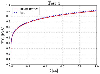
Figure 18: A comparison between the surface and bath drive temperatures for test 4.

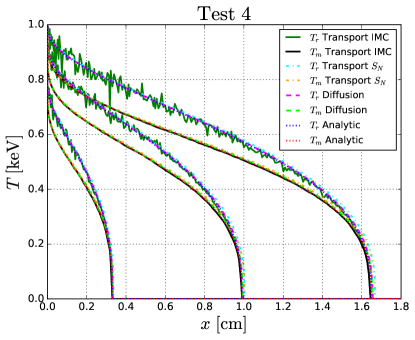
Figure 19: Radiation and material temperature profiles for Test 4. Results are shown at times $t=0.233846,\ 0.630525$ and 1ns, as obtained from the gray diffusion self-similar solution, a gray diffusion simulation and from Implicit-Monte-Carlo (IMC) and discrete ordinates ($S_{N}$) transport simulations.

We define, as in test 3, a test with $\omega>0$ but with a less steep heat front. We take, as in test 2 the exponents $\alpha=3$, $\alpha^{\prime}=2$, $\lambda=0.2$, $\lambda^{\prime}=0.1$ and $\mathcal{G}=0.5\frac{\text{cm}\left(\text{g}/\text{cm}^{3}\right)^{1.2}}{\text{keV}^{3}}$, $\mathcal{G}^{\prime}=10^{2}\frac{\text{cm$\left(\text{g}/\text{cm}^{3}\right)^{1.1}$}}{\text{keV}^{2}}$, so that the total and absorption opacities are:

$$k_{t}\left(T,\rho\right) =2\left(\frac{T}{\text{keV}}\right)^{-3}\left(\frac{\rho}{\text{g}/\text{cm}^{3}}\right)^{1.2}\ \text{cm}^{-1},$$

$$k_{a}\left(T,\rho\right) =10^{-2}\left(\frac{T}{\text{keV}}\right)^{-2}\left(\frac{\rho}{\text{g}/\text{cm}^{3}}\right)^{1.1}\ \text{cm}^{-1}.$$

For transport simulations, the scattering opacity [Eq. (54)] is given by:

$$k_{s}\left(T,\rho\right) =2\left(\frac{T}{\text{keV}}\right)^{-3}\left(\frac{\rho}{\text{g}/\text{cm}^{3}}\right)^{1.2}$$

$$-10^{-2}\left(\frac{T}{\text{keV}}\right)^{-2}\left(\frac{\rho}{\text{g}/\text{cm}^{3}}\right)^{1.1}\ \text{cm}^{-1}.$$

We also take $\mu=0.4$, so that $\beta_{c}=2.909$ and $\beta_{c}^{\prime}=2.69565$. We set $\beta=6.5$ and $\mathcal{F}=10^{14}\frac{\text{keV}^{-6.5}}{\left(\text{g}/\text{cm}^{3}\right)^{0.6}}\frac{\text{erg}}{\text{cm}^{3}}$, so that the material energy density is given by:

$$u\left(T,\rho\right)=10^{14}\left(\frac{T}{\text{keV}}\right)^{6.5}\left(\frac{\rho}{\text{g}/\text{cm}^{3}}\right)^{0.6}\ \text{{\hbox{\frac{\text{erg}}{\text{cm}^{3}}}}}.$$

For the exponents of this material model we get $\tau=\frac{12}{79}\approx 0.151899$ and $\omega=\frac{4}{7}\approx 0.571429$, so that the surface temperature and density profile are:

$$T_{s}\left(t\right)=\left(\frac{t}{\text{ns}}\right)^{\frac{12}{79}}\ \text{keV},$$

$$\rho\left(x\right)=\left(\frac{x}{\text{cm}}\right)^{-\frac{4}{7}}\ \text{g}/\text{cm}^{3}.$$

The dimensionless constants of the problem are $\mathcal{A}=0.138891$ and $\mathcal{B}=0.178419$. As in the previous case, $\mathcal{B}$ is not large and we expect a significant deviation from equilibrium. From Eq. (24) we find the similarity exponent $\delta=\frac{175}{158}\approx 1.10759$, so that the the wave front accelerates over time. The resulting numerical heat front similarity coordinate is $\xi_{0}=0.48463864$ and the heat front position is:

$$x_{F}\left(t\right)=1.648216882\left(\frac{t}{\text{ns}}\right)^{\frac{175}{158}}\ \text{cm}.$$

The resulting numerical dimensionless flux at the origin is $\mathcal{S}\left(0\right)=0.260125$, so that the bath temperature is [Eq. (48)]:

$$T_{\text{bath}}\left(t\right)=\left(1+0.0590184\left(\frac{t}{\text{ns}}\right)^{\frac{17}{158}}\right)^{\frac{1}{4}}\left(\frac{t}{\text{ns}}\right)^{\frac{12}{79}}\ \text{keV}.$$

A comparison of the surface and bath temperatures as a function of time is displayed in Fig. 18.

The radiation and material temperature profiles are given by the self-similar solution [Eqs. (25)-(26)]:

$$T_{r}\left(x,t\right)=\left(\frac{t}{\text{ns}}\right)^{\frac{12}{79}}f^{1/4}\left(\xi_{0}x/x_{F}\left(t\right)\right)\ \text{keV},$$

$$T\left(x,t\right)=\left(\frac{t}{\text{ns}}\right)^{\frac{12}{79}}g^{1/4}\left(\xi_{0}x/x_{F}\left(t\right)\right)\ \text{keV}.$$

The resulting numerical profiles are tabulated in table 2 and approximate closed form expressions are given in table (3) as a function of $\xi/\xi_{0}=x/x_{F}\left(t\right)$. As in the previous case, since we have $\beta>4$, the material temperature is equal to the radiation temperature at the origin.

The temperature profiles are displayed in Fig. 19, showing again a great agreement between the various simulations and analytic gray diffusion solution.

TEST 5

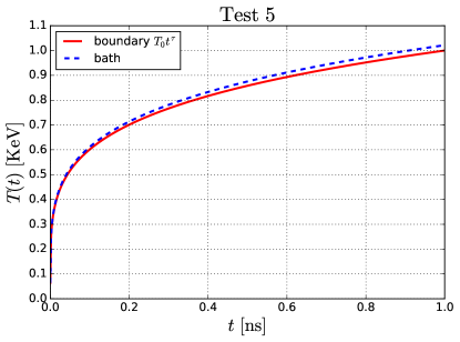
Figure 20: A comparison between the surface and bath drive temperatures for test 5.

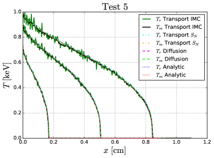
Figure 21: Radiation and material temperature profiles for Test 5. Results are shown at times $t=0.2346891,\ 0.63124555$ and 1ns, as obtained from the gray diffusion self-similar solution, a gray diffusion simulation and from Implicit-Monte-Carlo (IMC) and discrete ordinates ($S_{N}$) transport simulations.

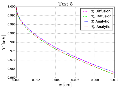
Figure 22: A close view near the origin of the temperature profiles at time $t=1\text{ns}$ (from the gray diffusion simulation and analytic solution), for Test 5 (see Fig. 21).

We define another case with $\omega>0$, and such that $\mathcal{B}\gg 1$, so that the thermodynamic equilibrium limit is reached, unlike the previous cases which were significantly out of equilibrium. We take $\alpha=3$, $\alpha^{\prime}=2$, $\lambda=\lambda^{\prime}=0.35$, $\mathcal{G}=0.2\frac{\text{cm}\left(\text{g}/\text{cm}^{3}\right)^{1.35}}{\text{keV}^{3}}$, $\mathcal{G}^{\prime}=0.2\frac{\text{cm$\left(\text{g}/\text{cm}^{3}\right)^{1.35}$}}{\text{keV}^{2}}$, so that the total and absorption opacities are:

$$k_{t}\left(T,\rho\right) =5\left(\frac{T}{\text{keV}}\right)^{-3}\left(\frac{\rho}{\text{g}/\text{cm}^{3}}\right)^{1.35}\ \text{cm}^{-1},$$

$$k_{a}\left(T,\rho\right) =5\left(\frac{T}{\text{keV}}\right)^{-2}\left(\frac{\rho}{\text{g}/\text{cm}^{3}}\right)^{1.35}\ \text{cm}^{-1}.$$

For transport simulations, the scattering opacity [Eq. (54)] is given by:

$$k_{s}\left(T,\rho\right) =5\left(\frac{\rho}{\text{g}/\text{cm}^{3}}\right)^{1.35}\left[\left(\frac{T}{\text{keV}}\right)^{-3}-\left(\frac{T}{\text{keV}}\right)^{-2}\right]\ \text{cm}^{-1}.$$

We also take $\mu=0.2$, so that $\beta_{c}=2.8148$ and $\beta_{c}^{\prime}=2.5185$. We set $\beta=5.5$ and $\mathcal{F}=2\times 10^{14}\frac{\text{keV}^{-5.5}}{\left(\text{g}/\text{cm}^{3}\right)^{0.8}}\frac{\text{erg}}{\text{cm}^{3}}$, so that the material energy density is given by:

$$u\left(T,\rho\right)=2\times 10^{14}\left(\frac{T}{\text{keV}}\right)^{5.5}\left(\frac{\rho}{\text{g}/\text{cm}^{3}}\right)^{0.8}\ \text{{\hbox{\frac{\text{erg}}{\text{cm}^{3}}}}}.$$

For the exponents of this material model we get $\tau=\frac{32}{145}\approx 0.22069$ and $\omega=\frac{60}{161}\approx 0.372671$, so that the surface temperature and density profile are:LTE

$$T_{s}\left(t\right)=\left(\frac{t}{\text{ns}}\right)^{\frac{32}{145}}\ \text{keV},$$

$$\rho\left(x\right)=\left(\frac{x}{\text{cm}}\right)^{-\frac{60}{161}}\ \text{g}/\text{cm}^{3}.$$

The dimensionless constants of the problem are $\mathcal{A}=118.772$ and $\mathcal{B}=68.0203$. Since $\mathcal{B}$ significantly larger than unity, we expect the material and radiation temperatures to be very close (and, as in tests 3-4, equal at the origin, since $\omega>0$). From Eq. (24) we find the similarity exponent $\delta=\frac{161}{145}\approx 1.11034$, so that the the wave front accelerates over time. The resulting numerical heat front similarity coordinate is $\xi_{0}=0.53073002$ and the heat front position is:

$$x_{F}\left(t\right)=0.8428997\left(\frac{t}{\text{ns}}\right)^{\frac{161}{145}}\ \text{cm}.$$

The resulting numerical dimensionless flux at the origin is $\mathcal{S}\left(0\right)=0.840029$, so that the bath temperature is [Eq. (48)]:

$$T_{\text{bath}}\left(t\right)=\left(1+0.0890032\left(\frac{t}{\text{ns}}\right)^{\frac{16}{145}}\right)^{\frac{1}{4}}\left(\frac{t}{\text{ns}}\right)^{\frac{32}{145}}\ \text{keV}.$$

A comparison of the surface and bath temperatures as a function of time is displayed in Fig. 20.

The radiation and material temperature profiles are given by the self-similar solution [Eqs. (25)-(26)]:

$$T_{r}\left(x,t\right)=\left(\frac{t}{\text{ns}}\right)^{\frac{32}{145}}f^{1/4}\left(\xi_{0}x/x_{F}\left(t\right)\right)\ \text{keV},$$

$$T\left(x,t\right)=\left(\frac{t}{\text{ns}}\right)^{\frac{32}{145}}g^{1/4}\left(\xi_{0}x/x_{F}\left(t\right)\right)\ \text{keV}.$$

The resulting numerical profiles are tabulated in table 2 and approximate closed form expressions are given in table (3) as a function of $\xi/\xi_{0}=x/x_{F}\left(t\right)$.

The temperature profiles are displayed in Fig. 21, showing again a great agreement between the various simulations and analytic gray diffusion solution. It is evident that resulting temperature profiles are very close to a state of equilibrium, as the radiation and material temperatures differ by about $0.1\%$. This difference, is evident in Fig. 22, where we show a close up view near the origin. It is interesting to see the great agreement of the gray diffusion simulations with the analytic solution even on that scale.

TEST 6

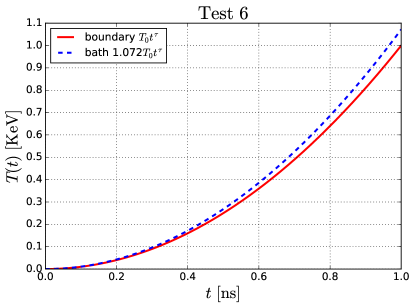
Figure 23: A comparison between the surface and bath drive temperatures for test 6.

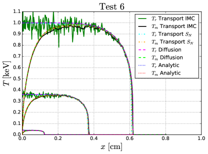
Figure 24: Radiation and material temperature profiles for Test 6. Results are shown at times $t=0.2,\ 0.6$ and 1ns, as obtained from the gray diffusion self-similar solution, a gray diffusion simulation and from Implicit-Monte-Carlo (IMC) and discrete ordinates ($S_{N}$) transport simulations.

We define the last case to have $\omega=-3$, and $\mathcal{B}\gg 1$, so that the thermodynamic equilibrium limit should be reached. We set a material with free-free like absorption, which depends on $\rho^{2}$. Since $\rho\left(x\right)\propto x^{3}$, the density, and as a result, the coupling between the material and radiation, is expected to be very low in a wide region near the origin. This results in a significant state of non-equilibrium ranging from the origin and halfway towards the front (where the coupling is large due to the lower material temperature). We take $\alpha=\alpha^{\prime}=3.5$, $\lambda=\lambda^{\prime}=1$, $\mathcal{G}=0.0005\frac{\text{cm}\left(\text{g}/\text{cm}^{3}\right)^{2}}{\text{keV}^{3.5}}$, $\mathcal{G}^{\prime}=0.01\frac{\text{cm$\left(\text{g}/\text{cm}^{3}\right)^{2}$}}{\text{keV}^{3.5}}$, so that the total and absorption opacities are:

$$k_{t}\left(T,\rho\right) =2000\left(\frac{T}{\text{keV}}\right)^{-3.5}\left(\frac{\rho}{\text{g}/\text{cm}^{3}}\right)^{2}\ \text{cm}^{-1},$$

$$k_{a}\left(T,\rho\right) =100\left(\frac{T}{\text{keV}}\right)^{-3.5}\left(\frac{\rho}{\text{g}/\text{cm}^{3}}\right)^{2}\ \text{cm}^{-1}.$$

For transport simulations, the scattering opacity [Eq. (54)] is given by:

$$k_{s}\left(T,\rho\right) =1900\left(\frac{T}{\text{keV}}\right)^{-3.5}\left(\frac{\rho}{\text{g}/\text{cm}^{3}}\right)^{2}\ \text{cm}^{-1}.$$

We take and ideal like energy density, $\mu=0$, so that $\beta_{c}=\beta_{c}^{\prime}=2.25$. We set $\beta=2.5$ and $\mathcal{F}=10^{14}\frac{\text{keV}^{-2.5}}{\text{g}/\text{cm}^{3}}\frac{\text{erg}}{\text{cm}^{3}}$, so that the material energy density is given by:

$$u\left(T,\rho\right)=10^{14}\left(\frac{T}{\text{keV}}\right)^{2.5}\left(\frac{\rho}{\text{g}/\text{cm}^{3}}\right)\ \text{{\hbox{\frac{\text{erg}}{\text{cm}^{3}}}}}.$$

For the exponents of this material model we get $\tau=2$ and a $\omega=-3$, so that the surface temperature and density profile are:

$$T_{s}\left(t\right)=\left(\frac{t}{\text{ns}}\right)^{2}\ \text{keV},$$

$$\rho\left(x\right)=\left(\frac{x}{\text{cm}}\right)^{3}\ \text{g}/\text{cm}^{3}.$$

The dimensionless constants of the problem are $\mathcal{A}=56.3408$ and $\mathcal{B}=902.197$. The resulting similarity exponent is $\delta=1$, and the numerical heat front coordinate is $\xi_{0}=1.19867771$, so that the heat front position is:

$$x_{F}\left(t\right)=0.61806779\left(\frac{t}{\text{ns}}\right)\ \text{cm}.$$

The resulting numerical dimensionless flux at the origin is $\mathcal{S}\left(0\right)=9.31253$, so that the bath temperature is [Eq. (48)]:

$$T_{\text{bath}}\left(t\right)=1.0719423\left(\frac{t}{\text{ns}}\right)^{2}\ \text{keV}.$$

A comparison of the surface and bath temperatures as a function of time is displayed in Fig. 23.

The radiation and material temperature profiles are given by the self-similar solution [Eqs. (25)-(26)]:

$$T_{r}\left(x,t\right)=\left(\frac{t}{\text{ns}}\right)^{2}f^{1/4}\left(\xi_{0}x/x_{F}\left(t\right)\right)\ \text{keV},$$

$$T\left(x,t\right)=\left(\frac{t}{\text{ns}}\right)^{2}g^{1/4}\left(\xi_{0}x/x_{F}\left(t\right)\right)\ \text{keV}.$$

The resulting numerical profiles are tabulated in table 2 and approximate closed form expressions are given in table (3) as a function of $\xi/\xi_{0}=x/x_{F}\left(t\right)$. The temperature profiles are displayed in Fig. 24, showing again a great agreement between the various simulations and analytic gray diffusion solution. We note the significant lack of equilibrium in a wide range near the origin.

V Conclusion

In this work we have developed new self-similar solutions to a nonlinear non-equilibrium supersonic Marshak wave problem in non-homogeneous media in the diffusion limit of radiative transfer. The solutions exist under the assumptions of a temporal power-law surface radiation temperature drive of the form $T_{s}\left(t\right)=T_{0}t^{\tau}$, a spatial power law density profile $\rho\left(x\right)=\rho_{0}x^{-\omega}$, and material model with power law temperature and density dependent total and absorption opacities $k_{t}\left(T,\rho\right)=\frac{1}{g}T^{-\alpha}\rho^{\lambda+1}$ and $k_{a}\left(T,\rho\right)=\frac{1}{g^{\prime}}T^{-\alpha^{\prime}}\rho^{\lambda^{\prime}+1}$, and a material energy density $u\left(T,\rho\right)=\mathcal{F}T^{\beta}\rho^{1-\mu}$. The solutions are a generalization of the recent work [27], were such non-linear non-equilibrium solutions were developed for a homogeneous media ($\omega=0$), which required a material energy density that is proportional to the radiation energy density ($\beta=4$). It is shown that the generalized solutions exist for specific values of the temporal drive exponent $\tau$ and the spatial density exponent $\omega$, which are functions of the temperature and density material model exponents $\alpha,\lambda,\alpha^{\prime},\lambda^{\prime},\beta,\mu$ (given by Eqs. (17)-(18)). The properties of the solutions were analyzed in detail, including the range of validity and the thermodynamic equilibrium limit for which the radiation and material temperature become very close. The behavior of the solutions near the origin was analyzed, and it was shown that the material temperature at the origin is always zero for $\omega<0$; can have any value between 0 and the radiation temperature for $\omega=0$; and is always equal to the radiation temperature when $\omega>0$.

We constructed a set of non-equilibrium and non-homogeneous Marshak wave benchmarks for supersonic radiative heat transfer. The numerical solutions of the similarity profiles for these benchmarks were tabulated, and approximate closed form analytic functions were also given for convenience. The benchmarks were run using implicit Monte-Carlo and discrete-ordinate radiation transport simulations as well gray diffusion simulations. All benchmarks, which were defined to be optically thick, resulted in a very good agreement with the similarity solutions of the gray diffusion equation. We conclude that the solutions developed in this work can be used as non-trivial but easy to implement code verification test problems for non-equilibrium radiation heat transfer computer simulations.

Availability of data

The data that support the findings of this study are available from the corresponding author upon reasonable request.

Appendix A Dimensional analysis

$E$	$U$	$E_{0}$	$K$	$M$	$P$	$x$	$t$
$\left[E\right]$	$\left[E\right]$	$\frac{\left[E\right]}{\left[\text{time}\right]^{4\tau}}$	$\frac{\left[\text{length}\right]^{2-\omega\left(1+\lambda\right)}}{\left[E\right]^{\frac{\alpha}{4}}\left[\text{time}\right]}$	$\frac{\left[E\right]{}^{\frac{\alpha^{\prime}}{4}}\left[\text{length}\right]^{\omega\left(1+\lambda^{\prime}\right)}}{\left[\text{time}\right]}$	$\frac{\left[E\right]^{\frac{\alpha^{\prime}+\beta}{4}-1}\left[\text{length}\right]^{\omega\left(\lambda^{\prime}+\mu\right)}}{\left[\text{time}\right]}$	$\left[\text{length}\right]$	$\left[\text{time}\right]$

Table 4: The dimensional quantities in the problem (upper line) and their dimensions (lower line). $\left[E\right]$ denotes the dimensions of energy per unit volume.

In this appendix, we use the method of dimensional analysis to construct a self-similar solution of the problem defined by the nonlinear gray diffusion model in Eqs. (12)-(13), with the initial and boundary conditions (5)-(8). As detailed in table 4, the problem is formulated in terms $8$ dimensional quantities, which are composed of $3$ different units - time, length and energy density. According the the Pi (Buckingham) theorem of dimensional analysis [71, 32, 72], the problem can be expressed in terms of $8-3=5$ dimensionless variables $\Pi_{1},\Pi_{2},\Pi_{3},\Pi_{4},\Pi_{5}$ which are defined as products of power laws in terms of the dimensional quantities. In order to express the solution with a single similarity independent variable $\Pi_{1}=\xi$ and two self-similar dependent variables for the radiation $\Pi_{2}=f\left(\xi\right)\propto E$ and matter $\Pi_{3}=g\left(\xi\right)\propto U$, we require that the remaining dimensionless quantities, which we denote as $\mathcal{A}=\Pi_{4}$, $\mathcal{B}=\Pi_{5}$, would not depend on $E,U,x,t$, that is, they should be dimensionless quantities that depend on the dimensional constants characterizing the problem, which we write as:

$$\Pi_{4} =\mathcal{A}=E_{0}^{n}K^{k}M^{m},$$ (58)

$$\Pi_{5} =\mathcal{B}=E_{0}^{n^{\prime}}K^{k^{\prime}}P^{p}.$$ (59)

The requirement that $\mathcal{A}$ is dimensionless results in the following homogeneous system of linear equations:

$$n-\frac{\alpha}{4}k+\frac{\alpha^{\prime}}{4}m=0,$$

$$k\left(2-\omega\left(1+\lambda\right)\right)+m\omega\left(1+\lambda^{\prime}\right)=0,$$

$$4\tau n+k+m=0,$$

which has the solution:

$$k\left(2-\omega\left(1+\lambda\right)-\omega\frac{1+\alpha\tau}{1-\alpha^{\prime}\tau}\left(1+\lambda^{\prime}\right)\right)=0,$$

$$n=-\frac{1}{4\tau}\left(k+m\right),$$

$$m=-\frac{1+\alpha\tau}{1-\alpha^{\prime}\tau}k.$$

A set of infinite non-trivial solutions exists only if:

$$\frac{\omega\left(1+\lambda^{\prime}\right)}{2-\omega\left(1+\lambda\right)}=\frac{1-\alpha^{\prime}\tau}{1+\alpha\tau}.$$ (60)

By setting (without loss of generality) $m=1$, we have $n=-\frac{1}{1+\alpha\tau}\frac{\alpha+\alpha^{\prime}}{4},\,k=-\frac{1-\alpha^{\prime}\tau}{1+\alpha\tau}$ so that:

$$\mathcal{A}=E_{0}^{-\frac{\alpha+\alpha^{\prime}}{4\left(\alpha\tau+1\right)}}K^{\frac{\alpha^{\prime}\tau-1}{\alpha\tau+1}}M.$$ (61)

Similarly, by the requirement that $\mathcal{B}$ is dimensionless, we get the linear homogeneous system:

$$n^{\prime}-\frac{\alpha}{4}k^{\prime}+\left(\frac{\alpha^{\prime}+\beta}{4}-1\right)p=0,$$

$$k^{\prime}\left(2-\omega\left(1+\lambda\right)\right)+\omega p\left(\lambda^{\prime}+\mu\right)=0,$$

$$4\tau n^{\prime}+k^{\prime}+p=0,$$

which has the solution:

$$\left[\left(2-\omega\left(1+\lambda\right)\right)-\frac{1+\alpha\tau}{1-\left(\alpha^{\prime}+\beta-4\right)\tau}\omega\left(\lambda^{\prime}+\mu\right)\right]k^{\prime}=0,$$

$$p=-\frac{1+\alpha\tau}{1-\left(\alpha^{\prime}+\beta-4\right)\tau}k^{\prime},$$

$$n^{\prime}=-\frac{1}{4\tau}\left(k^{\prime}+p\right).$$

As before, an infinite set of nontrivial solutions exists only if:

$$\left(1-\left(\alpha^{\prime}+\beta-4\right)\tau\right)\left(2-\omega\left(1+\lambda\right)\right)$$

$$-\omega\left(1+\alpha\tau\right)\left(\lambda^{\prime}+\mu\right) =0$$ (62)

By solving Eqs. (60), (62) for $\tau$ and $\omega$, we obtain Eqs. (17)-(18). Therefore, given a material model which is defined by the exponents $\alpha,$$\lambda,$$\alpha^{\prime},$$\lambda^{\prime},$$\beta,$$\mu$, a self-similar solution exists only for a temporal exponent $\tau$ and spatial exponent $\omega$ which obey the relations Eqs. (17)-(18), respectively. By setting (without loss of generality) $p=1$, we get:

$$\mathcal{B}=E_{0}^{\frac{4-\beta-\alpha-\alpha^{\prime}}{4\left(\alpha\tau+1\right)}}K^{\frac{\left(\alpha^{\prime}+\beta-4\right)\tau-1}{\alpha\tau+1}}P.$$ (63)

We now write the dimensionless independent similarity coordinate as:

$$\Pi_{1}=\xi=xt^{-\delta}E_{0}^{n}K^{k}.$$ (64)

The requirement that $\xi$ is dimensionless results in the following (non-homogeneous) system of linear equations:

$$k\left(2-\omega\left(1+\lambda\right)\right)=-1,$$

$$n-\frac{\alpha}{4}k=0,$$

$$4\tau n+k+\delta=0.$$

which has the solution:

$$\delta=\frac{1+\alpha\tau}{2-\omega\left(1+\lambda\right)},$$

$$n=-\frac{\alpha}{4\left(2-\omega\left(1+\lambda\right)\right)},$$

$$k=-\frac{1}{2-\omega\left(1+\lambda\right)},$$

which proves Eq. (23). Finally, we can write the dimensionless similarity profiles directly, since the radiation energy density at the system boundary, $E_{0}t^{4\tau}$, has units of energy density:

$$\Pi_{2}=\frac{E}{E_{0}t^{4\tau}}=f\left(\xi\right),$$ (65)

$$\Pi_{3}=\frac{U}{E_{0}t^{4\tau}}=g\left(\xi\right).$$ (66)

We will now show explicitly, that by substituting the self-similar ansatz Eqs. (64),(65)-(66) in the gray diffusion equations (12)-(13), under the constrains Eqs. (17)-(18), results in a dimensionless ODE system for the similarity profiles $f,g$. By using the relation $\frac{\partial}{\partial x}=\frac{\xi}{x}\frac{\partial}{\partial\xi}$, the flux term in Eq. (12) reads:

$$\frac{\partial}{\partial x}\left(x^{\omega\left(1+\lambda\right)}U^{\frac{\alpha}{4}}\frac{\partial}{\partial x}E\right) =x^{\omega\left(1+\lambda\right)-2}\xi t^{\left(\alpha+4\right)\tau}E_{0}^{\frac{\alpha}{4}+1}\times$$

$$\Bigg{(}\omega\left(1+\lambda\right)g^{\frac{\alpha}{4}}f^{\prime}+\xi g^{\frac{\alpha}{4}-1}\left[\frac{\alpha}{4}f^{\prime}g^{\prime}+gf^{\prime\prime}\right]\Bigg{)}.$$ (67)

Similarly, by using the relation $\frac{\partial}{\partial t}=-\delta\frac{\xi}{t}\frac{\partial}{\partial\xi}$ the left hand side of Eq. (12) reads:

$$\frac{\partial E}{\partial t} =E_{0}t^{4\tau-1}\left(4\tau f-\delta\xi f^{\prime}\right).$$ (68)

By substituting Eqs. (67)-(68) in Eq. (12), we find:

$$E_{0}t^{4\tau-1}\left(4\tau f-\delta\xi f^{\prime}\right)=E_{0}t^{4\tau-1}\xi^{\omega\left(1+\lambda\right)}\times$$

$$\left(\frac{1}{\xi}\omega\left(1+\lambda\right)g^{\frac{\alpha}{4}}f^{\prime}+g^{\frac{\alpha}{4}-1}\left[\frac{\alpha}{4}f^{\prime}g^{\prime}+gf^{\prime\prime}\right]\right)$$

$$+ME_{0}^{-\frac{\alpha^{\prime}}{4}}\xi^{-\omega\left(1+\lambda^{\prime}\right)}\left(\frac{1}{t^{1+\alpha\tau}E_{0}^{\frac{\alpha}{4}}K}\right)^{\frac{\omega\left(1+\lambda^{\prime}\right)}{2-\omega\left(1+\lambda\right)}}\times$$

$$E_{0}g^{-\frac{\alpha^{\prime}}{4}}t^{\left(4-\alpha^{\prime}\right)\tau}\left(g-f\right).$$

By using Eq. (61), the dimensional quantity $M$ can be written in terms of the dimensionless $\mathcal{A}$, and by using Eq. (60), we find:

$$E_{0}t^{4\tau-1}\left(4\tau f-\delta\xi f^{\prime}\right) =E_{0}t^{4\tau-1}\xi^{\omega\left(1+\lambda\right)}\times$$

$$\Bigg{(}\frac{1}{\xi}\omega\left(1+\lambda\right)g^{\frac{\alpha}{4}}f^{\prime} +g^{\frac{\alpha}{4}-1}\left[\frac{\alpha}{4}f^{\prime}g^{\prime}+gf^{\prime\prime}\right]\Bigg{)}$$

$$+E_{0}t^{4\tau-1}\mathcal{A} \xi^{-\omega\left(1+\lambda^{\prime}\right)}g^{-\frac{\alpha^{\prime}}{4}}\left(g-f\right),$$

which upon factoring out the common dimensional $E_{0}t^{4\tau-1}$ term, results in the dimensionless similarity ODE (27). Similarly, the material equation (13) can be written as:

$$E_{0}t^{4\tau-1}\left(4\tau f-\delta\xi f^{\prime}\right) =P\xi^{-\omega\left(\mu+\lambda^{\prime}\right)}\left(\frac{1}{t^{1+\alpha\tau}E_{0}^{\frac{\alpha}{4}}K}\right)^{-\frac{\omega\left(\mu+\lambda^{\prime}\right)}{2-\omega\left(1+\lambda\right)}}\times$$

$$\left(E_{0}t^{4\tau}g\right)^{1-\frac{\alpha^{\prime}+\beta}{4}}E_{0}t^{4\tau}\left(f-g\right).$$

By using Eq. (63), the dimensional quantity $P$ can be written in terms of the dimensionless $\mathcal{B}$, and by using Eq. (62), which gives

$$\frac{\omega\left(\mu+\lambda^{\prime}\right)}{2-\omega\left(1+\lambda\right)}=\frac{1-\left(\alpha^{\prime}+\beta-4\right)\tau}{1+\alpha\tau},$$

we obtain:

$$E_{0}t^{4\tau-1}\left(4\tau g-\delta\xi g^{\prime}\right)=E_{0}t^{4\tau-1}\mathcal{B}\xi^{-\omega\left(\mu+\lambda^{\prime}\right)}g^{1-\frac{\alpha^{\prime}+\beta}{4}}\left(f-g\right),$$

which upon factoring out the common dimensional $E_{0}t^{4\tau-1}$ term, results in the dimensionless similarity ODE (28).

References

- [1] Lindl, J. D. et al. The physics basis for ignition using indirect-drive targets on the national ignition facility. Physics of plasmas 11, 339–491 (2004).
- [2] Falize, E., Michaut, C. & Bouquet, S. Similarity properties and scaling laws of radiation hydrodynamic flows in laboratory astrophysics. The Astrophysical Journal 730, 96 (2011).
- [3] Robey, H. F. et al. An experimental testbed for the study of hydrodynamic issues in supernovae. Physics of Plasmas 8, 2446–2453 (2001).
- [4] Hurricane, O. et al. Fuel gain exceeding unity in an inertially confined fusion implosion. Nature 506, 343–348 (2014).
- [5] Cohen, A. P., Malamud, G. & Heizler, S. I. Key to understanding supersonic radiative marshak waves using simple models and advanced simulations. Physical Review Research 2, 023007 (2020).
- [6] Brutman, Y., Steinberg, E. & Balberg, S. The primary flare following a stellar collision in a galactic nucleus. The Astrophysical Journal Letters 974, L22 (2024).
- [7] Steinberg, E. & Stone, N. C. Stream–disk shocks as the origins of peak light in tidal disruption events. Nature 625, 463–467 (2024).
- [8] Sigel, R., Pakula, R., Sakabe, S. & Tsakiris, G. X-ray generation in a cavity heated by 1.3-or 0.44-m laser light. iii. comparison of the experimental results with theoretical predictions for x-ray confinement. Physical Review A 38, 5779 (1988).
- [9] Lindl, J. Development of the indirect-drive approach to inertial confinement fusion and the target physics basis for ignition and gain. Physics of plasmas 2, 3933–4024 (1995).
- [10] Cohen, A. P. & Heizler, S. I. Modeling of supersonic radiative marshak waves using simple models and advanced simulations. Journal of Computational and Theoretical Transport 47, 378–399 (2018).
- [11] Heizler, S. I., Shussman, T. & Fraenkel, M. Radiation drive temperature measurements in aluminum via radiation-driven shock waves: Modeling using self-similar solutions. Physics of Plasmas 28, 032105 (2021).
- [12] Malka, E. & Heizler, S. I. Supersonic–subsonic transition region in radiative heat flow via self-similar solutions. Physics of Fluids 34 (2022).
- [13] Courtois, C. et al. Characterization of similar marshak waves observed at the lmj. Physics of Plasmas 31 (2024).
- [14] Liao, L., Shen, J., Sun, L., Mo, C. & Kang, W. Inverse design of the radiation temperature for indirect laser-driven equation-of-state measurement. Physics of Fluids 36 (2024).
- [15] Calder, A. C. et al. On validating an astrophysical simulation code. The Astrophysical Journal Supplement Series 143, 201 (2002).
- [16] Reinicke, P. & Meyer-ter Vehn, J. The point explosion with heat conduction. Physics of Fluids A: Fluid Dynamics 3, 1807–1818 (1991).
- [17] Lowrie, R. B. & Edwards, J. D. Radiative shock solutions with grey nonequilibrium diffusion. Shock waves 18, 129–143 (2008).
- [18] McClarren, R. G. & Holladay, D. Benchmarks for verification of hedp/ife codes. Fusion Science and Technology 60, 600–604 (2011).
- [19] McClarren, R. G. Two-group radiative transfer benchmarks for the non-equilibrium diffusion model. Journal of Computational and Theoretical Transport 50, 583–597 (2021).
- [20] McClarren, R. G. & Wöhlbier, J. G. Solutions for ion–electron–radiation coupling with radiation and electron diffusion. Journal of Quantitative Spectroscopy and Radiative Transfer 112, 119–130 (2011).
- [21] McClarren, R. G., Holloway, J. P. & Brunner, T. A. Analytic p1 solutions for time-dependent, thermal radiative transfer in several geometries. Journal of Quantitative Spectroscopy and Radiative Transfer 109, 389–403 (2008).
- [22] Bennett, W. & McClarren, R. G. Self-similar solutions for high-energy density radiative transfer with separate ion and electron temperatures. Proceedings of the Royal Society A 477, 20210119 (2021).
- [23] Krief, M. Analytic solutions of the nonlinear radiation diffusion equation with an instantaneous point source in non-homogeneous media. Physics of Fluids 33, 057105 (2021).
- [24] Giron, I., Balberg, S. & Krief, M. Solutions of the imploding shock problem in a medium with varying density. Physics of Fluids 33 (2021).
- [25] Giron, I., Balberg, S. & Krief, M. Solutions of the converging and diverging shock problem in a medium with varying density. Physics of Fluids 35 (2023).
- [26] Krief, M. Piston driven shock waves in non-homogeneous planar media. Physics of Fluids 35 (2023).
- [27] Krief, M. & McClarren, R. G. Self-similar solutions for the non-equilibrium nonlinear supersonic marshak wave problem. Physics of Fluids 36 (2024).
- [28] Krief, M. & McClarren, R. G. A unified theory of the self-similar supersonic marshak wave problem. Physics of Fluids 36 (2024).
- [29] Heizler, S. I., Krief, M. & Assaf, M. Accurate reaction-diffusion limit to the spherical-symmetric boltzmann equation. Physical Review Research 6, L012023 (2024).
- [30] Marshak, R. Effect of radiation on shock wave behavior. The Physics of Fluids 1, 24–29 (1958).
- [31] Petschek, A. G., Williamson, R. E. & Wooten Jr, J. K. The penetration of radiation with constant driving temperature. Tech. Rep., Los Alamos National Lab.(LANL), Los Alamos, NM (United States) (1960).
- [32] Zeldovich, Y. B., Raizer, Y. P., Hayes, W. & Probstein, R. Physics of shock waves and high-temperature hydrodynamic phenomena. Vol. 2 (Academic Press New York, 1967).
- [33] Chow, C.-Y. Propagation of self-similar radiation waves. AIAA Journal 5, 2281–2283 (1967).
- [34] Pert, G. A class of similar solutions of the non-linear diffusion equation. Journal of Physics A: Mathematical and General 10, 583 (1977).
- [35] Pakula, R. & Sigel, R. Self-similar expansion of dense matter due to heat transfer by nonlinear conduction. The Physics of fluids 28, 232–244 (1985).
- [36] Kaiser, N., Meyer-ter Vehn, J. & Sigel, R. The x-ray-driven heating wave. Physics of Fluids B: Plasma Physics 1, 1747–1752 (1989).
- [37] Shestakov, A. Time-dependent simulations of point explosions with heat conduction. Physics of Fluids 11, 1091–1095 (1999).
- [38] Hammer, J. H. & Rosen, M. D. A consistent approach to solving the radiation diffusion equation. Physics of Plasmas 10, 1829–1845 (2003).
- [39] Garnier, J., Malinié, G., Saillard, Y. & Cherfils-Clérouin, C. Self-similar solutions for a nonlinear radiation diffusion equation. Physics of plasmas 13, 092703 (2006).
- [40] Saillard, Y., Arnault, P. & Silvert, V. Principles of the radiative ablation modeling. Physics of Plasmas 17, 123302 (2010).
- [41] Lane, T. K. & McClarren, R. G. New self-similar radiation-hydrodynamics solutions in the high-energy density, equilibrium diffusion limit. New Journal of Physics 15, 095013 (2013).
- [42] Shussman, T. & Heizler, S. I. Full self-similar solutions of the subsonic radiative heat equations. Physics of Plasmas 22, 082109 (2015).
- [43] Heizler, S. I., Shussman, T. & Malka, E. Self-similar solution of the subsonic radiative heat equations using a binary equation of state. Journal of Computational and Theoretical Transport 45, 256–267 (2016).
- [44] Smith, C. Solutions of the radiation diffusion equation. High Energy Density Physics 6, 48–56 (2010).
- [45] Hristov, J. Integral solutions to transient nonlinear heat (mass) diffusion with a power-law diffusivity: a semi-infinite medium with fixed boundary conditions. Heat and Mass Transfer 52, 635–655 (2016).
- [46] Hristov, J. The heat radiation diffusion equation: Explicit analytical solutions by improved integral-balance method. Thermal science 22, 777–788 (2018).
- [47] Pomraning, G. The non-equilibrium marshak wave problem. Journal of Quantitative Spectroscopy and Radiative Transfer 21, 249–261 (1979).
- [48] Bingjing, S. & Olson, G. L. Benchmark results for the non-equilibrium marshak diffusion problem. Journal of Quantitative Spectroscopy and Radiative Transfer 56, 337–351 (1996).
- [49] Francis X. Timmes, G. M. H., Galen Gisler. Automated analyses of the tri-lab verification test suite on uniform and adaptive grids for code project a (2005).
- [50] Hayes, J. C. et al. Simulating radiating and magnetized flows in multiple dimensions with zeus-mp. The Astrophysical Journal Supplement Series 165, 188 (2006).
- [51] Krumholz, M. R., Klein, R. I., McKee, C. F. & Bolstad, J. Equations and algorithms for mixed-frame flux-limited diffusion radiation hydrodynamics. The Astrophysical Journal 667, 626 (2007).
- [52] Gittings, M. et al. The rage radiation-hydrodynamic code. Computational Science & Discovery 1, 015005 (2008).
- [53] Kamm, J. R. et al. Enhanced verification test suite for physics simulation codes. Tech. Rep., Lawrence Livermore National Lab.(LLNL), Livermore, CA (United States) (2008).
- [54] Zhang, W. et al. Castro: a new compressible astrophysical solver. iii. multigroup radiation hydrodynamics. The Astrophysical Journal Supplement Series 204, 7 (2012).
- [55] Skinner, M. A. & Ostriker, E. C. A two-moment radiation hydrodynamics module in athena using a time-explicit godunov method. The Astrophysical Journal Supplement Series 206, 21 (2013).
- [56] Rider, W., Witkowski, W., Kamm, J. R. & Wildey, T. Robust verification analysis. Journal of Computational Physics 307, 146–163 (2016).
- [57] Ramsey, J. & Dullemond, C. Radiation hydrodynamics including irradiation and adaptive mesh refinement with azeus-i. methods. Astronomy & Astrophysics 574, A81 (2015).
- [58] Menon, S. H. et al. Vettam: a scheme for radiation hydrodynamics with adaptive mesh refinement using the variable eddington tensor method. Monthly Notices of the Royal Astronomical Society 512, 401–423 (2022).
- [59] Ganapol, B. D. & Pomraning, G. The non-equilibrium marshak wave problem: a transport theory solution. Journal of Quantitative Spectroscopy and Radiative Transfer 29, 311–320 (1983).
- [60] Ganapol, B. D. Two-temperature nonequilibrium radiative transfer in an infinite medium. In Transactions of the American Nuclear Society , 87, 170–174 (2002).
- [61] Brunner, T. A. Development of a grey nonlinear thermal radiation diffusion verification problem. Tech. Rep., Sandia Report SAND2006-4030C, Sandia National Laboratory (2006).
- [62] Miller, D. Some verification problems with possible transport applications. In Computational Methods in Transport: Verification and Validation, 169–175 (Springer, 2008).
- [63] Ghosh, K. Analytical benchmark for non-equilibrium radiation diffusion in finite size systems. Annals of Nuclear Energy 63, 59–68 (2014).
- [64] Pomraning, G. C. Radiation hydrodynamics. Tech. Rep., Los Alamos National Lab.(LANL), Los Alamos, NM (United States) (1982).
- [65] Pomraning, G. C. The equations of radiation hydrodynamics (Courier Corporation, 2005).
- [66] Mihalas, D. & Weibel-Mihalas, B. Foundations of radiation hydrodynamics (Courier Corporation, 1999).
- [67] Brunner, T. A. Forms of approximate radiation transport. Tech. Rep., Sandia Report SAND2002-1778, Sandia National Laboratory (2002).
- [68] Heizler, S. I. The asymptotic telegraphers equation (p1) approximation for time-dependent, thermal radiative transfer. Transport Theory and Statistical Physics 41, 175–199 (2012).
- [69] Rosen, M. D. Fundamentals of icf hohlraums. Tech. Rep., Lawrence Livermore National Lab.(LLNL), Livermore, CA (United States). Also appears as: "Fundamentals of ICF Hohlraums", Mordecai D. Rosen, "Lectures in the Scottish Universities Summer School in Physics, 2005, on High Energy Laser Matter Interactions", D. A. Jaroszynski, R. Bingham, and R. A. Cairns, editors, CRC Press Boca Raton. Pgs 325-353, (2009). (2005).
- [70] Farmer, J., Smith, E., Bennett, W. & McClarren, R. High energy density radiative transfer in the diffusion regime with fourier neural operators. Journal of Fusion Energy 43, 74 (2024).
- [71] Buckingham, E. On physically similar systems; illustrations of the use of dimensional equations. Physical review 4, 345 (1914).
- [72] Barenblatt, G. I. Scaling, self-similarity, and intermediate asymptotics: dimensional analysis and intermediate asymptotics. 14 (Cambridge University Press, 1996).
- [73] Castor, J. I. Radiation hydrodynamics (2004).
- [74] Nelson, E. M. & Reynolds, J. Semi-analytic solution for a marshak wave via numerical integration in mathematica. Tech. Rep. LA-UR-09-04551, Los Alamos National Laboratory (2009).
- [75] Fleck Jr, J. A. & Cummings Jr, J. An implicit monte carlo scheme for calculating time and frequency dependent nonlinear radiation transport. Journal of Computational Physics 8, 313–342 (1971).
- [76] Larsen, E. A grey transport acceleration method far time-dependent radiative transfer problems. Journal of Computational Physics 78, 459–480 (1988).
- [77] Olson, G. L., Auer, L. H. & Hall, M. L. Diffusion, p1, and other approximate forms of radiation transport. Journal of Quantitative Spectroscopy and Radiative Transfer 64, 619–634 (2000).
- [78] Chang, B. A deterministic photon free method to solve radiation transfer equations. Journal of Computational Physics 222, 71–85 (2007).
- [79] Morel, J. E., Yang, T.-Y. B. & Warsa, J. S. Linear multifrequency-grey acceleration recast for preconditioned krylov iterations. Journal of Computational Physics 227, 244–263 (2007).
- [80] Densmore, J. D., Thompson, K. G. & Urbatsch, T. J. A hybrid transport-diffusion monte carlo method for frequency-dependent radiative-transfer simulations. Journal of Computational Physics 231, 6924–6934 (2012).
- [81] Steinberg, E. & Heizler, S. I. Multi-frequency implicit semi-analog monte-carlo (ismc) radiative transfer solver in two-dimensions (without teleportation). Journal of Computational Physics 450, 110806 (2022).
- [82] Steinberg, E. & Heizler, S. I. Frequency-dependent discrete implicit monte carlo scheme for the radiative transfer equation. Nuclear Science and Engineering 1–13 (2023).
- [83] McLean, K. & Rose, S. Multi-group radiation diffusion convergence in low-density foam experiments. Journal of Quantitative Spectroscopy and Radiative Transfer 280, 108070 (2022).
- [84] Yee, B. C., Wollaber, A. B., Haut, T. S. & Park, H. A stable 1d multigroup high-order low-order method. Journal of Computational and Theoretical Transport 46, 46–76 (2017).
- [85] Brunner, T. A family of multi-dimensional thermal radiative transfer test problems. Tech. Rep., Technical Report LLNL-TR-858450, Lawrence Livermore National Laboratory (2023).
- [86] Zhang, X., Song, P., Shi, Y. & Tang, M. A fully asymptotic preserving decomposed multi-group method for the frequency-dependent radiative transfer equations. Journal of Computational Physics 491, 112368 (2023).
- [87] Liu, C., Li, W., Wang, Y., Song, P. & Xu, K. An implicit unified gas-kinetic wave–particle method for radiative transport process. Physics of Fluids 35 (2023).
- [88] Li, W., Liu, C. & Song, P. Unified gas-kinetic particle method for frequency-dependent radiation transport. Journal of Computational Physics 498, 112663 (2024).
- [89] Su, B. & Olson, G. L. An analytical benchmark for non-equilibrium radiative transfer in an isotropically scattering medium. Annals of Nuclear Energy 24, 1035–1055 (1997).
- [90] Krief, M., Feigel, A. & Gazit, D. A new implementation of the STA method for the calculation of opacities of local thermodynamic equilibrium plasmas. Atoms 6, 35 (2018).
- [91] Krief, M. & Gazit, D. Star: A new sta code for the calculation of solar opacities. In Workshop on Astrophysical Opacities, vol. 515, 63 (2018).
- [92] McClarren, R. G. & Urbatsch, T. J. A modified implicit monte carlo method for time-dependent radiative transfer with adaptive material coupling. Journal of Computational Physics 228, 5669–5686 (2009).
- [93] Brunner, T. A., Urbatsch, T. J., Evans, T. M. & Gentile, N. A. Comparison of four parallel algorithms for domain decomposed implicit monte carlo. Journal of Computational Physics 212, 527–539 (2006).
- [94] Cleveland, M. A. & Gentile, N. Mitigating teleportation error in frequency-dependent hybrid implicit monte carlo diffusion methods. Journal of Computational and Theoretical Transport 43, 6–37 (2014).
- [95] Noebauer, U., Sim, S. A., Kromer, M., Röpke, F. & Hillebrandt, W. Monte carlo radiation hydrodynamics: methods, tests and application to type ia supernova ejecta. Monthly Notices of the Royal Astronomical Society 425, 1430–1444 (2012).
- [96] Wollaber, A. B. Four decades of implicit monte carlo. Journal of Computational and Theoretical Transport 45, 1–70 (2016).
- [97] Noebauer, U. M. & Sim, S. A. Monte carlo radiative transfer. Living Reviews in Computational Astrophysics 5, 1–103 (2019).
- [98] McClarren, R. G. & Haut, T. S. Data-driven acceleration of thermal radiation transfer calculations with the dynamic mode decomposition and a sequential singular value decomposition. Journal of Computational Physics 448, 110756 (2022).
- [99] Steinberg, E. & Heizler, S. I. A new discrete implicit monte carlo scheme for simulating radiative transfer problems. The Astrophysical Journal Supplement Series 258, 14 (2022).