Experimental Measurement-Device-Independent Quantum Cryptographic Conferencing

Abstract

Quantum cryptographic conferencing (QCC) allows sharing secret keys among multiple distant users and plays a crucial role in quantum networks. Due to the fragility and low generation rate of genuine multipartite entangled states required in QCC, realizing and extending QCC with the entanglement-based protocol is challenging. Measurement-device-independent QCC (MDI-QCC), which removes all detector side-channels, is a feasible long-distance quantum communication scheme to practically generate multipartite correlation with multiphoton projection measurement. Here we experimentally realize the three-user MDI-QCC protocol with four-intensity decoy-state method, in which we employ the polarization encoding and the Greenberger-Horne-Zeilinger (GHZ) state projection measurement. Our work demonstrates the experimental feasibility of the MDI-QCC, which lays the foundation for the future realization of quantum networks with multipartite communication tasks.

I Introduction

Quantum key distribution (QKD) [1, 2, 3, 4, 5, 6] enables two users to share secure keys based on the principles of quantum physics with information-theoretic unconditional security. Over the past few decades, tremendous advances have been made in the research of QKD theory [7, 8, 9, 10, 11, 12, 13, 14, 15] and experimental techniques [16, 17, 18, 19], paving the way for practical applications.To facilitate a broader range of application scenarios, it is essential to expand the scope of point-to-point QKD to encompass multiple users and to develop the quantum networks [20, 21]. Recently, many QKD networks have been established [22, 23, 24]. Going beyond the point-to-point two-user quantum communication, some multi-user communication protocols including quantum cryptographic conferencing (QCC) [25, 26, 27] and quantum secret sharing (QSS) [28, 29, 30, 31, 32, 33, 34, 35], are capable of establishing multipartite quantum correlation among distant users. These protocols illustrate the fascinating application prospects in multi-user quantum communication.

Quantum cryptographic conferencing, as an important protocol of quantum communication, aims for sharing the cryptographic keys among multiple users to conduct secure conference. It has been proved that the global multipartite private state, from which the secure conference keys can be distilled, should be the genuine multipartite entanglement (GME) state [36, 37, 38] including the Greenberger-Horne-Zeilinger (GHZ)-state [39] and the W-state [40]. There are two main categories of QCC protocols: entanglement-based protocols [41, 42] and time-reversal protocols [43, 44, 45, 46, 47, 48, 49, 50, 51]. The entanglement-based protocols, which rely on the distribution of multipartite entanglement states, have been experimentally demonstrated with advanced entangled photon sources [52, 53]. Due to the fragility and low generation rate of multipartite entanglement states, it is challenging for entanglement-based protocols to be practically implemented over long distance and among multiple users.

The multipartite correlation can also be obtained by projection measurement in time-reversal protocols, such as the measurement-device-independent QCC (MDI-QCC) protocols. MDI-QCC, which is inspired by MDI-QKD [12], removes all detector side-channels, and is therefore secure and practical. The MDI-QCC protocols proposed so far include polarization-encoding protocol [43], phase-matching protocol [45], W-state protocols [44, 49] and asynchronous protocols [50, 51].

For the polarization-encoding protocol [43], the low probability of obtaining a successful GHZ-state projection measurement event due to multi-fold coincidence detection will induce large statistical fluctuation with finite data size in the case of high channel loss, thus reducing the key rate and communication distance. To solve this problem, in this work, we theoretically improve the previous protocol with four-intensity decoy state method [54], which allows us to reliably estimate the parameters and thus significantly improve the key rate with finite data size compared to the original theoretical proposal [43], and experimentally present a three-user quantum communication network using the polarization encoding MDI-QCC protocol [43] as shown in FIG. 1, in which users randomly send polarization-encoding optical pulses to the detection node for GHZ-state measurement and establish multipartite quantum correlation by successful projection measurement events.

The MDI-QCC protocols have a promising prospect of preforming multi-user and large-scale quantum communication. However, the experimental research on the MDI-QCC protocols is still lacking so far, which makes it difficult to establish practical MDI-QCC network without preliminary fundamental work. As the first MDI-QCC experiment, our work takes an important step toward the realization of the practical MDI-QCC network.

II Protocol

The four-intensity decoy-state protocol has been widely used in two-party MDI-QKD experiments due to its ability to significantly improve the communication distance and key rate. We apply the four-intensity decoy-state method to the original MDI-QCC protocol and perform theoretical calculations. The simulation results show a significant improvement in key rate and communication distance compared to the three-intensity protocol under the same conditions [55]. In our four-intensity MDI-QCC protocol, three users randomly and independently prepare optical pulses with an average photon number of $\mu_{z}$ as signal states with probability $p_{z}$ and with an average photon number of $\mu_{x}$, $\mu_{y}$ and $\mu_{o}=0$ as decoy states with probability $p_{x}$, $p_{y}$, $p_{o}$ respectively, where the signal states are encoded on the polarization Z-basis and the non-vacuum decoy states are encoded on the polarization X-basis. The encoded optical pulses are sent to the GHZ-state analyzer [56, 57] for GHZ-state measurement, where the states $|\Phi^{+}\rangle=(|HHH\rangle+|VVV\rangle)/\sqrt{2}$ and $|\Phi^{-}\rangle=(|HHH\rangle-|VVV\rangle)/\sqrt{2}$ are identified. The conference key rate is given by [43, 45]:

$$R = p_{z}^{3}\left\{\mu_{z}^{3}e^{-3\mu_{z}}Y_{111}^{Z}\left[1-H(e_{111}^{PZ})\right]\right.$$ (1)

$$-Q_{Z}f\text{max}\left[H(e^{Z}_{AB}),H(e^{Z}_{AC}),H(e^{Z}_{BC})\right]\Big{\}},$$

where $H(x)=-x\log_{2}{x}-(1-x)\log_{2}(1-x)$ is the binary Shannon entropy function; $Y_{111}^{Z}$ and $e_{111}^{PZ}$ are the yield and phase error rate of the single-photon components of Z-basis pulses respectively; $Q_{Z}$ is the overall gain of Z-basis pulses; $e^{Z}_{AB}$, $e^{Z}_{AC}$ and $e^{Z}_{BC}$ are the quantum bit error rate of Z-basis pulses for Alice-Bob, Alice-Charlie and Bob-Charlie; $f=1.16$ is the error correction efficiency.

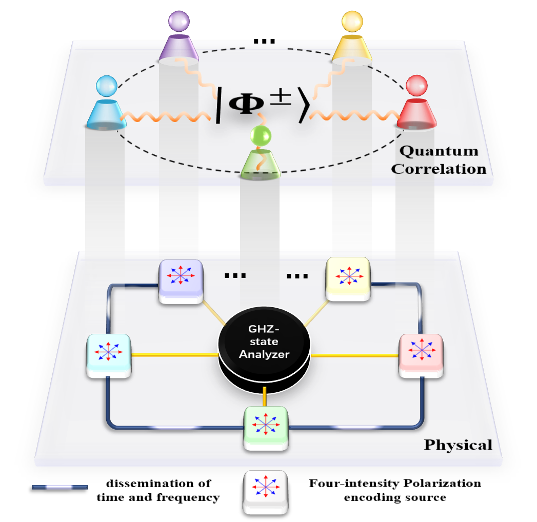
Figure 1: Scheme of polarization encoding measurement-device-independent quantum cryptographic conferencing. In physical layer, multiple users participating in conference randomly prepare polarization-encoded four-intensity pulses with the help of dissemination of time and frequency for synchronization and frequency difference suppression. They send pulses to the GHZ-state analyzer at untrusted detection node for GHZ-state projection measurements. In quantum correlation layer, GHZ-state correlation among all users is generated from successful GHZ-state projection measurement events.

III Experiment

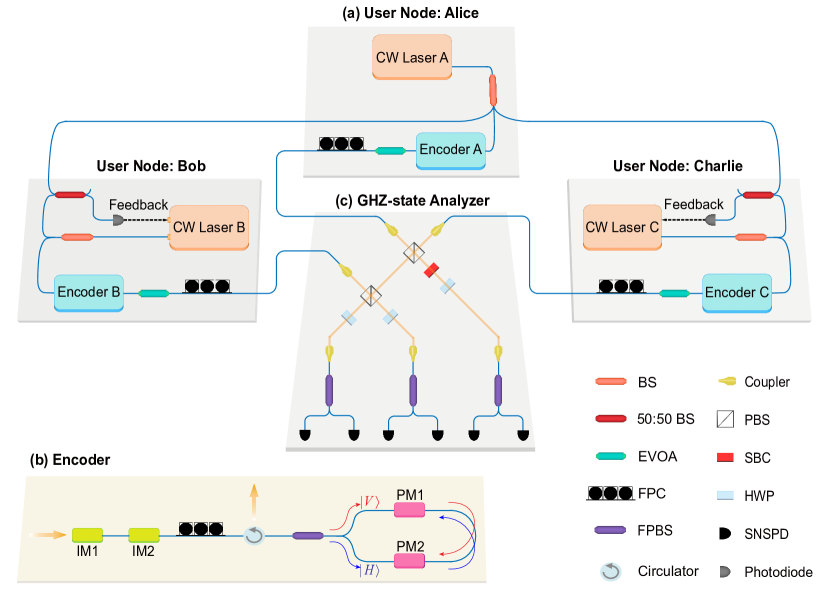
Figure 2: Experimental setup of MDI-QCC. (a) The encoding system to generate polarization qubits for three users, A, B, and C. Each user uses a continuous-wave (CW) laser as the light source. The frequency difference between Alice-Bob and Alice-Charlie is suppressed by means of the feedback control with the beat signal. Decoy states and polarization qubits are realized using an encoder. (b) Detailed structure of the encoder. The four different polarization states are generated by modulating the relative phase between H and V component of incident pulses in a Sagnac loop. (c) GHZ-state analyzer for polarization qubits, see text for details. Abbreviation of the components: BS, beam splitter; EVOA, electrical variable optical attenuator; FPC, fiber polarization controller; IM, intensity modulator; PM, phase modulator; PBS, polarization beam splitter; HWP, half-wave plate; SBC, Soleil-Babinet compensator; SNSPD, superconducting nanowire single-photon detector.

The experimental setup of the MDI-QCC is shown in FIG. 2, which consists of the polarization-encoding optical pulse transmitters held by three users and the GHZ-state analyzer at the untrusted detection node. In the user node, three legitimate users Alice, Bob and Charlie use three independent narrow linewidth CW lasers (A, B, and C) as light sources, whose frequency can be tuned by external voltage controls. Each user splits the light from the laser into two parts, of which 5% is for frequency feedback control and remaining is for encoding. In the frequency feedback control system, Alice interferes her light with Bob’s and Charlie’s on a 50:50 beam splitter for frequency beating respectively. According to the beat signal detected by the photodiode, we feedback onto Bob’s and Charlie’s lasers to regulate the frequency difference between laser A and laser B, as well as that between laser A and laser C within 5 MHz for more than 30 hours.

Another important part of the user node is the encoder. Each encoder can be divided into two parts. In the intensity-encoding part, the first intensity modulator (IM1) chops the CW light into a series of pulses with a repetition frequency of 250 MHz and a duration of about 200 ps. The second intensity modulator (IM2) implements the intensity modulation for the four-intensity decoy-state protocol. The optical pulses then enter the polarization encoder with the initial polarization state $(|H\rangle+|V\rangle)/\sqrt{2}$ [58, 59]. The polarization encoder generates different polarization states by modulating the relative phase between the H and V components of the incident light by the two PMs. By adjusting the relative delay of the electrical signals applied to the PMs, we modulate only the phase of the V component passing clockwise through the loop and keep the phase of H component unchanged. We set the amplitude of the electrical signal on PM1 to $V_{\pi}$ and on the PM2 to $V_{\pi/2}$ so that four relative phases ($0,\pi/2,\pi,3\pi/2$) can be generated to implement polarization encoding. The fidelity of all four polarization states can reach more than 0.99.

After encoding, the electrical variable optical attenuators (EVOAs) are used to attenuate the optical pulses to single-photon level and simulate channel loss. Then the optical pulses are sent into the GHZ-state analyzer. We rotate the polarization state to Z and X basis and compensate the polarization change during propagation by the fiber polarization controllers (FPCs). In our GHZ-state analyzer, we use fiber optical elements including three fiber polarization beam splitters (PBSs) for the part after the half-wave plates (HWPs). For the rest of the analyzer, we use bulk optical elements such as PBSs and HWPs. The angle of the birefringence optical axis of the HWPs on each optical path is set to 22.5^∘. Especially considering the additional phase shift introduced by the PBSs, we add a Soleil-Babinet compensator (SBC) on one of the optical paths in the GHZ-state analyzer for phase compensation [53].

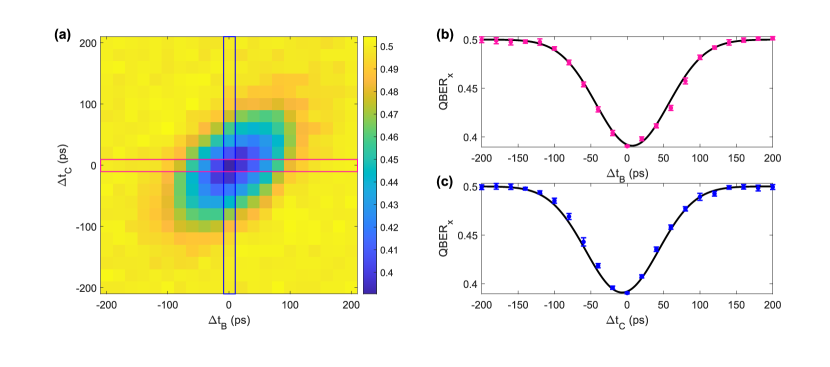
Figure 3: QBER of GHZ-state measurement. (a) $QBER_{X}$ when scanning the relative delay time of Bob and Charlie jointly. (b) and (c) $QBER_{X}$ when scanning the relative delay time of Bob and Charlie in the case of $\Delta t_{C}=0$ (red slice in (a)) and $\Delta t_{B}=0$ (blue slice in (a)) respectively. The black curve is the fitting curve.

To implement the MDI-QCC protocol, we first perform the GHZ-state measurement experiment [60, 61, 62]. When scanning the relative delay time between two users, the three-fold coincidence counts corresponding to the probability of being projected to $|\Phi^{\pm}\rangle$ states shows the dip or peak, which we refer to this generalized Hong-Ou-Mandel (HOM) interference [63] phenomenon as GHZ-HOM interference. The ideal visibility of GHZ-HOM interference with weak coherent state is 25%, resulting in ideal 37.5% $QBER_{X}$ (see Supplemental Materials). We perform the GHZ-HOM experiment with phase-randomized weak coherent state, where three users randomly send X-basis polarization states with the same average photon number. Then we fix the delay time of Alice’s pulses and scan the delay time of Bob’s and Charlie’s pulses. The measurement results are shown in the FIG. 3 and we get $QBER_{X}=39.10\pm 0.09\%$, according to which the average visibility is about $21.80\pm 0.18\%$.

Then in the process of conference key generation, we perform four-intensity MDI-QCC protocol in three different attenuation scenarios. The optimized intensity and probability parameters selected in the experiments are $\mu_{z}=0.100$, $\mu_{x}=0.0281$, $\mu_{y}=0.152$ and the corresponding probabilities $p_{z}=0.33$, $p_{x}=0.51$, $p_{y}=0.09$. We perform the experiments with an overall attenuation of three users of about 14.1 dB, 17.8 dB and 21.5 dB, which includes the total channel loss of three users and the detection efficiency. With an accumulation time of $8\times 10^{4}$ seconds and a total number of pulses of $1.99\times 10^{13}$, we obtain the conference key rates of about 7.54 bps, 1.17 bps and 0.097 bps respectively after decoy-state analysis based on the Chernoff bound method [64], in which we take the failure probability to be $\epsilon=10^{-10}$. The data points and theoretical key rate curves are shown in FIG. 4. We compare the key rate of the three-intensity protocol under the same conditions. The results show that the four-intensity protocol significantly improve the conference key rate and communication distance with finite data size.

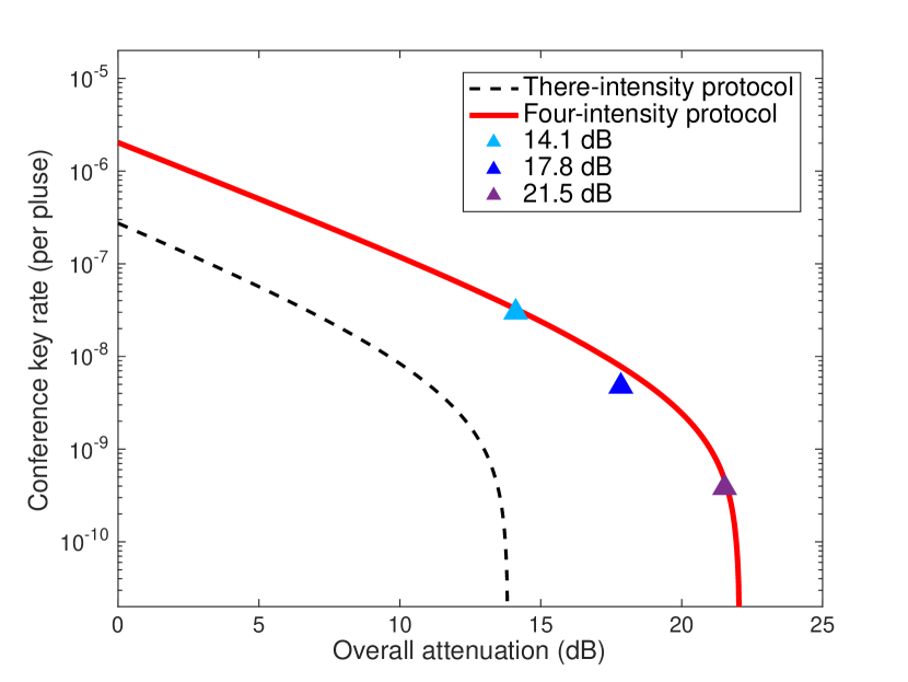
Figure 4: Results of conference key generation. In theoretical calculation, we set the misalignment error $e_{d}=2.25\%$, and take the interference visibility into consideration. We optimize the key rate of the three-intensity protocol under the same condition at the overall attenuation of 13.5 dB. The result shows that the $R_{\text{4-int}}/R_{\text{3-int}}\simeq 110$ at the overall attenuation of 13.5 dB.

IV Discussion

In summary, we experimentally demonstrate the MDI-QCC for the first time by the GHZ-state projection measurement of phase-randomized weak coherent state. Using four-intensity decoy-state MDI-QCC protocol, our experimental work has significantly enhanced the secure conference key rate and communication distance, comparing to the original theoretical proposal. Our work is an important step towards the practical realization of multipartite quantum communication, represented by the transition from two-node, to multi-node experiments within the future quantum internet, Despite these important results, it is noted that the scale of the key rate of our MDI-QCC protocol for N users is $O(\eta^{N})$. With current technology, although it is possible to realize 100-km scale MDI-QCC, covering most applications in metropolitan areas, this scaling may bring limitations to its scalability beyond 100 km. Currently, some single-photon MDI-QCC protocols such as W-state protocols [44, 49] and asynchronous protocols [50, 51] have been proposed, which may overcome this scaling limitations. Based on our work, exploring experimental implementations of single-photon protocols is the next key task in the further research to establish practical MDI-QCC networks.

V Acknowledgment

This research was supported by the National Key Research and Development Program of China (Grants Nos. 2022YFE0137000, 2019YFA0308704), the Natural Science Foundation of Jiangsu Province (Grants Nos. BK20240006, BK20233001), the Leading-Edge Technology Program of Jiangsu Natural Science Foundation (Grant No. BK20192001), the Innovation Program for Quantum Science and Technology (Grants Nos. 2021ZD0300700 and 2021ZD0301500), and the Fundamental Research Funds for the Central Universities (Grants Nos. 2024300324).

Supplemental Materials

S2 S1: Hong-Ou-Mandel interference in GHZ-state measurement

In the MDI-QKD experiments, HOM interference [63] is often used to verify the spectral and temporal indistinguishability of photons from two users. Similarly, in the MDI-QCC experiment, the probability of being projected to GHZ-states shows a peak or dip while scanning the relative delay time. In this section, we theoretically analyze the GHZ-HOM interference with the weak coherent state based on the method given in [65].

S2.1 S1.1: Theory of GHZ-HOM interference with weak coherent states

Assume that the coherent state has the Gaussian temporal and spectral distribution centered at $t_{0}$ and $\omega_{0}$:

$$\begin{split}\left|\Psi\left(t_{0}\right)\right\rangle_{\mathrm{C}}&=\left(\frac{2\Gamma}{\pi}\right)^{\frac{1}{4}}\int_{-\infty}^{\infty}\left|\sqrt{\alpha_{t-t_{0}}}e^{i\theta_{t-t_{0}}}\right\rangle_{C}\mathrm{d}t=\left(\frac{2\Gamma}{\pi}\right)^{\frac{1}{4}}\int_{-\infty}^{\infty}\left|\sqrt{\alpha e^{-2\Gamma(t-t_{0})^{2}}}e^{i\theta^{0}+i\omega_{0}(t-t_{0})}\right\rangle_{C}\mathrm{d}t,\end{split}$$ (S2.1)

in which $\alpha$ is the average photon number; $\theta^{0}$ is the random phase; $\Gamma$ is the linewidth parameter; $\omega_{0}$ and $t_{0}$ are the central frequency and time respectively.

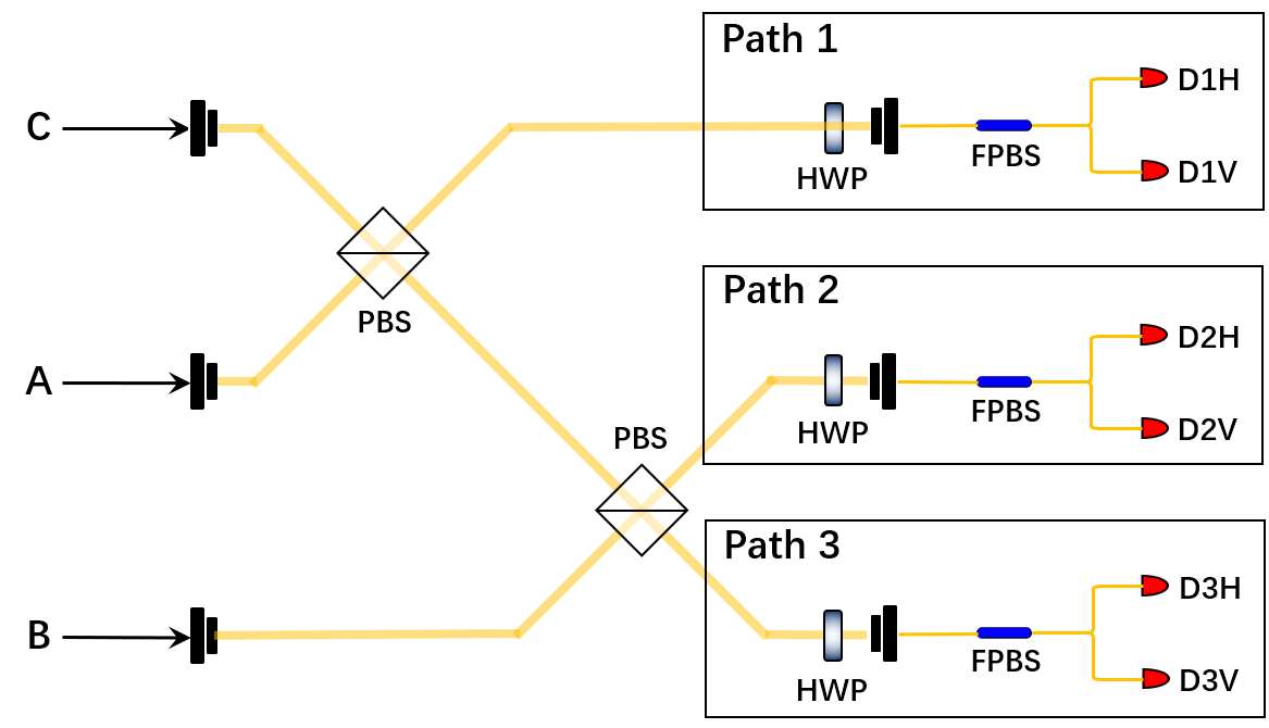
Figure S1: GHZ-state analyzer

Without loss of generality, we assume that three users prepare the polarization state $|+\rangle$ with the average photon number of $\mu,\nu$ and $\kappa$, respectively. i.e. the input states are $\left|\sqrt{\mu}e^{i\varphi_{A}}\right\rangle_{+}\left|\sqrt{\nu}e^{i\varphi_{B}}\right\rangle_{+}\left|\sqrt{\kappa}e^{i\varphi_{C}}\right\rangle_{+}$. Taking into account the temporal distribution, the quantum states arriving at the six detectors after passing through the GHZ-state analyzer are as shown in Figure S1:

$$\left|\psi\right\rangle_{D1H/D1V}=\left({\frac{2\Gamma}{\pi}}\right)^{1/4}\int_{-\infty}^{+\infty}\left|e^{i\varphi_{A}}\left(\frac{\sqrt{\mu_{t-t_{A}}}}{2}\pm\frac{\sqrt{\nu_{t-t_{B}}}}{2}e^{i\varphi_{AB}}\right)\right\rangle\mathrm{d}t,$$ (S2.2)

$$\left|\psi\right\rangle_{D2H/D2V}=\left({\frac{2\Gamma}{\pi}}\right)^{1/4}\int_{-\infty}^{+\infty}\left|e^{i\varphi_{B}}\left(\frac{\sqrt{\nu_{t-t_{B}}}}{2}\pm\frac{\sqrt{\kappa_{t-t_{C}}}}{2}e^{i\varphi_{BC}}\right)\right\rangle\mathrm{d}t,$$ (S2.3)

$$\left|\psi\right\rangle_{D3H/D3V}=\left({\frac{2\Gamma}{\pi}}\right)^{1/4}\int_{-\infty}^{+\infty}\left|e^{i\varphi_{C}}\left(\frac{\sqrt{\kappa_{t-t_{C}}}}{2}\pm\frac{\sqrt{\mu_{t-t_{A}}}}{2}e^{i\varphi_{CA}}\right)\right\rangle\mathrm{d}t,$$ (S2.4)

where the global phase $\varphi_{A,B,C}=\varphi^{0}_{A,B,C}+\omega_{A,B,C}(t-t_{A,B,C})$ are random and $\varphi_{AB,BC,CA}$ are the relative phase between users AB, BC and CA. The phase randomized coherent state with the average photon number $\alpha$ is the mixed state of the photon number state:

$$\rho_{\text{PR}}=\frac{1}{2\pi}\int_{0}^{2\pi}\left|\sqrt{\alpha}e^{i\phi}\right\rangle\left\langle\sqrt{\alpha}e^{i\phi}\right|\mathrm{d}\phi=\sum_{n=0}^{+\infty}\frac{e^{-\alpha}\alpha^{n}}{n!}\left|n\right\rangle\langle n|.$$ (S2.5)

Given that the dark count rate is $p_{d}$ and the detection efficiency is $\eta$, the click probability of a detector is:

$$P=1-\mathrm{e}^{-\alpha}\left(1-p_{d}\right)\sum_{n=0}^{+\infty}\frac{\alpha^{n}}{n!}(1-\eta)^{n}=1-\left(1-p_{d}\right)e^{-\alpha\eta}.$$ (S2.6)

Assuming that $p_{d}=0$ and $\eta=1$, if $\alpha\ll 1$, the click probability above can be approximated as:

$$P\simeq 1-(1-\alpha)=\alpha.$$ (S2.7)

It shows that the click probability of a phase-randomized weak coherent state is approximately equal to its average photon number. According to the eq. (S2.7), for example, the click probability of a single detector D1H or D1V can be expanded as:

$$\begin{split}\mathrm{P}_{D1H/D1V}=\sqrt{\frac{\Gamma}{8\pi}}&\int_{-\infty}^{+\infty}\left[\mu e^{-2\Gamma\left(t-t_{A}\right)^{2}}+\nu e^{-2\Gamma\left(t-t_{B}\right)^{2}}\pm 2\sqrt{\mu\nu}e^{-2\Gamma\left(t-\frac{t_{A}+t_{B}}{2}\right)^{2}-\frac{\Gamma\Delta t^{2}_{AB}}{2}}\cos\left(\Delta\omega_{AB}t+\phi_{AB}\right)\right]\mathrm{d}t,\end{split}$$ (S2.8)

where $\phi_{AB}=\Delta\varphi^{0}_{AB}+\omega_{A}t_{A}-\omega_{B}t_{B}$ is the random phase. In the same way we can obtain the click probabilities of the remaining four detectors. After calculating the integration, we have:

$$\mathrm{P}_{D1H/D1V}=\frac{1}{4}(\mu+\nu)\pm\frac{1}{2}\sqrt{\mu\nu}e^{-\frac{\Gamma\Delta t^{2}_{AB}}{2}-\frac{\Delta\omega_{AB}^{2}}{8\Gamma}}\cos\left(\Delta\phi_{AB}\right),$$ (S2.9)

$$\mathrm{P}_{D2H/D2V}=\frac{1}{4}(\kappa+\nu)\pm\frac{1}{2}\sqrt{\kappa\nu}e^{-\frac{\Gamma\Delta t^{2}_{BC}}{2}-\frac{\Delta\omega_{BC}^{2}}{8\Gamma}}\cos\left(\Delta\phi_{BC}\right),$$ (S2.10)

$$\mathrm{P}_{D3H/D3V}=\frac{1}{4}(\mu+\kappa)\pm\frac{1}{2}\sqrt{\mu\kappa}e^{-\frac{\Gamma\Delta t^{2}_{CA}}{2}-\frac{\Delta\omega_{CA}^{2}}{8\Gamma}}\cos\left(\Delta\phi_{CA}\right).$$ (S2.11)

We assume that $\mu=\nu=\kappa$ and the frequency difference between two users is sufficiently small, i.e. $\Delta\omega^{2}/8\Gamma\simeq 0$. Then the 3-fold coincidence count rate is the product of the click probabilities of the corresponding detectors, i.e. the probabilities of being projected to the $|\Phi^{+}\rangle$ state and the $|\Phi^{-}\rangle$ state are:

$$P_{|\Phi^{+}\rangle}(\phi_{AB},\phi_{CA})=P_{D1H}P_{D2H}P_{D3H}+P_{D1H}P_{D2V}P_{D3V}+P_{D1V}P_{D2H}P_{D3V}+P_{D1V}P_{D2V}P_{D3H},$$ (S2.12)

$$P_{|\Phi^{-}\rangle}(\phi_{AB},\phi_{CA})=P_{D1V}P_{D2V}P_{D3V}+P_{D1V}P_{D2H}P_{D3H}+P_{D1H}P_{D2V}P_{D3H}+P_{D1H}P_{D2H}P_{D3V}.$$ (S2.13)

Considering that the random phase is uniformly distributed on $[0,2\pi]$, the final result can be obtained by taking the mean of eq. (S2.12) and eq. (S2.13):

$$\begin{split}P_{|\Phi^{+}\rangle}&=\frac{1}{4\pi^{2}}\int_{0}^{2\pi}\mathrm{d}\phi_{AB}\int_{0}^{2\pi}\mathrm{d}\phi_{CA}{P_{|\Phi^{+}\rangle}(\phi_{AB},\phi_{CA})}=\frac{\mu^{3}}{2}\left[1+{\color[rgb]{0,0,0}\frac{1}{4}}e^{-\frac{\Gamma}{2}\left(\Delta t_{AB}^{2}+\Delta t_{AC}^{2}+\Delta t_{BC}^{2}\right)}\right],\end{split}$$ (S2.14)

$$\begin{split}P_{|\Phi^{-}\rangle}&=\frac{1}{4\pi^{2}}\int_{0}^{2\pi}\mathrm{d}\phi_{AB}\int_{0}^{2\pi}\mathrm{d}\phi_{CA}{P_{|\Phi^{-}\rangle}(\phi_{AB},\phi_{CA})}=\frac{\mu^{3}}{2}\left[1-{\color[rgb]{0,0,0}\frac{1}{4}}e^{-\frac{\Gamma}{2}\left(\Delta t_{AB}^{2}+\Delta t_{AC}^{2}+\Delta t_{BC}^{2}\right)}\right].\end{split}$$ (S2.15)

From the two equations above, we can conclude that the theoretical visibility for coincidence dip and peak of GHZ-HOM interference are as follows:

$$V_{\text{dip}}=\left(\overline{P}-\underline{P}\right)/{\overline{P}}=0.25,$$ (S2.16)

$$V_{\text{peak}}=\left(\overline{P}-\underline{P}\right)/{\underline{P}}=0.25,$$ (S2.17)

where $\overline{P}$ and $\underline{P}$ is the supremum and infimum of the projection probability. Generally, in the case of $V_{\text{dip}}=V_{\text{peak}}=V$, the $QBER_{X}$ is:

$$QBER_{X}=\frac{P_{|\Phi^{-}\rangle}}{P_{|\Phi^{+}\rangle}+P_{|\Phi^{-}\rangle}}=\frac{1}{2}\left[1-Ve^{-\frac{\Gamma}{2}\left(\Delta t_{AB}^{2}+\Delta t_{AC}^{2}+\Delta t_{BC}^{2}\right)}\right].$$ (S2.18)

When the light pulses coincide exactly in the time domain, i.e. $\Delta t_{AB}=\Delta t_{AC}=\Delta t_{BC}=0$, we have $QBER_{X}=(1-V)/2$, which means that $QBER_{X}=0.375$ when $V=0.25$.

S2.2 S1.2: Experiment of GHZ-HOM interference

S2.2.1 Two-photon HOM interference

In order to align the optical pulses of the three users in the time domain, we first perform the two-photon HOM interference experiment. The results are shown in the figure below:

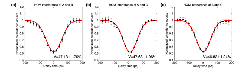
Figure S2: Two-photon HOM interference. (a) user A and user B; (b) user A and user C; (c) user B and user C. The black points are measurement data; the red lines are the fitting curves.

S2.2.2 Compensation of the phase shift

We assume that the additional relative phase shift introduced by the polarization beam splitters on the $|V\rangle$ component for users A, B and C is $\gamma_{1},\gamma_{2}$ and $\gamma_{3}$ respectively. The click probabilities of six detectors can be modified as follows:

$$\mathrm{P}_{D1H/D1V}=\frac{1}{4}(\mu+\nu)\pm\frac{1}{2}\sqrt{\mu\nu}e^{-\frac{\Gamma\Delta t^{2}_{AB}}{2}-\frac{\Delta\omega_{AB}^{2}}{8\Gamma}}\cos\left(\Delta\phi_{AB}+\gamma_{1}\right),$$ (S2.19)

$$\mathrm{P}_{D2H/D2V}=\frac{1}{4}(\kappa+\nu)\pm\frac{1}{2}\sqrt{\kappa\nu}e^{-\frac{\Gamma\Delta t^{2}_{BC}}{2}-\frac{\Delta\omega_{BC}^{2}}{8\Gamma}}\cos\left(\Delta\phi_{BC}+\gamma_{2}\right),$$ (S2.20)

$$\mathrm{P}_{D3H/D3V}=\frac{1}{4}(\mu+\kappa)\pm\frac{1}{2}\sqrt{\mu\kappa}e^{-\frac{\Gamma\Delta t^{2}_{CA}}{2}-\frac{\Delta\omega_{CA}^{2}}{8\Gamma}}\cos\left(\Delta\phi_{CA}+\gamma_{3}\right),$$ (S2.21)

Repeating the same calculation as above, we can get the visibility:

$$V=\frac{1}{4}\cos(\gamma_{1}+\gamma_{2}+\gamma_{3}).$$ (S2.22)

To eliminate the effect of additional phase on the interference, we add a Soleil-Babinet Compensator (SBC) in the optical path to adjust $\gamma_{1}$ to satisfy the condition $\gamma_{1}+\gamma_{2}+\gamma_{3}=2k\pi(k\in\mathbb{Z})$. In the experiment, three users randomly send two polarization states in X-basis with the equal probability. After aligning the pulses in the time and frequency domain, we scan the distance of the SBC from 0 to 20 mm in a 1mm steps. Each data point corresponds to a measurement lasting 50 s with coincidence time window of about 500 ps. The result is shown in Figure S3:

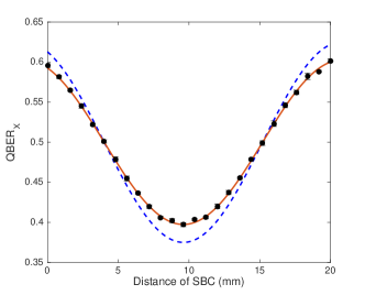
Figure S3: ${QBER}_{{X}}$ versus the distance of SBC. The black points are measurement data; the red line is the fitting curve; the blue dashed line is the theoretical curve. Since the compensation phase of the SBC is linearly related to the distance, $QBER_{X}$ is cosine-related to $\gamma_{1}$, which is consistent with the theoretical result.

S2.2.3 Results of GHZ-HOM interference

After adjusting the SBC to compensate phase shift, we scan the relative delay time between user AB and AC from -200 ps to 200 ps in the 20 ps steps. Each data point corresponds to a measurement lasting 60 seconds with coincidence time window of about 500 ps. The original 3-fold coincidence counts of the GHZ-HOM interference with different input states are shown in Figure S4 and Figure S5.

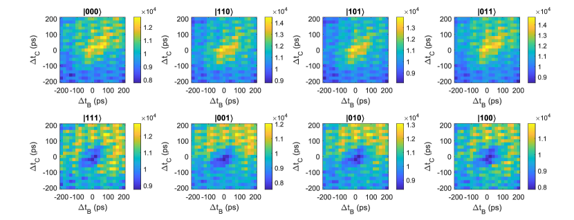
Figure S4: Original coincidence counts projected to $|\Phi^{+}\rangle$ of eight states in X-basis

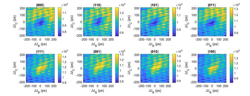
Figure S5: Original coincidence counts projected to $|\Phi^{-}\rangle$ of eight states in X-basis

Considering the overall fluctuation while scanning the delay time, we calculate the proportional coincidence counts as:

$$\bar{N}^{|\Phi^{+/-}\rangle}_{|\psi\rangle}=\frac{1}{C_{\text{fit}}}\frac{16N^{|\Phi^{+/-}\rangle}_{|\psi\rangle}}{N_{\text{total}}},$$ (S2.23)

where $N^{|\Phi^{+/-}\rangle}_{|\psi\rangle}$ is the coincidence counts projected onto $|\Phi^{+}\rangle$ or $|\Phi^{-}\rangle$ state with the input state $|\psi\rangle$; $N_{\text{total}}$ is the total coincidence counts of all input states; and the $C_{\text{fit}}$ is the normalization constant obtained by the fitting results.

The processed coincidence counts and $QBER_{X}$ as a function of $\Delta t_{B}$ and $\Delta t_{C}$ are shown in Figure S6, Figure S7 and Figure S8. The visibilities are obtained by fitting the $QBER_{X}$ data based on the theoretical equation eq. (1.18) and the results are shown in Table S1.

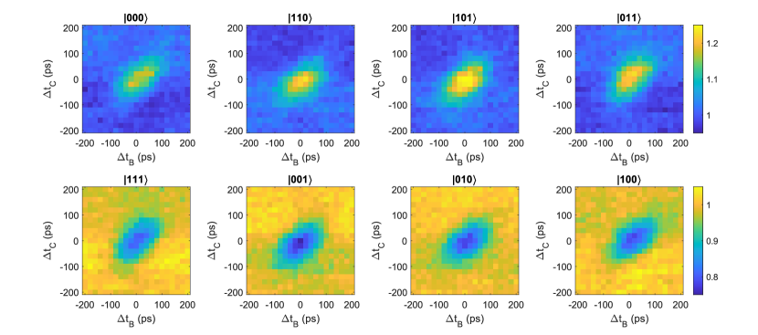
Figure S6: Processed coincidence counts projected to $|\Phi^{+}\rangle$ of eight input states in X-basis

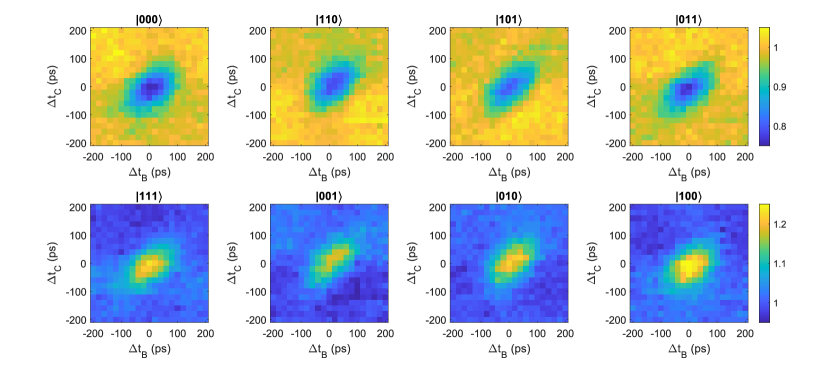
Figure S7: Processed coincidence counts projected to $|\Phi^{-}\rangle$ of eight input states in X-basis

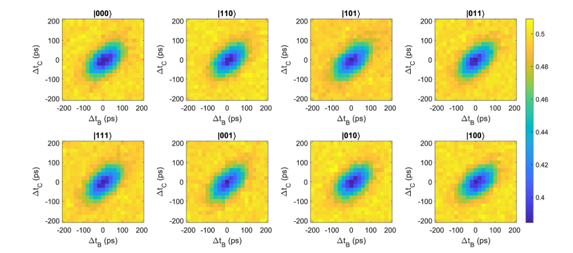
Figure S8: $QBER_{X}$ of eight input states in X-basis

Input state	Visibility ($\%$)	$QBER_{X}$ ($\%$)
$|000\rangle$	$21.72\pm 0.33$	$39.14\pm 0.17$
$|001\rangle$	$21.20\pm 0.35$	$39.40\pm 0.18$
$|010\rangle$	$22.26\pm 0.30$	$38.87\pm 0.15$
$|011\rangle$	$21.87\pm 0.33$	$39.07\pm 0.17$
$|100\rangle$	$22.83\pm 0.35$	$38.59\pm 0.18$
$|101\rangle$	$22.24\pm 0.36$	$38.88\pm 0.18$
$|110\rangle$	$21.47\pm 0.29$	$39.27\pm 0.15$
$|111\rangle$	$21.09\pm 0.31$	$39.46\pm 0.16$

Table S1: Visibility of GHZ-HOM interference and $QBER_{X}$ of eight input states

S3 S2: Frequency and polarization stability

The overall stability of the system is critical due to the long period of time required to accumulate data in the experiment. On the one hand, the frequency difference between the independent lasers can be suppressed to less than 5 MHz by feedback control and can be kept stable within $10^{5}$ seconds as shown in Figure S9. On the other hand, the $QBER_{X}$ and $QBER_{Z}$ of the system can be kept at a low level within about 8 hours, indicating that our polarization encoders and the GHZ-state analyzer also can be kept stable over a relatively long time as shown in Figure S10. Besides, the degree of polarization (DOP) and fidelity of four states prepared by three users are shown in Table S2. In the experiment, we check the $QBER_{X}$ and $QBER_{Z}$ every 1000 seconds and adjust the system if the error rate is too high to generate the secure key. We adjusted the system on average $1\sim 3$ times during the measurement time of about 23 hours.

	$|D\rangle$		$|A\rangle$		$|H\rangle$		$|V\rangle$
	$\phi_{1}=0$	$\phi_{2}=0$	$\phi_{1}=\pi$	$\phi_{2}=0$	$\phi_{1}=0$	$\phi_{2}=\frac{\pi}{2}$	$\phi_{1}=\pi$	$\phi_{2}=\frac{\pi}{2}$
	$V_{1}=0$	$V_{2}=0$	$V_{1}=V_{\pi}$	$V_{2}=0$	$V_{1}=0$	$V_{2}=V_{\frac{\pi}{2}}$	$V_{1}=V_{\pi}$	$V_{2}=V_{\frac{\pi}{2}}$
	DOP	Fidelity	DOP	Fidelity	DOP	Fidelity	DOP	Fidelity
user A	$1.000(8)$	$1.000(3)$	$0.987(3)$	$0.996(1)$	$0.980(7)$	$0.995(2)$	$0.991(2)$	$0.997(1)$
user B	$1.000(3)$	$1.000(1)$	$0.996(3)$	$0.999(1)$	$0.967(6)$	$0.992(2)$	$0.986(2)$	$0.996(1)$
user C	$1.000(2)$	$1.000(1)$	$0.995(3)$	$0.998(1)$	$0.969(7)$	$0.992(2)$	$0.995(2)$	$0.998(1)$

Table S2: Degree of polarization (DOP) and fidelity of four polarization states output by the encoder. We remark that in the experiment we set the polarization state $|D\rangle$ as reference

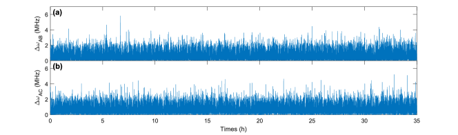
Figure S9: Frequency difference between two users within $10^{5}$s. (a) $|\Delta\omega_{AB}|$, (b) $|\Delta\omega_{AC}|$ .

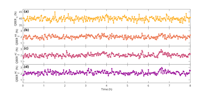
Figure S10: QBERs within 8 hours. For X-basis pulse pairs, (a) $QBER_{X}=39.78\pm 1.40\%$. For Z-basis pulse pairs, (b) $e_{Z}^{AB}=2.00\pm 0.24\%$, (c) $e_{Z}^{AC}=2.02\pm 0.24\%$, (d) $e_{Z}^{BC}=2.14\pm 0.25\%$

S4 S3: Conference key rate of four-intensity MDI-QCC protocol

In this section, we derive the formulas for the decoy-state analysis of the four-intensity MDI-QCC protocol based on the method in [54]. Then we perform numerical simulations for the four-intensity protocol and the original three-intensity protocol. The results show that the four-intensity protocol significantly improves the key rate and the communication distance of the polarization-encoding MDI-QCC with finite data size.

S3.1 S3.1: Decoy state analysis

In the four-intensity decoy-state protocol, each user uses four light sources with different intensities: the signal source $z$ with the average photon number of $\mu_{z}$ is encoded only on the Z-basis; the decoy sources $x$, $y$ with the average photon number of $\mu_{x}$, $\mu_{y}$ respectively are encoded on the X-basis, where $\mu_{y}>\mu_{x}$; the vacuum source with $\mu_{o}=0$. The density matrix of phase-randomized weak coherent state pulses generated by three non-vacuum light sources can be expressed as:

$$\rho_{z}=\sum_{n=0}^{\infty}{u_{n}^{z}|n\rangle\langle n|}\quad\rho_{x}=\sum_{n=0}^{\infty}{u_{n}^{x}|n\rangle\langle n|}\quad\rho_{y}=\sum_{n=0}^{\infty}{u_{n}^{y}|n\rangle\langle n|}\quad u=a,b,c.$$ (S3.1)

In the calculation below we use $\langle\cdot\rangle$ to denote the expectation values. When three users use the $x$ source or $y$ source, the gains can be expressed as the sum of the yields of the components with different photon numbers:

$$\langle Q_{xxx}\rangle=\sum_{i,j,k=0}{a^{x}_{i}b^{x}_{j}c^{x}_{k}\langle Y_{ijk}\rangle},$$ (S3.2)

$$\langle Q_{yyy}\rangle=\sum_{i,j,k=0}{a^{y}_{i}b^{y}_{j}c^{y}_{k}\langle Y_{ijk}\rangle}.$$ (S3.3)

Then the gains including vacuum sources are:

$$\begin{split}&\langle Q_{sso}\rangle=\sum_{i,j=0}{a^{s}_{i}b^{s}_{j}\langle Y_{ij0}\rangle},\quad\langle Q_{sos}\rangle=\sum_{i,k=0}{a^{s}_{i}c^{s}_{k}\langle Y_{i0k}\rangle},\quad\langle Q_{oss}\rangle=\sum_{j,k=0}{b^{s}_{j}c^{s}_{k}\langle Y_{0jk}\rangle},\end{split}$$ (S3.4)

$$\begin{split}&\langle Q_{soo}\rangle=\sum_{i=0}{a^{s}_{i}\langle Y_{i00}\rangle},\quad\langle Q_{oso}\rangle=\sum_{j=0}{b_{j}^{s}\langle Y_{0j0}\rangle},\quad\langle Q_{oos}\rangle=\sum_{k=0}{c^{s}_{k}\langle Y_{00k}\rangle},\end{split}$$ (S3.5)

$$\langle Q_{ooo}\rangle=\langle Y_{000}\rangle.$$ (S3.6)

in which $s=x,y$. Combining the above equations, we can get the gain excluding the part that includes the vacuum component:

$$\widetilde{Q}_{xxx}=\langle Q_{xxx}\rangle-\langle\mathcal{H}_{xxx}\rangle=\sum_{i,j,k=1}{a^{x}_{i}b^{x}_{j}c^{x}_{k}\langle Y_{ijk}\rangle}=a^{x}_{1}b^{x}_{1}c^{x}_{1}\langle Y_{111}\rangle+a^{x}_{1}b^{x}_{2}c^{x}_{1}\langle Y_{121}\rangle+\cdots,$$ (S3.7)

$$\widetilde{Q}_{yyy}=\langle Q_{yyy}\rangle-\langle\mathcal{H}_{yyy}\rangle=\sum_{i,j,k=1}{a^{y}_{i}b^{y}_{j}c^{y}_{k}\langle Y_{ijk}\rangle}=a^{y}_{1}b^{y}_{1}c^{y}_{1}\langle Y_{111}\rangle+a^{y}_{1}b^{y}_{2}c^{y}_{1}\langle Y_{121}\rangle+\cdots,$$ (S3.8)

where the excluded parts are:

$$\begin{split}\langle\mathcal{H}_{xxx}\rangle=a^{x}_{0}\langle Q_{oxx}\rangle&+b^{x}_{0}\langle Q_{xox}\rangle+c^{x}_{0}\langle Q_{xxo}\rangle\\ &-a^{x}_{0}b^{x}_{0}\langle Q_{oox}\rangle-a^{x}_{0}c^{x}_{0}\langle Q_{oxo}\rangle-b^{x}_{0}c^{x}_{0}\langle Q_{xoo}\rangle+a^{x}_{0}b^{x}_{0}c^{x}_{0}\langle Q_{ooo}\rangle,\end{split}$$ (S3.9)

$$\begin{split}\langle\mathcal{H}_{yyy}\rangle=a^{y}_{0}\langle Q_{oyy}\rangle&+b^{y}_{0}\langle Q_{yoy}\rangle+c^{y}_{0}\langle Q_{yyo}\rangle\\ &-a^{y}_{0}b^{y}_{0}\langle Q_{ooy}\rangle-a^{y}_{0}c^{y}_{0}\langle Q_{oyo}\rangle-b^{y}_{0}c^{y}_{0}\langle Q_{yoo}\rangle+a^{y}_{0}b^{y}_{0}c^{y}_{0}\langle Q_{ooo}\rangle.\end{split}$$ (S3.10)

To estimate the yield of the single-photon component, we need to eliminate the terms $\langle Y_{211}\rangle$, $\langle Y_{121}\rangle$, and $\langle Y_{112}\rangle$ from the above two formulas. We assume that three users use the same light sources in the protocol, i.e. $a_{n}^{s}=b_{n}^{s}=c_{n}^{s}$. These terms can be eliminated as:

$$\begin{split}a^{y}_{1}b^{y}_{2}c^{y}_{1}\widetilde{Q}_{xxx}-a^{x}_{1}b^{x}_{2}c^{x}_{1}\widetilde{Q}_{yyy}&=\left[a_{1}^{x}a_{1}^{y}c_{1}^{x}c_{1}^{y}\left(b_{1}^{x}b_{2}^{y}-b_{2}^{x}b_{1}^{y}\right)\right]\langle Y_{111}\rangle\\ &+\sum_{\begin{subarray}{c}m+n+p\geq 5\\ m\geq 1,n\geq 1,p\geq 1\end{subarray}}{\left(a_{1}^{y}b_{2}^{y}c_{1}^{y}a_{m}^{x}b_{n}^{x}c_{p}^{x}-a_{1}^{x}b_{2}^{x}c_{1}^{x}a_{m}^{y}b_{n}^{y}c_{p}^{y}\right)\langle Y_{mnp}\rangle}.\end{split}$$ (S3.11)

For the weak coherent state, we have:

$$\frac{u_{k}^{y}}{u_{k}^{x}}=\frac{e^{-\mu_{y}}\mu_{y}^{k}/k!}{e^{-\mu_{x}}\mu_{x}^{k}/k!}=e^{\mu_{x}-\mu_{y}}\left(\frac{\mu_{y}}{\mu_{x}}\right)^{k}.$$ (S3.12)

Since $\mu_{x}<\mu_{y}$, the coefficient of the $\langle Y_{mnp}\rangle$ term in the above formula can be rewritten as:

$$\left(a_{1}^{y}b_{2}^{y}c_{1}^{y}a_{m}^{x}b_{n}^{x}c_{p}^{x}-a_{1}^{x}b_{2}^{x}c_{1}^{x}a_{m}^{y}b_{n}^{y}c_{p}^{y}\right)=a_{1}^{x}b_{2}^{x}c_{1}^{x}a_{m}^{x}b_{n}^{x}c_{p}^{x}\left(\frac{a_{1}^{y}}{a_{1}^{x}}\frac{b_{2}^{y}}{b_{2}^{x}}\frac{c_{1}^{y}}{c_{1}^{x}}-\frac{a_{m}^{y}}{a_{m}^{x}}\frac{b_{n}^{y}}{b_{n}^{x}}\frac{c_{p}^{y}}{c_{p}^{x}}\right).$$ (S3.13)

According to the formulas above, we have:

$$\left(\frac{a_{1}^{y}}{a_{1}^{x}}\frac{b_{2}^{y}}{b_{2}^{x}}\frac{c_{1}^{y}}{c_{1}^{x}}-\frac{a_{m}^{y}}{a_{m}^{x}}\frac{b_{n}^{y}}{b_{n}^{x}}\frac{c_{p}^{y}}{c_{p}^{x}}\right)=e^{3(\mu_{x}-\mu_{y})}\left[\left(\frac{\mu_{y}}{\mu_{x}}\right)^{4}-\left(\frac{\mu_{y}}{\mu_{x}}\right)^{m+n+p}\right]\leq e^{3(\mu_{x}-\mu_{y})}\left(\frac{\mu_{y}}{\mu_{x}}\right)^{4}\left[1-\left(\frac{\mu_{y}}{\mu_{x}}\right)\right]<0.$$ (S3.14)

Thus the coefficients of $\langle Y_{mnp}\rangle$ are negative. Then we can obtain the lower bound of the single-photon yield of X-basis as:

$$\langle Y_{111}^{X}\rangle\geq\langle Y_{111}^{X}\rangle^{L}(\mathcal{H})=\frac{a^{y}_{1}b^{y}_{2}c^{y}_{1}\widetilde{Q}_{xxx}-a^{x}_{1}b^{x}_{2}c^{x}_{1}\widetilde{Q}_{yyy}}{a_{1}^{x}a_{1}^{y}c_{1}^{x}c_{1}^{y}\left(b_{1}^{x}b_{2}^{y}-b_{2}^{x}b_{1}^{y}\right)}=\frac{S^{L}_{+}-S^{U}_{-}-e^{-3\mu_{y}}\mu_{y}^{4}\mathcal{H}}{e^{-3\mu_{x}-3\mu_{y}}\left(\mu_{x}^{3}\mu_{y}^{4}-\mu_{x}^{4}\mu_{y}^{3}\right)},$$ (S3.15)

where

$$\mathcal{H}=\mathcal{H}_{xxx},$$ (S3.16)

$$\begin{split}{S}_{+}=e^{-3\mu_{y}}\mu_{y}^{4}\langle Q_{xxx}\rangle&+e^{-3\mu_{x}}\mu_{x}^{4}\left[e^{-3\mu_{y}}\langle Q_{ooo}\rangle+\right.\left.e^{-\mu_{y}}\left(\langle Q_{oyy}\rangle+\langle Q_{yoy}\rangle+\langle Q_{yyo}\rangle\right)\right],\end{split}$$ (S3.17)

$${S}_{-}=e^{-3\mu_{x}}\mu_{x}^{4}\left[\langle Q_{yyy}\rangle+e^{-2\mu_{y}}\left(\langle Q_{yoo}\rangle+\langle Q_{oyo}\rangle+\langle Q_{ooy}\rangle\right)\right].$$ (S3.18)

On the other hand, we can also use the same method to estimate the single-photon phase error rate with the bit error rate of $x$-source pulses. Considering that the polarization state of the vacuum state can be randomly assigned to the $|+\rangle$ state or the $|-\rangle$ state with equal probability in the statistical process, the single-photon bit error rate of the X-basis pulses can be estimated as follows:

$$\left\langle E_{xxx}Q_{xxx}\right\rangle-\frac{1}{2}\langle\mathcal{H}_{xxx}\rangle=\sum_{j,k,l\geq 1}a_{j}^{x}b_{k}^{x}c_{l}^{x}\left\langle e_{jkl}Y_{jkl}\right\rangle\geqslant a_{1}^{x}b_{1}^{x}c^{x}_{1}\left\langle e_{111}Y_{111}\right\rangle.$$ (S3.19)

The upper bound of the single-photon quantum bit error rate of the X-basis pulses is:

$$\langle e_{111}^{BX}\rangle\leq\langle e_{111}^{BX}\rangle^{U}(\mathcal{H})=\frac{\left\langle E_{xxx}Q_{xxx}\right\rangle^{U}-\langle\mathcal{H}\rangle/2}{\mu_{x}^{3}e^{-3\mu_{x}}\langle Y_{111}\rangle^{L}}.$$ (S3.20)

Finally, considering that the expectation values satisfy $\langle Y_{111}^{X}\rangle=\langle Y_{111}^{Z}\rangle$ and $\langle e_{111}^{BX}\rangle=\langle e_{111}^{PZ}\rangle$, the key rate of the MDI-QCC protocol can be represented as the function of $\mathcal{H}$:

$$R(\mathcal{H})=p_{z}^{3}\left\{\mu_{z}^{3}e^{-3\mu_{z}}Y_{111}^{Z}\left[1-H\left(e_{111}^{PZ}\right)\right]-Q_{zzz}f\text{max}\left[H\left(e_{Z}^{AB}\right),H\left(e_{Z}^{AC}\right),H\left(e_{Z}^{BC}\right)\right]\right\}.$$ (S3.21)

S3.2 S3.2: Finite key size analysis with Chernoff bound

In the experiment, the number of pulses is finite, hence we need to take the statistical fluctuation into consideration. To calculate the secure key rate, we need to estimate the real value of the single-photon yield $Y_{111}^{Z}$ and the phase error rate $e_{111}^{PZ}$ of the Z-basis pulses, which cannot be measured directly in the experiment. In our calculation, according to the formulas in Section 3.1, we first estimate the expectation values $\langle Y_{111}^{X}\rangle^{L}$ and $\langle e_{111}^{BX}\rangle^{U}$ with the Chernoff bound method [64, 66, 67] and the joint constraints. Since the expectation values satisfy $\langle Y_{111}^{X}\rangle=\langle Y_{111}^{Z}\rangle$ and $\langle e_{111}^{BX}\rangle=\langle e_{111}^{PZ}\rangle$, we can use the Chernoff bound again to obtain the real values.

S3.2.1 Chernoff bound

Let $X_{1},X_{2},\dots,X_{n}$ be the measurement results of $n$ independent random events. If the measurement is successful, record it as 1, otherwise, record it as 0. Let $\chi=\sum_{i=1}^{n}{X_{i}}$ be the sum of the measurement results and $\langle\chi\rangle=\mathbb{E}(\chi)$ be the expected value of $\chi$.

• From $\chi$ to $\langle\chi\rangle$. Given the measurement result $\chi$ and the failure probability $\varepsilon$, the confidence interval of expected value satisfying $\text{Pr}\{\langle\chi\rangle>\mathbb{E}^{L}(\chi)\}=\text{Pr}\{\langle\chi\rangle<\mathbb{E}^{U}(\chi)\}\leq\varepsilon/2$ can be evaluated as:

  $$\langle\chi\rangle^{L}=\mathbb{E}^{L}(\chi)=\frac{\chi}{1+\delta^{L}},\quad\langle\chi\rangle^{U}=\mathbb{E}^{U}(\chi)=\frac{\chi}{1-\delta^{U}},$$ (S3.22)

  where $\delta^{L}$ and $\delta^{U}$ can be obtained by solving the equations below:

  $${\left[\frac{e^{\delta^{L}}}{\left(1+\delta^{L}\right)^{1+\delta^{L}}}\right]^{\chi/\left(1+\delta^{L}\right)}=\frac{1}{2}\varepsilon},\quad{\left[\frac{e^{-\delta^{U}}}{\left(1-\delta^{U}\right)^{1-\delta^{U}}}\right]^{\chi/\left(1-\delta^{U}\right)}=\frac{1}{2}\varepsilon}.$$ (S3.23)

  Let $b=-\ln{(\varepsilon/2)}$, if $\chi\geq 6b$, we use approximation [66]:

  $$\delta^{L}=\delta^{U}=\frac{3b+\sqrt{8b\chi+b^{2}}}{2(\chi-b)}.$$ (S3.24)

  If the measurement result is 0, we have:

  $$\mathbb{E}^{L}(\chi)=0,\quad\mathbb{E}^{U}(\chi)=b.$$ (S3.25)

• From $\langle\chi\rangle$ to $\chi$. Given the expected value $\langle\chi\rangle$ the confidence interval of the real value satisfying $\text{Pr}\{\chi\in[\chi^{L},\chi^{U}]\}\geq 1-\varepsilon$ can be evaluated as:

  $$\chi^{L}=\mathbb{O}^{L}(\langle\chi\rangle)=(1-\delta^{\prime U})\langle\chi\rangle,\quad\chi^{U}=\mathbb{O}^{U}(\langle\chi\rangle)=(1+\delta^{\prime L})\langle\chi\rangle,$$ (S3.26)

  where $\delta^{L}$ and $\delta^{U}$ can be samely obtained by solving the equations below:

  $${\left[\frac{e^{\delta^{\prime L}}}{\left(1+\delta^{\prime L}\right)^{1+\delta^{\prime L}}}\right]^{\langle\chi\rangle}=\frac{1}{2}\varepsilon},\quad{\left[\frac{e^{-\delta^{\prime U}}}{\left(1-\delta^{\prime U}\right)^{1-\delta^{\prime U}}}\right]^{\langle\chi\rangle}=\frac{1}{2}\varepsilon}.$$ (S3.27)

  According to the results in [66], in the calculation we use the formula:

  $$\delta^{\prime L}=\delta^{\prime U}=\frac{b+\sqrt{b^{2}+8b\langle\chi\rangle}}{2\langle\chi\rangle}.$$ (S3.28)

  where $b=-\ln{(\varepsilon/2)}$.

S3.2.2 Joint constraints

In computing $S_{+}$ and $S_{-}$, similar to the method in [54], we introduce a set of joint constraints and perform linear programming to find the minimum and maximum values, respectively. In the inequalities below we denote $n$ as measurement values and $N$ as the number of pulses. 26 inequalities are introduced to calculate the minimum value of $S_{+}$.

The joint constraints for all 5 variables are:

$$N_{xxx}\langle Q_{xxx}\rangle+N_{oyy}\langle Q_{oyy}\rangle+N_{yoy}\langle Q_{yoy}\rangle+N_{yyo}\langle Q_{yyo}\rangle+N_{ooo}\langle Q_{ooo}\rangle\geq\mathbb{E}^{L}(n_{xxx}+n_{oyy}+n_{yoy}+n_{yyo}+n_{ooo}).$$ (S3.29)

The joint constraints for 4 variables are:

$$N_{oyy}\langle Q_{oyy}\rangle+N_{yoy}\langle Q_{yoy}\rangle+N_{yyo}\langle Q_{yyo}\rangle+N_{ooo}\langle Q_{ooo}\rangle\geq\mathbb{E}^{L}(n_{oyy}+n_{yoy}+n_{yyo}+n_{ooo}),$$ (S3.30)

$$N_{xxx}\langle Q_{xxx}\rangle+N_{yoy}\langle Q_{yoy}\rangle+N_{yyo}\langle Q_{yyo}\rangle+N_{ooo}\langle Q_{ooo}\rangle\geq\mathbb{E}^{L}(n_{xxx}+n_{yoy}+n_{yyo}+n_{ooo}),$$ (S3.31)

$$N_{xxx}\langle Q_{xxx}\rangle+N_{oyy}\langle Q_{oyy}\rangle+N_{yyo}\langle Q_{yyo}\rangle+N_{ooo}\langle Q_{ooo}\rangle\geq\mathbb{E}^{L}(n_{xxx}+n_{oyy}+n_{yyo}+n_{ooo}),$$ (S3.32)

$$N_{xxx}\langle Q_{xxx}\rangle+N_{oyy}\langle Q_{oyy}\rangle+N_{yoy}\langle Q_{yoy}\rangle+N_{ooo}\langle Q_{ooo}\rangle\geq\mathbb{E}^{L}(n_{xxx}+n_{oyy}+n_{yoy}+n_{ooo}),$$ (S3.33)

$$N_{xxx}\langle Q_{xxx}\rangle+N_{oyy}\langle Q_{oyy}\rangle+N_{yoy}\langle Q_{yoy}\rangle+N_{yyo}\langle Q_{yyo}\rangle\geq\mathbb{E}^{L}(n_{xxx}+n_{oyy}+n_{yoy}+n_{yyo}).$$ (S3.34)

The joint constraints for 3 variables are:

$$N_{yoy}\langle Q_{yoy}\rangle+N_{yyo}\langle Q_{yyo}\rangle+N_{ooo}\langle Q_{ooo}\rangle\geq\mathbb{E}^{L}(n_{yoy}+n_{yyo}+n_{ooo}),$$ (S3.35)

$$N_{oyy}\langle Q_{oyy}\rangle+N_{yyo}\langle Q_{yyo}\rangle+N_{ooo}\langle Q_{ooo}\rangle\geq\mathbb{E}^{L}(n_{oyy}+n_{yyo}+n_{ooo}),$$ (S3.36)

$$N_{oyy}\langle Q_{oyy}\rangle+N_{yoy}\langle Q_{yoy}\rangle+N_{ooo}\langle Q_{ooo}\rangle\geq\mathbb{E}^{L}(n_{oyy}+n_{yoy}+n_{ooo}),$$ (S3.37)

$$N_{oyy}\langle Q_{oyy}\rangle+N_{yoy}\langle Q_{yoy}\rangle+N_{yyo}\langle Q_{yyo}\rangle\geq\mathbb{E}^{L}(n_{oyy}+n_{yoy}+n_{yyo}),$$ (S3.38)

$$N_{xxx}\langle Q_{xxx}\rangle+N_{yyo}\langle Q_{yyo}\rangle+N_{ooo}\langle Q_{ooo}\rangle\geq\mathbb{E}^{L}(n_{xxx}+n_{yyo}+n_{ooo}),$$ (S3.39)

$$N_{xxx}\langle Q_{xxx}\rangle+N_{yoy}\langle Q_{yoy}\rangle+N_{ooo}\langle Q_{ooo}\rangle\geq\mathbb{E}^{L}(n_{xxx}+n_{yoy}+n_{ooo}),$$ (S3.40)

$$N_{xxx}\langle Q_{xxx}\rangle+N_{yoy}\langle Q_{yoy}\rangle+N_{yyo}\langle Q_{yyo}\rangle\geq\mathbb{E}^{L}(n_{xxx}+n_{yoy}+n_{yyo}),$$ (S3.41)

$$N_{xxx}\langle Q_{xxx}\rangle+N_{oyy}\langle Q_{oyy}\rangle+N_{ooo}\langle Q_{ooo}\rangle\geq\mathbb{E}^{L}(n_{xxx}+n_{oyy}+n_{ooo}),$$ (S3.42)

$$N_{xxx}\langle Q_{xxx}\rangle+N_{oyy}\langle Q_{oyy}\rangle+N_{yyo}\langle Q_{yyo}\rangle\geq\mathbb{E}^{L}(n_{xxx}+n_{oyy}+n_{yyo}),$$ (S3.43)

$$N_{xxx}\langle Q_{xxx}\rangle+N_{oyy}\langle Q_{oyy}\rangle+N_{yoy}\langle Q_{yoy}\rangle\geq\mathbb{E}^{L}(n_{xxx}+n_{oyy}+n_{yoy}).$$ (S3.44)

The joint constraints for 2 variables are:

$$N_{xxx}\langle Q_{xxx}\rangle+N_{oyy}\langle Q_{oyy}\rangle\geq\mathbb{E}^{L}(n_{xxx}+n_{oyy}),$$ (S3.45)

$$N_{xxx}\langle Q_{xxx}\rangle+N_{yoy}\langle Q_{yoy}\rangle\geq\mathbb{E}^{L}(n_{xxx}+n_{yoy}),$$ (S3.46)

$$N_{xxx}\langle Q_{xxx}\rangle+N_{yyo}\langle Q_{yyo}\rangle\geq\mathbb{E}^{L}(n_{xxx}+n_{yyo}),$$ (S3.47)

$$N_{xxx}\langle Q_{xxx}\rangle+N_{ooo}\langle Q_{ooo}\rangle\geq\mathbb{E}^{L}(n_{xxx}+n_{ooo}),$$ (S3.48)

$$N_{oyy}\langle Q_{oyy}\rangle+N_{yoy}\langle Q_{yoy}\rangle\geq\mathbb{E}^{L}(n_{oyy}+n_{yoy}),$$ (S3.49)

$$N_{oyy}\langle Q_{oyy}\rangle+N_{yyo}\langle Q_{yyo}\rangle\geq\mathbb{E}^{L}(n_{oyy}+n_{yyo}),$$ (S3.50)

$$N_{oyy}\langle Q_{oyy}\rangle+N_{ooo}\langle Q_{ooo}\rangle\geq\mathbb{E}^{L}(n_{oyy}+n_{ooo}),$$ (S3.51)

$$N_{yoy}\langle Q_{yoy}\rangle+N_{yyo}\langle Q_{yyo}\rangle\geq\mathbb{E}^{L}(n_{yoy}+n_{yyo}),$$ (S3.52)

$$N_{yoy}\langle Q_{yoy}\rangle+N_{ooo}\langle Q_{ooo}\rangle\geq\mathbb{E}^{L}(n_{yoy}+n_{ooo}),$$ (S3.53)

$$N_{yyo}\langle Q_{yyo}\rangle+N_{ooo}\langle Q_{ooo}\rangle\geq\mathbb{E}^{L}(n_{yyo}+n_{ooo}).$$ (S3.54)

Similarly, for $S_{-}$, there are 11 inequalities. The joint constraints for all 4 variables are:

$$N_{yyy}\langle Q_{yyy}\rangle+N_{yoo}\langle Q_{yoo}\rangle+N_{oyo}\langle Q_{oyo}\rangle+N_{ooy}\langle Q_{ooy}\rangle\leq\mathbb{E}^{U}(n_{yyy}+n_{yoo}+n_{oyo}+n_{ooy}).$$ (S3.55)

The joint constraints for 3 variables are:

$$N_{yoo}\langle Q_{yoo}\rangle+N_{oyo}\langle Q_{oyo}\rangle+N_{ooy}\langle Q_{ooy}\rangle\leq\mathbb{E}^{U}(n_{yoo}+n_{oyo}+n_{ooy}),$$ (S3.56)

$$N_{yyy}\langle Q_{yyy}\rangle+N_{oyo}\langle Q_{oyo}\rangle+N_{ooy}\langle Q_{ooy}\rangle\leq\mathbb{E}^{U}(n_{yyy}+n_{oyo}+n_{ooy}),$$ (S3.57)

$$N_{yyy}\langle Q_{yyy}\rangle+N_{yoo}\langle Q_{yoo}\rangle+N_{ooy}\langle Q_{ooy}\rangle\leq\mathbb{E}^{U}(n_{yyy}+n_{yoo}+n_{ooy}),$$ (S3.58)

$$N_{yyy}\langle Q_{yyy}\rangle+N_{yoo}\langle Q_{yoo}\rangle+N_{oyo}\langle Q_{oyo}\rangle\leq\mathbb{E}^{U}(n_{yyy}+n_{yoo}+n_{oyo}).$$ (S3.59)

The joint constraints for 2 variables are:

$$N_{oyo}\langle Q_{oyo}\rangle+N_{ooy}\langle Q_{ooy}\rangle\leq\mathbb{E}^{U}(n_{oyo}+n_{ooy}),$$ (S3.60)

$$N_{yoo}\langle Q_{yoo}\rangle+N_{ooy}\langle Q_{ooy}\rangle\leq\mathbb{E}^{U}(n_{yoo}+n_{ooy}),$$ (S3.61)

$$N_{yoo}\langle Q_{yoo}\rangle+N_{oyo}\langle Q_{oyo}\rangle\leq\mathbb{E}^{U}(n_{yoo}+n_{oyo}),$$ (S3.62)

$$N_{yyy}\langle Q_{yyy}\rangle+N_{ooy}\langle Q_{ooy}\rangle\leq\mathbb{E}^{U}(n_{yyy}+n_{ooy}),$$ (S3.63)

$$N_{yyy}\langle Q_{yyy}\rangle+N_{oyo}\langle Q_{oyo}\rangle\leq\mathbb{E}^{U}(n_{yyy}+n_{oyo}),$$ (S3.64)

$$N_{yyy}\langle Q_{yyy}\rangle+N_{yoo}\langle Q_{yoo}\rangle\leq\mathbb{E}^{U}(n_{yyy}+n_{yoo}).$$ (S3.65)

S3.2.3 Range of $\mathcal{H}$

In the case that the light sources of the three users are the same, and $N_{xxo}=N_{xox}=N_{oxx}$, $N_{xoo}=N_{oxo}=N_{oox}$, the bound of $\mathcal{H}$ can be expressed as:

$$\mathcal{H}^{L}=e^{-\mu_{x}}\frac{\mathbb{E}^{L}(n_{oxx}+n_{xox}+n_{xxo})}{N_{oxx}}-e^{-2\mu_{x}}\frac{\mathbb{E}^{U}(n_{oox}+n_{oxo}+n_{xoo})}{N_{oox}}+e^{-3\mu_{x}}\frac{\mathbb{E}^{L}(n_{ooo})}{N_{ooo}},$$ (S3.66)

$$\mathcal{H}^{U}=e^{-\mu_{x}}\frac{\mathbb{E}^{U}(n_{oxx}+n_{xox}+n_{xxo})}{N_{oxx}}-e^{-2\mu_{x}}\frac{\mathbb{E}^{L}(n_{oox}+n_{oxo}+n_{xoo})}{N_{oox}}+e^{-3\mu_{x}}\frac{\mathbb{E}^{U}(n_{ooo})}{N_{ooo}}.$$ (S3.67)

S3.2.4 Real value of $Y_{111}^{Z,L}$ and $e_{111}^{PZ,U}$

To estimate the real value of the single-photon yield $Y_{111}^{Z}$ and the upper bound of the phase error rate $e_{111}^{PZ}$ of the Z-basis pulses, which cannot be directly observed in the experiment, we again use the Chernoff bound method to calculate the $Y_{111}^{Z,L}$ and $e_{111}^{PZ,U}$ according to the estimated expectation value $\langle Y_{111}^{X}\rangle^{L}$ and $\langle e_{111}^{BX}\rangle^{U}$:

$$Y_{111}^{Z,L}=\frac{\mathbb{O}^{L}\left(N_{zzz}\mu_{z}^{3}e^{-3\mu_{z}}\langle Y_{111}^{X}\rangle^{L},\epsilon\right)}{N_{zzz}\mu_{z}^{3}e^{-3\mu_{z}}},$$ (S3.68)

$$e_{111}^{PZ,U}=\frac{\mathbb{O}^{U}\left(N_{zzz}\mu_{z}^{3}e^{-3\mu_{z}}Y_{111}^{Z,L}\langle e_{111}^{BX}\rangle^{U},\epsilon\right)}{N_{zzz}\mu_{z}^{3}e^{-3\mu_{z}}Y_{111}^{Z,L}}.$$ (S3.69)

where $N_{zzz}$ is the number of the pulses prepared on the Z-basis, $\epsilon$ is the failure probability.

S3.2.5 Key rate with finite data size

After calculating the range of $\mathcal{H}$, then the final secure key rate can be obtained by minimizing the $R(\mathcal{H})$ in the interval $[\mathcal{H}^{L},\mathcal{H}^{U}]$:

$$r=\mathrm{min}_{h\in[\mathcal{H}^{L},\mathcal{H}^{U}]}R(h),$$ (S3.70)

which is also known as the single-scanning method. We remark that the double-scanning method [67] also can be applied in the four-intensity MDI-QCC protocol.

S3.3 S3.3: Numerical Simulation

S3.3.1 Comparison with infinite decoy-state method in the asymptotic case

To analyze the security of the four-intensity MDI-QCC protocol, we first calculate the exact single-photon yield and the phase error rate of Z-basis photons with infinite decoy states, and compare its calculation results with the four-intensity method in the asymptotic case.

Assuming that the users randomly encode Z-basis (X-basis) ideal single-photon states as $|H\rangle$ state or $|V\rangle$ state ($|+\rangle$ state or $|-\rangle$ state) with equal probability, the density matrix of Z-basis and X-basis pulses are:

$$\begin{split}\rho_{Z}&=\frac{1}{8}\left(|HHH\rangle\langle HHH|+|HHV\rangle\langle HHV|+|HVH\rangle\langle HVH|+|HVV\rangle\langle HVV|\right.\\ &\quad\quad+\left.|VHH\rangle\langle VHH|+|VHV\rangle\langle VHV|+|VVH\rangle\langle VVH|+|VVV\rangle\langle VVV|\right)=\frac{I}{8},\end{split}$$ (S3.71)

$$\begin{split}\rho_{X}&=\frac{1}{8}\left(|+++\rangle\langle+++|+|++-\rangle\langle++-|+|+-+\rangle\langle+-+|+|+--\rangle\langle+--|\right.\\ &\quad+\left.|-++\rangle\langle-++|+|-+-\rangle\langle-+-|+|--+\rangle\langle--+|+|---\rangle\langle---|\right)=\frac{I}{8}.\end{split}$$ (S3.72)

The single-photon polarization state $|\psi_{111}\rangle$, prepared by three users, becomes a mixed state after passing through the loss channel with transmittance $\eta$:

$$\begin{split}|\psi_{111}\rangle\langle\psi_{111}|&\rightarrow\eta^{3}|\psi_{111}\rangle\langle\psi_{111}|+\eta^{2}(1-\eta)(|\psi_{110}\rangle\langle\psi_{110}|+|\psi_{101}\rangle\langle\psi_{101}|+|\psi_{011}\rangle\langle\psi_{011}|)\\ &+\eta(1-\eta)^{2}(|\psi_{100}\rangle\langle\psi_{100}|+|\psi_{010}\rangle\langle\psi_{010}|+|\psi_{001}\rangle\langle\psi_{001}|)+(1-\eta)^{3}|\psi_{000}\rangle\langle\psi_{000}|,\end{split}$$ (S3.73)

where the subscripts denote the photon number for each senders. For clarity, we denote the density matrix above as:

$$\rho=\eta^{3}\rho_{3}+\eta^{2}(1-\eta)\rho_{2}+\eta(1-\eta)^{2}\rho_{1}+(1-\eta)^{3}\rho_{0},$$ (S3.74)

In the above formula, $\rho_{n}$ represents the density matrix of $n$ photon states. Then the yield of polarization state $|\psi\rangle$ is the sum of the yields of the different photon number states:

$$Y^{|\psi\rangle}=\eta^{3}Y^{|\psi\rangle}_{111}+\eta^{2}(1-\eta)\left(Y^{|\psi\rangle}_{011}+Y^{|\psi\rangle}_{101}+Y^{|\psi\rangle}_{110}\right)+\eta(1-\eta)^{2}\left(Y^{|\psi\rangle}_{100}+Y^{|\psi\rangle}_{010}+Y^{|\psi\rangle}_{001}\right)+(1-\eta)^{3}Y^{|\psi\rangle}_{000}.$$ (S3.75)

And the yields of Z-basis and X-basis pulses are:

$$Y_{Z}=\frac{1}{8}\left(Y^{|HHH\rangle}+Y^{|HHV\rangle}+Y^{|HVH\rangle}+Y^{|HVV\rangle}+Y^{|VHH\rangle}+Y^{|VHV\rangle}+Y^{|VVH\rangle}+Y^{|VVV\rangle}\right),$$ (S3.76)

$$Y_{X}=\frac{1}{8}\left(Y^{|+++\rangle}+Y^{|++-\rangle}+Y^{|+-+\rangle}+Y^{|+--\rangle}+Y^{|-++\rangle}+Y^{|-+-\rangle}+Y^{|--+\rangle}+Y^{|---\rangle}\right).$$ (S3.77)

In the GHZ-state analyzer shown in the Figure 1, we assume that the dark count rate of detectors is $p_{d}$. If only one detector of each path clicks, then such a 3-fold coincidence count corresponds to a successful projection measurement. Considering the dark count rate $p_{d}$ of the detector, the probability that only one detector of a path clicks is $1-p_{d}$ for the single photon entering into that path and $2p_{d}(1-p_{d})$ for the vacuum state:

$$p_{\text{vacuum state}}=1-p_{d}^{2}-(1-p_{d})^{2}=2p_{d}(1-p_{d})$$ (S3.78)

For states with different photon number and polarization input to the GHZ-state analyzer, we calculate their evolution and yield as follows respectively:

• Z-basis:

  Yield of $\bm{\rho_{3}}$. If all single photons pass through the channel, the evolution of the polarization state in the GHZ-state analyzer is:

  $$\begin{split}&|H\rangle_{A}|H\rangle_{B}|H\rangle_{C}\rightarrow|H\rangle_{1}|H\rangle_{2}|H\rangle_{3},\quad|V\rangle_{A}|V\rangle_{B}|V\rangle_{C}\rightarrow|V\rangle_{1}|V\rangle_{2}|V\rangle_{3},\\ &|H\rangle_{A}|H\rangle_{B}|V\rangle_{C}\rightarrow|H\rangle_{1}|H\rangle_{3}|V\rangle_{3},\quad|V\rangle_{A}|V\rangle_{B}|H\rangle_{C}\rightarrow|V\rangle_{1}|H\rangle_{2}|V\rangle_{2},\\ &|H\rangle_{A}|V\rangle_{B}|H\rangle_{C}\rightarrow|H\rangle_{3}|H\rangle_{2}|V\rangle_{2},\quad|V\rangle_{A}|H\rangle_{B}|V\rangle_{C}\rightarrow|H\rangle_{1}|V\rangle_{1}|V\rangle_{3},\\ &|V\rangle_{A}|H\rangle_{B}|H\rangle_{C}\rightarrow|H\rangle_{1}|V\rangle_{1}|H\rangle_{2},\quad|H\rangle_{A}|V\rangle_{B}|V\rangle_{C}\rightarrow|V\rangle_{2}|H\rangle_{2}|V\rangle_{3},\end{split}$$ (S3.79)

  where the subscripts $A$, $B$, $C$ on left hand side represent users and the subscripts $1$, $2$, $3$ on right hand side represent paths. For the first two states above, three photons are input into different paths and their yields are:

  $$Y^{|HHH\rangle}_{111}=Y^{|VVV\rangle}_{111}=(1-p_{d})^{3}.$$ (S3.80)

  For the latter six states, two photons on the same path are incident on the same detector due to the HOM interference effect after passing sequentially through the HWP with optical axis of $22.5^{\circ}$ and PBS. Thus, the 3-fold coincidence count will be obtained only when the dark count causes the detector of the path without a photon to click. Their yields are:

  $$Y^{|VHH\rangle}_{111}=Y^{|HVH\rangle}_{111}=Y^{|HHV\rangle}_{111}=Y^{|HVV\rangle}_{111}=Y^{|VHV\rangle}_{111}=Y^{|VVH\rangle}_{111}=2(1-p_{d})^{3}p_{d}.$$ (S3.81)

  Yield of $\bm{\rho_{2}}$. If one of the three photons is dissipated and the remaining two photons are in the different path after passing through the PBS, the yields in this case are:

  $$Y^{|HHH\rangle}_{110}=Y^{|HHH\rangle}_{101}=Y^{|HHH\rangle}_{011}=Y^{|VVV\rangle}_{110}=Y^{|VVV\rangle}_{101}=Y^{|VVV\rangle}_{011}=2(1-p_{d})^{3}p_{d},$$ (S3.82)

  $$Y^{|HHV\rangle}_{110}=Y^{|HVH\rangle}_{101}=Y^{|VHH\rangle}_{011}=Y^{|VVH\rangle}_{110}=Y^{|VHV\rangle}_{101}=Y^{|HVV\rangle}_{011}=2(1-p_{d})^{3}p_{d},$$ (S3.83)

  $$Y^{|HVV\rangle}_{110}=Y^{|HVH\rangle}_{110}=Y^{|VHH\rangle}_{101}=Y^{|VVH\rangle}_{101}=Y^{|HHV\rangle}_{011}=Y^{|VHV\rangle}_{011}=2(1-p_{d})^{3}p_{d}.$$ (S3.84)

  Besides, if the remaining two photons are on the same path after passing through the PBS, the yields are:

  $$Y^{|VHH\rangle}_{110}=Y^{|VHV\rangle}_{110}=Y^{|HHV\rangle}_{101}=Y^{|HVV\rangle}_{101}=Y^{|VVH\rangle}_{011}=Y^{|HVH\rangle}_{011}=4(1-p_{d})^{3}p_{d}^{2}.$$ (S3.85)

  Yield of $\bm{\rho_{1}}$. When two of three photons are dissipated, the yields for all Z-basis states are:

  $$Y^{|\psi\rangle}_{100}=Y^{|\psi\rangle}_{010}=Y^{|\psi\rangle}_{001}=4(1-p_{d})^{3}p_{d}^{2}$$ (S3.86)

• X-basis:

  Yield of $\bm{\rho_{3}}$. We assume that users sent single photon with polarization state $\left(|H\rangle+e^{i\theta_{A,B,C}}|V\rangle\right)/\sqrt{2}$, where $\theta_{A,B,C}=0$ or $\pi$. In the case of all single photons passing through the channel, the polarization state in the analyzer evolves as follows:

  $$\frac{1}{2\sqrt{2}}\left(|H\rangle_{A}+e^{i\theta_{A}}|V\rangle_{A}\right)\left(|H\rangle_{B}+e^{i\theta_{B}}|V\rangle_{B}\right)\left(|H\rangle_{C}+e^{i\theta_{C}}|V\rangle_{C}\right)\stackrel{{\scriptstyle PBSs}}{{\longrightarrow}}$$ (S3.87)

  $$\frac{1}{2\sqrt{2}}\left(|H\rangle_{1}|H\rangle_{2}|H\rangle_{3}+e^{i(\theta_{A}+\theta_{B}+\theta_{C})}|V\rangle_{1}|V\rangle_{2}|V\rangle_{3}+e^{i\theta_{A}}|H\rangle_{1}|V\rangle_{1}|H\rangle_{2}+e^{i(\theta_{A}+\theta_{C})}|H\rangle_{1}|V\rangle_{1}|V\rangle_{3}+\right.$$

  $$\left.e^{i\theta_{B}}|H\rangle_{2}|V\rangle_{2}|H\rangle_{3}+e^{i(\theta_{A}+\theta_{B})}|V\rangle_{1}|H\rangle_{2}|V\rangle_{2}+e^{i\theta_{C}}|H\rangle_{1}|H\rangle_{3}|V\rangle_{3}+e^{i(\theta_{B}+\theta_{C})}|V\rangle_{2}|H\rangle_{3}|V\rangle_{3}\right).$$

  The probability of obtaining an effective 3-fold coincidence count for the first two components of the state after PBSs is $(1-p_{d})^{3}$ and $2p_{d}(1-p_{d})^{3}$ for the latter six components based on the results of previous section. Thus, the yields of X-basis photons without loss are:

  $$Y^{|\pm\pm\pm\rangle}_{111}=\frac{1}{4}(1-p_{d})^{3}+\frac{3}{2}(1-p_{d})^{3}p_{d}.$$ (S3.88)

  Yield of $\bm{\rho_{2}}$. The evolution of the state when one of the three photons is dissipated can be calculated as:

  $$\begin{split}&\frac{1}{2}\left(|H\rangle_{A}+e^{i\theta_{A}}|V\rangle_{A}\right)\left(|H\rangle_{B}+e^{i\theta_{B}}|V\rangle_{B}\right)\stackrel{{\scriptstyle PBSs}}{{\longrightarrow}}\\ &\frac{1}{2}\left(|H\rangle_{1}|H\rangle_{3}+e^{i\theta_{A}}|V\rangle_{1}|H\rangle_{1}+e^{i\theta_{B}}|V\rangle_{2}|H\rangle_{3}+e^{i(\theta_{A}+\theta_{B})}|V\rangle_{1}|V\rangle_{2}\right),\end{split}$$ (S3.89)

  $$\begin{split}&\frac{1}{2}\left(|H\rangle_{A}+e^{i\theta_{A}}|V\rangle_{A}\right)\left(|H\rangle_{C}+e^{i\theta_{C}}|V\rangle_{C}\right)\stackrel{{\scriptstyle PBSs}}{{\longrightarrow}}\\ &\frac{1}{2}\left(|H\rangle_{2}|H\rangle_{3}+e^{i\theta_{A}}|V\rangle_{1}|H\rangle_{2}+e^{i\theta_{C}}|V\rangle_{3}|H\rangle_{3}+e^{i(\theta_{A}+\theta_{C})}|V\rangle_{1}|V\rangle_{3}\right),\end{split}$$ (S3.90)

  $$\begin{split}&\frac{1}{2}\left(|H\rangle_{B}+e^{i\theta_{B}}|V\rangle_{B}\right)\left(|H\rangle_{C}+e^{i\theta_{C}}|V\rangle_{C}\right)\stackrel{{\scriptstyle PBSs}}{{\longrightarrow}}\\ &\frac{1}{2}\left(|H\rangle_{1}|H\rangle_{2}+e^{i\theta_{B}}|V\rangle_{2}|H\rangle_{2}+e^{i\theta_{C}}|V\rangle_{3}|H\rangle_{1}+e^{i(\theta_{B}+\theta_{C})}|V\rangle_{2}|V\rangle_{3}\right).\end{split}$$ (S3.91)

  Similarly, we have

  $$Y^{|+++\rangle}_{110}=Y^{|+++\rangle}_{101}=Y^{|+++\rangle}_{011}=Y^{|---\rangle}_{110}=Y^{|---\rangle}_{101}=Y^{|---\rangle}_{011}=\frac{3}{2}(1-p_{d})^{3}p_{d}+p_{d}^{2}(1-p_{d})^{3},$$ (S3.92)

  $$Y^{|++-\rangle}_{110}=Y^{|+-+\rangle}_{101}=Y^{|-++\rangle}_{011}=Y^{|--+\rangle}_{110}=Y^{|-+-\rangle}_{101}=Y^{|+--\rangle}_{011}=\frac{3}{2}(1-p_{d})^{3}p_{d}+p_{d}^{2}(1-p_{d})^{3},$$ (S3.93)

  $$Y^{|+-+\rangle}_{110}=Y^{|+--\rangle}_{110}=Y^{|++-\rangle}_{101}=Y^{|+--\rangle}_{101}=Y^{|++-\rangle}_{011}=Y^{|-+-\rangle}_{011}=\frac{3}{2}(1-p_{d})^{3}p_{d}+p_{d}^{2}(1-p_{d})^{3},$$ (S3.94)

  $$Y^{|-+-\rangle}_{110}=Y^{|-++\rangle}_{110}=Y^{|--+\rangle}_{101}=Y^{|-++\rangle}_{101}=Y^{|--+\rangle}_{011}=Y^{|+-+\rangle}_{011}=\frac{3}{2}(1-p_{d})^{3}p_{d}+p_{d}^{2}(1-p_{d})^{3}.$$ (S3.95)

  Yield of $\bm{\rho_{1}}$. When two of the three photons are dissipated, the yields for all X-basis states are:

  $$Y^{|\psi\rangle}_{100}=Y^{|\psi\rangle}_{010}=Y^{|\psi\rangle}_{001}=4(1-p_{d})^{3}p_{d}^{2}.$$ (S3.96)

• Yield of $\bm{\rho_{0}}$. For all states, the yield of the vacuum state is:

  $$Y_{000}=8p_{d}^{3}(1-p_{d})^{3}.$$ (S3.97)

From the results above, the yields of different single-photon polarization states of Z-basis are:

$$Y_{HHH}=Y_{VVV}=(1-p_{d})^{3}\left[\eta^{3}+6\eta^{2}(1-\eta)p_{d}+12\eta(1-\eta)^{2}p_{d}^{2}+8(1-\eta)^{3}p_{d}^{3}\right],$$ (S3.98)

$$\begin{split}&Y_{HHV,HVH,HVV,VVH,VHV,VHH}=(1-p_{d})^{3}\left[2\eta^{3}p_{d}+4\eta^{2}(1-\eta)(p_{d}+p_{d}^{2})+12\eta(1-\eta)^{2}p_{d}^{2}+8(1-\eta)^{3}p_{d}^{3}\right].\end{split}$$ (S3.99)

For the polarization states encoded on X-basis, all yields are the same:

$$\begin{split}Y_{\pm\pm\pm}=(1-p_{d})^{3}\left[\frac{1}{4}\eta^{3}+\frac{3}{2}\eta^{3}p_{d}+\frac{9}{2}\eta^{2}(1-\eta)p_{d}+3\eta^{2}(1-\eta)p_{d}^{2}+12\eta(1-\eta)^{2}p_{d}^{2}+8(1-\eta)^{3}p_{d}^{3}\right].\end{split}$$ (S3.100)

Hence the overall single-photon yield of the Z-basis and X-basis polarization states are:

$$Y_{111}^{Z}=(1-p_{d})^{3}\left[\frac{1}{4}\eta^{3}+\frac{3}{2}\eta^{3}p_{d}+\frac{9}{2}\eta^{2}(1-\eta)p_{d}+3\eta^{2}(1-\eta)p_{d}^{2}+12\eta(1-\eta)^{2}p_{d}^{2}+8(1-\eta)^{3}p_{d}^{3}\right],$$ (S3.101)

$$Y_{111}^{X}=(1-p_{d})^{3}\left[\frac{1}{4}\eta^{3}+\frac{3}{2}\eta^{3}p_{d}+\frac{9}{2}\eta^{2}(1-\eta)p_{d}+3\eta^{2}(1-\eta)p_{d}^{2}+12\eta(1-\eta)^{2}p_{d}^{2}+8(1-\eta)^{3}p_{d}^{3}\right].$$ (S3.102)

It can be concluded that $Y_{111}^{Z}=Y_{111}^{X}=Y_{111}$,i.e. the yields of single-photon pulses on Z-basis and X-basis are equal in the asymptotic case. On the other hand, assuming that the misalignment error is $e_{d}$, and considering that the vacuum state imposes a error rate of 0.5, then the single-photon bit error rate of the X-basis is:

$$e^{BX}_{111}=(1-p_{d})^{3}\left[\frac{e_{d}}{4}\eta^{3}+\frac{3}{4}\eta^{3}p_{d}+\frac{9}{4}\eta^{2}(1-\eta)p_{d}+\frac{3}{2}\eta^{2}(1-\eta)p_{d}^{2}+6\eta(1-\eta)^{2}p_{d}^{2}+4(1-\eta)^{3}p_{d}^{3}\right]/Y_{111}.$$ (S3.103)

According to the conclusion that $e_{111}^{PZ}=e_{111}^{BX}$, we can calculate the phase error rate of Z-basis based on the formula above.

We calculate the $Y_{111}^{Z}$, $e_{111}^{PZ}$ and key rate with asymptotic formula assuming infinite decoy-state protocol derived above and four-intensity method, respectively. We show the result of using four-intensity method (black), which gives a key rate that is nearly the same as the corresponding one using the infinite decoy states (red) in the figures below:

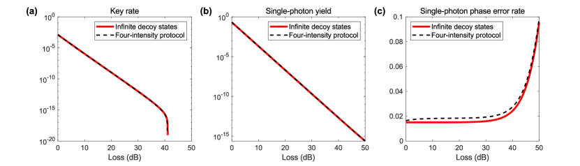
Figure S11: Comparison of calculation results of infinite decoy-state method and four-intensity method. (a) key rate; (b) single-photon yield; (c) single-photon phase error rate. The parameters used in the calculation are: detection efficiency $\eta_{d}=0.93$, dark count rate $p_{d}=10^{-7}$, misalignment error $e_{d}=1.5\%$.

S3.3.2 Comparison with three-intensity decoy-state method in non-asymptotic case

We simulate the conference key rate for the three-intensity and four-intensity protocol under different conditions. The parameters used in the simulation are shown in the table below:

$p_{d}$	$\eta_{d}$	$e_{d}$	$f$	$\varepsilon$	$V$
$10^{-6}$	$0.8$	$0.025$	$1.16$	$10^{-10}$	$0.25$

Table S3: Parameters in simulation

The secure key rate formula of three-intensity protocol we use in simulation is:

$$R_{\text{three-intensity}}=(p_{Z|\mu}p_{\mu})^{3}\left\{\mu^{3}e^{-3\mu}{Y}_{111}^{Z,L}\left[1-H({e}_{111}^{PZ,U})\right]-Q_{\mu\mu\mu}^{Z}fH(E^{Z}_{\mu\mu\mu})\right\},$$ (S3.104)

where $\mu$ is the average photon number of the signal state pulses, $p_{\mu}$ is the probability of selecting the signal source, $p_{Z|\mu}$ is the probability of encoding pulses on Z-basis under the condition of selecting the signal source, ${Y}_{111}^{Z,L}$ is the lower bound of the yield of Z-basis single-photon component, ${e}_{111}^{PZ,U}$ is the upper bound of the phase error rate of Z-basis single-photon component; $Q_{\mu\mu\mu}^{Z}$ and $E^{Z}_{\mu\mu\mu}$ is the overall gain and the quantum bit error rate of the Z-basis pulses from the signal source respectively. In the numerical simulation of the three-intensity protocol, the key rate is the function of six parameters: $\mu$, $\nu$, $p_{\mu}$, $p_{\nu}$, $p_{Z|\mu}$ and $p_{Z|\nu}$. We implement the full parameter optimization.

We first compare the optimal key rates of the two protocols under different total channel losses for $N=10^{13}$ and $N=10^{14}$, respectively. The results show that the key rate and the communication distance of the four-intensity protocol is tremendously improved over the three-intensity protocol in both cases. In particular, there is a one- to two-order-of-magnitude improvement in the conference key rate when the number of pulses is small and the total channel loss is large. On the other hand, we perform key rate optimization by varying the number of pulses with a total channel loss of 18 dB. The results show that the four-intensity protocol can generate the secure key by sending only $3.5\times 10^{12}$ pulses, however, the three-intensity protocol requires a minimum of about $4\times 10^{13}$. This implies that the four-intensity protocol has a lower threshold for the number of pulses required for generating key and is therefore experimentally easier to implement.

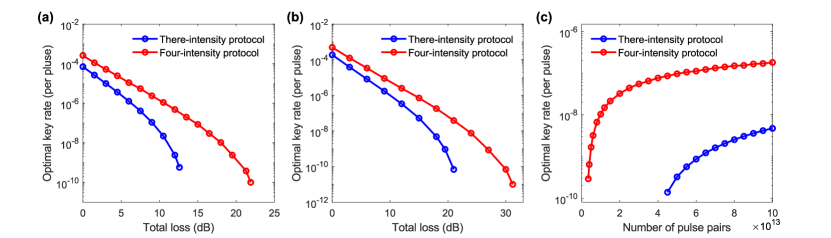
Figure S12: Optimal conference key rate of three-intensity protocol and four-intensity protocol. (a) $N=10^{13}$. (b) $N=10^{14}$. (c) Optimal key rate at a total loss of 18 dB with different pulse numbers sent by users.

	$N=10^{13}$		$N=10^{14}$
Total loss (dB)	$6.0$	$12.0$	$9.0$	$18.0$
$R_{\text{3-int}}$	$1.267\times 10^{-6}$	$2.385\times 10^{-9}$	$1.720\times 10^{-6}$	$4.764\times 10^{-9}$
$R_{\text{4-int}}$	$1.101\times 10^{-5}$	$4.820\times 10^{-7}$	$8.949\times 10^{-6}$	$1.804\times 10^{-7}$
$R_{\text{4-int}}/R_{\text{3-int}}$	$8.69$	$202.10$	$5.20$	$37.87$

Table S4: Comparison of conference key rate of two protocols for different sent pulse number and channel loss.

S4 S4: Experimental results

Overall attenuation (dB)	$\eta$	14.1	17.8	21.5
Number of        pulse pairs	$N_{zzz}$	$7.2000\times 10^{11}$
	$N_{xxx}$	$2.6528\times 10^{12}$
	$N_{yyy}$	$1.6000\times 10^{10}$
	$N_{ooo}$	$6.0000\times 10^{9}$
	$N_{oxx}+N_{xox}+N_{xxo}$	$1.1040\times 10^{12}$
	$N_{xoo}+N_{oxo}+N_{oox}$	$1.4400\times 10^{11}$
	$N_{oyy}+N_{yoy}+N_{yyo}$	$2.4000\times 10^{10}$
	$N_{yoo}+N_{oyo}+N_{ooy}$	$2.4000\times 10^{10}$
Total gains	$M_{zzz}$	$6851252$	$3061962$	$1248883$
	$M_{xxx}$	$2207217$	$951388$	$408827$
	$M_{yyy}$	$1941154$	$857992$	$373106$
	$M_{oyy}$	$233950$	$105880$	$44065$
	$M_{yoy}$	$280433$	$114446$	$49702$
	$M_{yyo}$	$261515$	$118246$	$49535$
	$M_{yoo}$	$176$	$60$	$29$
	$M_{oyo}$	$5$	$3$	$0$
	$M_{ooy}$	$380$	$115$	$49$
	$M_{ooo}$	$0$	$0$	$0$
	$M_{oxx}+M_{xox}+M_{xxo}$	$237638$	$101573$	$42814$
	$M_{xoo}+M_{oxo}+M_{oox}$	$35$	$14$	$6$
Error gains	$E_{zzz}^{AB}$	$131768$	$68298$	$22716$
	$E_{zzz}^{AC}$	$132496$	$71445$	$23973$
	$E_{zzz}^{BC}$	$150078$	$73779$	$26937$
	$E_{xxx}$	$882539$	$379058$	$162357$
	$E_{yyy}$	$831142$	$368415$	$158805$
Results	$e_{Z}^{AB}$ (%)	$1.92$	$2.23$	$1.82$
	$e_{Z}^{AC}$ (%)	$1.93$	$2.33$	$1.92$
	$e_{Z}^{BC}$ (%)	$2.19$	$2.41$	$2.16$
	$e_{111}^{PZ}$ (%)	$15.04$	$17.63$	$22.16$
	$Y_{111}^{Z}$	$8.70\times 10^{-3}$	$3.86\times 10^{-3}$	$1.78\times 10^{-3}$
	key rate (per pulse)	$3.02\times 10^{-8}$	$4.69\times 10^{-9}$	$3.86\times 10^{-10}$

Table S5: Detailed results of the MDI-QCC experiment. The subscripts indicate the photon sources of three users. We remark that the SNSPDs have the detection efficiency of about 80% and the dark count rate of about $10^{-6}$. To reduce the error rate, we set the coincidence time window to 156.25 ps in the data processing. The efficiency of the coincidence time window is about 87%, 90%, 91% for the data of overall attenuation of 14.1 dB, 17.8 dB and 21.5 dB respectively.

References

• Bennett and Brassard [1984] C. H. Bennett and G. Brassard, Quantum cryptography: Public key distribution and coin tossing, in Proceedings of IEEE International Conference on Computers, Systems, and Signal Processing (IEEE, New York, 1984) p. 175–179.
• Ekert [1991] A. K. Ekert, Quantum cryptography based on bell’s theorem, Phys. Rev. Lett. 67, 661 (1991).
• Gisin et al. [2002] N. Gisin, G. Ribordy, W. Tittel, and H. Zbinden, Quantum cryptography, Rev. Mod. Phys. 74, 145 (2002).
• Scarani et al. [2009] V. Scarani, H. Bechmann-Pasquinucci, N. J. Cerf, M. Dušek, N. Lütkenhaus, and M. Peev, The security of practical quantum key distribution, Rev. Mod. Phys. 81, 1301 (2009).
• Xu et al. [2020] F. Xu, X. Ma, Q. Zhang, H.-K. Lo, and J.-W. Pan, Secure quantum key distribution with realistic devices, Rev. Mod. Phys. 92, 025002 (2020).
• Pirandola et al. [2020] S. Pirandola, U. L. Andersen, L. Banchi, M. Berta, D. Bunandar, R. Colbeck, D. Englund, T. Gehring, C. Lupo, C. Ottaviani, J. L. Pereira, M. Razavi, J. S. Shaari, M. Tomamichel, V. C. Usenko, G. Vallone, P. Villoresi, and P. Wallden, Advances in quantum cryptography, Adv. Opt. Photon. 12, 1012 (2020).
• Hwang [2003] W.-Y. Hwang, Quantum key distribution with high loss: Toward global secure communication, Phys. Rev. Lett. 91, 057901 (2003).
• Wang [2005] X.-B. Wang, Beating the photon-number-splitting attack in practical quantum cryptography, Phys. Rev. Lett. 94, 230503 (2005).
• Lo et al. [2005] H.-K. Lo, X. Ma, and K. Chen, Decoy state quantum key distribution, Phys. Rev. Lett. 94, 230504 (2005).
• Acín et al. [2007] A. Acín, N. Brunner, N. Gisin, S. Massar, S. Pironio, and V. Scarani, Device-independent security of quantum cryptography against collective attacks, Phys. Rev. Lett. 98, 230501 (2007).
• Braunstein and Pirandola [2012] S. L. Braunstein and S. Pirandola, Side-channel-free quantum key distribution, Phys. Rev. Lett. 108, 130502 (2012).
• Lo et al. [2012] H.-K. Lo, M. Curty, and B. Qi, Measurement-device-independent quantum key distribution, Phys. Rev. Lett. 108, 130503 (2012).
• Lucamarini et al. [2018] M. Lucamarini, Z. L. Yuan, J. F. Dynes, and A. J. Shields, Overcoming the rate–distance limit of quantum key distribution without quantum repeaters, Nature 557, 400 (2018).
• Zeng et al. [2022] P. Zeng, H. Zhou, W. Wu, and X. Ma, Mode-pairing quantum key distribution, Nature Communications 13, 3903 (2022).
• Xie et al. [2022] Y.-M. Xie, Y.-S. Lu, C.-X. Weng, X.-Y. Cao, Z.-Y. Jia, Y. Bao, Y. Wang, Y. Fu, H.-L. Yin, and Z.-B. Chen, Breaking the rate-loss bound of quantum key distribution with asynchronous two-photon interference, PRX Quantum 3, 020315 (2022).
• Yin et al. [2020] J. Yin, Y.-H. Li, S.-K. Liao, M. Yang, Y. Cao, L. Zhang, J.-G. Ren, W.-Q. Cai, W.-Y. Liu, S.-L. Li, R. Shu, Y.-M. Huang, L. Deng, L. Li, Q. Zhang, N.-L. Liu, Y.-A. Chen, C.-Y. Lu, X.-B. Wang, F. Xu, J.-Y. Wang, C.-Z. Peng, A. K. Ekert, and J.-W. Pan, Entanglement-based secure quantum cryptography over 1,120 kilometres, Nature 582, 501 (2020).
• Chen et al. [2021] Y.-A. Chen, Q. Zhang, T.-Y. Chen, W.-Q. Cai, S.-K. Liao, J. Zhang, K. Chen, J. Yin, J.-G. Ren, Z. Chen, S.-L. Han, Q. Yu, K. Liang, F. Zhou, X. Yuan, M.-S. Zhao, T.-Y. Wang, X. Jiang, L. Zhang, W.-Y. Liu, Y. Li, Q. Shen, Y. Cao, C.-Y. Lu, R. Shu, J.-Y. Wang, L. Li, N.-L. Liu, F. Xu, X.-B. Wang, C.-Z. Peng, and J.-W. Pan, An integrated space-to-ground quantum communication network over 4,600 kilometres, Nature 589, 214 (2021).
• Liu et al. [2023] Y. Liu, W.-J. Zhang, C. Jiang, J.-P. Chen, C. Zhang, W.-X. Pan, D. Ma, H. Dong, J.-M. Xiong, C.-J. Zhang, H. Li, R.-C. Wang, J. Wu, T.-Y. Chen, L. You, X.-B. Wang, Q. Zhang, and J.-W. Pan, Experimental twin-field quantum key distribution over 1000 km fiber distance, Phys. Rev. Lett. 130, 210801 (2023).
• Li et al. [2023] W. Li, L. Zhang, H. Tan, Y. Lu, S.-K. Liao, J. Huang, H. Li, Z. Wang, H.-K. Mao, B. Yan, Q. Li, Y. Liu, Q. Zhang, C.-Z. Peng, L. You, F. Xu, and J.-W. Pan, High-rate quantum key distribution exceeding 110 mb s–1, Nature Photonics 17, 416 (2023).
• Kimble [2008] H. J. Kimble, The quantum internet, Nature 453, 1023 (2008).
• Wehner et al. [2018] S. Wehner, D. Elkouss, and R. Hanson, Quantum internet: A vision for the road ahead, Science 362, eaam9288 (2018).
• Wengerowsky et al. [2018] S. Wengerowsky, S. K. Joshi, F. Steinlechner, H. Hübel, and R. Ursin, An entanglement-based wavelength-multiplexed quantum communication network, Nature 564, 225 (2018).
• Joshi et al. [2020] S. K. Joshi, D. Aktas, S. Wengerowsky, M. Lončarić, S. P. Neumann, B. Liu, T. Scheidl, G. C. Lorenzo, Željko Samec, L. Kling, A. Qiu, M. Razavi, M. Stipčević, J. G. Rarity, and R. Ursin, A trusted node–free eight-user metropolitan quantum communication network, Science Advances 6, eaba0959 (2020).
• Wen et al. [2022] W. Wen, Z. Chen, L. Lu, W. Yan, W. Xue, P. Zhang, Y. Lu, S. Zhu, and X.-S. Ma, Realizing an entanglement-based multiuser quantum network with integrated photonics, Phys. Rev. Appl. 18, 024059 (2022).
• Bose et al. [1998] S. Bose, V. Vedral, and P. L. Knight, Multiparticle generalization of entanglement swapping, Phys. Rev. A 57, 822 (1998).
• Chen and Lo [2004] K. Chen and H.-K. Lo, Multipartite quantum cryptographic protocols with noisy ghz states, Quantum Information and Computation 7 (2004).
• Murta et al. [2020] G. Murta, F. Grasselli, H. Kampermann, and D. Bruß, Quantum conference key agreement: A review, Advanced Quantum Technologies 3, 2000025 (2020).
• Hillery et al. [1999] M. Hillery, V. Bužek, and A. Berthiaume, Quantum secret sharing, Phys. Rev. A 59, 1829 (1999).
• Cleve et al. [1999] R. Cleve, D. Gottesman, and H.-K. Lo, How to share a quantum secret, Phys. Rev. Lett. 83, 648 (1999).
• Tittel et al. [2001] W. Tittel, H. Zbinden, and N. Gisin, Experimental demonstration of quantum secret sharing, Phys. Rev. A 63, 042301 (2001).
• Chen et al. [2005] Y.-A. Chen, A.-N. Zhang, Z. Zhao, X.-Q. Zhou, C.-Y. Lu, C.-Z. Peng, T. Yang, and J.-W. Pan, Experimental quantum secret sharing and third-man quantum cryptography, Phys. Rev. Lett. 95, 200502 (2005).
• Schmid et al. [2005] C. Schmid, P. Trojek, M. Bourennane, C. Kurtsiefer, M. Żukowski, and H. Weinfurter, Experimental single qubit quantum secret sharing, Phys. Rev. Lett. 95, 230505 (2005).
• Gaertner et al. [2007] S. Gaertner, C. Kurtsiefer, M. Bourennane, and H. Weinfurter, Experimental demonstration of four-party quantum secret sharing, Phys. Rev. Lett. 98, 020503 (2007).
• Bell et al. [2014] B. A. Bell, D. Markham, D. A. Herrera-Martí, A. Marin, W. J. Wadsworth, J. G. Rarity, and M. S. Tame, Experimental demonstration of graph-state quantum secret sharing, Nature Communications 5, 5480 (2014).
• Lee et al. [2020] S. M. Lee, S.-W. Lee, H. Jeong, and H. S. Park, Quantum teleportation of shared quantum secret, Phys. Rev. Lett. 124, 060501 (2020).
• Augusiak and Horodecki [2009] R. Augusiak and P. Horodecki, Multipartite secret key distillation and bound entanglement, Phys. Rev. A 80, 042307 (2009).
• Das et al. [2021] S. Das, S. Bäuml, M. Winczewski, and K. Horodecki, Universal limitations on quantum key distribution over a network, Phys. Rev. X 11, 041016 (2021).
• Carrara et al. [2021] G. Carrara, H. Kampermann, D. Bruß, and G. Murta, Genuine multipartite entanglement is not a precondition for secure conference key agreement, Phys. Rev. Res. 3, 013264 (2021).
• Greenberger et al. [1989] D. M. Greenberger, M. A. Horne, and A. Zeilinger, Going beyond bell’s theorem, in Bell’s Theorem, Quantum Theory and Conceptions of the Universe, edited by M. Kafatos (Springer Netherlands, Dordrecht, 1989) pp. 69–72.
• Dür et al. [2000] W. Dür, G. Vidal, and J. I. Cirac, Three qubits can be entangled in two inequivalent ways, Phys. Rev. A 62, 062314 (2000).
• Epping et al. [2017] M. Epping, H. Kampermann, C. macchiavello, and D. Bruß, Multi-partite entanglement can speed up quantum key distribution in networks, New Journal of Physics 19, 093012 (2017).
• Grasselli et al. [2018] F. Grasselli, H. Kampermann, and D. Bruß, Finite-key effects in multipartite quantum key distribution protocols, New Journal of Physics 20, 113014 (2018).
• Fu et al. [2015] Y. Fu, H.-L. Yin, T.-Y. Chen, and Z.-B. Chen, Long-distance measurement-device-independent multiparty quantum communication, Phys. Rev. Lett. 114, 090501 (2015).
• Grasselli et al. [2019] F. Grasselli, H. Kampermann, and D. Bruß, Conference key agreement with single-photon interference, New Journal of Physics 21, 123002 (2019).
• Zhao et al. [2020] S. Zhao, P. Zeng, W.-F. Cao, X.-Y. Xu, Y.-Z. Zhen, X. Ma, L. Li, N.-L. Liu, and K. Chen, Phase-matching quantum cryptographic conferencing, Phys. Rev. Appl. 14, 024010 (2020).
• Cao et al. [2021a] X.-Y. Cao, Y.-S. Lu, Z. Li, J. Gu, H.-L. Yin, and Z.-B. Chen, High key rate quantum conference key agreement with unconditional security, IEEE Access 9, 128870 (2021a).
• Cao et al. [2021b] X.-Y. Cao, J. Gu, Y.-S. Lu, H.-L. Yin, and Z.-B. Chen, Coherent one-way quantum conference key agreement based on twin field, New Journal of Physics 23, 043002 (2021b).
• Bai et al. [2022] J.-L. Bai, Y.-M. Xie, Z. Li, H.-L. Yin, and Z.-B. Chen, Post-matching quantum conference key agreement, Optics Express 30, 28865 (2022).
• Carrara et al. [2023] G. Carrara, G. Murta, and F. Grasselli, Overcoming fundamental bounds on quantum conference key agreement, Phys. Rev. Appl. 19, 064017 (2023).
• Lu et al. [2024] Y.-S. Lu, Y.-M. Xie, Y. Fu, H.-L. Yin, and Z.-B. Chen, Repeater-like asynchronous measurement-device-independent quantum conference key agreement (2024), arXiv:2406.15853 [quant-ph] .
• Xie et al. [2024] Y.-M. Xie, Y.-S. Lu, Y. Fu, H.-L. Yin, and Z.-B. Chen, Multi-field quantum conferencing overcomes the network capacity limit (2024), arXiv:2407.00897 [quant-ph] .
• Proietti et al. [2021] M. Proietti, J. Ho, F. Grasselli, P. Barrow, M. Malik, and A. Fedrizzi, Experimental quantum conference key agreement, Science Advances 7, eabe0395 (2021).
• Pickston et al. [2023] A. Pickston, J. Ho, A. Ulibarrena, F. Grasselli, M. Proietti, C. L. Morrison, P. Barrow, F. Graffitti, and A. Fedrizzi, Conference key agreement in a quantum network, npj Quantum Information 9, 82 (2023).
• Zhou et al. [2016] Y.-H. Zhou, Z.-W. Yu, and X.-B. Wang, Making the decoy-state measurement-device-independent quantum key distribution practically useful, Phys. Rev. A 93, 042324 (2016).
• [55] See the section 3 of the Supplemetal Materials for detailed analysis of the four-intensity MDI-QCC protocol.
• Pan and Zeilinger [1998] J.-W. Pan and A. Zeilinger, Greenberger-horne-zeilinger-state analyzer, Phys. Rev. A 57, 2208 (1998).
• Pan et al. [2012] J.-W. Pan, Z.-B. Chen, C.-Y. Lu, H. Weinfurter, A. Zeilinger, and M. Żukowski, Multiphoton entanglement and interferometry, Rev. Mod. Phys. 84, 777 (2012).
• Li et al. [2019] Y. Li, Y.-H. Li, H.-B. Xie, Z.-P. Li, X. Jiang, W.-Q. Cai, J.-G. Ren, J. Yin, S.-K. Liao, and C.-Z. Peng, High-speed robust polarization modulation for quantum key distribution, Optics Letters 44, 5262 (2019).
• Luo et al. [2022] W. Luo, Y. Li, Y. Li, X. Tao, L. Han, W. Cai, J. Yin, J. Ren, S. Liao, and C. Peng, Intrinsically stable 2-ghz polarization modulation for satellite-based quantum key distribution, IEEE Photonics Journal 14, 1 (2022).
• Lu et al. [2009] C.-Y. Lu, T. Yang, and J.-W. Pan, Experimental multiparticle entanglement swapping for quantum networking, Phys. Rev. Lett. 103, 020501 (2009).
• Jing et al. [2019] B. Jing, X.-J. Wang, Y. Yu, P.-F. Sun, Y. Jiang, S.-J. Yang, W.-H. Jiang, X.-Y. Luo, J. Zhang, X. Jiang, X.-H. Bao, and J.-W. Pan, Entanglement of three quantum memories via interference of three single photons, Nature Photonics 13, 210 (2019).
• Pramanik et al. [2020] T. Pramanik, D.-H. Lee, Y.-W. Cho, H.-T. Lim, S.-W. Han, H. Jung, S. Moon, K. J. Lee, and Y.-S. Kim, Equitable multiparty quantum communication without a trusted third party, Phys. Rev. Appl. 14, 064074 (2020).
• Hong et al. [1987] C. K. Hong, Z. Y. Ou, and L. Mandel, Measurement of subpicosecond time intervals between two photons by interference, Phys. Rev. Lett. 59, 2044 (1987).
• Herman [1952] C. Herman, A measure of asymptotic efficiency for tests of a hypothesis based on the sum of observations, The Annals of Mathematical Statistics 23, 493 (1952).
• Li and Zhao [2022] W. Li and S. Zhao, Security research on practical measurement-device-independent quantum key distribution, Phys. Rev. A 106, 042445 (2022).
• Zhang et al. [2017] Z. Zhang, Q. Zhao, M. Razavi, and X. Ma, Improved key-rate bounds for practical decoy-state quantum-key-distribution systems, Phys. Rev. A 95, 012333 (2017).
• Jiang et al. [2021] C. Jiang, Z.-W. Yu, X.-L. Hu, and X.-B. Wang, Higher key rate of measurement-device-independent quantum key distribution through joint data processing, Phys. Rev. A 103, 012402 (2021).