Uncertain standard quadratic optimization
under distributional assumptions:
a chance-constrained epigraphic approach

Abstract

The standard quadratic optimization problem (StQP) consists of minimizing a quadratic form over the standard simplex. Without convexity or concavity of the quadratic form, the StQP is NP-hard. This problem has many relevant real-life applications ranging from portfolio optimization to pairwise clustering and replicator dynamics.

Sometimes, the data matrix is uncertain. We investigate models where the distribution of the data matrix is known but where both the StQP after realization of the data matrix and the here-and-now problem are indefinite. We test the performance of a chance-constrained epigraphic StQP to the uncertain StQP.

Keywords: Stochastic optimization, Quadratic optimization, Chance constraints, Gaussian Orthogonal Ensemble
MSC(2020) Classification: 90C20, 90C15, 90C26

1 Introduction

The standard quadratic optimization problem consists of minimizing a quadratic form over the standard simplex

$$\ell({\mathsf{Q}}):=\min_{{\mathbf{x}}\in\Delta}\,{\mathbf{x}}^{\top}{\mathsf{Q}}{\mathbf{x}}$$ (1)

where ${\mathsf{Q}}\in\mathbb{R}^{n\times n}$ is a symmetric matrix, and $\Delta:=\{{\mathbf{x}}\in\mathbb{R}^{n}:{\mathbf{e}}^{\top}{\mathbf{x}}=1,{\mathbf{x}}\geq\bm{0}\}$ is the standard simplex in $\mathbb{R}^{n}$. Here ${\mathbf{e}}\in\mathbb{R}^{n}$ is the vector of all ones and ^⊤ denotes transposition; ${\mathsf{I}}={\rm Diag}({\mathbf{e}})$ denotes the $n\times n$ identity matrix. The objective function is already in general form since any general quadratic objective function ${\mathbf{x}}^{\top}{\mathsf{A}}{\mathbf{x}}+2{\mathbf{c}}^{\top}{\mathbf{x}}$ can be written in homogeneous form by defining the symmetric matrix ${\mathsf{Q}}:={\mathsf{A}}+{\mathbf{c}}{\mathbf{e}}^{\top}+{\mathbf{e}}{\mathbf{c}}^{\top}$.

Even though the StQP is simple - minimization of a quadratic function under linear constraints - it is NP-hard without assumptions on the definiteness of the matrix ${\mathsf{Q}}$; observe that convex, but also concave instances are polynomially solvable, the latter even in closed form: $\ell({\mathsf{Q}})=\min_{i}{\mathsf{Q}}_{ii}$. Note that $\ell({\mathsf{Q}})\geq 0$ is possible even if ${\mathsf{Q}}$ is not positive semi-definite. In fact, the condition $\ell({\mathsf{Q}})\geq 0$ characterizes copositivity [14] of ${\mathsf{Q}}$, and follows if no entry of ${\mathsf{Q}}$ is negative (as, e.g. in the instances ${\mathsf{Q}}_{i}^{\rm(nom)}$ generated in Section 5 below).

Irrespective of the sign of $\ell({\mathsf{Q}})$, its calculation can be hard for indefinite instances: indeed, Motzkin and Straus [12] showed that the maximum clique problem, a well-known NP-hard problem, can be formulated as an StQP. Hence, the StQP is often regarded as the simplest of hard problems [3] since it contains the simplest non-convex objective function which is a quadratic form, and the simplest polytope as feasible set. Still, the StQP is a very flexible optimization class that allows for modelling of diverse problems such as portfolio optimization problems [11], pairwise clustering [13] and replicator dynamics [2]. Despite of its continuous (in fact, quadratic) optimization nature, it also serves to model discrete problems like the maximum-clique problem as well, as witnessed by above references.

The only data required to fully characterize an StQP is the data matrix ${\mathsf{Q}}$. However, in many applications the matrix ${\mathsf{Q}}$ is uncertain. StQPs with uncertain data have been explored in the literature. One of the most natural ways to deal with uncertain objective functions is the worst-case approach, where there is no information on the distribution of the data matrix ${\mathsf{Q}}$ except for its support. Bomze et al. [4] introduced the concept of a robust standard quadratic optimization problem, which they formulated as a minimax problem

$$\min_{{\mathbf{x}}\in\Delta}\max_{{\mathsf{U}}\in\mathcal{U}}\,{\mathbf{x}}^{\top}({\mathsf{Q}}^{\rm(nom)}+{\mathsf{U}}){\mathbf{x}}.$$ (2)

with uncertainty set $\mathcal{U}$. The uncertain matrix ${\mathsf{Q}}$ consisted of a nominal part ${\mathsf{Q}}^{\rm(nom)}$ and an uncertain additive perturbation ${\mathsf{U}}$. In their paper, the authors investigated various uncertainty sets and proved that the copositive relaxation gap is equal to the minimax gap. Moreover, they observed that the robust StQP (2) reduces to a deterministic StQP for many frequently used types of uncertainty sets $\mathcal{U}$.

Passing from a robust to stochastic setting with known expectation, a natural alternative to get rid of the uncertainty is the here-and-now problem (random quantities are designated by a tilde sign)

$$\min_{{\mathbf{x}}\in\Delta}\,\mathbb{E}[{\mathbf{x}}^{\top}\widetilde{\mathsf{Q}}{\mathbf{x}}]=\min_{{\mathbf{x}}\in\Delta}\,{\mathbf{x}}^{\top}\mathbb{E}[\widetilde{\mathsf{Q}}]{\mathbf{x}}$$ (3)

where the uncertain matrix $\widetilde{\mathsf{Q}}$ is replaced by its expectation $\mathbb{E}[\widetilde{\mathsf{Q}}]$. In this paper, we propose an alternative to the here-and-now problem. Bomze et al. [5] investigated a two-stage setting where the principal submatrix was deterministic and the rest of the entries followed a known probability distribution. In this paper, we will however assume that the full data matrix $\widetilde{\mathsf{Q}}$ is stochastic with known distribution $\mathbb{P}$, in which case models with two stages are less meaningful. The purpose of this note is to introduce, apparently for the first time, chance constraints for this problem class by introduction of an epigraphic variable, and moreover, to present a deterministic equivalent StQP formulation under reasonable distributional assumptions. Moreover, we establish a close connection of our new model to robustness with Frobenius ball uncertainty sets.

2 Chance-constrained epigraphic StQP

It is well known that any optimization problem

$$\min_{{\mathbf{x}}\in\mathcal{X}}\,f({\mathbf{x}})$$

can be rewritten equivalently in epigraphic form by introducing an extra variable $t$

$$\underset{{\mathbf{x}},t}{\min} \quad t$$

s.t. $$\quad f({\mathbf{x}})\leq t$$ (4a)

$$\quad{\mathbf{x}}\in\mathcal{X},\,t\in\mathbb{R}.$$ (4b)

Now suppose that $f:\mathbb{R}^{n}\times\mathbb{R}^{p}\to\mathbb{R}$ is a random objective function that depends on the decision variable ${\mathbf{x}}\in\mathcal{X}\subseteq\mathbb{R}^{n}$ and on the random vector $\bm{\tilde{\xi}}\in\Omega\subseteq\mathbb{R}^{p}$. For every fixed ${\mathbf{x}}\in\mathcal{X}$, $f({\mathbf{x}},\bm{\tilde{\xi}})$ is a random variable with a distribution $\mathbb{P}$. Then we can regard constraint (4a) as a soft constraint and request feasibility with probability of at least $\alpha$ to obtain (5). Constraint (4b) remains a hard constraint and must be satisfied for all feasible points. This has a familiar interpretation familiar in risk management as the so-called value-at-risk (VaR) of $f({\mathbf{x}},\bm{\tilde{\xi}})$ at ${\mathbf{x}}$ with confidence level $\alpha\in(0,1)$, defined as [9]

$$\text{VaR}_{\alpha}({\mathbf{x}}):=\min\,\{t:\mathbb{P}[f({\mathbf{x}},\bm{\tilde{\xi}})\leq t]\geq\alpha\}.$$

The problem of minimizing VaR [8] is

$$\begin{array}[]{lcl}\underset{{\mathbf{x}}\in\mathcal{X}}{\min}\,\text{VaR}_{\alpha}({\mathbf{x}})=&\underset{{\mathbf{x}},t}{\min}&t\\ &\text{s.t.}&\mathbb{P}[f({\mathbf{x}},\bm{\tilde{\xi}})\leq t]\geq\alpha\\ &&{\mathbf{x}}\in\mathcal{X},\,t\in\mathbb{R}\,.\end{array}$$ (5)

El Ghaoui et al. [6] investigated problem (5) in the context of worst-case VaR for portfolio optimization with a return function

$$f({\mathbf{x}},\bm{\tilde{\xi}}):={\mathbf{x}}^{\top}\bm{\tilde{\xi}}$$

where $\bm{\tilde{\xi}}$ was a vector of returns. Inspired by the VaR and passing from linear to quadratic expressions in the decision variable ${\mathbf{x}}$, we want to find the smallest number $t\in\mathbb{R}$ such that ${\mathbf{x}}^{\top}\widetilde{\mathsf{Q}}{\mathbf{x}}\leq t$ with probability at least $\alpha$, where $\alpha\in(0,1)$ is a confidence level provided by the decision-maker. This means solving the following stochastic optimization problem which we call chance-constrained epigraphic StQP

$$\begin{array}[]{lcl}\ell^{\rm(cce)}_{\mathbb{P},\alpha}:=&\underset{{\mathbf{x}},t}{\min}&t\\ &\text{s.t.}&\mathbb{P}({\mathbf{x}}^{\top}\widetilde{\mathsf{Q}}{\mathbf{x}}\leq t)\geq\alpha\\ &&{\mathbf{x}}\in\Delta\,,\,t\in\mathbb{R}\,.\end{array}$$ (CCE-StQP)

3 Distributional uncertainty models

Two common and simple ways of generating an indefinite random symmetric matrix $\widetilde{\mathsf{Q}}$ are:

1. Generate a random $n\times n$ matrix $\widetilde{\mathsf{R}}$ and put $\widetilde{\mathsf{Q}}:={\mathsf{Q}}^{\rm(nom)}+\frac{\beta}{\sqrt{2}}(\widetilde{\mathsf{R}}+\widetilde{\mathsf{R}}^{\top})$, for some nominal matrix ${\mathsf{Q}}^{\rm(nom)}$ and parameter $\beta$.

2. Generate a random $r\times n$ matrix $\widetilde{\mathsf{F}}$ and put $\widetilde{\mathsf{Q}}:=\widetilde{\mathsf{F}}^{\top}\widetilde{\mathsf{F}}$. This generates a convex instance, but it can be avoided by subtracting $\eta\,{\mathsf{I}}$ for large enough $\eta>0$, but not too large to avoid concave instances.

In case that $\widetilde{\mathsf{R}}$ or $\widetilde{\mathsf{F}}$ are normal with i.i.d. entries we obtain the shifted/scaled GOE in the first case and the shifted Wishart distribution in the second case [7, 10, 16]. More generally, suppose that $\mathbb{P}$ enjoys the following property:

Property 1.

For all ${\mathbf{x}}\in\Delta$, the distribution of ${\mathbf{x}}^{\top}\widetilde{\mathsf{Q}}{\mathbf{x}}$ is of location/scale type where for some continuous cdf $F$ which is strictly increasing on $\{t\in\mathbb{R}:F(t)>0\}$

$$\mathbb{P}({\mathbf{x}}^{\top}\widetilde{\mathsf{Q}}{\mathbf{x}}\leq t)=F\left(\frac{t-\mu({\mathbf{x}})}{\sigma({\mathbf{x}})}\right)$$

with two parameters depending on ${\mathbf{x}}$ in the following way:

$$\mu({\mathbf{x}})={\mathbf{x}}^{\top}{\mathsf{M}}{\mathbf{x}},\quad\sigma({\mathbf{x}})={\mathbf{x}}^{\top}{\mathsf{S}}{\mathbf{x}}>0,$$

where ${\mathsf{M}}$ and ${\mathsf{S}}$ are symmetric $n\times n$ matrices.

Remark 2.

Property 1 is satisfied for both GOE (with ${\mathsf{M}}={\mathsf{Q}}^{\rm(nom)},\,{\mathsf{S}}=\beta\,{\mathsf{I}}$ and $F=\Phi$, see Corollary 6 below) and shifted Wishart (with ${\mathsf{M}}=-\eta\,{\mathsf{I}},{\mathsf{S}}=2{\bm{\Sigma}}$). Indeed, for $\widetilde{\mathsf{Q}}:=\widetilde{\mathsf{W}}-\eta\,{\mathsf{I}}$ with Wishart matrix $\widetilde{\mathsf{W}}\sim\mathcal{W}_{n}({\bm{\Sigma}},p)$ we have that ${\mathbf{x}}^{\top}\widetilde{\mathsf{W}}{\mathbf{x}}$ is a gamma distributed random variable with shape $k=p/2$ and scale $\theta=2{\mathbf{x}}^{\top}{\bm{\Sigma}}{\mathbf{x}}$, where $p$ determines the shape of $F$.

Then the CCE-StQP can be reformulated as a deterministic StQP.

Theorem 3.

Under Property 1, we get for $\overline{\mathsf{Q}}:={\mathsf{M}}+F^{-1}(\alpha){\mathsf{S}}$

$$\ell(\overline{\mathsf{Q}})=\ell^{\rm(cce)}_{\mathbb{P},\alpha}\,.$$

Proof.

A feasible pair $({\mathbf{x}},t)\in\Delta\times\mathbb{R}$ satisfies

$$\mathbb{P}({\mathbf{x}}^{\top}\widetilde{\mathsf{Q}}{\mathbf{x}}\leq t)\geq\alpha\quad\text{ if and only if }\quad{\mathbf{x}}^{\top}\overline{\mathsf{Q}}{\mathbf{x}}\leq t.$$

Hence $\ell(\overline{\mathsf{Q}})$ is an epigraphic formulation of $\ell^{\rm(cce)}_{\mathbb{P},\alpha}$. ∎

Hence we have established a deterministic StQP equivalent of the CCE-StQP under reasonable distributional assumptions. This is in line with several robust counterparts [4].

Now for a special case, we find an even closer connection to some special robust StQP models, namely with Frobenius balls as uncertainty set; see the following section.

4 Gaussian Orthogonal Ensemble perturbation

An appropriate model for real symmetric random matrices are Wigner matrices [17] with i.i.d. diagonal entries and also i.i.d. entries above the diagonal, both with finite second moments. Wigner’s semicircle law states that for off-diagonals centered at zero and and denoting by $\tau$ the second moment of the off-diagonals, the empirical spectral measure (count of eigenvalues in a certain interval), scaled by $\frac{1}{\sqrt{n}}$, converges weakly to the Wigner semicircle distribution with density

$$\mu_{sc}(x):=\frac{1}{2\pi\tau^{2}}\sqrt{(4\tau^{2}-x^{2})_{+}}\,.$$

The Gaussian Orthogonal Ensemble (GOE) consists of Wigner matrices $\widetilde{\mathsf{G}}=(\widetilde{g}_{ij})$ such that $\widetilde{g}_{ii}$ are i.i.d. with $\widetilde{g}_{ii}\sim\mathcal{N}(0,2)$, for $i=1,\dots,n$ and $\widetilde{g}_{ij}$ are i.i.d. standard normal random variables, $\widetilde{g}_{ij}\sim\mathcal{N}(0,1)$, for $1\leq i<j\leq n$. Perturbation of a nominal matrix by a GOE matrix has been extensively explored in the literature, see [1], [15].

In our distributional uncertainty model, suppose that the random matrix $\widetilde{\mathsf{Q}}$ is of the following form

$$\widetilde{\mathsf{Q}}={\mathsf{Q}}^{\rm(nom)}+\beta\,\widetilde{\mathsf{G}}$$ (6)

where the real symmetric nominal matrix ${\mathsf{Q}}^{\rm(nom)}$ is perturbed by a GOE matrix $\widetilde{\mathsf{G}}$ multiplied by a factor $\beta\neq 0$ which measures the degree of randomness.

Remark 4.

As an application of this model, consider portfolio optimization, where the portfolio consists of $n$ assets with historical mean returns ${\mathbf{r}}$ and historical covariance matrix ${\mathsf{C}}$. The goal is then to find an allocation vector ${\mathbf{x}}=(x_{1},\dots,x_{n})^{\top}$ where $x_{i}$ represents the portion of the budget devoted to asset $i$ and which minimizes the expected risk and maximizes the expected return

$$\min_{{\mathbf{x}}\in\Delta}\,{\mathbf{x}}^{\top}{\mathsf{C}}{\mathbf{x}}-{\mathbf{r}}^{\top}{\mathbf{x}}\,.$$ (7)

Note that in this model, short-selling is not allowed. By definition of the feasible set $\Delta$, problem (7) is equivalent to the StQP

$$\min_{{\mathbf{x}}\in\Delta}\,{\mathbf{x}}^{\top}{\mathsf{Q}}^{\rm(nom)}{\mathbf{x}}\,,$$

where

$${\mathsf{Q}}^{\rm(nom)}:=\frac{1}{2}({\mathsf{C}}-{\mathbf{r}}{\mathbf{e}}^{\top}-{\mathbf{e}}{\mathbf{r}}^{\top})\,.$$

Suppose that in the estimation of the covariance matrix ${\mathsf{C}}$ and expected return vector ${\mathbf{r}}$ measurement errors were made so that we replace the matrix ${\mathsf{Q}}^{\rm(nom)}$ by an additive perturbation with a GOE matrix $\widetilde{\mathsf{G}}$ and model the mean-variance portfolio optimization problem as an uncertain StQP

$$\min_{{\mathbf{x}}\in\Delta}\,{\mathbf{x}}^{\top}({\mathsf{Q}}^{\rm(nom)}+\beta\,\widetilde{\mathsf{G}}){\mathbf{x}}\,,$$

where $\beta$ is a parameter denoting the amplitude of the perturbation.

It is clear that under assumption (6) the here-and-now problem (3) consists of solving the following problem

$$\min_{{\mathbf{x}}\in\Delta}\,{\mathbf{x}}^{\top}{\mathsf{Q}}^{\rm(nom)}{\mathbf{x}}.$$ (8)

Since no assumptions on the definiteness of ${\mathsf{Q}}^{\rm(nom)}$ are made, the here-and-now problem can be potentially indefinite. We will study the chance-constrained epigraphic StQP (CCE-StQP) for this choice (6) of $\widetilde{\mathsf{Q}}$. We start with the following obvious

Observation 5.

Let $\widetilde{\mathsf{G}}$ be GOE, then, for any decision vector ${\mathbf{x}}\in\mathbb{R}^{n}$, the quadratic form ${\mathbf{x}}^{\top}\widetilde{\mathsf{G}}{\mathbf{x}}$ is a normally distributed random variable with mean 0 and variance $2||{\mathbf{x}}||_{2}^{4}$, i.e.

$${\mathbf{x}}^{\top}\widetilde{\mathsf{G}}{\mathbf{x}}\sim\mathcal{N}(0,2||{\mathbf{x}}||_{2}^{4}).$$

Corollary 6.

Let $\widetilde{\mathsf{Q}}$ be defined as in (6), then

$${\mathbf{x}}^{\top}\widetilde{\mathsf{Q}}{\mathbf{x}}\sim\mathcal{N}\left(\mu({\mathbf{x}}),\sigma({\mathbf{x}})\right)\quad\mbox{with}\quad\mu({\mathbf{x}})={\mathbf{x}}^{\top}{\mathsf{Q}}^{\rm(nom)}{\mathbf{x}}\mbox{ and }\sigma({\mathbf{x}})=\sqrt{2}\beta\,{\mathbf{x}}^{\top}{\mathsf{I}}{\mathbf{x}}\,.$$

Therefore for GOE perturbations, the chance-constrained epigraphic problem (CCE-StQP) is equivalent to a deterministic StQP

$$\ell_{\alpha}^{(cce)}:=\min_{{\mathbf{x}}\in\Delta}\,{\mathbf{x}}^{\top}{\mathsf{Q}}^{\rm(cce)}{\mathbf{x}}$$ (9)

with

$${\mathsf{Q}}^{\rm(cce)}:={\mathsf{Q}}^{\rm(nom)}+\sqrt{2}\beta\,\Phi^{-1}(\alpha)\,{\mathsf{I}}$$

where $\Phi$ denotes the cumulative distribution function of a standard normal random variable.

Proof.

Straightforward from Observation 5. ∎

We proceed with the announced relation of above result to robust counterparts when uncertainty sets are Frobenius balls:

Theorem 7.

Under the GOE perturbation model, define

$$\rho=\sqrt{2}\beta\,\Phi^{-1}(\alpha)\,.$$

Then the CCE-StQP (9) can be interpreted as the deterministic counterpart of the robust StQP

$$\min_{{\mathbf{x}}\in\Delta}\,\max_{{\mathsf{U}}\in\mathcal{U}}\,{\mathbf{x}}^{\top}({\mathsf{Q}}^{\rm(nom)}+{\mathsf{U}}){\mathbf{x}}$$

with Frobenius ball uncertainty set

$$\mathcal{U}=\{{\mathsf{U}}={\mathsf{U}}^{\top}:||{\mathsf{U}}||_{F}\leq\rho\}\,.$$

Proof.

Recall that the Frobenius norm is defined by $||{\mathsf{U}}||_{F}^{2}:=\operatorname{trace}({\mathsf{U}}^{\top}{\mathsf{U}})$. We use [4, Theorem 4 and Remark 5], defining ${\mathsf{L}}:=-\rho\,({\mathsf{C}}{\mathsf{C}}^{\top})^{-1}$ with ${\mathsf{C}}={\mathsf{I}}$. Flipping the sense of optimization, we obtain the deterministic counterpart of the robust problem with uncertainty set $\mathcal{U}$

$$\min_{{\mathbf{x}}\in\Delta}\,\max_{{\mathsf{U}}\in\mathcal{U}}\,{\mathbf{x}}^{\top}({\mathsf{Q}}^{\rm(nom)}+{\mathsf{U}}){\mathbf{x}}=\min_{{\mathbf{x}}\in\Delta}\,{\mathbf{x}}^{\top}({\mathsf{Q}}^{\rm(nom)}+\rho\,{\mathsf{I}}){\mathbf{x}}\,,$$

which is exactly (9). ∎

Observe that a similar result for shifted Wishart uncertainty models seems not to hold because of the negative shift in ${\mathsf{M}}=-\eta\,{\mathsf{I}}$. We expect that the more general distributional assumption of Property 1 would neither allow for such a characterization.

We close this section discussing a possible convexifying effect by passing from the indefinite nominal StQP to the CCE-StQP. Let $\lambda_{\rm max}$ and $\lambda_{\rm min}$ denote the largest and smallest eigenvalues of the nominal matrix ${\mathsf{Q}}^{\rm(nom)}$, respectively. We want to study the cases where the here-and-now problem (8) is indefinite while the chance-constrained epigraphic problem (9) is convex.

Proposition 8.

Let $\alpha>1/2$, $\beta>0$, $\lambda_{\rm max}>0>\lambda_{\rm min}$ and $\Phi$ denote the cumulative distribution function of the standard normal distribution. Then

$${\mathsf{Q}}^{\rm(cce)}\mbox{ is positive-semidefinite }\iff\alpha\geq\Phi\left(\frac{|\lambda_{\rm min}|}{\sqrt{2}\beta}\right)\,.$$ (10)

Note that ${\mathsf{Q}}^{\rm(cce)}$ will never be concave but may be indefinite, namely if $\alpha<\Phi\left(\frac{|\lambda_{\rm min}|}{\sqrt{2}\beta}\right)$.

5 Numerical experiments

In this section we carried out a number of experiments for the model discussed in Section 4. All results were computed using Gurobi. Non-convex instances were solved as (linear) mixed-integer optimization problems with 60 seconds maximum runtime and gap tolerance $10^{-6}$.

We first set $n=30$ and generated 10 i.i.d. symmetric nominal matrices ${\mathsf{Q}}_{1}^{(\rm nom)},\dots,{\mathsf{Q}}_{10}^{(\rm nom)}$ component-wise from the uniform distribution on [0,1]

$$({\mathsf{Q}}_{i}^{(\rm nom)})_{k\ell}\sim\mathcal{U}_{[0,1]},\quad\text{ for }i=1,\dots,10\text{ and }1\leq k\leq\ell\leq n\mbox{ while }({\mathsf{Q}}_{i}^{(\rm nom)})_{k\ell}=({\mathsf{Q}}_{i}^{(\rm nom)})_{\ell k}\mbox{ if }k>\ell\,.$$

All matrices ${\mathsf{Q}}_{i}^{(\rm nom)}$ were indefinite with $\lambda_{\rm min}({\mathsf{Q}}_{i}^{(\rm nom)})\in[-3.2,-2.7]$ and $\lambda_{\rm max}({\mathsf{Q}}_{i}^{(\rm nom)})\in[14.4,15.8]$. We also set $\beta=3$ and generated 100 i.i.d. GOE matrices ${\mathsf{G}}_{1},\dots,{\mathsf{G}}_{100}$. All realizations

$${\mathsf{Q}}_{i,j}:={\mathsf{Q}}_{i}^{(\rm nom)}+\beta\,{\mathsf{G}}_{j},\quad i=1,\dots,10,\,j=1,\dots,100\,,$$

were indefinite as well, a consequence of Wigner’s semicircle law (observe that ${\mathsf{Q}}_{i}^{(\rm nom)}-\frac{1}{2}{\mathbf{e}}{\mathbf{e}}^{\top}$ is a Wigner matrix) with $\lambda_{\rm min}({\mathsf{Q}}_{i,j})\in[-35.9,-25.9]$ and $\lambda_{\rm max}({\mathsf{Q}}_{i,j})\in[25.7,41.2]$. We considered confidence levels $\alpha\in\{0.55,0.56,\dots,0.99\}$ and defined

$${\mathsf{Q}}^{\rm(cce)}_{i,\alpha}:={\mathsf{Q}}^{\rm(nom)}_{i}+\sqrt{2}\beta\,\Phi^{-1}(\alpha)\,{\mathsf{I}}\,.$$

By Proposition 8 since

$$\Phi\left(\frac{|\lambda_{\rm min}({\mathsf{Q}}^{\rm(nom)}_{i})|}{\sqrt{2}\beta}\right)\leq\Phi\left(\frac{3.2}{3\sqrt{2}}\right)\approx 0.77$$

the ${\mathsf{Q}}^{\rm(cce)}_{i,\alpha}$ were positive definite approximately for $\alpha\geq 0.77$ and indefinite otherwise. We then solved problem (9) with for all $i$ and $\alpha$ and obtained solution pairs $({\mathbf{x}}^{\rm(cce)}_{i,\alpha},t^{\rm(cce)}_{i,\alpha})$. We confirmed that the empirical probabilities are close to $\alpha$ (in case $\alpha=70\%$ they range in the interval $[67\%,77\%]$). Then we solved all instances ${\mathsf{Q}}_{ij}$ yielding optimal values $\displaystyle\ell({\mathsf{Q}}_{ij})=\min_{{\mathbf{x}}\in\Delta}{\mathbf{x}}^{\top}{\mathsf{Q}}_{ij}{\mathbf{x}}$. For each instance ${\mathsf{Q}}_{ij}$, either the global optimum or a local optimum within tolerance was found.

For comparison, we report on the values ${\mathbf{x}}^{\rm(cce)\top}_{i,\alpha}{\mathsf{Q}}^{\rm(nom)}_{i}{\mathbf{x}}^{\rm(cce)}_{i,\alpha}$ and $\ell({\mathsf{Q}}^{\rm(nom)}_{i})$, and also compare the empirical values ${\mathbf{x}}^{\rm(cce)\top}_{i,\alpha}{\mathsf{Q}}_{ij}{\mathbf{x}}^{\rm(cce)}_{i,\alpha}$ and $\ell({\mathsf{Q}}_{ij})$, accumulated across all $j=1\dots,100$, and also summarized across all instances $i$, to avoid any instance selection bias. To be more precise, let

$$\ell^{\rm(nom)}:=\frac{1}{10}\sum_{i=1}^{10}\ell\left(\mathsf{Q}_{i}^{\rm(nom)}\right),\quad\quad\ell^{\rm(emp)}:=\frac{1}{1000}\sum_{i=1}^{10}\sum_{j=1}^{100}\ell\left(\mathsf{Q}_{ij}\right),$$

$$\ell^{\rm(nom)}_{\rm cce,\alpha}:=\frac{1}{10}\sum_{i=1}^{10}\mathbf{x}^{\rm(cce)\top}_{i,\alpha}\mathsf{Q}_{i}^{\rm(nom)}\mathbf{x}^{\rm(cce)}_{i,\alpha},\quad\quad\ell^{\rm(emp)}_{\rm cce,\alpha}:=\frac{1}{1000}\sum_{i=1}^{10}\sum_{j=1}^{100}\mathbf{x}^{\rm(cce)\top}_{i,\alpha}\mathsf{Q}_{ij}\mathbf{x}^{\rm(cce)}_{i,\alpha}\,.$$

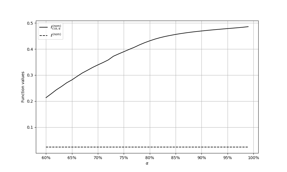
Figure 1: $\ell^{\rm(nom)}_{\rm cce,\alpha}$ vs $\ell^{\rm(nom)}$

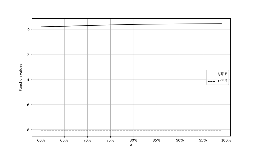
Figure 2: $\ell^{\rm(emp)}_{\rm cce,\alpha}$ vs $\ell^{\rm(emp)}$

The differences are considerable, but sometimes less conservative compared to robust methods, as showcased by the following experiment where we constructed, for each scenario $i=1,\dots,10$, a robust StQP (2) each with the choice of a box uncertainty set of the form

$$\mathcal{U}_{i}=\left\{{\mathsf{U}}={\mathsf{U}}^{\top}:\rho[\underline{{\mathsf{Q}}_{i}}-{\mathsf{Q}}^{\rm(nom)}_{i}]_{k\ell}\leq{\mathsf{U}}_{k\ell}\leq\rho[\overline{{\mathsf{Q}}_{i}}-{\mathsf{Q}}^{\rm(nom)}_{i}]_{k\ell}\mbox{ for all }k,\ell\right\}$$ (11)

where

$$(\underline{{\mathsf{Q}}_{i}})_{k\ell}:=\min_{j}\,({\mathsf{Q}}_{ij})_{k\ell},\quad\quad(\overline{{\mathsf{Q}}_{i}})_{k\ell}:=\max_{j}\,({\mathsf{Q}}_{ij})_{k\ell}$$

defines a box covering all realizations (depending on the instance number $i$), and $\rho\in(0,1]$ is a parameter controlling the size of $\mathcal{U}_{i}$. By application of [4, Theorem 3] to the constructed uncertainty sets $\mathcal{U}_{i}$, we obtain

$$\min_{{\mathbf{x}}\in\Delta} \,\max_{{\mathsf{U}}\in\mathcal{U}_{i}}\,{\mathbf{x}}^{\top}({\mathsf{Q}}_{i}^{\rm(nom)}+{\mathsf{U}}){\mathbf{x}}=\min_{{\mathbf{x}}\in\Delta}\left[{\mathbf{x}}^{\top}{\mathsf{Q}}_{i}^{\rm(nom)}{\mathbf{x}}+\max_{{\mathsf{U}}\in\mathcal{U}_{i}}\,{\mathbf{x}}^{\top}{\mathsf{U}}{\mathbf{x}}\right]$$

$$=\left[\min_{{\mathbf{x}}\in\Delta}\,{\mathbf{x}}^{\top}{\mathsf{Q}}_{i}^{\rm(nom)}{\mathbf{x}}+\rho\,{\mathbf{x}}^{\top}(\overline{{\mathsf{Q}}_{i}}-{\mathsf{Q}}_{i}^{\rm(nom)}){\mathbf{x}}\right]$$

$$=\min_{{\mathbf{x}}\in\Delta}\,{\mathbf{x}}^{\top}[(1-\rho)\,{\mathsf{Q}}_{i}^{\rm(nom)}+\rho\,\overline{{\mathsf{Q}}_{i}}]{\mathbf{x}}\,.$$

We set $\rho=0.8$ and denote by ${\mathbf{x}}_{i}^{\rm(rob)}$ the robust solution obtained from the robust StQPs (2) with uncertainty sets (11). We compare the obtained realized feasible values in a similar way as above, this time observing the differences $\ell^{\rm(nom)}_{\rm rob}-\ell^{\rm(nom)}$ and $\ell^{\rm(emp)}_{\rm rob}-\ell^{\rm(emp)}$ with

$$\ell^{\rm(nom)}_{\rm rob}:=\frac{1}{10}\sum_{i=1}^{10}\mathbf{x}_{i}^{\rm(rob)\top}\mathsf{Q}_{i}^{\rm(nom)}\mathbf{x}_{i}^{\rm(rob)}\quad\mbox{and}\quad\ell^{\rm(emp)}_{\rm rob}:=\frac{1}{1000}\sum_{i=1}^{10}\sum_{j=1}^{100}\mathbf{x}_{i}^{\rm(rob)\top}\mathsf{Q}_{ij}\mathbf{x}_{i}^{\rm(rob)}\,.$$

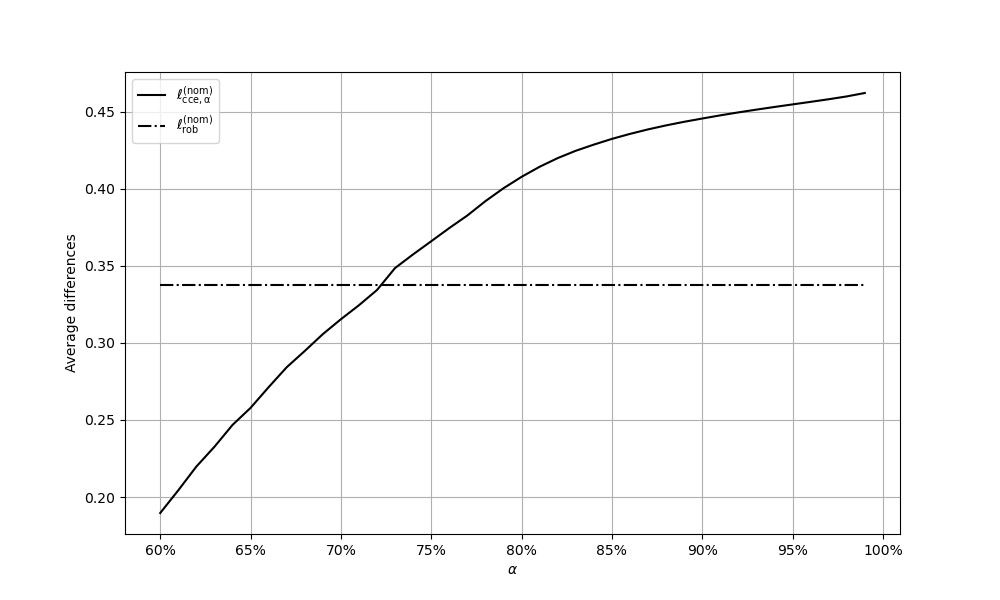
Figure 3: $\ell^{\rm(nom)}_{\rm cce,\alpha}-\ell^{\rm(nom)}$ vs $\ell^{\rm(nom)}_{\rm rob}-\ell^{\rm(nom)}$

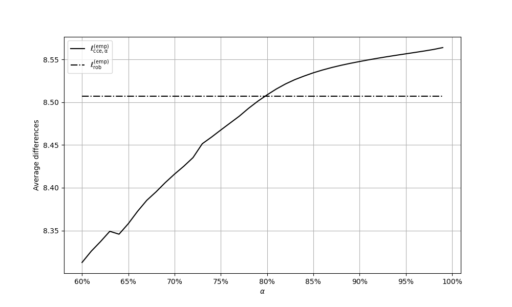
Figure 4: $\ell^{\rm(emp)}_{\rm cce,\alpha}-\ell^{\rm(emp)}$ vs $\ell^{\rm(emp)}_{\rm rob}-\ell^{\rm(emp)}$

6 Conclusion

We introduced and motivated the chance-constrained epigraphic StQP, a new model for solving uncertain StQPs under distributional assumptions, and established a deterministic counterpart as an instance in the same problem class (another StQP). Our findings parallel similar observations on robust StQPs, and indeed a special variant of this model is equivalent to a particular robust formulation. However, preliminary experiments seem to suggest that the chance-constrained epigraphic StQP can be less conservative than a robust approach, if the confidence level (probabilistic optimality guarantee) is not too large.

References

• Aizenman et al. [2017] M. Aizenman, R. Peled, J. Schenker, M. Shamis, and S. Sodin. Matrix regularizing effects of Gaussian perturbations. Communications in Contemporary Mathematics, 19(03):1750028, 2017.
• Bomze [1998] I. M. Bomze. On standard quadratic optimization problems. Journal of Global Optimization, 13:369–387, 1998.
• Bomze et al. [2018] I. M. Bomze, W. Schachinger, and R. Ullrich. The complexity of simple models – a study of worst and typical hard cases for the standard quadratic optimization problem. Mathematics of Operations Research, 43(2):651–674, 2018.
• Bomze et al. [2021] I. M. Bomze, M. Kahr, and M. Leitner. Trust your data or not – StQP remains StQP: Community Detection via Robust Standard Quadratic Optimization. Mathematics of Operations Research, 46:301–316, 2021.
• Bomze et al. [2022] I. M. Bomze, M. Gabl, F. Maggioni, and G. Pflug. Two-stage stochastic standard quadratic optimization. European Journal of Operational Research, 299(1):21–34, 2022.
• El Ghaoui et al. [2003] L. El Ghaoui, M. Oks, and F. Oustry. Worst-case value-at-risk and robust portfolio optimization: A conic programming approach. Operations Research, 51(4):543–556, 2003.
• Geman [1980] S. Geman. A limit theorem for the norm of random matrices. The Annals of Probability, 8(2):252–261, 1980.
• Larsen et al. [2002] N. Larsen, H. Mausser, and S. Uryasev. Algorithms for Optimization of Value-at-Risk, pages 19–46. Springer US, Boston, MA, 2002.
• Linsmeier and Pearson [1996] T. J. Linsmeier and N. D. Pearson. Risk measurement: An introduction to value at risk. Technical Report 96-04, University of Illinois at Urbana-Champaign, IL, 1996.
• Marchenko and Pastur [1967] V. A. Marchenko and L. A. Pastur. Distribution of eigenvalues for some sets of random matrices. Mathematics of the USSR-Sbornik, 1(4):457–483, 1967.
• Markowitz [1952] H. Markowitz. Portfolio selection. The Journal of Finance, 7:77–91, 1952.
• Motzkin and Straus [1965] T. S. Motzkin and E. G. Straus. Maxima for graphs and a new proof of a theorem of Turán. Canadian Journal of Mathematics, 17:533–540, 1965.
• Pavan and Pelillo [2003] M. Pavan and M. Pelillo. Dominant sets and hierarchical clustering. In Proceedings Ninth IEEE International Conference on Computer Vision, pages 362–369. IEEE, 2003.
• Shaked-Monderer and Berman [2021] N. Shaked-Monderer and A. Berman. Copositive and completely positive matrices. World Scientific Publishing Co. Pte. Ltd., Hackensack, NJ, 2021.
• Shapiro and Zarembo [2016] B. Shapiro and K. Zarembo. Level crossing in random matrices: I. Random perturbation of a fixed matrix. Journal of Physics A: Mathematical and Theoretical, 50(4):045201, 2016.
• Silverstein [1985] J. W. Silverstein. The smallest eigenvalue of a large dimensional Wishart matrix. The Annals of Probability, 13(4):1364–1368, 1985.
• Wigner [1958] E. P. Wigner. On the distribution of the roots of certain symmetric matrices. Annals of Mathematics, 67(2):325–327, 1958.