(12.0cm,0cm)RUP-24-21, YITP-24-157
Soliton self-gravity and core-halo relation in fuzzy dark matter halos
Abstract
Fuzzy dark matter (FDM) is an attractive dark matter candidate composed of ultralight particles. In this paper, toward a clear understanding of the core-halo relation in the FDM halos, we consider a simple model of the soliton-halo system, in which the self-gravitating soliton core is formed in the presence of Navarro–Frenk–White (NFW) halo potential as an external field. Solving numerically the Schrödinger-Poisson equation, the self-gravitating soliton is obtained as a ground-state solution, which is characterized by the two key parameters, i.e., size of soliton core and its strength of self-gravity relative to those of the NFW halo. Using our soliton-halo model, we investigate the properties of soliton cores found in cosmological simulation, and the key parameters characterizing these solitons are reconstructed in a self-consistent manner. Results suggest that (1) the soliton core properties depend critically on both the self-gravity of the soliton and the external potential of the host halo, and (2) the scatter observed in the core-halo relation cannot be explained solely by the one in the halo’s concentration-mass relation, as previously suggested, but also significantly influenced by intrinsic features of the soliton core, potentially arising from local dynamics at the halo center. We also demonstrate that the FDM mass can be reconstructed from the simulation data characterizing the halo density profile, providing a basis for applying the model to observational studies.
1 Introduction
The dark matter is the invisible matter component that makes up of the energy contents of the universe. Despite the numerous attempts to detect dark matter directly, its nature remains unknown. In the standard cosmological model, the dark matter is described by the particle with negligible velocity dispersion, referred to as the cold dark matter (CDM). While the CDM paradigm has been successful in explaining the observation on scales larger than galaxies [1, 2], it faces the problem of discrepancy from the observations at small scales (see e.g., refs [3, 4] for review).
One of the attractive alternatives to the CDM is the dark matter described by the ultralight scalar particle with mass eV, often called fuzzy dark matter (FDM) [5]. Since the FDM has a galaxy scale long de Broglie wavelength
| (1.1) |
the wave-like behavior appears at astrophysical scales. It suppresses the small-scale structure, while remains unchanged in the evolution and formation of the large scale structure [6, 7, 8, 9]. In addition, the FDM has strong motivation from the theory beyond the Standard Model of particle physics, as exemplified by axion-like particles predicted by string theory [10, 11, 12]. Therefore, investigating the properties of FDM and observations at small scale can provide opportunities to explore the nature of the dark matter related to unknown physics.
The dynamics and the structure formation of FDM are governed by the Schrödinger equation coupled to the Poisson equation. Numerical simulations of this system have shown that there appear several unique features in the structure of dark matter halos [13, 14]. The density profile has a flat core called soliton core at the central region, with the outer regions resembling those found in a CDM halo, which are well described by the Navarro-Frenk-White (NFW) profile [15, 16]. In particular, early numerical works suggest the universal relation between the configuration of the soliton core and the host halo. It is expressed as the pawer-law behavior of the radius and the mass of the soliton core with respect to the halo mass [14, 17, 18, 19]. However, the core-halo relation of the numerical simulations in different setups does not agree [20]. In addition, there is a large scatter in the core-halo relation even in the same setup of the each simulation, but what cause of the diversity and the scatter has not yet been clarified.
So far, most of the studies has been based on numerical simulations [21, 22, 18, 20, 23, 17, 19, 24, 25, 26, 27], and little analytical work has been done (but see [28, 29, 30]). In order to elucidate the diversity in numerical simulations as well as to understand the physical properties of the core-halo structure, analytical treatment would be helpful. The difficulty in treating the Schrödinger-Poisson system analytically comes from the nonlinearity originated from the self-gravity, and this is also the case even if we consider a stationary spherical system. In ref. [31], the authors, including one of the authors of this paper, presented an analytical description of the soliton core structure, and derived the core-halo relation, ignoring the soliton self-gravity but taking the influence from the gravity sourced by the host halo into account. With this simplification, Schrödinger-Poisson equation is reduced to a linear system, and they succeeded to obtain accurate analytical solutions for the soliton core, which is described by the ground-state wavefunction of the linear Schrodinger equation. As a result, ref. [31] partly reproduces the core-halo relation obtained by numerical simulations. Interestingly, the relation they derived involves an additional factor which crucially depends on the halo concentration. Since the concentration-mass relation is known to exhibit a large scatter in the CDM simulations [32], the authors of ref. [31] suggest that the diversity of the core-halo relation is originated from the scatter in the concentration-mass relation (see ref. [30] for more quantitative discussion).
In this paper, extending the work by ref. [31], we further investigate the soliton core structure and its relation to host halo properties from a simplified setup. In particular, taking the soliton’s self-gravity into account, we critically examineits impact on the the core-halo relation. We consider the FDM halo as a superposition of wavefunctions of the ground-state representing the soliton core and excited states representing the host halo, the latter of which are treated as an external background, and is described by the NFW density profile. Then, the soliton core, described as a ground-state wave function, is characterized by the two key parameters. While one of them is related to the size of the soliton core, another characterizes its strength of self-gravity. Both of them are dimensionless parameters relative to the halo characteristics. In this respect, our soliton-halo system allows us to discuss the core-halo relation more consistently.
Solving numerically the Schrödinger-Poisson equation, the soliton solution is obtained, and comparing it with those found in numerical simulations, the key parameters of the soliton core properties are reconstructed for each halo. The results indicate that most of the FDM halos observed in the simulations lies at the parameter region where both the self-gravity of the soliton core and the host halo are important. Further, the parameter which controls the soliton self-gravity exhibits a large scatter among host halos having the same mass. This seems difficult to explain solely based on the intrinsic properties of halos arising from the concentration-mass relation, in contrast to what has been suggested by refs. [31, 30]. Rather, our results imply that the core-halo relation and its diversity found in numerical simulations are originated not only from the host halo properties, associated with the formation and merger histories, but also from the soliton intrinsic features, perhaps arising from the local dynamics around halo center.
This paper is organized as follows. In section 2, we introduce a model of the soliton core-halo system, in which the self-gravity of the soliton is properly taken into account under the external halo potential. This system is reduced to a stationary problem of the spherically symmetric Schrodinger-Poisson equation, and we show in section 3 that it involves the two limiting cases, in which several properties of the ground-state wavefunction are analytically derived. In section 4, we present the numerical method to solve the introduced Schrödinger-Poisson system, and show the results of the numerical computation. In section 5, the model parameters and the FDM mass are reconstructed from the data of the FDM halo simulations. We discuss the implication of the result of the reconstruction to the core-halo relation. Section 6 is devoted for summary and discussion. For the whole of this paper, we use the notation .
2 Schrödinger-Poisson system
In this section, we introduce an analytical model of the FDM halo. We here write down the Schrödinger-Poisson equations as the basic equations describing the FDM halos. In the comoving coordinate system, they are given by (e.g., [10])
| (2.1) | ||||
| (2.2) |
where is the wavefunction of FDM with the mass . Here, is a scale factor, and is the gravitational potential sourced by the density of FDM
| (2.3) |
2.1 A model of core-halo system
FDM halo simulations based on the Schrödinger-Poisson equation have confirmed the existence of a core-like density profile structure at the center of the halo, known as a soliton core, which has a de Broglie wavelength scale [13, 14, 25, 20]. The soliton core fits well with the ground-state of the stationary spherically symmetric solution of the Schrödinger-Poisson equation. Outside the soliton core, there exist density fluctuation granules of comparable size to the soliton core [13, 14], which are caused by interference of excited states [33]. There are several framework to deal with such a granule structure of the stationary halo based on Schrödinger-Poisson equation (e.g., [34, 35, 36, 33]). To describe the soliton-like core structure at the halo center, one simple approach is to time-average the contribution from these granules, which are represented as a superposition of excited states with non-zero angular momentum. Then, the density profile outside the soliton core is close to the Navarro-Frenk-White (NFW) profile, given by [15, 16].
| (2.4) |
where represents the radial distance from the halo center, and and are constant parameters with the dimensions of density and length.The overall density profile of the FDM halo is thus represented as the sum of the soliton core and the NFW density profile:
| (2.5) |
Since the Poisson equation is linear, the potential is the sum of those originating from and as
| (2.6) |
where and are the solutions of each Poisson equation
| (2.7) | ||||
| (2.8) |
The Poisson equation for the NFW density profile can be solved as
| (2.9) |
We assume the stationary spherical wave function, i.e., with . In this setup, the Schrödinger-Poisson equation can be reduced to the following form:
| (2.10) | ||||
| (2.11) |
The previous work [31] develops an analytical method to investigate the particular case of this equation while neglecting the contribution of soliton self-gravity111To be precise, ref. [31] ignores the soliton self-gravity in their analytical model, but estimate its impact on the soliton core structure based on perturbative treatment. They found that the self-gravity of the soliton is not entirely negligible. .
2.2 Dimensionless equations
To clarify the structure of the Schrödinger-Poisson equation, it is convenient to introduce dimensionless quantities as
| (2.12) | ||||
| (2.13) | ||||
| (2.14) | ||||
| (2.15) |
We also define a dimensionless parameter
| (2.16) |
By applying these variables in eq. (2.10) and eq. (2.11), the dimensionless Schrödinger-Poisson equation is given by
| (2.17) | ||||
| (2.18) |
Since we are interested in the bound state solution of the FDM as mentioned above, we focus on the solution with the regularity at the center and a decaying boundary condition at infinity. In this case, the eigenvalue is discretized. Due to the non-linearity of the self-gravity, the solutions depend on the amplitude of the wavefunction. Here, we introduce a parameter that characterizes the strength of the self-gravity as
| (2.19) |
Therefore, the boundary conditions can be formally written as
| (2.20) | ||||
| (2.21) | ||||
| (2.22) | ||||
| (2.23) | ||||
| (2.24) |
In particular, the central density of the soliton core, , is expressed as
| (2.25) |
3 Analytical properties of soliton-halo system
The setup described in the previous section involves the two dimensionless parameters, and . Depending on the choice of their parameters, the system can be reduced to a more simplified form. In the following, we consider the two limiting cases, i.e., the case where either the background halo potential or the soliton self-gravity is ignored, summarized in Table 1. We derive several key quantities characterizing the conditions for two limiting cases.
3.1 Two limiting cases
3.1.1 Limit A: the case ignoring the external halo potential
Let us first consider the case where the potential of the host halo, described by the NFW profile, is ignored. The Schrödinger-Poisson equations eq. (2.17) and eq. (2.18) are reduced to
| (3.1) | ||||
| (3.2) |
This set of equations is known to be invariant under
| (3.3) |
where the parameter beging a positive real constant [14, 37]. Note that this scaling symmetry is broken when the NFW potential is included beyond the limit A. When is set to 1, i.e., , the ground-state solution can be obtained numerically as and [38]. Thanks to the scaling symmetry, we can construct the solution scaled by an arbitrary constant as
| (3.4) | ||||
| (3.5) |
Also, the dimensionless core radius , defined as the radius at which the soliton density is half of its central value, i.e,
| (3.6) |
is also obtained, and for , the numerical calculations yield . Putting back to the expression with the scaling law, we thus have
| (3.7) |
Recall that the radius is related to the dimensionless quantity through , combining eq. (2.25) with eq. (3.7) leads to the following relation [14]:
| (3.8) |
where and denotes solar mass and parsection
| Dominant potential | Parameter region | Core radius | |
|---|---|---|---|
| Limit A | Soliton core | ||
| Limit B | Host halo |
3.1.2 Limit B: the case ignoring the soliton’s self-gravity potential
Next consider another limiting case, in which we ignore the contribution of the soliton core to the gravitational potential. We call it limit B. This is to drop the second term in the square bracket of the right hand side of eq. (2.17). Then, the Schrödinger-Poisson equations are reduced to the linear Schrödinger system, and the equation to solve becomes
| (3.9) |
Note that this Schrödinger equation is no longer invariant under the scaling transformation eq. (3.3). In ref. [31], applying the uniform asymptotic approximation, the authors obtain the analytical expressions for the eigenfunction of eq. (3.9), which are found to describe very accurately the soliton solutions in the case of . The eigenvalues are then obtained by solving the following transcendental equation:
| (3.10) |
where denotes the Airy function of the first kind, and is defined as
| (3.11) |
with the quantity being the turning point satisfying the relation . Imposing further the condition , it is possible to get a more concise expression for the eigenvalues, and the ground-state eigenvalue is approximately expressed as
| (3.12) |
In ref. [31], taking advantage of the analytical form of the ground-state eigenfunction, the expression of the core radius is also obtained in a simple form. Denoting its dimensionless core radius by , we have
| (3.13) |
with the quantity being the numerical constant, [31]. Substituting eq. (3.12) into the above, a further approximation is obtained:
| (3.14) |
with .
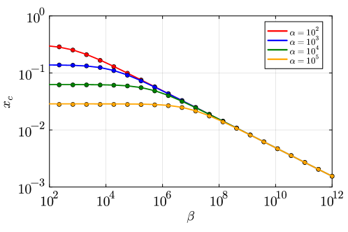
3.1.3 Critical region
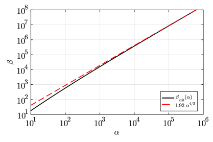
The two limiting cases described in section 3.1.1 and 3.1.2 appear as asymptotic solutions, and in general, the ground-state solution of Schrödinger-Poisson equations eq. (2.17) and eq. (2.18) is neither the limit A nor limit B. Nevertheless, depending on the choice of parameters, one expects that the solution exhibits the behaviors similar to either the limit A or limit B. To clarify the boundary of the regions where the solution is expected to behave like the limit A or B, we introduce the critical value by equating the dimensionless core radius for limit A and B, namely, eq. (3.7) and . Thus, for a given , the critical value is defined as
| (3.15) |
In particular, for the region of , the above expression is simplified by using eq. (3.14)as
| (3.16) |
The ground-state solution is thus expected to behave like the limit A in the region of , while the behavior like the limit B appears in the region of .
Figure 1 illustrates the critical value of . The black solid line shows eq. (3.15) with the quantity being evaluated numerically by solving eq. (3.10). The red dashed line represents the result from the approximate expression of at eq. (3.16), which gives an accurate estimation of the critical value at .
As defined above, the asymptotic behavior of the core radius in terms of with can be expressed as
| (3.17) |
3.2 Core mass
Next, we discuss the core mass, which characterize the core-halo relation. We define the core mass as the enclosed total mass of dark matter within the core radius as
| (3.18) | ||||
| (3.19) | ||||
| (3.20) |
Here, we consider the contributions both from the soliton and the host halo.
In both of the limits A and B, the soliton core density is shown to be well fitted by the formula [14, 31]
| (3.21) |
with the constant setting to , so as to satisfy . Substituting this into eq. (3.19), the soliton core mass recast as
| (3.22) |
where the constant is determined numerically as
| (3.23) |
Further, we rewrite eq. (3.22) with the expression of the dimensionless core radius given at eq. (3.7) in the limit A and at eq. (3.14) in the limit B. We obtain
| (3.24) |
Similarly, substituting the core radius from eq. (3.7) or eq. (3.14) into eq. (3.20), the core mass coming from the host halo contribution is expressed in the two limiting cases as
| (3.25) |
With the expressions given above, we can analytically evaluate which contribution dominates the total core mass.
By assuming , from eqs. (3.20), (3.22), and (2.25), the ratio of the two core masses is given by
| (3.26) |
In the region where the limit A valid , since the core radius is given by eq. (3.7), the ratio of the two core masses is given by
| (3.27) |
From eq. (3.16), in the region where the limit A is valid , the above equation can be evaluated as . Thus, the contribution to the core mass from the soliton density is always larger than from the host halo density. On the other hand, in the region where the limit B is valid , from eqs. (3.14) and (3.26), the ratio of the two core masses is given by
| (3.28) |
If , it results in . Therefore, the contribution to the core mass from the host halo is larger than from the soliton core in the most regions where the limit B is valid .
From the above, the asymptotic behavior of the total core mass for each is given by 222 In the region of the limit B is valid, the Schrödinger-Poisson equation can be approximated as a linear equation, so the amplitude of the density is indeterminate. In ref. [31], the amplitude of the density is determined by substituting eq. (3.14) in eq. (3.8) as (3.29) The formula for the central density eq. (3.8) does not hold in the region where , thus the above derivation of the core mass is not appropriate. Nevertheless, this core mass approximately matches the first formula of eq. (3.31), except for a subtle factor difference. Assuming , the first formula of eq. (3.31) can be approximated as (3.30) Therefore, eqs. (3.29) and (3.30) match except for a factor of around 1.6.
| (3.31) |
In the limit case A, by substituting eqs. (2.16) and (3.7) into the first formula of eq. (3.31), we obtain the scaling law for the core mass
| (3.32) |
3.3 Maximam core radius and minimam core mass
In this model, we can discuss the limits of values that the quantities characterizing the solito core can take. The maximum core radius for a given is given by eq. (3.17) as
| (3.33) |
which corresponds to the limit B. This is because the dimensionless core radius in the limit A is a decreasing function of . On the other hand, the minimum core mass is approximately given by
| (3.34) |
This follows from the numerical verification that, assuming is expressed by equation eq. (3.16), the inequality
holds, at least in . Therefore, the minimum core mass corresponds to the core mass in the region where the limit B is valid .
In the previous subsections, the maximum core radius and the minimum core mass for a given are obtained as eq. (3.33) and eq. (3.34), respectively. However, is a parameter related to the properties of the host halo, as defined by eq. (2.16). As shown in appendix B, when introducing the concentration parameter , the parameters and of the NFW density profile can be considered as variables determined by and the halo mass . Thus,by taking the limit of , the maximum value of and the minimum value of for the given halo mass can be obtained as
| (3.35) | ||||
| (3.36) |
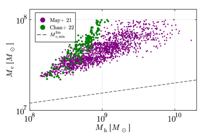
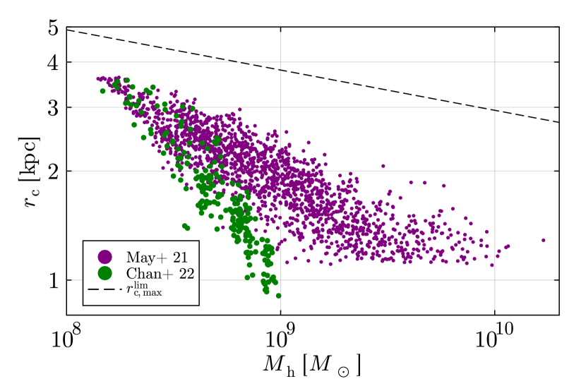
where we have set the reference values of the cosmological parameters as . These equations provide universal upper limits for and lower limits for that are independent of and . In other words, given the FDM mass and halo mass, the core radius does not exceed , and the core mass does not fall below . Therefore, these limits are expected to be useful as criteria for determining the FDM mass from observational data.
4 Numerical analysis
In this section, we present the numerical solutions of the Schrödinger-Poisson equations eq. (2.17) and eq. (2.18). After describing the numerical method in section 4.1, the ground-state solution is numerically obtained for various set of parameters in section 4.2, and the results are compared with the two limiting cases discussed in previous section.
4.1 Method
Here, following ref. [38], we describe the numerical method to find the ground-state eigenfunction of the Schrödinger-Poisson equations eq. (2.17) and eq. (2.18) with the five boundary conditions eq. (2.20)-eq. (2.24). Since it is not practical to implement the boundary condition at infinity in a numerical scheme, we introduce a finite boundary at . This allows us to approximate eq. (2.17) around the large as
| (4.1) |
As a result, is exponentially damped around as
| (4.2) |
Similarly, the right hand side of eq. (2.18) becomes negligible at large , and around the soliton self-gravity potential takes the form
| (4.3) |
We also set a small but nonzero inner boundary to avoid an unexpected divergence at the center. To sum up, We adopt the alternative boundary conditions instead of eq. (2.20)-eq. (2.24) as follows [38]:
| (4.4) | ||||
| (4.5) | ||||
| (4.6) | ||||
| (4.7) | ||||
| (4.8) |
Eigenvalue and eigenstates are obtained numerically by using the shooting method. First, with the initial guess of the values of and , the dimensionless Schrödinger-Poisson equation eq. (2.17) and eq. (2.18) are solved outward from to , where we have set the matching point as . Second, by assuming the value of and , the dimensionless Schrödinger-Poisson equation eq. (2.17) and eq. (2.18) are solved inward from to . The inward and outward solutions generally do not smoothly connect at . The Newton-Rapthon method is then used to find the appropriate values of , , , and , which give , and their derivatives connected at . This process is repeated until the convergence is achieved. In the numerical calculation presented below, we set to . The outer boundary is chosen such that the square of the wavefunction satisfies .
Note that the convergence of the Newton-Raphson method is not always efficient. It becomes extremely slow or to an undesirable excited state if the initial values of are not sufficiently close to the actual values. Therefore, for given parameters , the computations are performed using an iterative method as follows.
-
1.
First, the eigenvalue and the eigenstate of the linearized Schrödinger equation eq. (3.9) are obtained numerically for the parameters , where . In the limit where the soliton self-gravity is neglected (limit B), the Schrödinger equation is reduced to a linear system, as we mentioned in section 3.1.2. Discretizing and replacing the derivatives at each point with finite differences, the linearized Schrödinger equation eq. (3.10) is represented in a matrix form [31]. By diagonalizing this matrix, the eigenvalue and the eigenfunction are determined simultaneously. Then, the dimensionless core radius is obtained from eq. (3.6).
-
2.
Provided the parameters , the Schrödinger-Poisson equations eq. (2.17) and eq. (2.18) are next solved by using the shooting method and the Newton-Raphson method. The initial condition for the eigenvalue is set to the value obtained in step 1. The initial condition for is obtained by integrating the Poisson equation with eq. (3.21) to give
(4.9) with obtained in step 1. The initial conditions for both and are set to 0.
-
3.
Choosing the value of slightly larger than , the Schrödinger-Poisson equations eq. (2.17) and eq. (2.18) are solved for the new parameter set , again using the shooting method and the Newton-Raphson method, with the initial guess of obtained in the previous step. We gradually increase the value of , and repeat this step until we reach at the desired value of .
4.2 Results
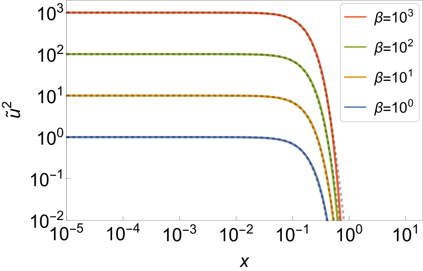
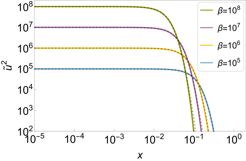
With the numerical methods described above, the ground-state wavefunction , the self-gravitational potential , and the eigenvalue are simultaneously and uniquely determined for given parameters . Figure 2 shows the examples of the dimensionless soliton density obtained by the above numerical method. The fitting formula of the soliton density profile in eq. (3.21), depicted as gray dashed lines, fits well with the soliton profiles obtained from the numerical calculation, regardless of the value of the parameters . As illustrated in the left panel of figure 2, which corresponds to the cases where the host halo potential is dominant, the core radii do not depend on , consistent with eq. (3.14). In contrast, the right panel of figure 2 presents the results where the soliton self-gravity potential is dominant, and manifests the dependence of the core radius on , again consistent with eq. (3.7).
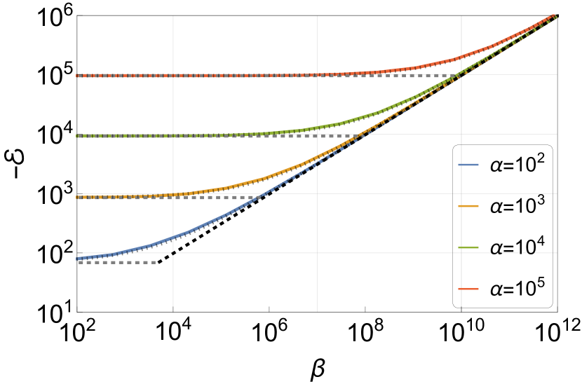
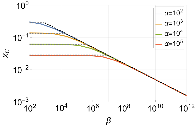
Figure 3 presents the numerical values of the dimensionless ground-state eigenvalue (left) and the core radius (right), plotted as a function of . Each line corresponds to a different value of . As illustrated in the left panel of figure 3, in the region where , the eigenvalue remains constant regardless of the value of , and fits well with the approximate expression at eq. (3.12). On the other hand, in the region where , it fits well with eq. (3.5) regardless of the value of . Combining them, we find that the energy eigenvalue of our model can be well reproduced by the sum of eq. (3.5) and eq. (3.12), given by (see black dotted lines):
| (4.10) |
which still provides a reosonable approximation at the intermediate region .
The right panel of figure 3 shows the dimensionless core radius given as a function of for representative values of . The solid lines represent the results of the numerical calculations, while the gray and black dashed lines represent the dimensionless core radius in the limit A and B, given respectively at eq. (3.7) and eq. (3.14). The asymptotic behaviors of the numerical results match the analytical expressions in the limit A, eq. (3.7) and B, eq. (3.14).
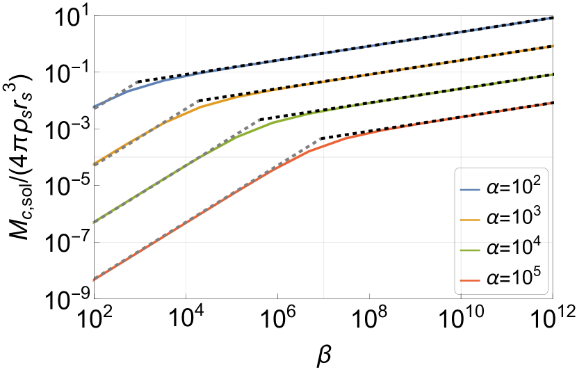
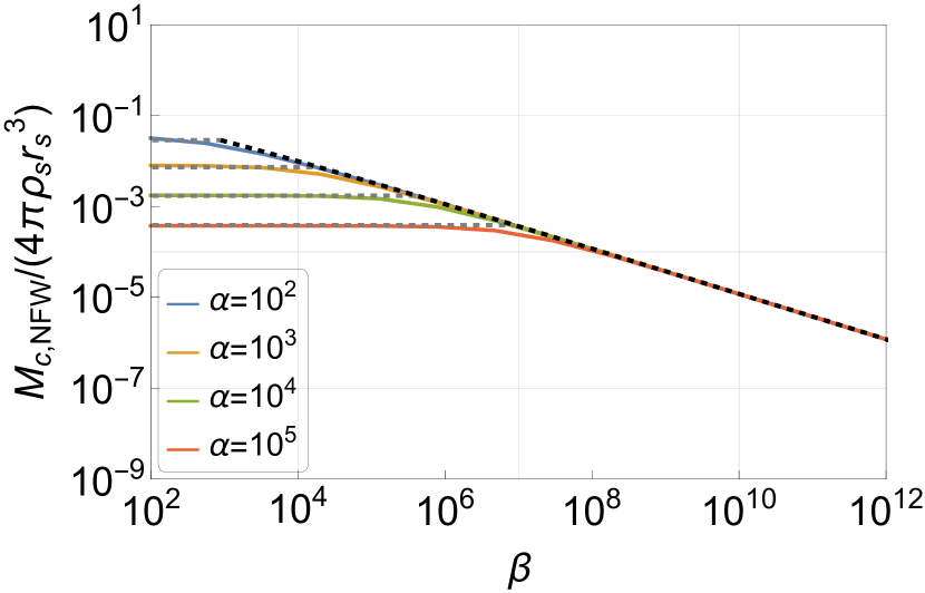
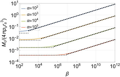
In Figure 4, we also show the core mass of soliton core and the core mass of the NFW density , which are defined by eq. (3.19) and eq. (3.20), respectively. Solid lines represent the results of numerical calculations. The gray and black dashed lines represent the asymptotic results in the limit B, eq. (3.24) and in the limit A, eq. (3.25), respectively.
5 Parameter reconstruction and implication from simulation data
In this section, as an implication of our model of the core-halo system discussed in the previous sections, we apply the model predictions to the solitons found in the numerical simulations of refs. [25] and [20], and interpret their structural properties in relation to the characteristics of the host halos. Specifically, we compare the characteristics of each soliton in numerical simulations with the predictions of the core-halo model to derive the key parameters and the concentration parameter of the host halo, , which are not directly measured from simulations. In section 5.1, we begin by describing the method to reconstruct parameters , , and . Then, in section 5.2, reconstructed results from the simulation data are presented, and statistical properties of the core-halo structure is discussed. In section 5.3, we will briefly show that the FDM mass can be also reconstructed from the dataset in the simulation.
5.1 Formulation of the parameter reconstruction
Let us recall that for a given set of the parameters , togerther with the host halo characteristics such as virial mass and the concentration parameter (or scale radius ), the model of the core-halo system can predict the soliton core characteristics such as core radius , core density , and core mass from the ground-state solution of the Schrödinger-Poisson equations, eq. (2.17) and eq. (2.18) in a fixed cosmological model. Combining the background halo profile, we can also obtain the total halo density profile, given as the sum of the soliton and the NFW profile. Conversely, we can read off the parameter for each soliton from the halo and soliton characteristics, and one can investigate the actual properties of the core-halo system in numerical simulations.
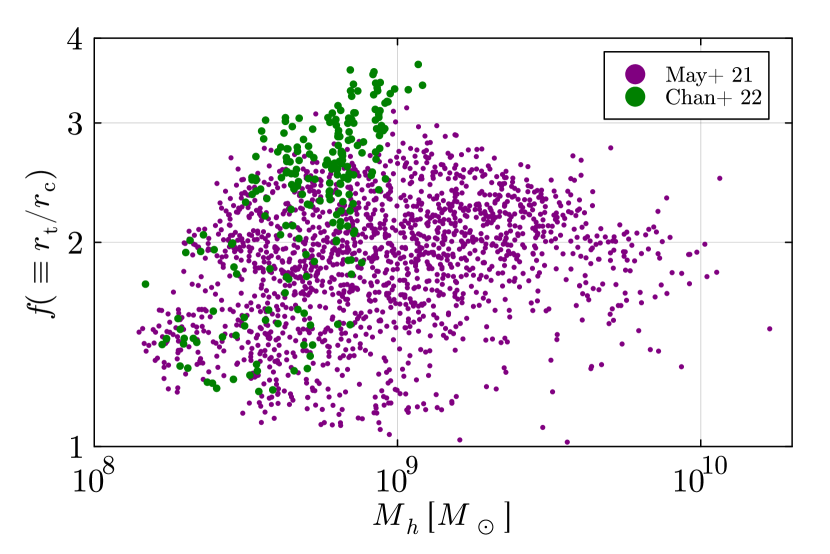
Here, we use the data presented in ref. [20], consisting of the results obtained from soliton merger simulations and simulations started from the cosmological initial condition in ref. [25]. To be precise, we use the measured results of the soliton core radius , transition radius of the total profile , and the halo mass , as shown in figure 5. The transition radius is defined as the scale where the density profile changes from a cored inner profile to the outer NFW profile. Specifically, in ref. [20], the transition radius is determined by fitting the measured halo profile to the analytical fitting form consisting of the inner soliton profile at (eq. (3.21)) and the outer NFW profile at (eq. (2.4))333In determining the transition radius , ref. [20] assumes the relation at eq. (3.8), which is strictly valid in the limit A case. However, as shown in appendix C, our reconstructed reproduce well the scaling relation with , which is derived from eq. (3.8) (see eq. (3.32)). In this respect, the results are self-consistent. .
Given a set of parameters , the method to reconstruct the parameters and is given as follows. Suppose that the cosmological model and the mass of FDM are a priori known444In the reconstructed procedure, the cosmological parameters are fixed as , and FDM mass is fixed as .. eq. (2.16) implies that for a given halo mass, the parameter is given as a single-variate function of the concentration parameter, 555The characteristic density and scale radius are rewritten with and through eq. (B.1) and eq. (B.2), respectively. . Also, the parameter is expressed as a function of by using the definition of the transition radius. From eq. (2.25), the relation leads to
| (5.1) |
with . Substituting the information obtained from simulations into the right-hand side (i.e., , and ), the expression of above is shown to be dependent only on the concentration parameter . Once the parameters and are specified with , our soliton-halo model predicts the dimensionless core radius, , from which the core radius in physical units is computed from
| (5.2) |
Since the core radius is now entirely determined by the single parameter , we can compare it with the measured value of in simulations to derive a consistent estimate of . This, in turn, allows us to determine the parameters and .
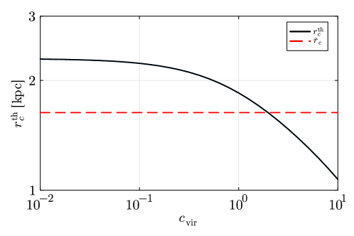
Figure 6 demonstrates how one can obtain a consistent value of for a specific halo. The solid curve represents eq. (5.1) predicted based on the soliton-halo model, and the horizontal dashed line is the core radius measured in simulations. The intersection of these curves gives the solution we want, and from this consistent value of we can reconstruct and for each halo from eqs. (2.16) and (5.1), respectively.
The reconstruction method described above is reduced to a single-parameter search, and as a bybroduct, we also obtain the concentration parameter for each halo, which is not actually presented in ref. [20]. In this respect, one can investigate both the soliton core and halo properties in the FDM model. While this approach would enable an efficient parameter search, it requires solving the Schrödinger-Poisson equations multiple times to compute the dimensionless core radius . In appendix A, to accelerate the parameter reconstruction, we build an accurate fitting formula for , and use it to evaluate the core radius in eq. (5.1).
5.2 Results
5.2.1 Results of the parameter reconstruction
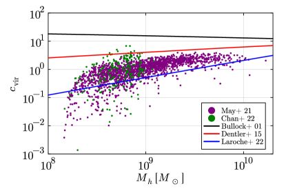
Let us first look at the reconstructed parameters given as a function of host halo mass, . In figure 7, the purple and green dots represent the reconstruction results from the cosmological simulation and soliton merger simulation, respectively. In the data set we used, the soliton merger simulation tends to have a larger scatter than the cosmological simulation.
In figure 7(a), all of the reconstructed concentration parameter are found to be smaller than the one expected from CDM halos [32], depicted as black solid line. This is anticipated, to some extent, from the suppressed growth of small-scale structure with a large de Broglie wavelength. As a result, most of the reconstructed values lie between the two model prediction for FDM halos [39] and [40], which are constructed by multiplying the suppression factor by the concentration-mass relation for CDM halos in ref. [32]. The results indicate that the outer density profile of host halos is mostly dominated by a single power-law with the slope of .
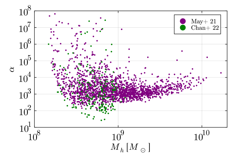
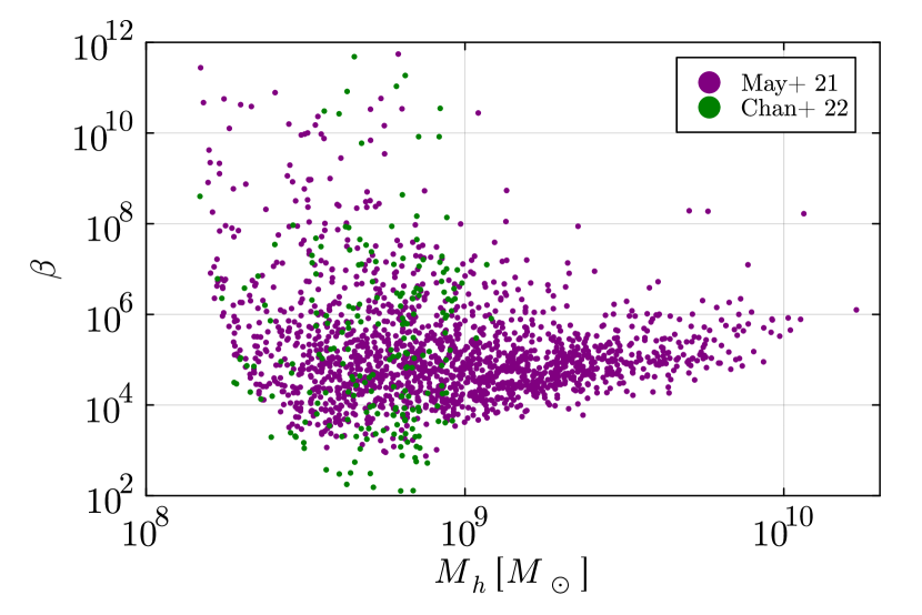
On the other hand, figure 7(b) and 7(c) respectively show the halo mass dependence of the reconstructed parameters and . We see a large scatter in both of the parameters. Especially for host halos of M⊙, the reconstructed results of and can reach a rather large value, and , respectively, although they are not abundant but rather rare.
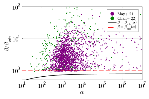
Figure 8 shows the relationship between the reconstructed parameters and , with normalized by the critical value, , defined at eq. (3.16). The black line represents the , which represents the minimum necessary for the existence of the transition radius for each 666The is defined through eq. (5.1), which is recast as (5.3) where . For a given set of parameters and , this equation can be viewed as the transcendental equation for . While this in general gives multiple solutions, the solution for becomes single-valued for specific parameters and , the latter of which is then defined as . . The reconstructed results for satisfy , as all simulated halos have a transition radius. Overall, there is no strong correlation between and , but most cases found in numerical simulations fall within the range , with the parameter ranging from 1 to . This suggests that the self-gravity of the soliton core plays a crucial role in forming the cored density profile of the entire halo system, but the external contribution from the host halo to the soliton core cannot be completely ignored. In other words, the simulated core-halo system lies in between the limit A and limit B, rather than at either extreme.
5.2.2 Scatters in concentration parameter and transition radius
In what follows, we focus only on the reconstructed results from the cosmological simulation since it contains a sufficient amount of data to analyze.
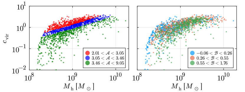
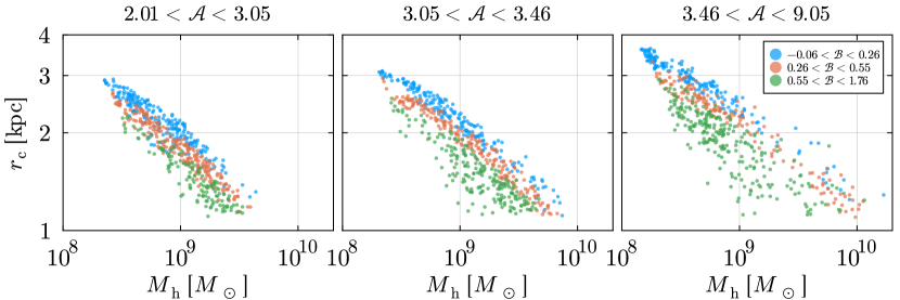
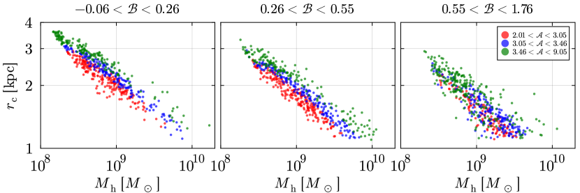
Figures 9 and 10 show the relation between and the host halo mass . The colors of each point represent the value of the reconstructed dimensionless parameters and , where indicates the magnitude of the self-gravity of the soliton core relative to that of the host halo. The reconstructed values of and are divided into three bins so that each bin has the same number of data in each of the left and right panels.
In figure 9, we see that the concentration-mass relation is strongly correlated with , while no clear trend is observed with . This is understood explicitly from eq. (2.16), eq. (B.1), and eq. (B.2). We obtain
| (5.4) |
That is, a high-concentration halo tends to have a smaller value of . Also, low-mass halos tend to have a small concentration parameter, consistent with figure 9.
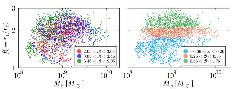
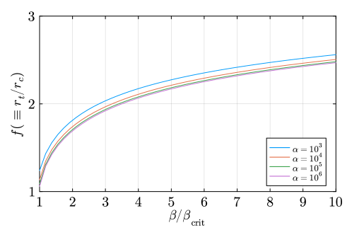
On the other hand, figure 10 shows the relationship between and . Here, each point is classified based on the dimensionless parameters (left) and (right), which are divided into three bins and represented by different colors. These plots show that is strongly correlated with , but has no clear correlation with . These trends can be understood qualitatively from figure 11, where we see clearly the monotonic increase of with , while its increase is hardly changed with .
5.2.3 Scatter in core-halo relation
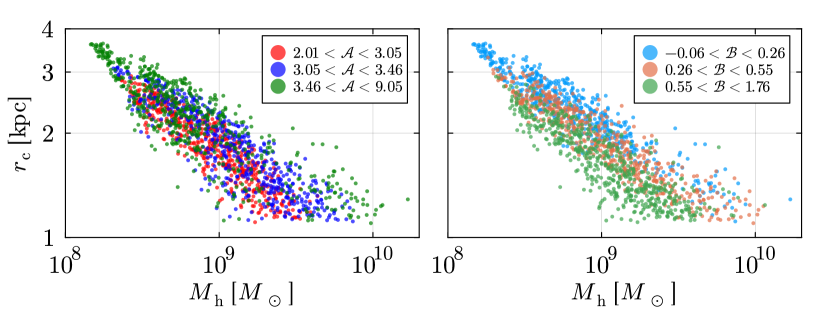
Figure 12 shows the relationship between and classified with (left) and (right) by three different colors. The left and right panels suggest a trend where the core radius tends to decrease as decreases or increases, although these trends appear subtle. To clarify the trend in more comprehensive way, we further classify the relation between and both with and , as shown in figure 13. In other words, the scatter in the core-halo relation is closely related to the scatter in both and .
As discussed in the previous section, given that and correlate with and , respectively, figure 13 suggests that the scatter in the core-halo relation originates from the scatter in both and . In other words, this implies that the scatter in the core-halo relation is due to the unique characteristics of both the halo and the soliton.
Previous research has examined whether the scatter in the core-halo relationship can be explained by the scatter in in N-body simulations of halos, which originates from the history of halo merging and mass accretion [31, 30]. Our results suggest that the scatter in the core-halo relation arises not only from the halo’s merger and mass accretion history but also from the local formation and evolution history of the soliton at the halo center.
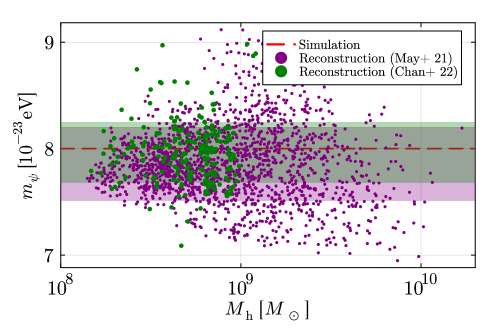
5.3 FDM mass reconstruction
We have so far investigated the properties of the parameters , and from the dataset in the simulation results. In this subsection, as a possible application of the present core-halo model to observational studies, we allow the FDM mass to be free, and demonstrate that by adding the core mass as an additional input, the mass can be estimated in a self-consistent manner using a procedure almost identical to the one presented in section 5.1.
By fixing the halo mass and cosmological parameters, and are determined solely by . Thus, when the FDM mass is a free parameter, can be regarded as a function of and , form its definition eq. (2.16). Similarly, from eq. (5.1), also becomes a function of and . Therefore, the core radius in eq. (5.2) can be extended as
| (5.5) |
From eq. (3.18), the core mass is also calculated from and with given as
| (5.6) |
where we have used eqs. (2.25) and (3.22). The conditions for consistency with the input dataset are and . For a given set of , by solving these equations, and are reconstructed, and they uniquely determine the NFW parameters and as well as the model parameters and . Note that the input parameters used for the reconstructuction are those characterizing the total density profile of each halo. One thus expects that the method presented here can work well for the observations of dwarf spheroidal galaxies, where the information on the halo density profile is obtained through the Jeans analysis from the stellar velocity dispersion data.
We examine the reconstruction method described above using a root finding algorism, where the initial conditions to search for solutions are set to the reconstructed value for (see section 5.2) and the fiducial value in simulations for the FDM mass, i.e., . As a result, the reconstructed values of , and show no significant differences compared to those in figure 7. The estimated FDM mass is shown in figure 14, where we see a good agreement with the fiducial value in the simulation to within about 10% accuracy.
Note that there are observational works that ignore the host halo contribution to the soliton core structure, and obtain the constraint on the FDM mass (e.g. [41, 42]). We can perform the reconstruction of the FDM mass in a similar setup, restricting our core-halo model to the Limit A. In this case, can be reconstructed by substituting the simulation results into eq. (3.32). Comparing these results with those obtained in figure 14, we found that the reconstructed mass differs by only . This suggests that the scaling relation in eq. (3.32), which ignores the contribution of the host halo, serves as a good approximation for the range of parameters we considered, despite the presence of solitons in the simulation results where .
6 Summary and discussion
In this paper, we consider a model of the core-halo system in the FDM cosmology, described by the Schödinger-Poisson equation. In this system, the soliton core is supported by both a self-gravity of the soliton core itself and the host halo under the spherical and stationary ansatz. This system is characterized by the two dimensionless parameters , respectively given at eq. (2.16) and eq. (2.19). In regions where , the limit that ignores the self-gravity of the host halo (limit A) is valid, while, in regions where , the limit that ignores the soliton self-gravity (limit B) is valid. For a given , there exists a maximum value of the core radius and a minimum value of the core mass which correspond to the limit B. These values depend only on the FDM mass and the halo mass, and the concentration parameter through . As shown in section 3.3, the limit for a given FDM mass and halo mass gives the maximum value of and the minimum value of , namely, they are universal bounds for a given FDM mass and halo mass, which are independent of neither nor . These results are expected to be useful as a criterion for determining the FDM mass from observational data.
In addition, we have demonstrated that the dimensionless parameters and can be reconstructed from the set of data in the results of the FDM halo simulations. As a result, most of the solitons in the FDM halo simulations are in the parameter range of . This suggests that the soliton of the FDM halo is not only affected by the self-gravity of the soliton core itself, but also by that of the host halo. Further, the model parameters and are strongly correlated with and , respectively. Thus, it is suggested that the core-halo relation of the FDM halo depends on both the soliton characteristics, such as transition radius and core radius, and the host halo characteristics, such as the concentration parameter. We have also demonstrated that the FDM mass can be also reconstructed from and . This method will be useful to get the constraint on FDM mass by applying the actual data in the future work.
As a final remark, our model can also be applied to investigate the baryonic effects on the soliton core by substituting the NFW density profile with the baryonic profile. In the context of self-interacting dark matter, it is known that baryonic effects contribute to the diversity of rotation curves in spiral galaxies [43]. However, the influence of baryons on the halo structure in FDM remains poorly understood (but see ref. [27]), presenting an important direction for future research.
Appendix A Fitting formula of the dimensionless core radius
In the process of reconstruction in section 5, in eq. (5.2) can be calculated numerically using the shooting method, as demonstrated in the previous section. However, this numerical calculation have been found to be a bottleneck of the calculation time. Therefore, in the following section, we apply a fitting formula for the core radius as
| (A.1) | ||||
| (A.2) |
The constant was set to to match the numerical calculations. The solid line in figure 15 represents this fitting formula eq. (A.1), and the points represent the results of the numerical calculations using the shooting method.
Appendix B Concentration parameter
We introduce the concentration parameter to describe a NFW-type host halo. Here, denotes the virial radius of the NFW density profile. The concentration parameter allows us to express and as
| (B.1) | ||||
| (B.2) |
where is the NFW halo tail mass, and is the present matter density. Here, is the redshift-dependent factor defined as
| (B.3) |
Here, is the matter density parameter at the scale factor .
A concentration-mass relation depends on several factors such as the dark matter model, the initial power spectrum, cosmological parameters, redshift, and so on. While the concentration-mass relation for the CDM halo is numerically well studied by N-body simulations (for example [32]), that for the FDM is relatively poorly understood, except for some analytical models [39, 40].
Appendix C Consistency check with the reconstructed core mass
In section 5 we show how to reconstruct the model parameters and from given simulation results . In our procedure, the core mass is not used as an input parameter because is related to [20].
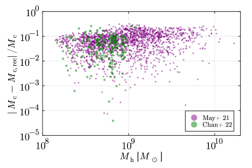
In our model, the core mass can be calculated from the reconstructed parameters and the input parameters from eqs. (3.18)-(3.21). Therefore, the reconstructed core mass can be used as a consistency check by comparing it with the core mass obtained from the simulation results. Figure 16 shows the relative difference between the core mass from the simulation results and the reconstructed core mass, showing that the core mass is correctly reconstructed up to error.
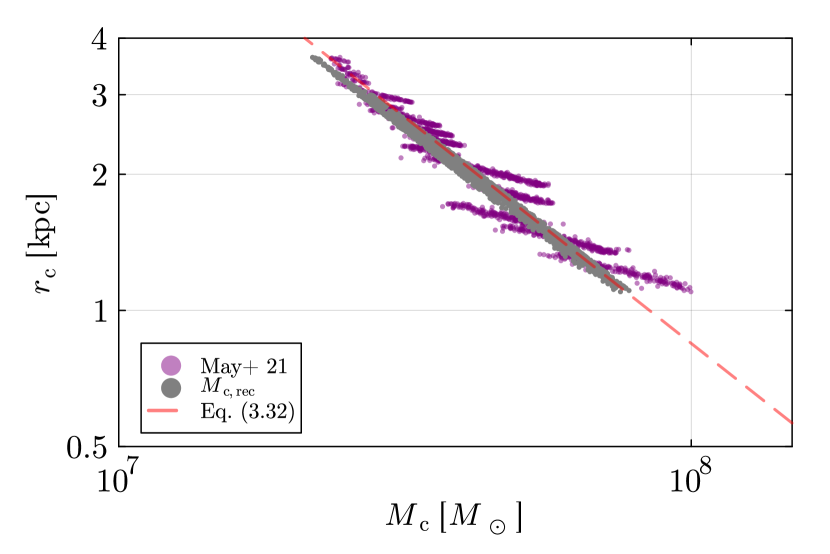
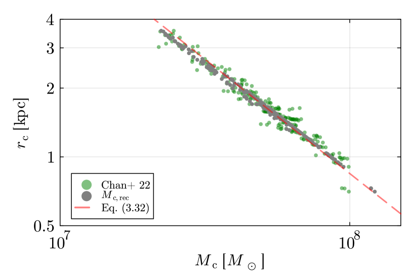
In addition, figure 17 illustrates the relationship between core mass and core radius. The purple and green dots represent the core masses obtained from the cosmological and soliton merger simulations, respectively [25, 20]. The gray dots show the relation between and the reconstructed core mass . Both the simulation and the reconstruction core masses seem to fit well with the scaling relation eq. (3.32) expressed by the red dashed line.
Acknowledgments
We thank Hei Yin Jowett Chan for sharing the data of the FDM simulation results. We thank Takahiro Nishimichi, Elisa Ferreira, Neal Dalal, and Hiroki Kawai for their helpful discussion. Research at Perimeter Institute is supported in part by the Government of Canada through the Department of Innovation, Science and Economic Development and by the Province of Ontario through the Ministry of Colleges and Universities. This work was supported by Japan Society for the Promotion of Science (JSPS) Overseas Research Fellowships (Y.M.), JSPS KAKENHI Grant Number JP23KJ1214 (T.T.) and MEXT/JSPS KAKENHI Grants No. JP20H05861 and No. JP21H01081 (A.T.).
References
- [1] S. Chabanier, M. Millea and N. Palanque-Delabrouille, Matter power spectrum: from Ly forest to CMB scales, Mon. Not. Roy. Astron. Soc. 489 (2019) 2247 [1905.08103].
- [2] SDSS collaboration, The 3-D power spectrum of galaxies from the SDSS, Astrophys. J. 606 (2004) 702 [astro-ph/0310725].
- [3] J.S. Bullock and M. Boylan-Kolchin, Small-Scale Challenges to the CDM Paradigm, Ann. Rev. Astron. Astrophys. 55 (2017) 343 [1707.04256].
- [4] S. Tulin and H.-B. Yu, Dark Matter Self-interactions and Small Scale Structure, Phys. Rept. 730 (2018) 1 [1705.02358].
- [5] W. Hu, R. Barkana and A. Gruzinov, Cold and fuzzy dark matter, Phys. Rev. Lett. 85 (2000) 1158 [astro-ph/0003365].
- [6] J.C. Niemeyer, Small-scale structure of fuzzy and axion-like dark matter, 1912.07064.
- [7] L. Hui, Wave Dark Matter, Ann. Rev. Astron. Astrophys. 59 (2021) 247 [2101.11735].
- [8] E.G.M. Ferreira, Ultra-light dark matter, Astron. Astrophys. Rev. 29 (2021) 7 [2005.03254].
- [9] L. Hui, J.P. Ostriker, S. Tremaine and E. Witten, Ultralight scalars as cosmological dark matter, Phys. Rev. D 95 (2017) 043541 [1610.08297].
- [10] D.J.E. Marsh, Axion Cosmology, Phys. Rept. 643 (2016) 1 [1510.07633].
- [11] P. Svrcek and E. Witten, Axions In String Theory, JHEP 06 (2006) 051 [hep-th/0605206].
- [12] A. Arvanitaki, S. Dimopoulos, S. Dubovsky, N. Kaloper and J. March-Russell, String Axiverse, Phys. Rev. D 81 (2010) 123530 [0905.4720].
- [13] H.-Y. Schive, T. Chiueh and T. Broadhurst, Cosmic Structure as the Quantum Interference of a Coherent Dark Wave, Nature Phys. 10 (2014) 496 [1406.6586].
- [14] H.-Y. Schive, M.-H. Liao, T.-P. Woo, S.-K. Wong, T. Chiueh, T. Broadhurst et al., Understanding the Core-Halo Relation of Quantum Wave Dark Matter from 3D Simulations, Phys. Rev. Lett. 113 (2014) 261302 [1407.7762].
- [15] J.F. Navarro, C.S. Frenk and S.D.M. White, The Structure of cold dark matter halos, Astrophys. J. 462 (1996) 563 [astro-ph/9508025].
- [16] J.F. Navarro, C.S. Frenk and S.D.M. White, A Universal density profile from hierarchical clustering, Astrophys. J. 490 (1997) 493 [astro-ph/9611107].
- [17] M. Nori and M. Baldi, Scaling relations of fuzzy dark matter haloes – I. Individual systems in their cosmological environment, Mon. Not. Roy. Astron. Soc. 501 (2021) 1539 [2007.01316].
- [18] P. Mocz, M. Vogelsberger, V.H. Robles, J. Zavala, M. Boylan-Kolchin, A. Fialkov et al., Galaxy formation with BECDM – I. Turbulence and relaxation of idealized haloes, Mon. Not. Roy. Astron. Soc. 471 (2017) 4559 [1705.05845].
- [19] M. Nori, A.V. Macciò and M. Baldi, Fuzzy Aquarius: evolution of a Milky-way like system in the Fuzzy Dark Matter scenario, Mon. Not. Roy. Astron. Soc. 522 (2023) 1451 [2210.08022].
- [20] H.Y.J. Chan, E.G.M. Ferreira, S. May, K. Hayashi and M. Chiba, The diversity of core–halo structure in the fuzzy dark matter model, Mon. Not. Roy. Astron. Soc. 511 (2022) 943 [2110.11882].
- [21] B. Schwabe, J.C. Niemeyer and J.F. Engels, Simulations of solitonic core mergers in ultralight axion dark matter cosmologies, Phys. Rev. D 94 (2016) 043513 [1606.05151].
- [22] X. Du, C. Behrens, J.C. Niemeyer and B. Schwabe, Core-halo mass relation of ultralight axion dark matter from merger history, Phys. Rev. D 95 (2017) 043519 [1609.09414].
- [23] M. Mina, D.F. Mota and H.A. Winther, Solitons in the dark: First approach to non-linear structure formation with fuzzy dark matter, Astron. Astrophys. 662 (2022) A29 [2007.04119].
- [24] S. Elgamal, M. Nori, A.V. Macciò, M. Baldi and S. Waterval, No Catch-22 for Fuzzy Dark Matter: testing substructure counts and core sizes via high-resolution cosmological simulations, 2311.03591.
- [25] S. May and V. Springel, Structure formation in large-volume cosmological simulations of fuzzy dark matter: impact of the non-linear dynamics, Mon. Not. Roy. Astron. Soc. 506 (2021) 2603 [2101.01828].
- [26] J. Veltmaat, J.C. Niemeyer and B. Schwabe, Formation and structure of ultralight bosonic dark matter halos, Phys. Rev. D 98 (2018) 043509 [1804.09647].
- [27] J. Veltmaat, B. Schwabe and J.C. Niemeyer, Baryon-driven growth of solitonic cores in fuzzy dark matter halos, Phys. Rev. D 101 (2020) 083518 [1911.09614].
- [28] P.-H. Chavanis, Derivation of the core mass – halo mass relation of fermionic and bosonic dark matter halos from an effective thermodynamical model, Phys. Rev. D 100 (2019) 123506 [1905.08137].
- [29] V. Desjacques and A. Nusser, Axion core–halo mass and the black hole–halo mass relation: constraints on a few parsec scales, Mon. Not. Roy. Astron. Soc. 488 (2019) 4497 [1905.03450].
- [30] H. Kawai, A. Kamada, K. Kamada and N. Yoshida, Modeling the core-halo mass relation in FDM halos, 2312.10744.
- [31] A. Taruya and S. Saga, Analytical approach to the core-halo structure of fuzzy dark matter, Phys. Rev. D 106 (2022) 103532 [2208.06562].
- [32] J.S. Bullock, T.S. Kolatt, Y. Sigad, R.S. Somerville, A.V. Kravtsov, A.A. Klypin et al., Profiles of dark haloes. Evolution, scatter, and environment, Mon. Not. Roy. Astron. Soc. 321 (2001) 559 [astro-ph/9908159].
- [33] T.D. Yavetz, X. Li and L. Hui, Construction of wave dark matter halos: Numerical algorithm and analytical constraints, Phys. Rev. D 105 (2022) 023512 [2109.06125].
- [34] X. Li, L. Hui and T.D. Yavetz, Oscillations and Random Walk of the Soliton Core in a Fuzzy Dark Matter Halo, Phys. Rev. D 103 (2021) 023508 [2011.11416].
- [35] J.L. Zagorac, I. Sands, N. Padmanabhan and R. Easther, Schrödinger-Poisson solitons: Perturbation theory, Phys. Rev. D 105 (2022) 103506 [2109.01920].
- [36] S.-C. Lin, H.-Y. Schive, S.-K. Wong and T. Chiueh, Self-consistent construction of virialized wave dark matter halos, Phys. Rev. D 97 (2018) 103523 [1801.02320].
- [37] I.M. Moroz, R. Penrose and P. Tod, Spherically symmetric solutions of the Schrodinger-Newton equations, Class. Quant. Grav. 15 (1998) 2733.
- [38] D.J.E. Marsh and A.-R. Pop, Axion dark matter, solitons and the cusp–core problem, Mon. Not. Roy. Astron. Soc. 451 (2015) 2479 [1502.03456].
- [39] M. Dentler, D.J.E. Marsh, R. Hložek, A. Laguë, K.K. Rogers and D. Grin, Fuzzy dark matter and the Dark Energy Survey Year 1 data, Mon. Not. Roy. Astron. Soc. 515 (2022) 5646 [2111.01199].
- [40] A. Laroche, D. Gilman, X. Li, J. Bovy and X. Du, Quantum fluctuations masquerade as halos: Bounds on ultra-light dark matter from quadruply-imaged quasars, 2206.11269.
- [41] M. Safarzadeh and D.N. Spergel, Ultra-light Dark Matter is Incompatible with the Milky Way’s Dwarf Satellites, 1906.11848.
- [42] K. Hayashi, E.G.M. Ferreira and H.Y.J. Chan, Narrowing the Mass Range of Fuzzy Dark Matter with Ultrafaint Dwarfs, Astrophys. J. Lett. 912 (2021) L3 [2102.05300].
- [43] A. Kamada, M. Kaplinghat, A.B. Pace and H.-B. Yu, How the Self-Interacting Dark Matter Model Explains the Diverse Galactic Rotation Curves, Phys. Rev. Lett. 119 (2017) 111102 [1611.02716].