Exploiting Boosting in Hyperdimensional Computing for Enhanced Reliability in Healthcare
Abstract
Hyperdimensional computing (HDC) enables efficient data encoding and processing in high-dimensional spaces, benefiting machine learning and data analysis. However, underutilization of these spaces can lead to overfitting and reduced model reliability, especially in data-limited systems—a critical issue in sectors like healthcare that demand robustness and consistent performance. We introduce BoostHD, an approach that applies boosting algorithms to partition the hyperdimensional space into subspaces, creating an ensemble of weak learners. By integrating boosting with HDC, BoostHD enhances performance and reliability beyond existing HDC methods. Our analysis highlights the importance of efficient utilization of hyperdimensional spaces for improved model performance. Experiments on healthcare datasets show that BoostHD outperforms state-of-the-art methods. On the WESAD dataset, it achieved an accuracy of , surpassing Random Forest, XGBoost, and OnlineHD. BoostHD also demonstrated superior inference efficiency and stability, maintaining high accuracy under data imbalance and noise. In person-specific evaluations, it achieved an average accuracy of , outperforming other models. By addressing the limitations of both boosting and HDC, BoostHD expands the applicability of HDC in critical domains where reliability and precision are paramount.
I Introduction
Hyperdimensional computing (HDC) is a rapidly advancing field within artificial intelligence, offering numerous valuable qualities that apply to various areas. HDC’s ability to efficiently encode and process data in high-dimensional spaces has generated substantial interest, particularly in machine learning and data analysis [1, 2, 3]. As we contemplate the practical use of HDC-based models in real-world applications, we encounter crucial requirements beyond mere accuracy. These requirements encompass robustness, reliability, consistency, and resource efficiency [4]. Despite these requirements, analyses of HDC in high-dimensional spaces has not yet been fully explored which can lead to overfitting by selecting very high dimension above only performance [5]. Our research shows that the partitioning of high-dimensional spaces directly correlates with the utility of the space, fulfilling those requirements under certain condition.
Meeting the requirements of HDC is anticipated to significantly expand its applicability across various domains, particularly in fields where reliability and precision are paramount, such as healthcare [6, 7]. In addressing healthcare datasets, our evaluation focuses on critical issues such as robustness to noise, consistency in performance, and stability that are non-negotiable for the successful application of HDC in healthcare.
Ensemble methods have been recognized for their ability to prevent overfitting and achieve enhanced performance and stability in predictive modeling [8]. Among these methods, boosting stands out for its capability to aggregate the predictions of multiple weak learners into a robust and accurate ensemble model. The strengths of boosting encompass significant accuracy improvements, resistance to overfitting, versatility across a wide range of machine learning tasks. However, boosting‘s ability across sensitivity to noisy data, performance and stability is dependent on the ability of weak learner. The computational demands of training boosting ensembles can also present challenges in scenarios requiring real-time responses or operating under resource constraints. Furthermore, the overall performance of the ensemble model may be compromised if the performance of the weak learners is not assured, potentially leading to biases towards challenging examples in imbalanced datasets.
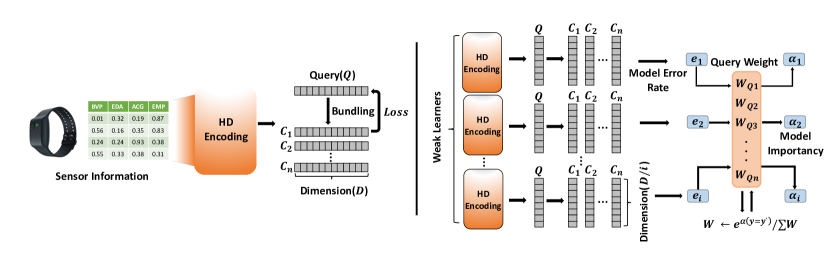
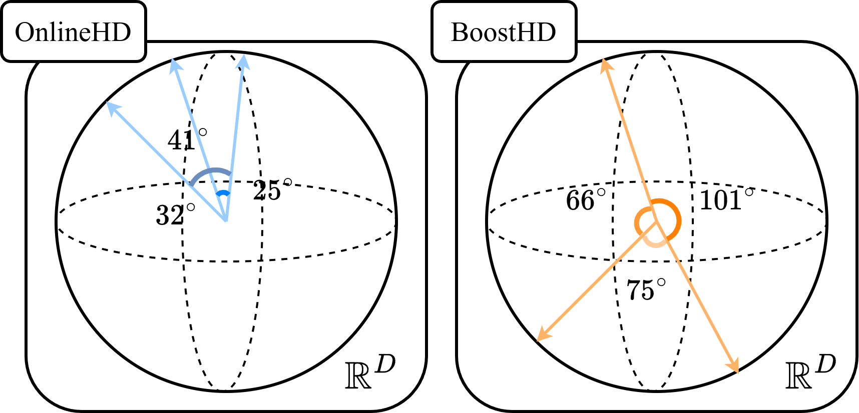
HDC offers promising attributes to effectively address the limitations associated with traditional boosting techniques, as highlighted in prior studies [9, 10]. However, a simplistic parallel ensemble of HDC models may inadvertently escalate the computational costs associated with training and may not guarantee robustness against noise for each weak learner. In our approach, we leverage the OnlineHD model [4] as a foundation, proposing a novel partitioning strategy where the model’s hyperdimensional space () is divided among weak learners, with each receiving a dimensional segment. This segmentation approach prompts us to designate these segmented models as weak learners. Subsequently, we analyze the utilization efficiency of the hyperdimensional space by each weak learner Figure 5 and theoretically demonstrate the inherent limitations posed by high-dimensional spaces Equations 3, 2. Under conditions where the performance of weak learners is assured, BoostHD elevates the capabilities of OnlineHD, ensuring stability, and providing robustness against overfitting and noise.
II Related Work
II-A Boosting methods on Machine Learning
To address the limitations of individual predictive models, researchers have explored various ensemble methods that seek to enhance performance by combining multiple models. One such successful ensemble technique is boosting, which sequentially integrates multiple simple models called weak learners and aggregates their predictions to make final decisions. These weak learners are trained to compensate for each other’s prediction errors and can take various forms, including shallow decision trees or a few layers of multi-layer perceptions. One of the pioneering works in boosting is Adaptive Boosting (AdaBoost) [8]. AdaBoost begins by assigning equal weight values to data points within a training set. It then sequentially trains each weak learner, focusing on identifying misclassified data points and increasing their weights to ensure subsequent weak learners prioritize their correct classification. Each weak learner is assigned a confidence value based on its prediction performance, and the final prediction is determined through a confidence-weighted voting mechanism among the weak learners. Another notable approach is the Gradient Boosting Machine (GBM) [11], which differs from AdaBoost by seeking to minimize the residual error rather than assigning weights to data points. GBM also follows a sequential training process, with each weak learner striving to reduce the residual error left by the previous model through gradient descent. Subsequent boosting algorithms, such as Light GBM [12] and XGBoost [13], adopted this residual error minimization approach due to its demonstrated effectiveness in comparison to the data-point weighting strategy initially employed by AdaBoost.
II-B Healthcare with wearable device
The WESAD dataset[14] stands at the forefront of wearable stress and affect detection, providing a comprehensive collection of physiological and motion data from both wrist- and chest-worn devices in a controlled lab environment with 15 subjects. Distinguishing itself through diverse sensor modalities, WESAD captures data such as blood volume pulse, electrocardiogram, electrodermal activity, electromyogram, respiration, body temperature, and three-axis acceleration. Notably, the dataset introduces a unique dimension by including three affective states—neutral, stress, and amusement, enriching its applicability in studying stress and emotions. The prevalent state-of-the-art solution involves varied convolutional neural network (CNN) architectures[15]. Amidst this landscape, Hyperdimensional Computing (HDC) emerges as a compelling alternative to CNN models. The inherent resource constraints of wearable devices, exemplified by WESAD, align seamlessly with HDC’s capabilities. Offering lightweight and online learning, HDC proves to be a natural fit for the intricacies of the WESAD dataset. Unlike conventional CNNs, HDC excels in managing multimodal data, addressing the varied sensor modalities present in WESAD. The fusion of WESAD’s rich sensor modalities and affective states with the computational robustness of HDC holds great promise for real-world applications in wearable stress and affect detection, presenting WESAD as an ideal testing ground for harnessing the power of hyperdimensional computing.
II-C Hyperdimensional Classification
| (1) |
HDC is a computational technique inspired by the neural processes in the brain, where data points are encoded into a high-dimensional space. The learning process in HDC involves extracting universal patterns that define each label in a dataset through matrix multiplication using Gaussian distribution values and trigonometric activation functions(Binding, Permutation), such as cosine and sine. The encoded hypervectors are linearly combined to generate representations for each class (Bundling), known as class hypervectors . These are represented as single points in the space, and upon end of training, a point is produced for each label in the classification task, as illustrated in Figure 5. During the inference phase of HDC, a query hypervector is encoded, and its similarity to the is calculated. The class whose exhibits the highest similarity to the query is predicted as the output. Recently, the similarity computation between each data point and the using a similarity function has been employed to guide model updates [4]. This is based on assessments of similarity and correctness, facilitating an iterative refinement process. Such a process enhances the HDC model’s ability to capture underlying data patterns, thereby improving its predictive accuracy.
-
•
(1) Bundling consists of an addition of multiple hypervectors into a single hypervector, . This process transforms into memorization in high-dimensional space.
-
•
(2) Binding associates multiple orthogonal hypervectors (e.g., , ) into a single hypervector (). The binded hypervector is a new object in HDC space which is orthogonal to all input hypervectors ( and ).
-
•
(3) Permutation defines as a single rotational shift. The permuted hypervector will be nearly orthogonal to its original hypervector ().
Input:
: Set of data points
: Labels
: Test data point
Parameters:
: Dimensionality
: Number of learners
: Sample weight
Output:
: Trained learners parameterized by
: Weight of learner
: Prediction
III Boosting Hyperdimensional Computing
In this section, we introduce the BoostHD framework, integrating boosting techniques into HDC with a focus on dimensionality (). Instead of relying solely on a single robust learner with high , this approach breaks down the dimension into numerous sub-dimensions, each represented by a weak learner. These weak learners are trained sequentially, with each one adaptively learning from and correcting the errors of its predecessor. This methodology effectively addresses the limitations of the strong learner, thereby enhancing its performance ceiling (as outlined in Algorithm 1). A notable feature of this method is its sequential training process, while parallelization becomes feasible during the inference phase.
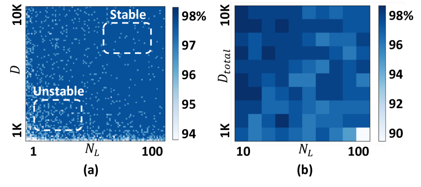
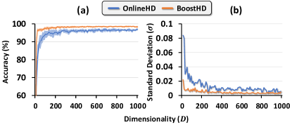
Performance, assessed based on the parameters and the number of weak learners (), shows a direct relationship, ensuring stable and improved performance with substantial values for both and , as depicted in Figure 3. However, it’s crucial to note that elevated values of and introduce increased computational costs, establishing an inherent tradeoff between computational cost and performance. To maintain the effectiveness of weak learners, preserving a baseline dimensionality is imperative.Failure to do so, as exemplified in the case where and , can lead to a substantial degradation in performance, as demonstrated in Figure 3(b).
| (2) |
| (3) | ||||
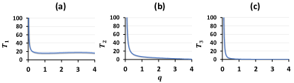
In the context of HDC, partitioning dimensions can be viewed as a transformation in the geometric shape of the kernel (). HDC frameworks often employ the Gaussian Kernel as their foundational element, represented as . When this kernel transforms a hyperdimensional space, the geometric characteristics of can be described by leveraging the theory of the Marchenko-Pastur distribution of random matrices ([16]). Equations 2 and 3 provide insights into this process. Here, is defined as the ratio of the number of columns () to the number of rows (), represents the standard deviation of the Gaussian distribution (i.e., 1), denotes singular values, and and signify the upper and lower bounds of . The mean and variance of are expressed in Equations 2 and 3, respectively. Considering that is determined by the dataset, and is a parameter represented by , under the assumption of a fixed input shape, it becomes evident that exhibits an inverse relationship with , while demonstrates a direct proportionality with . Conversely, Equation 3 formulates as a function of three distinct terms: (Equation 4), (Equation 5), and (Equation 6). Each term converges to a specific value and experiences minimal fluctuations after that. Consequently, increases directly in proportion to , while remains constant as increases.
This proportionality implies that irrespective of the values of and , maintains a consistent absolute interval value due to the stability of (Equation 7). As increases, the values of escalate, yet the interval remains steady. This phenomenon results in the ratio of the minor axis () to the major axis () asymptotically approaching unity (i.e., 1), leading to a circular shape. This observation underscores the pivotal role of in shaping the kernel, wherein an elliptical kernel is transformed into a broadly distributed circular shape beyond the constrained space formed by input biases, as illustrated in Figure 4.
| (4) | |||
| (5) | |||
| (6) | |||
| (7) |
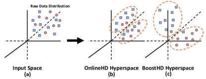
Within the framework of HDC, the theoretical definition of utilizing the subspace formed by classifiers can be expressed as , where represents the rank of the matrix formed by the classifier, and signifies the dimensionality of the space. However, in practical applications, the effective span of the subspace experiences attenuation due to various factors denoted by . These factors are the product sums of cosine similarity values between class hypervectors, which embody constraints or characteristics inherent to the system. Consequently, the actual Span Utilization () is defined as the quotient of divided by the product of . This representation encapsulates the reduced space that is practically attainable, considering the influence of the aforementioned factors. In the realm of HDC, where cosine similarity serves as the metric of choice, maximizing the utilization of this subspace directly impacts the system’s performance. With a focus on optimizing (as depicted in Figure 5), the BoostHD approach is superior to traditional HDC methodologies. By augmenting the subspace’s utilization, BoostHD optimizes computational resources and significantly enhances the accuracy and efficiency of high-dimensional data processing. This observation underscores the practical relevance of subspaces in HDC and highlights the pivotal role played by BoostHD in maximizing their utility.
IV Evaluation
In our experimental setup, we employed a single GPU, the GeForce RTX 4070, and a 12th generation Intel(R) Core(TM) i7-12700K CPU. We conducted a total of 10 runs for each experiment, utilizing datasets that included WESAD[14], the Nurse Stress Dataset[17], and the Stress-Predict Dataset[18] to evaluate accuracy and time efficiency. For all other aspects of the experiments, we exclusively employed the WESAD[14] dataset. The WESAD[14] dataset holds a prominent position as a benchmark dataset tailored for stress detection research. It encompasses multimodal sensor data collected from wearable devices such as Empatica E4 and RespiBAN, sourced from 16 subjects. This dataset encompasses a rich array of physiological and motion data indicators, encompassing EDA, ECG, EMG, and BVP readings. The Stress-Predict Dataset[18] and Nurse Stress Dataset[17] datasets, on the other hand, are solely collected via the E4 sensor and share features like EDA, ECG, EMG, and BVP. Notably, the Nurse Stress Dataset[17] and Stress-Predict Dataset[18] datasets include 37 and 15 subjects, respectively. We performed stress level classification, reducing it to three labels (good, common, stress), and the test data was organized based on subject units, with all results grounded in the test dataset.
Datasets undergo preprocessing using a moving average filter with a window size of 30, extracting statistical measures like minimum, maximum, mean, and standard deviation. Due to the varied ranges of these statistics, normalization is applied to ensure consistent scaling. Our experimental models include AdaBoost with learning rate (lr) set to 1.0 and 10 estimators, Random Forest with bootstrap enabled and 10 estimators, XGBoost with 10 estimators, SVM with a linear kernel, DNN consists of convolutional layers with a learning rate of 0.001, 4 linear layers [2048,1024,512,classes], ReLU activation, and dropout. Additionally, OnlineHD is configured with dimension adjustment, bootstrap enabled, lr of 0.035, and a gaussian probability distribution (0, 1). These setups ensure a comprehensive evaluation of model performance across various algorithms in the experimental framework. In the ensemble models, we employed . The HDC model was configured with values spanning the range . As for the BoostHD model, the weak learner () dimensionality () was set as .
| Dataset | Adaboost | RF | XGBoost | SVM | DNN | OnlineHD | BoostHD |
|---|---|---|---|---|---|---|---|
| WESAD | 93.13 0.01 | 97.13 0.06 | 96.88 0.01 | 93.12 0.01 | 96.75 1.05 | 96.37 0.40 | 98.37 0.32 |
| Nurse Stress Dataset | 55.28 0.01 | 59.35 0.78 | 61.01 0.01 | 60.99 0.01 | 60.04 0.06 | 61.37 0.10 | 61.52 0.07 |
| Stress-Predict Dataset | 67.54 0.01 | 67.76 0.12 | 65.76 0.01 | 67.30 0.01 | 67.29 0.07 | 65.79 0.17 | 68.10 0.09 |
| Dataset | Adaboost | RF | XGBoost | SVM | DNN | OnlineHD | BoostHD |
|---|---|---|---|---|---|---|---|
| WESAD | 46.3 | 38.5 | 47.6 | 108.3 | 37.0 | 7.57 | 11.0 |
| Nurse Stress Dataset | 145.2 | 179.7 | 131.1 | 188.4 | 38.6 | 14.5 | 12.1 |
| Stress-Predict Dataset | 63.4 | 91.5 | 58.7 | 265 | 43.7 | 13.2 | 12.0 |
IV-A Performance
In our comprehensive experimentation, we subjected the BoostHD algorithm to rigorous evaluation across three distinct datasets: WESAD[14], Nurse Stress Dataset[17], and Stress-Predict Dataset[18]. The focal points of our assessment encompassed key metrics such as accuracy, inference time, and training time. Our findings unveiled the remarkable prowess of BoostHD, consistently attaining the highest accuracy levels across all three datasets, as presented in Table I. Notably, when compared to OnlineHD on the WESAD[14] dataset, the accuracy achieved by BoostHD remained outside the range of two standard deviations. This distinction was further underscored by OnlineHD’s inability to reach a 98% accuracy threshold in any of the ten independent trials, while BoostHD consistently surpassed this benchmark, highlighting its superior predictive accuracy.
BoostHD strategically harnesses in-memory learning, epitomized by HDC, and augments it with adaptive learning mechanisms within an ensemble framework. This unique fusion results in a significant acceleration of the learning process, even when training is serialized. Empirical assessments conducted within a GPU environment unequivocally established BoostHD’s superiority over DNNs, demonstrating substantially enhanced processing speed across the three benchmark datasets. Moreover, in a CPU environment, BoostHD showcased remarkable computational efficiency, achieving processing speeds 26 times faster than its DNN counterparts. Furthermore, our optimization efforts fine-tuned the BoostHD algorithm for parallel processing, yielding substantial gains in inference efficiency (as detailed in Table II). This optimization proved particularly beneficial when handling the relatively extensive input vectors in the Nurse Stress Dataset[17] and Stress-Predict Dataset[18]. The outcome was a significant reduction in the time required for inferring data from the test dataset, firmly establishing BoostHD as the model of choice for maximizing time efficiency across all models evaluated, especially in the context of the Nurse Stress Dataset[17] and Stress-Predict Dataset[18].
IV-B Stability
BoostHD demonstrates strong and consistent performance and exhibits stable convergence even in constrained environments. As illustrated in Figure 3, the accuracy of the weak learner experiences a steep decline when the minimum dimensionality requirement is unmet. By ensuring this minimum dimensionality and progressively increasing the value of , we observe a clear separation between the two models within a given one standard deviation (), as shown in Figure 6(a). Specifically, the value of for BoostHD stands at 0.0046, while for OnlineHD, it registers at 0.0127, signifying a roughly threefold disparity. This lower value for BoostHD underscores its superior stability. In the context of BoostHD, it’s notable that scales proportionally with and inversely with provided that the baseline condition is maintained (as depicted in Figure 3(a), upper right). Moreover, when the value of surpasses a specific threshold (), such as 50 as illustrated in Figure 3(a) (i.e., ), the value remains consistently preserved.
| Left hands | Female | Age 25 | Age 30 | Height 170 | Height 185 | AVERAGE | |
|---|---|---|---|---|---|---|---|
| Adaboost | 95.63 | 96.86 | 96.05 | 89.24 | 90.74 | 91.27 | 93.30 |
| RF | 97.15 | 97.7 | 98.03 | 88.29 | 95.06 | 94.92 | 95.19 |
| XGBoost | 98.73 | 98.12 | 98.68 | 91.41 | 95.06 | 94.24 | 96.04 |
| SVM | 97.47 | 95.4 | 94.74 | 92.41 | 90.12 | 95.24 | 94.23 |
| DNN | 98.42 | 95.4 | 94.41 | 88.92 | 92.59 | 93.57 | 93.89 |
| OnlineHD | 98.73 | 97.8 | 94.08 | 92.41 | 92.59 | 94.6 | 95.04 |
| BoostHD | 99.05 | 98.33 | 96.38 | 93.35 | 96.3 | 93.73 | 96.19 |
IV-C Overfitting
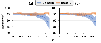
BoostHD presents a noteworthy advantage over traditional HDC methods in its resilience to overfitting. To empirically assess this characteristic, we intentionally induce overfitting by crafting an imbalanced dataset () through the generation of data subsets. The extent of overfitting, denoted as , is quantified by creating subset data for all classes except the target class (). This process yields the final dataset as described in Equation 8. We employ Macro accuracy as a more suitable metric for imbalanced datasets to ensure a fair performance evaluation that the varying sample counts per class do not skew. As the value of increases, OnlineHD experiences a noticeable decline in performance. In stark contrast, BoostHD consistently maintains its performance levels, demonstrating a robust ability to preserve stability, as depicted in Figure 7.
| (8) |
IV-D Robustness
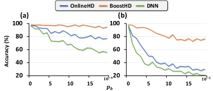
We assess the robustness of models against bitflip noise to explore in wearable device originating from hardware components according to its probability of bit flip error . In Figure 8, our experiments spanned two distinct ranges of , given the substantial impact of this parameter on performance. Our experimental scope was deliberately limited to a narrow range of . Despite this inherent constraint and our meticulous approach of conducting 100 independent trials to ensure statistical validity, we observed occasional peaks in the graph. Nevertheless, a discernible trend as a function of persisted. Within the range where , as illustrated in Figure 8(a), BoostHD incurred an accuracy loss of no more than 5.7%. This represents approximately one-fourth of the loss observed in OnlineHD and roughly one-seventh of that observed in DNN. To statistically validate the accuracies concerning varying , we employed the Median Absolute Deviation (MAD) as a measure of robustness (defined as ). In Figure 8(a), the MAD for BoostHD was quantified at 0.024, which is six times lower than that of OnlineHD (0.1454) and four times lower than that of DNN (0.083). In Figure 8(b), BoostHD exhibited a MAD of 0.005, which is three times lower than OnlineHD (0.015) and a substantial 30 times lower than DNN (0.1509). These results are compelling evidence of BoostHD’s superior robustness compared to the other methods.
IV-E Bias and reliability for person-specific groups
We carefully segmented subjects based on various attributes in WESAD[14], including hand preference, gender, age, and height. This stratification resulted in subsets with specific subject characteristics, such as left-hand preference, female gender, age groups, and height categories. Our primary objective was to assess how well models performed across individuals with diverse characteristics, a crucial consideration for healthcare applications to ensure fairness and accuracy. Notably, our BoostHD model consistently outperformed other models in all categories III, except for two cases where it ranked second. This underscores the potential of combining boosting methods and HDC, especially in healthcare, where equitable performance is essential.
V Conclusion
We introduced BoostHD, a novel method that integrates hyperdimensional computing with boosting to create a robust ensemble model. BoostHD effectively overcomes limitations of traditional HDC by efficiently utilizing high-dimensional spaces and preventing overfitting. Our experiments on healthcare datasets demonstrated that BoostHD consistently outperforms existing methods in accuracy, efficiency, stability, and robustness. These results confirm BoostHD’s potential in critical domains where reliability and precision are essential.
Acknowledgements
This work was supported in part by the DARPA Young Faculty Award, the National Science Foundation (NSF) under Grants #2127780, #2319198, #2321840, #2312517, and #2235472, the Semiconductor Research Corporation (SRC), the Office of Naval Research through the Young Investigator Program Award, and Grants #N00014-21-1-2225 and #N00014-22-1-2067, Army Research Office Grant #W911NF2410360. Additionally, support was provided by the Air Force Office of Scientific Research under Award #FA9550-22-1-0253, along with generous gifts from Xilinx and Cisco.
References
- [1] D. Kleyko, D. Rachkovskij, E. Osipov, and A. Rahimi, “A survey on hyperdimensional computing aka vector symbolic architectures, part ii: Applications, cognitive models, and challenges,” ACM Computing Surveys, vol. 55, no. 9, pp. 1–52, 2023.
- [2] S. Yun, H. E. Barkam, P. R. Genssler, H. Latapie, H. Amrouch, and M. Imani, “Hyperdimensional computing for robust and efficient unsupervised learning,” in 2023 57th Asilomar Conference on Signals, Systems, and Computers. IEEE, 2023, pp. 281–288.
- [3] S. Yun, R. Masukawa, S. Jeong, and M. Imani, “Spatial-aware image retrieval: A hyperdimensional computing approach for efficient similarity hashing,” arXiv preprint arXiv:2404.11025, 2024.
- [4] A. Hernandez-Cane et al., “Onlinehd: Robust, efficient, and single-pass online learning using hyperdimensional system,” in DATE, 2021.
- [5] X. Ying, “An overview of overfitting and its solutions,” in Journal of physics: Conference series, vol. 1168. IOP Publishing, 2019, p. 022022.
- [6] C. Rudin, “Stop explaining black box machine learning models for high stakes decisions and use interpretable models instead,” Nature machine intelligence, vol. 1, no. 5, pp. 206–215, 2019.
- [7] Y. Kumar, A. Koul, R. Singla, and M. F. Ijaz, “Artificial intelligence in disease diagnosis: a systematic literature review, synthesizing framework and future research agenda,” Journal of ambient intelligence and humanized computing, pp. 1–28, 2022.
- [8] R. E. Schapire, “Explaining adaboost,” in Empirical Inference: Festschrift in Honor of Vladimir N. Vapnik. Springer, 2013, pp. 37–52.
- [9] D. Kleyko, D. Rachkovskij, E. Osipov, and A. Rahimi, “A survey on hyperdimensional computing aka vector symbolic architectures, part ii: Applications, cognitive models, and challenges,” ACM Computing Surveys, vol. 55, no. 9, pp. 1–52, 2023.
- [10] A. Thomas, S. Dasgupta, and T. Rosing, “A theoretical perspective on hyperdimensional computing,” Journal of Artificial Intelligence Research, vol. 72, pp. 215–249, oct 2021. [Online]. Available: https://doi.org/10.1613%2Fjair.1.12664
- [11] J. H. Friedman, “Greedy function approximation: a gradient boosting machine,” Annals of statistics, pp. 1189–1232, 2001.
- [12] G. Ke, Q. Meng, T. Finley, T. Wang, W. Chen, W. Ma, Q. Ye, and T.-Y. Liu, “Lightgbm: A highly efficient gradient boosting decision tree,” Advances in neural information processing systems, vol. 30, 2017.
- [13] T. Chen, T. He, M. Benesty, V. Khotilovich, Y. Tang, H. Cho, K. Chen, R. Mitchell, I. Cano, T. Zhou et al., “Xgboost: extreme gradient boosting,” R package version 0.4-2, vol. 1, no. 4, pp. 1–4, 2015.
- [14] P. Schmidt, A. Reiss, R. Duerichen, C. Marberger, and K. Van Laerhoven, “Introducing wesad, a multimodal dataset for wearable stress and affect detection,” in Proceedings of the 20th ACM international conference on multimodal interaction, 2018, pp. 400–408.
- [15] A. Reiss, I. Indlekofer, P. Schmidt, and K. Van Laerhoven, “Deep PPG: Large-Scale heart rate estimation with convolutional neural networks,” Sensors (Basel), vol. 19, no. 14, Jul. 2019.
- [16] F. Götze and A. Tikhomirov, “Rate of convergence in probability to the marchenko-pastur law,” Bernoulli, vol. 10, no. 3, pp. 503–548, 2004.
- [17] S. Hosseini, R. Gottumukkala, S. Katragadda, R. T. Bhupatiraju, Z. Ashkar, C. W. Borst, and K. Cochran, “A multimodal sensor dataset for continuous stress detection of nurses in a hospital,” Scientific Data, vol. 9, no. 1, p. 255, 2022.
- [18] T. Iqbal, A. J. Simpkin, D. Roshan, N. Glynn, J. Killilea, J. Walsh, G. Molloy, S. Ganly, H. Ryman, E. Coen et al., “Stress monitoring using wearable sensors: A pilot study and stress-predict dataset,” Sensors, vol. 22, no. 21, p. 8135, 2022.