Population dynamics of multiple ecDNA types
Abstract
Extrachromosomal DNA (ecDNA) can drive oncogene amplification, gene expression and intratumor heterogeneity, representing a major force in cancer initiation and progression. The phenomenon becomes even more intricate as distinct types of ecDNA present within a single cancer cell. While exciting as a new and significant observation across various cancer types, there is a lack of a general framework capturing the dynamics of multiple ecDNA types theoretically. Here, we present novel mathematical models investigating the proliferation and expansion of multiple ecDNA types in a growing cell population. By switching on and off a single parameter, we model different scenarios including ecDNA species with different oncogenes, genotypes with same oncogenes but different point mutations and phenotypes with identical genetic compositions but different functions. We analyse the fraction of ecDNA-positive and free cells as well as how the mean and variance of the copy number of cells carrying one or more ecDNA types change over time. Our results showed that switching does not play a role in the fraction and copy number distribution of total ecDNA-positive cells, if selection is identical among different ecDNA types. In addition, while cells with multiple ecDNA cannot be maintained in the scenario of ecDNA species without extra fitness advantages, they can persist and even dominate the ecDNA-positive population if switching is possible.
Introduction
Cancer is the uncontrolled growth of abnormal cells, and it develops from a single cell to bigger masses which take control of portions of healthy tissues [31, 26]. Following the Darwinian evolution theory, in order to successfully invade, tumour cells obtaining simple or complex variations can survive and escape the normal control mechanism of tissues [2, 25, 3]. One efficient way is through copy number alteration, including amplification of functional genomics sequences such as oncogenes [31, 4]. The amplification of specific oncogenes can happen through extra chromosomal DNA (ecDNA) and homogeneously staining regions (HSRs), which are thought to be the cytogenetic hallmarks of gene amplification in cancers [16]. There is much research related to HSRs [16, 1], but the role of ecDNA in driving tumor expansion and treatment resistance has been largely underestimated for many years. Recently, many studies suggested that patients with tumours containing ecDNA have worse clinical outcomes [14, 11]. "Hiding" oncogenes within ecDNA fragments is a strategic mechanism for the evolution of cancer cells, as this relocation effectively liberates these elements from the normal chromosomal constraints like centromeres, consequently giving tumors the ability to undergo accelerated evolution compared to chromosomal genomes.
The observed ecDNAs are relatively large (1.3 Mb on average) and highly amplified circular structures containing genes and regulatory regions [31], and they make unique contributions to oncogenic transcription and tumour progression through their promotion of oncogene amplification and treatment resistance [11, 27, 24, 30, 20, 6]. The origin of ecDNA has been long studied, and several possible mechanisms have been proposed, including the breakage-fusion-bridge (BFB) cycle, translocation-deletion-amplification model, “episome” model and chromothripsis [32, 28]. The segregation patterns of ecDNA elements in cell divisions have been investigated throughfully, with the common conclusion that unlike DNA, ecDNA copies are randomly partitioned to the daughter cells from the mother [11, 23, 15, 10], and this fuels a fast accumulation of intercellular copy number heterogeneity. A basic mathematical model of tumour dynamics with a single ecDNA type has already been developed [15], where the random segregation and driver role of ecDNA elements in tumour expansion has been validated through an integration of theory and experimental and clinical data [15]. Here, we move beyond the single ecDNA type hypothesis and investigate the population dynamics of multiple ecDNA types.
There are multiple reasons and evidence why we need a general mathematical framework to model multiple ecDNA types, which can refer to ecDNA species carrying distinct oncogenes, genotypes with the same oncogenes but different point mutations, and
phenotypes with identical genetic compositions but different functions generated by phenotypical switching.
First, multiple ecDNAs species originally derived from different chromosomal loci have been observed in the same cancer cell [17, 21]. These ecDNAs can congregate in micron-sized hubs in the nucleus [20, 22] and enable intermolecular gene activation, where enhancer elements on one ecDNA molecule can activate coding sequences on another ecDNA [21]. Second, ecDNAs own clustered somatic mutations [5, 12] which change the genotype of ecDNA and may alter the function of ecDNA sequences with potential phenotypic evolution like in resistance. Third, ecDNA is particularly sensitive to different epigenetic states, which have been associated with responses to site of growth [13, 18] and to stress, including hypoxia and high acidity encountered in tumour microenvironments [15, 17], and activation or deactivation of different oncogenes. This means even without any genetic alternations, ecDNA might switch between different phenotypical states intrinsically.
Considering that experimental evidence shows the most prevalent presence of two ecDNA species in human cancer cells [21], we focus on our analysis of an evolutionary process with two ecDNA types. However, we can extend our general framework to model any number of ecDNA types. Specifically, we model the segregation, possible switching and selection of two ecDNA types in a growing population. Our investigation demonstrates that the stochastic segregation of extrachromosomal DNA yields diverse outcomes under selection and different switching scenarios. While selection significantly impacts the population composition of ecDNA-positive and ecDNA-free cells, as well as the mean, variance, and distribution of ecDNA copy numbers in the total population, switching only plays a role in these quantities when selection differs between the cells carrying different ecDNA types. However, if we classify the cell population into different subgroups based on composition of ecDNA types within a cell, we observe distinct dynamics of cells carrying different types of ecDNA by varying switching strengths. This holds even when selection is identical for different ecDNA types.
More specifically, we examined genotypes with extremely low switching rates or phenotypes with relatively higher switching rates, the mean copy number and proportion of cells in subgroups are significantly influenced by the switching rate.
Methods
A general framework of two ecDNA types
We consider two types of ecDNA, denoted as yellow and red respectively in Figure 1. The reproduction rates (fitness in our model) of the two ecDNA types are and , which are equal to if the selection between ecDNA-positive or ecDNA-free cells is neutral. This means that cells carrying ecDNA have the same fitness as cells without ecDNA under neutral selection, which is normalised to . Alternatively, cells carrying ecDNA types can have fitness advantages compared to ecDNA-free cells, including two scenarios depending on whether the reproduction rates of carrying different ecDNA types equal () or not (). For the sake of simplicity, we assume a cell carrying a mix of yellow and red ecDNA elements has a reproduction rate as the maximum value between and (Figure 1d). This refers to an assumption that having both ecDNA types does not lead to an extra fitness advantage, which does not change our general framework and equations and can be easily released for an extension of analysis [21].
During each cell division, the ecDNA copies are duplicated similar to the chromosomal genetic materials, but due to lack of centromeres the two types of ecDNA copies are randomly partitioned into the two daughter cells independently following a separate binomial distribution with the probability of a single copy segregated to any daughter cell as . Note we can also release the assumption of the independent segregation between the two ecDNA species with evidence-based motivations [21]. For our general framework, we focus on the analysis with independent segregation.
We introduce two probabilities and in the range , representing switching between ecDNA types coupled with cell divisions. If , switching is off and the two ecDNA types refer to different ecDNA species (Figure 1b), where e.g. distinct oncogenes or enhancers are carried in the ecDNA elements and thus there is no one-step transition between the two ecDNA types. If at least one of and is greater than 0, then we consider the propagation of two ecDNA genotypes or phenotypes (Figure 1a). Small values of and can refer to a genotypic change through e.g. point genetic mutations. With an ecDNA sequence size of Mb and a mutation rate of to per base pair, or could be in the order of to . Larger values of and (but still far less than ) can be interpreted as intrinsic phenotype switching, where epigenetic changes such as through DNA methylation [11, 19] or other molecular events alter the ecDNA phenotypes.
In a growing population, the random segregation and/or possible switching between the two ecDNA types promote a high heterogeneity among cells, which can be classified into four different subpopulations, i.e. pure yellow, pure red, mix and ecDNA-free cells (Figure 1cd). We are interested in how the interplay between all evolutionary parameters will impact the dynamics of different subpopulations.

| probability of switching from yellow to red ecDNA | |
| probability of switching from red to yellow ecDNA | |
| reproduction rate for cells carrying only yellow ecDNA | |
| reproduction rate for cells carrying only red ecDNA | |
| proportion of cells carrying at least one ecDNA copy | |
| proportion of cells carrying no ecDNA copies | |
| loss rate of ecDNA due to a completely asymmetric segregation | |
| number of cells carrying yellow and red ecDNA copies at time | |
| frequency of cells carrying yellow and red ecDNA copies at time | |
| loss/gaining rates for ecDNA evolutionary process | |
| population growth factor at time | |
| number of cells carrying ecDNA copies at time | |
| zeroing function for ecDNA-free cells trend | |
| normalising function for ecDNA-free cells trend | |
| -order moment for the whole population at time | |
| -order moment for pure yellow ecDNA cells at time | |
| -order moment for pure red ecDNA cells at time | |
| -order moment for mix ecDNA cells at time |
Deterministic dynamics
These interactions can be expressed by two different mathematical approaches, which are a deterministic one comprising a system of ordinary differential equations (ODEs) and a demographic one comprising a system of stochastic equations. Starting from the system of ODEs, we analyse the densities of cells with and without ecDNA copies denoted by and respectively with,
| (1) |
The above system is justified by observing that cells carrying ecDNA can lose all ecDNA copies, but the reverse is not possible. Because the origin of ecDNA is often considered a random event due to genomics instability, and generally a specific ecDNA can not be gained back once lost in a population. Moreover, the function corresponds to the at the moment undetermined loss rate of ecDNA due to complete asymmetric segregation, i.e. a daughter cell inherited all copies and the other one none by chance. In the case of two ecDNA types, we can split the density function into the sum of three subfunctions: , and , respectively for pure yellow, pure red and mix cells:
| (2) |
We can recover Eqs. (1) by summing the three equations in Eqs. (2) and generalise Eqs. (2) to positive selection cases by multiplying each subpopulation by its own selection coefficient, , or .
Master equation
The ecDNA content of daughter cells at each division depends on the outcome of the random segregation and the switching probability. We can write the probability for a daughter to carry yellow ecDNA copies, given a mother with yellow copies and red copies as
and the one for a daughter to carry red copies, given the same mother as
Based on these preliminary observations, we can then write down the demographic equations as below:
| (3) | ||||
where indicates the number of cells with yellow and red copies at time . Without loss of generality, we can set , then the fitness advantage for mix cells is the maximum between and , thus (Figure 1d).
Results
We are interested in the dynamics of pure, mix and ecDNA-free cells. Thus, we investigate how selection strength and switching parameters lead to different patterns. Again in the results, refers to multiple ecDNA species, otherwise it refers to multiple ecDNA genotypes or phenotypes. indicates neutral selection, indicates identical positive selection, and is for non-identical positive selection.
Copy number distribution of all ecDNA-positive cells and fraction of ecDNA-free cells over time
Let us first look at the scenarios where both yellow and red ecDNAs have the same reproduction rate, i.e. , where . From Eqs. 3, setting as stated, we can recover the dynamics of the number of cells with ecDNA copies at time , as
| (4) | ||||
and we can write
| (5) | ||||
Using the definition of cell frequency (see Table 1):
| (6) |
together with Eqs. (4) and (5), we can find that the total population size, under different selection scenarios as
| for , | (7) | ||||
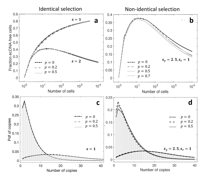
Eqs. (5) and (7) show that, when the selection strength is identical for cells carrying any of the two ecDNA types, the distribution of total ecDNA copies remains to be independent of the switching rates over time (Figure 2c).
This independence from switching probabilities holds for the fraction of ecDNA-free cells over time as well (Figure 2a). Indeed, using Eqs. (1) based on our methods of modeling single ecDNA types in [15], we can obtain solutions for and get the frequency of ecDNA-free cells as
| (8) | ||||
| and | ||||
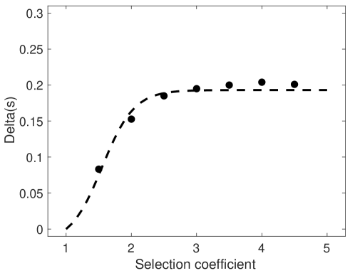
Whilst the fraction of ecDNA-free cells, , is approaching 1 as for neutral selection (), we expect the progressive decrease of the fraction of cells carrying ecDNA. On the contrary, shrinks to zero under identical positive selection (). We can measure how fast this trend is approaching by approximating the function at the denominator of the second equation in Eqs. (8), which is modulated by . Using Monte Carlo simulations and studying the shape of the fitting curve, we approximate
| (9) |
As is almost stable for , solution in (9) suggests the existence of a fitness threshold, after which the zeroing of is not affected by further increasing (Figure S1).
Now we look at the scenario where fitness for cells carrying different ecDNAs is not identical (). The copy number distribution of total ecDNA-positive cells and the fraction of ecDNA-free cells are highly sensitive to selection coefficients ( Figure 2b&d). The independence of those quantities on the switching rates, and , is lost.
To understand the cell dynamics and population composition of different ecDNA types, we look at subgroups of ecDNA-positive cells instead of the total number, and separate our moment analysis when type switching is off (ecDNA species) or on (ecDNA genotypes or phenotypes).
Moment analysis for multiple ecDNA species when switching is off
We can study the dynamics of two ecDNA species by plugging in Eqs. (3), obtaining the following demographic system as
| (10) | ||||
Using Eqs. (7) and (3), we calculate the -order moment for each subpopulation by the formula
| (11) |
where is respectively for pure yellow, pure red and mix subpopulations.
We focus on the case of identical fitness, i.e. including scenarios under neutral selection and positive selection . Starting with , we write exact equations for probability densities of pure and mix cells over time using Eqs. (6). For example, for pure yellow cells, we have
| (12) |
Then, Eq. (12) can be substituted in Eq. (11) to get every -order moment. The first moment dynamic, which describes the average copy number of pure cells carrying only yellow ecDNA copies, is given by
|
|
(13) |
Similarly. we can obtain the first moment dynamics for pure red and mix subpopulations (see Table 2).
Now we move to the scenario of identical positive fitness, i.e , combining Eqs. (5) and (7), we obtain the frequencies of pure yellow ecDNA cells as
| (14) |
Using the moment calculation formula in (11) we get
| (15) |
The same steps in (12) and (15), together with standard solution techniques for ODEs, are used for filling Table 2. The total moment has been already given [15]:
| (16) | |||||
| and | |||||
| Weighted first moment dynamics equations for ecDNA species | |||
|---|---|---|---|
| Neutral case | |||
| Subpopulation | Equation | Solution | |
| Total | |||
| Pure yellow | |||
| Pure red | |||
| Mix | |||
| Identical positive selection case | |||
| Subpopulation | Equation | Solution | |
| Total | |||
| Pure yellow | |||
| Pure red | |||
| Mix | |||
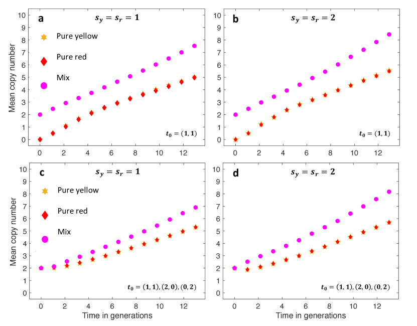
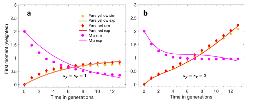
Our analytical results, where the integral on the ecDNA-free cells density has been calculated numerically and the constant of integration has been inferred by using Monte Carlo methods, match well with stochastic simulations implemented by Gillespie Algorithm [29, 7, 8, 9] (Figure 3).
Our moment analysis of each sub-populations refers to weighted moments, which consider the variability in copy numbers across different subpopulations together with their respective fractions relative to the total population size. Specifically, the weighted mean copy number shown are normalised based on the mean copy number for the total population. For example, the mean copy number for the total population used for the normalisation is constant under neutral selection, which is as the copy number of the initial cell in Figure 3a. Under identical positive selection, it is in Figure 3b.
The dynamics of weighted moments align with the trends observed in the unweighted mean copy number dynamics of each subpopulation, as illustrated in Figure S3. In the Supplementary section, we examine every sub-populations separately and track their absolute mean copy numbers over time. As expected, the absolute average copy numbers increase over time for ecDNA-positive cells no matter whether they are pure or mix cells. However, the changes in curve slopes portrayed by the weighted moments in Figure 3 suggest that, despite the steady increase in the absolute number of ecDNA copies in both pure and mix cells, the proportion of pure cells contributes more substantially than mix ones to the mean copy number of the total population if selection is identical (neutral and positive).
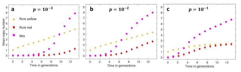
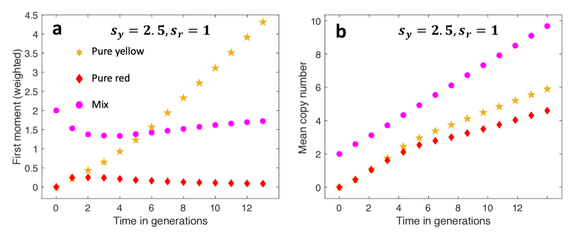
While it is difficult to obtain analytical solutions for the non-identical selection case, we simulate the weighted first moment (Figure S6a) and absolute mean copy number (Figure S6b) for the case of two ecDNA species, where the cells carrying yellow ecDNA are assumed to proliferate faster than the cells carrying red ecDNA. Conversely to the dynamics under identical positive selection (Figure 3b and Figure S3b&d), pure yellow ecDNA cells dominate the populations over time as expected (Figure S6a). However, since we assume that mix cells have the same fitness as the fitter pure cells, the contribution of mix cells to the whole population is much less than the one of pure cells, no matter if under identical positive selection or non-identical selection. In the infinite time limit, the mix cells cannot be maintained.
Moment analysis of multiple ecDNA genotypes or phenotypes when switching is on
Under identical fitness and one-way switching
Now we analyse the dynamics of two ecDNA genotypes or phenotypes, where different types of ecDNA elements can switch to each other. We first look at a simpler case of one-way switching. Without the loss of generality, we can set and . We consider values for which , whose are more biologically relevant. Using the Taylor approximation, we can write
| (17) |
We use the notation L-B and U-B to indicate the lower-bound and upper-bound approximations in (17).
In the simplest case of neutral selection, i.e. , we write exact equations for frequencies of pure, mix and ecDNA-free cells over time using Eqs. (6). For the pure yellow subpopulation, we have
| (18) |
Then, we can substitute Eq. (18) in (11) to get every -order moment. The first moment dynamics, i.e. the average copy number of cells carrying only yellow ecDNA elements, using the L-B approximation, i.e. , , is
| (19) | ||||
Instead, using the U-B approximation, i.e. , , we have
| (20) |
The second moment dynamics measures the variance in copy number, which is obtained under the L-B approximation as
and under the U-B approximation as
The same steps are used for filling Table 3, together with the results for the total moments in Eqs. (16).
| Weighted moment dynamics equations for and | |||
|---|---|---|---|
| First moment dynamics | |||
| Subpopulation | Equation L-B | Equation U-B | |
| Total | |||
| Pure yellow | |||
| Pure red | |||
| Mix | |||
| Second moment dynamics | |||
| Subpopulation | Equation L-B | Equation U-B | |
| Total | |||
| Pure yellow | |||
| Pure red | |||
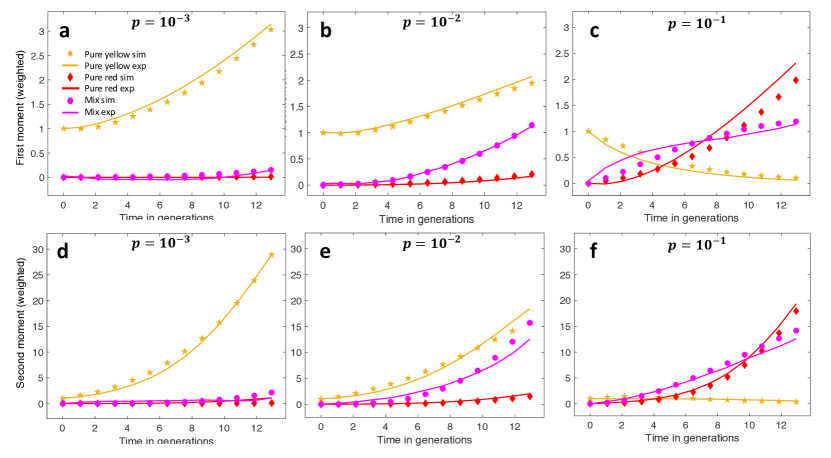
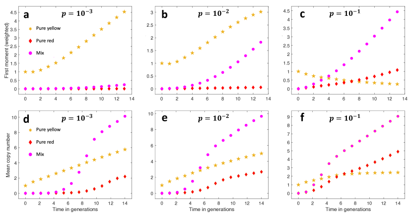
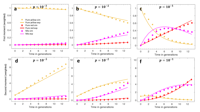
However, the lower-bound equations in Table 3 for neutral selection (and also the ones in Supplementary Table S1 for identical positive selection) do not account for the contribution of pure red cells in the first moment dynamics. When is approximated by zero for small values, it effectively nullifies the contribution of the pure red ecDNA subpopulation in the system, resulting in in this case. This limitation is not present in the upper-bound approximation, where approximates when is sufficiently small, ensuring that the velocity function in the ordinary differential equation for remains positive. Consequently, we focus our analysis on the upper-bound approximation throughout the following sections. Our analytical approximations match well with stochastic simulations (Figure 4 and Figure S2), where it is further noticeable how the upper-bound approximation fits better the stochastic simulations.
Starting from a single cell with one yellow ecDNA copy and one-way switching from yellow to red (), we examine the impact of switching on the weighted mean and variance of the copy number. When the switching rate increases, we observe a decrease of the contribution of pure yellow cells and an increase of the contribution of pure red cells to the ecDNA-positive population, no matter if under neutral selection (Figure 4a-c) or identical positive selection (Figure S2a-c). With increasing switching rates, mix cells can be maintained in the population even without fitness advantages compared to pure cells. However, under neutral selection, ecDNA-positive cells will slowly decrease over time due to random segregation and the accumulation of ecDNA-free cells, thus the impact of switching is stronger in this case compared to the identical positive selection scenario. When analysing small switching rates, we can appreciate indeed a difference between the two selection scenarios. Under neutral selection, the contribution of pure yellow cells decreases over time for small switching values (Figure 4a&b). On the contrary, under positive and identical selection, the ecDNA-positive cells will expand, thus, starting from a pure yellow cell, the contribution of the pure yellow subpopulation still dominates and increases when small values are considered (Figure S2a&b).
The mean copy number aligns well with the weighted first moment dynamics. When selection is neutral, the absolute mean copy number sharply increases for mix cells (Figure S4), and we also observe a rising trend for this subpopulation in the weighted first moment (Figure 4 a-c), measuring the contribution of each subpopulation to the absolute mean copy number of the population. This indicates an increase in the number of mix cells over time among the total population. On the contrary, while pure yellow ecDNA cells exhibit a constant increase in their absolute mean copy number, their decreasing trend in the weighted first moment, inversely proportional to values, suggests a decline in the number of individuals in this subpopulation over time, attributable to the one-way switching discussed above.
Examining the variance (Figure 4 d-f and Figure S2 d-f), we observe similar dynamics to those seen in the first moment, indicating that the weighted variance in mean copy number is higher when the subpopulation is larger. This might be explained by the broad range of copy number configurations expected in a large population due to the nature of cell division.
While obtaining solutions for non-identical selection is difficult, we examine the moment dynamics for this case through stochastic simulations. Again, pure yellow cells are assumed to be fitter than the pure red cells and the switching is one-way, from yellow to red (). Starting from a single pure yellow cell, the dynamics under small switching rates (Figure S7a&b) are very similar to those under identical positive selection (Figure S2a&b), where the contribution of pure yellow cells to the ecDNA-positive population dominates and increases over long time. However, the contribution of the pure red cells remains trivial under non-identical selection scenario (Figure S7b), as they reproduce slower than pure yellow and mix cells. This differs from the identical positive selection case (Figure S2 b). When the switching rate increases, the contribution of the pure yellow cells again decreases (Figure S7c), which holds for all selection scenarios including neutral, identical positive and non-identical selection. However, under higher switching rates, not only the mix cells can be maintained but also dominate the ecDNA-positive population. This phenomenon has been observed only under non-identical selection.
Under identical fitness and two-way switching
Now we investigate the case when both ecDNA types can switch into each other, i.e. . Considering the approximations in (17) and the method in (13), we fill the Table 4.
| Weighted first moment dynamics equations for and | ||
|---|---|---|
| First moment dynamics | ||
| Subpopulation | Equation U-B | |
| Total | ||
| Pure yellow | ||
| Pure red | ||
| Mix | ||
We observe an inner symmetry in the equations in Table (4) in terms of the parameters and . This, we consider an identical switching probabilities scenario for the ecDNA types, i.e. . Focusing on U-B approximation results from Table 4, we aim to solve the following system in matrix form:
| (21) |
The eigenvalues of are , and , with eigenvectors , and . The solutions of (21) are given by
where is the diagonal similar matrix to , is given by and is the vector of initial values , hence:
and by matrix multiplication we get the solutions in Table 5 in case of neutral selection for the whole population.
| Wighted first moment dynamics’ U-B approximation for and | |
|---|---|
| Subpopulation | First moment |
| Total | |
| Pure yellow | |
| Pure red | |
| Mix | by subtraction |

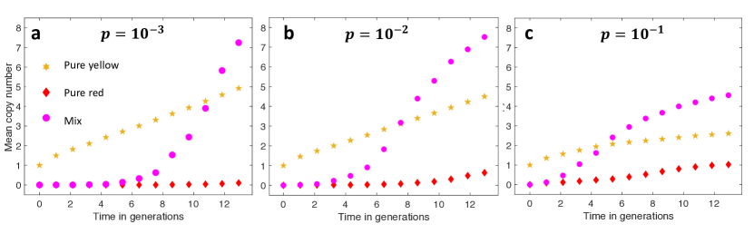
In Figure 5, starting from a single cell with one yellow ecDNA copy and a two-way switching from yellow to red copies and back, we observe a consistent alignment between our analytical approximations and stochastic simulations under neutral selection. Comparing the weighted first moment dynamics with the mean copy number in Figure S4, we observe a more pronounced increase in mix cell trends for both absolute and relative counts when is relatively higher. Conversely, the absolute mean copy number appears to reach a sort of steady state after several generations for pure subpopulations, suggesting that mix cells rapidly become the ones with the highest number of copies in the two-way switching scenario.
Furthermore, by examining the weighted mean copy number in Figure 5, we can draw additional conclusions about the proportion of subpopulations over time. Pure yellow cells decrease in number over time, while mix cells significantly increase. Summarising the results from both absolute and weighted first moments, it appears that mix cells are increasingly dominating the ecDNA-positive cells, carrying also the configurations with the highest copy numbers.
Comparing these observations with the ones under one-way switching, it seems that two-way switching leads to a sharper increase in weighted mean copy number of mix. This suggests the two-way switching promotes the expansion and mantenance of multiple ecDNA types presenting in the same cells.
Discussion
We present a framework to model two ecDNA types, which can be adapted to either species, genotypes or phenotypes, by easily changing the switching probabilities between the two types. If the type switching probability is set to zero for both yellow and red ecDNA, we consider two distinct species; conversely, two genotypes distinct by point mutations with relatively low switching probabilities or phenotypes by phenotypical switching. Similar to previous models on a single ecDNA type [15, 21], our investigation demonstrates that random segregation of ecDNA in cell divisions, significantly impacts the system’s heterogeneity, discernible through the identification of multiple subpopulations of cells carrying or lacking specific ecDNA types. Two evolutionary parameters, namely the fitness coefficient and type switching probability, are central to our analytical exploration.
The distribution of ecDNA copies within the population and the densities of subpopulations over time are influenced by those parameters. While the mean copy of the population will increase with more cell divisions if fitness is positive, it takes some time for the ecDNA to spread in a growing population. Thus, in simulations the initial configuration of cells also largely determines the copy number distribution in observation. A lower initial ecDNA copy number results in a distribution with a sharper peak and a lower mean copy number across the population (Figure 2c&d, curve representing 1 yellow and 1 red ecDNA copies as the initial configuration). A higher initial copy number yields a distribution with a more bell-shaped curve, indicative of an overall higher mean copy number (Figure 2c&d, curve representing 10 yellow and 10 red ecDNA copies as the initial configuration). In reality, while ecDNA is most likely to arise with a single copy, the expansion of ecDNA-positive cells might only start with a cell carrying multiple copies. These initial copies can vary due to different oncogenes present in the ecDNA elements. In addition, given sufficient long enough time, the ecDNA copy number distributions will evolve to a more bell-shaped curve as observed more often in cell lines.
As expected when both yellow and red ecDNA have identical fitness either neutral or positive, the whole population has the same behaviour as it has a single type of ecDNA [21]. Variations in type switching probability () do not impact the distribution of copies in ecDNA-positive cells or the density of ecDNA-free cells over time. However, once one of the ecDNA types carries a different reproduction rate, the independence of these quantities from the type switching probability disappeared. Moreover, if the switching is identical and two-way, intermediate values of lead to higher mean copy numbers and a greater proportion of cells carrying ecDNA (Figure 2b&d). Notably, the distribution in Figure 2d exhibits increased width, while the fraction of ecDNA-free cells in Figure 2b diminishes for values of approaching 0.5. Overall, this observation suggests a potential advantage in maintaining co-occurrence over time, facilitated by intermediate values of . The presence of type switching enables pure mother cells to produce mix daughters, and the efficacy of this process seems most pronounced when assumes intermediate values. This hypothesis looks intriguing and promising for validation in future investigations.
We analysed the mean and variance of distinct subpopulations through the first and second moment dynamics for both ecDNA species and geno-/pheno-types. In the context of ecDNA species, selection affects the mean ecDNA copy number for cells carrying either just yellow or just red copies, resulting in a substantial increase over time. Considering then ecDNA geno-/pheno-types, we categorised our analysis on various parameter choices using Taylor approximation for small values of type switching probability. The solutions to the moment dynamics provided align well with simulations for small probability values but may exhibit significant discrepancies for larger values. Nevertheless, small switching probabilities are biologically more relevant to our model. If type changes are between different ecDNA genotypes through point mutations, the switching probabilities per ecDNA copy per division will be very small in the order of depending on the size of the ecDNA element. Alternatively, it can be small but comparably larger for phenotype switching between different ecDNA phenotypes with the same genetic components.
If identical fitness and one-way switching e.g. from yellow to red is considered, the mean and variation for the pure yellow population exhibit a progressive decrease with an increase in the switching probability. Conversely, the opposite trend is observed for the pure red population. This is observable in different ways. First by looking at the analytical approximations in Table S1, the normalised average copy number for pure red cells, i.e. their first moment, is of order , compared to ones for pure yellow, that decreases proportionally to , and mix cells; the variance is accordingly monotonically increasing for pure red. Secondly, we present how first and second moments changes over time in simulations in Figure 4, which agrees to our analytical results above. These observations suggest that in the case of one-way switching (e.g. towards red ecDNA type), under conditions of identical positive fitness for cells carrying ecDNA, pure red cells are going to be the majority on the long run.
However, if the switching is two-way between the two ecDNA types, the mix population shows an increase in the average copy number proportionate to the switching probability. This suggests that intermediate levels of switching may create advantageous conditions for the proliferation of mix cells, paving the way for further investigations into the optimal switching dynamics.
In summary, we constructed a general theoretical model of multiple ecDNA types, which match the recent experimental and clinical observations and provide a general framework to investigate the complex dynamics of extra-chromosomal DNA interactions in cancers.
Acknowledgements
E.S. is supported by the Engineering and Physical Sciences Research Council (EPSRC) PhD fellowship that is part of the United Kingdom Research and Innovation association (UKRI).
B.W. is supported by a Barts Charity Lectureship (grant no. MGU045) and a UKRI Future Leaders Fellowship (grant no. MR/V02342X/1).
W.H. is funded by NNSF General Program (grant no. 3217024).
E.S. and W.H. are funded by Cancer Grand Challenges CGCSDF-2021\100007 with support from Cancer Research UK and the National Cancer Institute.
References
- [1] L’Abbate A, Macchia G, D’Addabbo P, Lonoce A, Tolomeo D, et al. Genomic organization and evolution of double minutes/homogeneously staining regions with MYC amplification in human cancer. Nucleic Acids Research, 42:9131–9145, 2014.
- [2] Bailey C, Shoura MJ, Mischel PS, and Swanton C. Extrachromosomal DNA-relieving heredity constraints, accelerating tumour evolution. Annals of Oncology, 31:884–893, 2020.
- [3] Bailey C, Shoura MJ, Mischel PS, and Swanton C. Extrachromosomal DNA—relieving heredity constraints, accelerating tumour evolution. Annals of Oncology, 31(7):884–893, 2020.
- [4] Aktipis CA, Boddy AM, Gatenby RA, Brown JS, and Maley CC. Life history trade-offs in cancer evolution. Nature Reviews Cancer, 13:883–892, 2013.
- [5] Mas-Ponte D and Supek F. DNA mismatch repair promotes APOBEC3-mediated diffuse hypermutation in human cancers. Nature Genetics, 52:958–968, 2020.
- [6] Nathanson DA et al. Targeted therapy resistance mediated by dynamic regulation of extrachromosomal mutant EGFR DNA. Science, 343:72–76, 2014.
- [7] Gillespie DT. A general method for numerically simulating the stochastic time evolution of coupled chemical reactions. Journal of Computational Physics, 22(4):403–434, 1976.
- [8] Gillespie DT. Exact stochastic simulation of coupled chemical reactions. The Journal of Physical Chemistry, 81(25):2340–2361, 1977.
- [9] Gillespie DT. Stochastic simulation of chemical kinetics. Annual Review of Physical Chemistry, 58:35–55, 2007.
- [10] Yi E et al. Live-cell imaging shows uneven segregation of extrachromosomal DNA elements and transcriptionally active extrachromosomal DNA hubs in cancer. Cancer Discovery, 12:468–483, 2022.
- [11] Yi E, Chamorro González R, Henssen AG, et al. Extrachromosomal DNA amplifications in cancer. Nature Reviews Genetics, 23:760–771, 2022.
- [12] Bergstrom EN et al. Mapping clustered mutations in cancer reveals APOBEC3 mutagenesis of ecDNA. Nature, 602:510–517, 2022.
- [13] Stark GR, Debatisse M, Giulotto E, and Wahl GM. Recent progress in understanding mechanisms of mammalian DNA amplification. Cell, 57:901–908, 1989.
- [14] Kim H et al. Extrachromosomal DNA is associated with oncogene amplification and poor outcome across multiple cancers. Nature Genetics, 52:891–897, 2020.
- [15] Lange JT, Rose JC, Chen CY, et al. The evolutionary dynamics of extrachromosomal DNA in human cancers. Nature Genetics, 54:1527–1533, 2022.
- [16] Sanborn JZ, Salama SR, Grifford M, Brennan CW, Mikkelsen T, et al. Double minute chromosomes in glioblastoma multiforme are revealed by precise reconstruction of oncogenic amplicons. Cancer Research, 73:6036–6045, 2013.
- [17] Song K et al. Plasticity of extrachromosomal and intrachromosomal BRAF amplifications in overcoming targeted therapy dosage challenges. Cancer Discovery, 12:1046–1069, 2022.
- [18] Johnson KC et al. Single-cell multimodal glioma analyses identify epigenetic regulators of cellular plasticity and environmental stress response. Nature Genetics, 53:1456–1468, 2021.
- [19] Hung KL, Luebeck J, Dehkordi SR, et al. Targeted profiling of human extrachromosomal DNA by CRISPR-CATCH. Nature Genetics, 54:1746–1754, 2022.
- [20] Hung KL, Yost KE, Xie L, et al. ecDNA hubs drive cooperative intermolecular oncogene expression. Nature, 600:731–736, 2021.
- [21] Hung KL, Jones MG, Wong IT, et al. Coordinated inheritance of extrachromosomal DNA species in human cancer cells. Nature, 635:201–209, 2024.
- [22] Hung KL, Mischel PS, and Chang HY. Gene regulation on extrachromosomal DNA. Nature Structural and Molecular Biology, 29:736–744, 2022.
- [23] Turner KM et al. Extrachromosomal oncogene amplification drives tumour evolution and genetic heterogeneity. Nature, 543:122–125, 2017.
- [24] Turner KM, Deshpande V, Beyter D, Koga T, Rusert J, Lee C, Li B, Arden K, Ren B, Nathanson DA, et al. Extrachromosomal oncogene amplification drives tumour evolution and genetic heterogeneity. Nature, 543:122–125, 2017.
- [25] Pecorino LT, Verhaak RGW, Henssen A, and Mischel PS. Extrachromosomal DNA (ecDNA): an origin of tumor heterogeneity, genomic remodeling, and drug resistance. Biochemical Society Transactions, 50(6):1911–1920, 2022.
- [26] McGranahan N and Swanton C. Clonal heterogeneity and tumor evolution: Past, present, and the future. Cell, 168(4):613–628, 2017.
- [27] Verhaak RG, Bafna V, and Mischel PS. Extrachromosomal oncogene amplification in tumour pathogenesis and evolution. Nature Reviews Cancer, 19:283–288, 2019.
- [28] John C. Rose, Ivy Tsz-Lo Wong, Bence Daniel, Matthew G. Jones, Kathryn E. Yost, King L. Hung, Ellis J. Curtis, Paul S. Mischel, and Howard Y. Chang. Disparate pathways for extrachromosomal DNA biogenesis and genomic DNA repair. bioRxiv, 2023.
- [29] Nakaoka S and Aihara K. Stochastic simulation of structured skin cell population dynamics. Journal of Mathematical Biology, 66:807–835, 2013.
- [30] Wu S et al. Circular ecDNA promotes accessible chromatin and high oncogene expression. Nature, 575:699–703, 2019.
- [31] Wu S, Bafna V, and Mischel PS. Extrachromosomal DNA (ecDNA) in cancer pathogenesis. Current Opinion in Genetics and Development, 66:78–82, 2021.
- [32] Liao Z, Jiang W, Ye L, Li T, Yu X, and Liu L. Classification of extrachromosomal circular DNA with a focus on the role of extrachromosomal DNA (ecDNA) in tumor heterogeneity and progression. Biochimica et Biophysica Acta Reviews on Cancer, 1874(1), 2020.
Supplementary
Moment analysis of multiple ecDNA geno-/pheno-types under positive identical fitness and one-way switching
| Weighted moment dynamics’ U-B approximation for and | ||
|---|---|---|
| Subpopulation | First moment | Second moment |
| Total | ||
| Pure yellow | ||
| Pure red | ||
| Mix | by subtraction | by subtraction |
Moment analysis of multiple ecDNA geno-/pheno-types under non-identical fitness and one-way switching
In this section, we aim to provide a more general investigation of our model by considering a non-identical fitness scenario for the two ecDNA types, specifically where yellow ecDNA carries positive fitness, i.e. , whilst red does not, i.e. . Using the same methods as for the case , we first get for the population growth factor:
| (S1) |
where is the fraction of cells carrying neutral fitness at time . The solution for Eq. (S1) is:
| (S2) |
It can be seen from Eq. (S2) that the growth is taking advantage from positive selection (the exponential increasing is faster than in the neutral case), and the above expression is in line with results for already obtained in Eqs. (7).
Analysing the simplified one-way switching case , . we write for the U-B approximation of in case of U-B approximation the following:
| (S3) | ||||
where is the corresponding density in case of neutral selection, and by substituting Eq. (S3) into (11), we get:
| (S4) |
We use Eq. (20) in (S4) to get
The same argument is used to fill Table S2.
| Weighted first moment dynamics: U-B equations for and | ||
|---|---|---|
| Subpopulation | Equation | |
| Total | ||
| Pure yellow | ||
| Pure red | ||
| Mix | ||
Supplementary Figures