Internal waves in a 2D subcritical channel

Abstract.

We study scattering and evolution aspects of linear internal waves in a two dimensional channel with subcritical bottom topography. We define the scattering matrix for the stationary problem and use it to show a limiting absorption principle for the internal wave operator. As a result of the limiting absorption principle, we show the leading profile of the internal wave in the long time evolution is a standing wave whose spatial component is outgoing.

Figure 1. Scattering of a low-frequency incoming wave (traveling from left to right in both figures) by smooth bottom bumps (black). Colors represent the velocity of the internal waves. Left: the topography is subcritical. Right: the topography is supercritical. Figure from [MCP14] (reproduced with permission).

1. Introduction

Linear internal waves with periodic forcing in a 2D domain $\Omega$ are described by the following Poincaré equation:

$$(\partial_{t}^{2}\Delta+\partial_{x_{2}}^{2})u(t,x)=f(x)\cos\lambda t,\ u|_{\partial\Omega}=0,\ u|_{t=0}=\partial_{t}u|_{t=0}=0,$$ (1.1)

where $\lambda\in(0,1)$ is the time frequency of the forcing, and $f$ is a compactly supported forcing profile. Here $u$ is the stream function of the fluid such that the velocity of the fluid is given by $(\partial_{x_{2}}u,-\partial_{x_{1}}u)$. For the derivation of (1.1), we refer to [Sob54, Ral73, MBSL97, Bro16, DJOV18, CdVSR20]. The evolution of internal waves in a bounded domain has been investigated in recent works [DWZ21, Li23, CdVL24, Li24] in various settings.

Here we study 2D internal waves in a channel with flat and horizontal ends. That is, we consider

$$\Omega:=\{x\in\mathbb{R}^{2}\mid\ G(x_{1})<x_{2}<0\}\text{ with }G\in C^{\infty}(\mathbb{R};{\mathbb{R}}),\ G<0,\ G|_{\mathbb{R}\setminus[-R_{0},R_{0}]}=-\pi$$

for some $R_{0}>0$. When the bottom topography given by $G$ is subcritical (see Definition 1.1), we have the following about the evolution.

Theorem 1.

Suppose $\Omega$ is subcritical for $\lambda\in(0,1)$. Then for any $f\in\bar{H}^{1}(\Omega)$, the solution $u(t,x)$ to (1.1) has the following decomposition

$$u(t)=\operatorname{Re}\left(e^{i\lambda t}u_{+}\right)+b(t)+e(t),\ t>0$$

where $u_{+},e(t)\in\dot{H}^{1}_{\mathrm{loc}}(\Omega)$, $b(t)\in\dot{H}^{1}(\Omega)$ satisfy

$$\lim_{t\to+\infty}\|\chi e(t)\|_{H^{1}}=0\text{ for all }\chi\in C^{\infty}_{c}(\overline{\Omega}),\text{ and }\sup_{t>0}\|b(t)\|_{H^{1}}<\infty.$$

Moreover, $u_{+}=\mathcal{R}(\lambda)f$ is the unique outgoing solution to (1.12) (see Theorem 3).

To solve the evolution problem (1.1) using spectral theory, we rewrite it as

$$(\partial_{t}^{2}+P)w(t,x)=f(x)\cos(\lambda t),\ w|_{t=0}=\partial_{t}w|_{t=0}=0$$ (1.2)

where $w=\Delta u$ and

$$P:=\partial_{x_{2}}^{2}\Delta^{-1}_{\Omega}:\bar{H}^{-1}(\Omega)\to\bar{H}^{-1}(\Omega)$$ (1.3)

and $\Delta_{\Omega}^{-1}:\bar{H}^{-1}(\Omega)\to\dot{H}^{1}(\Omega)$ is the inverse of $\Delta$ with Dirichlet boundary condition (see §4.2 for more details). Later we show that $P$ is a self-adjoint operator with spectrum $\mathrm{Spec}(P)=[0,1]$. We can then solve (1.2) as

$$w(t)=\operatorname{Re}\left(e^{i\lambda t}\mathbf{W}_{t,\lambda}(P)f\right)$$

with

$$\mathbf{W}_{t,\lambda}(z):=\int_{0}^{t}\frac{\sin(s\sqrt{z})}{\sqrt{z}}e^{-i\lambda s}\mathrm{d}s=\sum_{\pm}\frac{1-e^{-it(\lambda\pm\sqrt{z})}}{2\sqrt{z}(\sqrt{z}\pm\lambda)}.$$

Notice that $\mathbf{W}_{t,\lambda}(z)$ has a distributional limit $(z-\lambda^{2}+i0)^{-1}$ as $t\to+\infty$. Therefore if the spectral measure of $P$ applied to $f$ is smooth in the spectral parameter, then $\mathbf{W}_{t,\lambda}(P)f$ converges to $(P-\lambda^{2}+i0)^{-1}f$ as $t\to\infty$. This motivates us to study the limiting absorption principle of $P$. That is, we let $w_{\omega}$ solve the stationary equation

$$(P-\omega^{2})w_{\omega}=f,\ \omega=\lambda-i\varepsilon,\ \varepsilon>0$$

and would like to understand the limit of $w_{\omega}$ as $\varepsilon\to 0+$. We rewrite the stationary equation in terms of $u_{\omega}:=\Delta_{\Omega}^{-1}w_{\omega}$:

$$P(\omega)u_{\omega}=f,\ u_{\omega}|_{\partial\Omega}=0$$ (1.4)

with

$$P(\omega):=-\omega^{2}\partial_{x_{1}}^{2}+(1-\omega^{2})\partial_{x_{2}}^{2}.$$

In [DWZ21, Li23, Li24], (1.4) is approached by boundary reduction and fine microlocal analysis of the single layer potentials. Here we take advantage of the simple classical dynamics associated with (1.4) and prove a limiting absorption principle for $P$ using the scattering matrix for $P(\lambda)$ when $\lambda\in(0,1)$ is subcritical. To explain the idea more precisely, let us introduce some notations and definitions.

For $\omega=\lambda\in(0,1)$, (1.4) is a $(1+1)$-dimensional wave equation with Dirichlet boundary condition. The characteristic lines of $P(\lambda)$ are level sets of $\ell_{\lambda}^{\pm}:\Omega\to{\mathbb{R}}$ where

$$\ell_{\lambda}^{\pm}(x):=\pm\frac{x_{1}}{\lambda}+\frac{x_{2}}{\sqrt{1-\lambda^{2}}}.$$ (1.5)

These characteristic lines have constant slopes $\pm c(\lambda)$ with

$$c(\lambda):=\frac{\sqrt{1-\lambda^{2}}}{\lambda}.$$ (1.6)

Definition 1.1.

We say a channel $\Omega$ is subcritical for time frequency $\lambda$ if $\max|G^{\prime}|<c(\lambda)$; we say $\Omega$ is supercritical for $\lambda$ if $\max|G^{\prime}|>c(\lambda)$.

We emphasize that subcriticality is an open condition, meaning if $\lambda\in(0,1)$ is subcritical, then there exists an open interval $\mathcal{I}\subset(0,1)$ containing $\lambda$ such that $\Omega$ is subcritical with respect to $\lambda^{\prime}$ for all $\lambda^{\prime}\in\mathcal{I}$.

If $\Omega$ is subcritical for $\lambda$, then each characteristic line of $P(\lambda)$ intersects each of the upper domain boundary

$$\partial\Omega_{\uparrow}:=\{(x_{1},0)\mid x_{1}\in{\mathbb{R}}\}$$

and the lower domain boundary

$$\partial\Omega_{\downarrow}:=\{(x_{1},G(x_{1}))\mid x_{1}\in{\mathbb{R}}\}$$

precisely once. Therefore, there exist unique involutions $\gamma^{\pm}_{\lambda}:\partial\Omega\to\partial\Omega$ that satisfy

$$\ell_{\lambda}^{\pm}(x)=\ell_{\lambda}^{\pm}(\gamma_{\lambda}^{\pm}(x)),\ \gamma_{\lambda}^{\pm}(\partial\Omega_{\uparrow})=\partial\Omega_{\downarrow}.$$ (1.7)

Composing the two involutions, we define the single bounce chess billiard map

$$b_{\lambda}:=\gamma_{\lambda}^{-}\circ\gamma_{\lambda}^{+}:\partial\Omega_{\uparrow}\to\partial\Omega_{\uparrow}.$$ (1.8)

See Figure 2. In the following we usually identify $\partial\Omega_{\uparrow}$ with ${\mathbb{R}}$ through $(x_{1},0)\mapsto x_{1}$. Then $b_{\lambda}$ can be regarded as an orientation preserving diffeomorphism on ${\mathbb{R}}$. Let $M>R+3\pi/c(\lambda)$. Then a direct computation shows that

$$b_{\lambda}(x_{1})=x_{1}+\frac{2\pi}{c(\lambda)}\quad\text{when}\quad\ |x_{1}|\geq M.$$

Moreover, there exist open intervals $\mathcal{J}_{\mathrm{L}},\mathcal{J}_{\mathrm{R}}\subset\partial\Omega_{\uparrow}$ such that

$$\mathcal{J}_{\mathrm{L}}\subset(-\infty,-M),\ \mathcal{J}_{\mathrm{R}}\subset(M,\infty),\ |\mathcal{J}_{\mathrm{L}}|=|\mathcal{J}_{\mathrm{R}}|=\frac{2\pi}{c(\lambda)},\ \mathcal{J}_{\mathrm{R}}=b^{N}(\mathcal{J}_{\mathrm{L}}),\ N\in\mathbb{N}.$$ (1.9)

In the following we fix $\mathcal{J}_{\mathrm{L}}$, $\mathcal{J}_{\mathrm{R}}$ and call them left fundamental interval and right fundamental interval respectively. Later we identify $\mathcal{J}_{\mathrm{L}}$, $\mathcal{J}_{\mathrm{R}}$ with torus $\mathbb{T}_{\lambda}:={\mathbb{R}}/(\frac{2\pi}{c(\lambda)}\mathbb{Z})$. We also denote

$$\mathbf{b}_{\lambda}:=b_{\lambda}^{N}:\partial\Omega_{\uparrow}\to\partial\Omega_{\uparrow}$$

where $N$ is the same as in (1.9), and call it multi-bounce chess billiard map. Clearly $\mathbf{b}_{\lambda}:\mathcal{J}_{\mathrm{L}}\to\mathcal{J}_{\mathrm{R}}$.

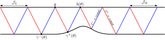
Figure 2. Diagram of $\Omega$. Level lines of $\ell^{+}_{\lambda}$ are in red and level lines of $\ell^{-}_{\lambda}$ are in blue. For a point $\theta\in\partial\Omega_{\uparrow}$, the location of $\gamma^{\pm}(\theta)$ and $b(\theta)$ are indicated. A choice of fundamental intervals $\mathcal{J}_{\mathrm{L}}$ and $\mathcal{J}_{\mathrm{R}}$ is also labeled.

Let us first consider the homogeneous stationary problem

$$P(\lambda)u(x)=0,\quad u|_{\partial\Omega}=0,\quad\lambda\in(0,1)\text{ subcritical.}$$ (1.10)

Near flat ends of the channel, solutions to (1.10) can be expanded as Fourier sine series in $x_{2}$. One can then split the solutions into incoming waves traveling toward the bottom topography and outgoing waves traveling against the bottom topography. Both incoming and outgoing waves can be described in terms of the Neumann data of $u$ on $\mathcal{J}_{\mathrm{L}}$ and $\mathcal{J}_{\mathrm{R}}$. We can then define the scattering matrix that maps the incoming waves to the outgoing waves. More precisely, we show the following. Let $\mathring{L}^{2}(\mathbb{T}_{\lambda})$ consist of $L^{2}$ functions on the torus $\mathbb{T}_{\lambda}$ with zero mean value and let $\Pi^{\pm}$ be the projections onto the positive ($+$) or negative $(-)$ Fourier modes of such a function. We denote $\mathring{H}^{\frac{1}{2}}(\mathbb{T}_{\lambda};T^{*}\mathbb{T}_{\lambda})$ the homogeneous Sobolev space of order $\frac{1}{2}$, consisting of one-forms of mean zero with norms defined by

$$\|\mathbf{g}\|_{\mathring{H}^{\frac{1}{2}}(\mathbb{T}_{\lambda})}=\sum_{k\in\mathbb{Z}}|k||\widehat{\mathbf{g}}(k)|^{2},\ \widehat{\mathbf{g}}(k):=\frac{c(\lambda)}{2\pi}\int_{\mathbb{T}_{\lambda}}e^{-ic(\lambda)k\theta}\mathbf{g}(\theta).$$

See §1.2 for a brief discussion of the notation used for all the Sobolev spaces used in this paper.

Theorem 2.

Suppose $\Omega$ is subcritical for $\lambda\in(0,1)$. Then for any $\mathbf{g}^{i}\in\mathring{L}^{2}(\mathbb{T}_{\lambda})$, there exist unique $\mathbf{g}^{o}\in\mathring{L}^{2}(\mathbb{T}_{\lambda})$ and $u\in\dot{H}^{1}_{\mathrm{loc}}(\Omega)$ such that

$$P(\lambda)u=0,\ \partial_{x_{2}}u|_{\mathcal{J}_{\mathrm{L}}}=\Pi^{+}\mathbf{g}^{i}+\Pi^{-}\mathbf{g}^{o},\ \partial_{x_{2}}u|_{\mathcal{J}_{\mathrm{R}}}=\Pi^{-}\mathbf{g}^{i}+\Pi^{+}\mathbf{g}^{o}.$$

The resulting map

$$\mathbf{S}(\lambda):\mathring{L}^{2}(\mathbb{T}_{\lambda};T^{*}\mathbb{T}_{\lambda})\to\mathring{L}^{2}(\mathbb{T}_{\lambda};T^{*}\mathbb{T}_{\lambda}),\quad\mathbf{g}^{i}\mathrm{d}x_{1}\mapsto\mathbf{g}^{o}\mathrm{d}x_{1},$$

is called the scattering matrix for $P(\lambda)$ in $\Omega$. Moreover, there exists a smoothing operator $R:\mathcal{D}^{\prime}(\mathbb{T}_{\lambda};T^{*}\mathbb{T}_{\lambda})\to C^{\infty}(\mathbb{T}_{\lambda};T^{*}\mathbb{T}_{\lambda})$ such that

$$\mathbf{S}(\lambda)=\Pi^{+}\mathbf{b}_{\lambda}^{*}\Pi^{+}+\Pi^{-}(\mathbf{b}_{\lambda}^{-1})^{*}\Pi^{-}+R.$$

Furthermore, $\mathbf{S}(\lambda)$ has the improved mapping property

$$\mathbf{S}(\lambda):\mathring{H}^{s}(\mathbb{T}_{\lambda};T^{*}\mathbb{T}_{\lambda})\to\mathring{H}^{s}(\mathbb{T}_{\lambda};T^{*}\mathbb{T}_{\lambda})$$ (1.11)

for all $s\in{\mathbb{R}}$ and is in fact a unitary operator on $\mathring{H}^{\frac{1}{2}}(\mathbb{T}_{\lambda})$.

Using the scattering matrix constructed in Theorem 2, one can find purely outgoing solutions (see Definition 1.2 below) to the inhomogeneous stationary problem

$$P(\lambda)u(x)=f(x),\quad u|_{\partial\Omega}=0,\quad\lambda\in(0,1)\text{ subcritical}$$ (1.12)

for given $f\in L^{2}_{\operatorname{comp}}$, $\operatorname{supp}f\subset\overline{\Omega}\cap\{|x_{1}|\leq M\}$. Here $L^{2}_{\operatorname{comp}}(\Omega)$ is the space of compactly supported $L^{2}$ functions on $\overline{\Omega}$. Note that we may always choose $M$ sufficiently large so that this is the same $M$ as in the definition of $\mathcal{J}_{\mathrm{L}}$ and $\mathcal{J}_{\mathrm{R}}$ in (1.9).

Theorem 3.

Suppose $\Omega$ is subcritical for $\lambda\in(0,1)$. Then there exists a map

$$\mathcal{R}(\lambda):L^{2}_{\mathrm{comp}}(\overline{\Omega})\to\dot{H}^{1}_{\mathrm{loc}}(\Omega)$$

such that for any $f\in L^{2}_{\mathrm{comp}}(\overline{\Omega})$, the function $u:=\mathcal{R}(\lambda)f$ is the unique solution to (1.12) satisfying

$$\Pi^{+}(\partial_{x_{2}}u|_{\mathcal{J}_{\mathrm{L}}})=\Pi^{-}(\partial_{x_{2}}u|_{\mathcal{J}_{\mathrm{R}}})=0.$$

Moreover,

$$\mathcal{R}(\lambda):\bar{H}^{s}_{\operatorname{comp}}(\Omega)\to\dot{H}^{1}_{\operatorname{loc}}(\Omega)\cap\bar{H}^{s+1}_{\operatorname{loc}}(\omega),\quad s\geq 0,$$

and for any $\delta>0$, if $f\in\bar{H}^{\delta}(\Omega)$ and $u_{\lambda-i\varepsilon}$ solves (1.4) with $\omega=\lambda-i\varepsilon$, $\varepsilon>0$, then for any $\chi\in C^{\infty}_{c}(\overline{\Omega})$,

$$\chi u_{\lambda-i\varepsilon}\to\chi\mathcal{R}(\lambda)f\text{ in }\bar{H}^{1}(\Omega)\text{ as }\varepsilon\to 0+.$$

We make the following definition for incoming and outgoing solutions. This definition is analogous to incoming an outgoing solutions in Euclidean scattering in view of the limiting absorption principle that we will establish in Proposition 4.5.

Definition 1.2.

A solution to (1.12) satisfying conditions in Theorem 3 is called outgoing. A solution $u$ to (1.12) is called incoming if

$$\Pi^{-}(\partial_{x_{2}}u|_{\mathcal{J}_{\mathrm{L}}})=\Pi^{+}(\partial_{x_{2}}u|_{\mathcal{J}_{\mathrm{R}}})=0.$$

The Poincaré problem (1.1) will be analyzed with the help of Theorems 2 and 3. In particular, we show in Theorem 1 that the leading profile in the long time evolution is a standing wave whose spatial component is precisely $\mathcal{R}(\lambda)f$ constructed in Theorem 3.

1.1. Relation to the oceanographic literature

The oceanographic literature contains some explorations of the scattering problem as discussed here (it is of considerable importance, e.g., in the study of mixing in the ocean [ML00b]). Longuet-Higgins [LH69], for example, considers the approximation to the scattering given by ray-tracing, as motivated by WKB solutions. This was clearly understood as a high-frequency approximation: Müller–Liu [ML00a, §5c] note that “One expects reflection theory to do the worst for low incident modenumbers. This is indeed the case.” Indeed, Baines [Bai71] performed a more refined analysis of plane-wave scattering that involved a Fredholm integral operator correcting the ray tracing approximation, which he too noted is inaccurate, especially at low wavenumbers. Baines worked in an ocean with no surface, however, rather than the finite channel under consideration here. Our approach is morally similar, but involves rigorous discussion of uniqueness of outgoing solutions, the derivation of the limiting absorption principle, and an analysis of the consequences of the spectral analysis for the time-domain forced problem. Our results on the scattering matrix quantitatively justify the assertion that the reflection theory approximates the scattering matrix, by showing that the error in this approximation is rapidly decaying in the wavenumber parameter.

1.2. Some Sobolev spaces

Before moving on, we quickly fix the notation for various Sobolev spaces on manifolds with boundary. If $F\subset\mathcal{D}^{\prime}({\mathbb{R}}^{2})$ is a closed linear subspace of Schwartz distributions, we denote by $\dot{F}(\Omega)\subset F$ the subspace of $F$ supported on $\overline{\Omega}$, and $\bar{F}(\Omega)=F/\dot{F}({\mathbb{R}}^{2}\setminus\Omega)$ the space of extendable distributions on $\Omega$. For instance, $\dot{H}^{1}(\Omega)$ denotes the set of functions in $H^{1}({\mathbb{R}}^{2})$ whose support lies in $\overline{\Omega}$. In particular, $\dot{H}^{1}(\Omega)\simeq H^{1}_{0}(\Omega)$, where $H^{1}_{0}(\Omega)$ denotes the usual space of trace-free $H^{1}$ functions on $\Omega$. We also remark that $\dot{L}^{2}(\Omega)=\bar{L}^{2}(\Omega)=L^{2}(\Omega)$. For more details, see [Hör85, Appendix B]. We will also use the subscripts $\operatorname{loc}$ or $\operatorname{comp}$ to denote local and compactly supported Sobolev spaces respectively. Finally, we denote by $\mathring{H}^{s}(\mathbb{T};T^{*}\mathbb{T})$ to be the subset of distributional one-forms $\mathbf{v}\in H^{s}(\mathbb{T};T^{*}\mathbb{T})$ such that $\int\mathbf{v}=0$.

Acknowledgments. The authors would like to thank Semyon Dyatlov for helpful discussions. J. Wunsch acknowledges partial support from NSF grant DMS–2054424 and from Simons Foundation Grant MPS-TSM-00007464. Z. Li acknowledges partial support from Semyon Dyatlov’s NSF grant DMS–2400090.

2. Solutions to the stationary problem

We study the stationary problem (1.12) in this section. Let us start by introducing coordinates $y_{\pm}:=\ell_{\lambda}^{\pm}(x)$, where $\ell^{\pm}$ were defined in (1.5). In these coordinates, we have

$$P(\lambda)=\tfrac{1}{4}\partial_{y_{+}}\partial_{y_{-}}.$$

The upper boundary is given by

$$\partial\Omega_{\uparrow}=\{(y_{+},y_{-})\mid y_{+}+y_{-}=0\}$$

and we parametrize $\partial\Omega_{\uparrow}$ by

$$\mathbf{y}:{\mathbb{R}}\to\partial\Omega_{\uparrow},\ \theta\mapsto\left(\frac{\theta}{\sqrt{1-\lambda^{2}}},-\frac{\theta}{\sqrt{1-\lambda^{2}}}\right).$$ (2.1)

Note that under this parametrization, there exists $M>0$ depending on the topography $G$ such that

$$b_{\lambda}(\theta)=\theta+2\pi\text{ for all }|\theta|\geq M.$$

We use $\mathcal{J}_{\pm}$ to denote the pre-image of the left/right fundamental intervals defined in §1 when there is no ambiguity.

2.1. Compactly supported inhomogeneity

Working in $(y_{+},y_{-})$ coordinates, we see that (1.12) becomes

$$\partial_{y_{+}}\partial_{y_{-}}u=4f,\ u|_{\partial\Omega}=0.$$

We define

$$U_{0}(y_{+},y_{-}):=4\int_{-\infty}^{y_{+}}\int_{-\infty}^{y_{-}}f(s_{+},s_{-})\mathrm{d}s_{+}\mathrm{d}s_{-}.$$ (2.2)

Since $f\in L^{2}_{\mathrm{comp}}(\overline{\Omega})$, we know $U_{0}$ is defined for all $(y_{+},y_{-})\in\Omega$. Moreover,

$$P(\lambda)U_{0}=f,\ U_{0}\in H^{1}_{\mathrm{comp}}(\overline{\Omega}),\ U_{0}|_{\partial\Omega_{\downarrow}}=0,\ g:=U_{0}|_{\partial\Omega_{\uparrow}}\in H^{1}_{\mathrm{comp}}(\partial\Omega_{\uparrow}).$$ (2.3)

Note that a priori, restricting $U_{0}$ to boundary should only yield an $L^{2}$ function on the boundary. However, we deduce from (2.2) that in fact the restriction to boundary lies in $H^{1}({\mathbb{R}})$. Furthermore, observe that if $u\in\bar{H}^{s}_{\operatorname{comp}}(\Omega)$, $s\geq 0$, then $U_{0}\in\bar{H}^{s+1}_{\operatorname{comp}}(\Omega)$, which means $g\in H^{s}_{\operatorname{comp}}(\partial\Omega_{\uparrow})$.

Now to solve $u$ in (1.12), one only needs to solve for $w:=U_{0}-u$ that satisfies the homogeneous boundary value equation

$$\partial_{y_{+}}\partial_{y_{-}}w=0,\quad w|_{\partial\Omega_{\downarrow}}=0,\quad w|_{\partial\Omega_{\uparrow}}=g\in H^{1}_{\operatorname{comp}}(\partial\Omega_{\uparrow})$$ (2.4)

Lemma 2.1.

Suppose $\Omega$ is subcritical for $\lambda\in(0,1)$ and $w\in\dot{H}^{1}_{\mathrm{loc}}(\Omega)$ solves (2.4). Then there exist $w_{\pm}\in\dot{H}^{1}_{\mathrm{loc}}({\mathbb{R}})$ such that

$$w(y_{+},y_{-})=w_{+}(y_{+})+w_{-}(y_{-}).$$

Proof.

Define $w_{+}^{1}:=\partial_{y_{+}}w$. Then we know

$$w_{+}^{1}\in L^{2}_{\mathrm{loc}}(\Omega),\ \partial_{y_{-}}w_{+}^{1}=0.$$

The second equation together with the assumption that $\Omega$ is subcritical shows that $w_{+}^{1}$ depends only on $y_{+}$. Since $y_{+}$ can take any value in ${\mathbb{R}}$, we know $w_{+}^{1}$ defines a function on ${\mathbb{R}}$. For every $a>0$, there exists $\delta>0$ such that the parallelogram $\Omega_{a,\delta}:=\{(y_{+},y_{-})\mid|y_{+}|\leq a,\ -y_{+}-\delta\leq y_{-}\leq-y_{+}\}$ is a subset of $\Omega$. Thus we see that

$$\|w_{+}^{1}\|_{L^{2}([-a,a])}^{2}\leq\delta^{-1}\|\partial_{y_{+}}w\|_{L^{2}(\Omega_{a,\delta})}^{2}\leq\delta^{-1}\|w\|_{H^{1}(\Omega_{a,\delta})}^{2}<\infty.$$

This shows that $w_{+}^{1}\in L^{2}_{\mathrm{loc}}({\mathbb{R}})$. Define

$$w_{+}(y_{+}):=\int_{0}^{y_{+}}w_{+}^{1}(s)\mathrm{d}s.$$

Then $w_{+}$ satisfies

$$w_{+}\in H^{1}_{\mathrm{loc}}({\mathbb{R}}),\ \partial_{y_{+}}(w(y_{+},y_{-})-w_{+}(y_{+}))=0.$$

This shows that $w_{-}:=w-w_{+}$ is a function depending only on $y_{-}$. Moreover, $\partial_{y_{-}}w_{-}=\partial_{y_{-}}w$. Similar argument as above shows that $w_{-}\in H^{1}_{\mathrm{loc}}({\mathbb{R}})$. ∎

By abuse of notation, we also denote the pullbacks $y_{\pm}^{*}w_{\pm}$ by $w_{\pm}$, where $y_{\pm}^{*}$ denote projections $(y_{+},y_{-})\mapsto y_{\pm}$, so that $w_{\pm}$ can be viewed as elements of $\bar{H}^{1}_{\operatorname{loc}}(\Omega)$. In this sense, $w_{\pm}$ can be restricted to $\partial\Omega$, and the restrictions lie in $H^{1}_{\mathrm{loc}}(\partial\Omega)$. Note that

$$w_{\pm}|_{\partial\Omega}=(\gamma^{\pm})^{*}(w_{\pm}|_{\partial\Omega})$$

by (1.7). Applying the boundary conditions in (2.4) we have

$$w_{+}|_{\partial\Omega_{\uparrow}}+w_{-}|_{\partial\Omega_{\uparrow}}=g,\ w_{+}|_{\partial\Omega_{\downarrow}}+w_{-}|_{\partial\Omega_{\downarrow}}=0.$$

Therefore, using the $\mathbf{y}$ parametrization (2.1) of $\partial\Omega_{\uparrow}$, we have

$$\begin{split}w_{\pm}|_{\partial\Omega_{\uparrow}}(\theta)=&w_{\pm}|_{\partial\Omega_{\downarrow}}(\gamma^{\pm}(\theta))=-w_{\mp}|_{\partial\Omega_{\downarrow}}(\gamma^{\pm}(\theta))=-w_{\mp}|_{\partial\Omega_{\uparrow}}(\gamma^{\mp}\circ\gamma^{\pm}(\theta))\\ =&-w_{\mp}|_{\partial\Omega_{\uparrow}}(b^{\pm 1}(\theta))=w_{\pm}|_{\partial\Omega_{\uparrow}}(b^{\pm 1}(\theta))-g(b^{\pm 1}(\theta)).\end{split}$$

That is,

$$w_{\pm}|_{\partial\Omega_{\uparrow}}-(b^{\pm 1})^{*}(w_{\pm}|_{\partial\Omega_{\uparrow}})=-(b^{\pm 1})^{*}g.$$ (2.5)

Iterate (2.5) $N$ times, restrict $w_{+}$ to the left/right fundamental intervals $\mathcal{J}_{\mathrm{L}}$, $\mathcal{J}_{\mathrm{R}}$ (see §1), then differentiate both sides, and we find

$$\mathbf{v}_{\mathrm{L}}-\mathbf{b}^{*}\mathbf{v}_{\mathrm{R}}=\mathbf{g}.$$ (2.6)

Here $\mathbf{b}=b_{\lambda}^{N}$ is the multi-bounce chess billiard map defined in §1 (we now suppress the $\lambda$ subscript) and

$$\begin{split}\mathbf{v}_{\bullet}:=&\mathrm{d}w_{+}|_{\mathcal{J}_{\bullet}}\in\mathring{L}^{2}(\mathcal{J}_{\bullet};T^{*}\mathcal{J}_{\bullet}),\quad\bullet=\mathrm{L},\mathrm{R},\\ \mathbf{g}:=&-\sum_{k=1}^{N}(b^{k})^{*}\mathrm{d}g|_{\mathcal{J}_{\mathrm{L}}}\in\mathring{L}^{2}(\mathcal{J}_{\mathrm{L}};T^{*}\mathcal{J}_{\mathrm{L}}).\end{split}$$ (2.7)

Let us take a step back and interpret all the new objects we have defined. We claim that $\mathbf{v}_{\mathrm{L}}$ and $\mathbf{v}_{\mathrm{R}}$ are essentially the Neumann data of the solution $u$ on $\mathcal{J}_{\mathrm{L}}$, $\mathcal{J}_{\mathrm{R}}$ respectively.

Lemma 2.2.

Suppose $u\in\dot{H}^{1}_{\operatorname{loc}}$ satisfies the stationary internal wave equation (1.12). Then

$$v_{\uparrow}:=\mathbf{j}^{*}(\partial_{y_{+}}u\,\mathrm{d}y_{+})$$

is well-defined in $L^{2}_{\mathrm{comp}}(\partial\Omega_{\uparrow};T^{*}\partial\Omega_{\uparrow})$, where $\mathbf{j}:\partial\Omega_{\uparrow}\to{\mathbb{R}}^{2}$ is the canonical embedding. Furthermore,

$$\mathbf{v}_{\bullet}=-v_{\uparrow}|_{\mathcal{J}_{\bullet}},\ \bullet=\mathrm{L},\mathrm{R}$$

where $\mathbf{v}_{\mathrm{L}}$ and $\mathbf{v}_{\mathrm{R}}$ are as defined in (2.7).

Remark. It is easy to check that in the $x_{1}$ coordinates on $\partial\Omega$, $v_{\uparrow}$ is given by

$$v_{\uparrow}=\tfrac{1}{2}\partial_{x_{2}}u|_{\partial\Omega_{\uparrow}}\mathrm{d}x_{1}.$$

Therefore, $\mathbf{v}_{\mathrm{L}}$ and $\mathbf{v}_{\mathrm{R}}$ are simply a multiple of the Neumann data.

Proof.

Recall that

$$u=U_{0}-(w_{+}+w_{-})$$

where $w_{\pm}$ depends only on $y_{\pm}$. Therefore,

$$\partial_{y_{+}}u(y_{+},y_{-})\mathrm{d}y_{+}=\partial_{y_{+}}U_{0}(y_{+},y_{-})\mathrm{d}y_{+}-\mathrm{d}w_{+}.$$

Since $U_{0}\in H^{1}_{\mathrm{comp}}(\overline{\Omega})$, it follows that $v_{\uparrow}$ is well-defined in $L^{2}_{\mathrm{comp}}$. The relationship to $\mathbf{v}_{\mathrm{L}}$ and $\mathbf{v}_{\mathrm{R}}$ follows from the fact that $U_{0}$ vanishes in a neighborhood of $\mathcal{J}_{\mathrm{L}}\cup\mathcal{J}_{\mathrm{R}}.$∎

Motivated by the above lemma, we call $\mathbf{v}_{\mathrm{L}}$ and $\mathbf{v}_{\mathrm{R}}$ the Neumann data at left and right infinity respectively. Next, we retrace our steps and verify that if (2.6) is satisfied, we indeed have a solution with the given Neumann data.

Lemma 2.3.

Assume that $f\in\bar{H}^{s}_{\operatorname{comp}}$ for some $s\geq 0$. Let $\mathbf{v}_{\mathrm{L}}\in\mathring{H}^{s}(\mathcal{J}_{\mathrm{L}};T^{*}\mathcal{J}_{\mathrm{L}})$ and $\mathbf{v}_{\mathrm{R}}\in\mathring{H}^{s}(\mathcal{J}_{\mathrm{R}};T^{*}\mathcal{J}_{\mathrm{R}})$. If $\mathbf{v}_{\mathrm{L}}$ and $\mathbf{v}_{\mathrm{R}}$ satisfies (2.6), then there exists $u\in\dot{H}^{1}_{\operatorname{loc}}(\Omega)\cap\bar{H}^{s+1}_{\operatorname{loc}}(\Omega)$ that satisfies (1.12) with $\mathbf{v}_{\mathrm{L}}$ and $\mathbf{v}_{\mathrm{R}}$ as the Neumann data on the left and the right fundamental intervals respectively.

Proof.

Let $U_{0}$ and $g$ be as defined in (2.2) and (2.3). Let $\mathcal{J}_{\mathrm{L}}=[\theta_{0},\theta_{0}+2\pi)$ be the left fundamental interval defined in (1.9) using the parametrization $\mathbf{y}$ defined in (2.1). Notice that $b^{k}(\mathcal{J}_{\mathrm{L}})$, $k\in\mathbb{Z}$, tiles $\partial\Omega_{\uparrow}$. Then we can define a function $\omega$ on $\partial\Omega_{\uparrow}$ by

$$\omega|_{\mathcal{J}_{\mathrm{L}}}(\theta):= \int_{\theta_{0}}^{\theta}\mathbf{\mathbf{v}_{\mathrm{L}}},$$ (2.8)

$$\omega|_{b^{k}(\mathcal{J}_{\mathrm{L}})}:= (b^{-k})^{*}(\omega|_{\mathcal{J}_{\mathrm{L}}}),$$

$$\omega|_{b^{-k}(\mathcal{J}_{\mathrm{L}})}:= (b^{k})^{*}(\omega|_{\mathcal{J}_{\mathrm{L}}})-\sum_{n=1}^{k}(b^{n})^{*}g|_{b^{-k}(\mathcal{J}_{\mathrm{L}})},\ k\geq 1.$$

One can check that $\omega$ satisfies

$$\omega-b^{*}\omega=-b^{*}g.$$ (2.9)

Note that since $f\in\bar{H}^{s}_{\operatorname{comp}}$, we have $g\in H_{\operatorname{comp}}^{s+1}(\partial\Omega_{\uparrow})$. Combined with the assumption that $\int\mathbf{v}_{\mathrm{L}}=0$, it follows that $\omega$ is in fact continuous on the circle, as well as lying in $H^{s+1}_{\operatorname{loc}}(\partial\Omega_{\uparrow})$. Observe that there exist unique $w_{\pm}\in\bar{H}^{s+1}_{\operatorname{loc}}(\Omega)$ such that for $(y_{+},y_{-})\in\Omega$,

$$w_{+}(y_{+},y_{-}) :=\omega(\theta),\text{ when }y_{+}=y_{+}(\theta),$$ (2.10)

$$w_{-}(y_{+},y_{-}) :=g(\theta)-\omega(\theta),\text{ when }y_{-}=y_{-}(\theta)$$

where $\mathbf{y}(\theta)=(y_{+}(\theta),y_{-}(\theta))$. We claim that

$$u:=U_{0}-(w_{+}+w_{-})$$

is our desired solution. Clearly, $P(\lambda)u=f$, $u\in\bar{H}^{1}_{\operatorname{loc}}(\Omega)$, and $u|_{\partial\Omega_{\uparrow}}=0$. Since

$$(\gamma^{+})^{*}w_{+}(y_{+})=w_{+}(y_{+}),$$

while

$$(\gamma^{+})^{*}w_{-}(y_{-})=w_{-}(y_{-}\circ\gamma^{+})=w_{-}(y_{-}\circ\gamma^{-}\circ\gamma^{+})=b^{*}w_{-}(y_{-}),$$

the relations (2.10) together with (2.9) yield

$$(\gamma^{+})^{*}(u|_{\partial\Omega_{\downarrow}})=0-(\omega+(b^{*}g-b^{*}\omega))=0.$$

Since $(\gamma^{+})^{2}=\mathrm{Id}$, we conclude that $u|_{\partial\Omega_{\downarrow}}=0$. Thus we have $u\in\dot{H}^{1}_{\operatorname{loc}}(\Omega)\cap\bar{H}^{s+1}_{\operatorname{loc}}(\Omega)$. Finally, by the second equation in (2.8) with $k=N$, the right Neumann data of the solution $u$ is precisely given by $\mathbf{v}_{\mathrm{R}}$ satisfying the relation (2.6). ∎

2.2. Schwartz class inhomogeneity

To obtain a limiting absorption principle later in §4.2, it turns out that we also need to consider (1.12) with the right-hand-side in Schwartz class rather than having compact support. More explicitly, we study

$$P(\lambda)u(x)=f(x),\ u|_{\partial\Omega}=0,\quad f\in\overline{\mathscr{S}}(\Omega).$$ (2.11)

Again working in $(y_{+},y_{-})$ coordinates, we see that the reduction to a homogeneous boundary value problem in (2.2)-(2.3) holds identically for $f\in\overline{\mathscr{S}}(\Omega)$. Then the corresponding modification of (2.4) for the Schwartz inhomogeneity (2.11) is given by

$$\partial_{y_{+}}\partial_{y_{-}}w=0,\quad w|_{\partial\Omega_{\downarrow}}=0,\quad w|_{\partial\Omega_{\uparrow}}=g\in\mathscr{S}(\partial\Omega_{\uparrow}),$$ (2.12)

with the only change being the regularity of $g$. One can readily check that Lemma 2.1 holds for (2.12) instead of (2.4).

The primary modification that needs to be made to §2.1 to the Schwartz inhomogeneity case is in the definition of $\mathbf{v}_{\mathrm{L}}$, $\mathbf{v}_{\mathrm{R}}$, and $\mathbf{g}$. The reason is that $g$ is no longer compactly supported and its effects extend out to left and right infinity, so simply restricting to the left and right fundamental intervals no longer captures the Neumann data near left and right infinity. However, since $g$ is Schwartz, its effects near infinity are very weak. The adjustment we will make simply pulls back data at left and right infinity to the left and right fundamental intervals. Define

$$\begin{split}\mathbf{v}_{\mathrm{L}}:=&\lim_{k\to\infty}((b^{-k})^{*}\mathrm{d}w_{+})|_{\mathcal{J}_{\mathrm{L}}}\in\mathring{L}^{2}(\mathcal{J}_{\mathrm{L}};T^{*}\mathcal{J}_{\mathrm{L}}),\\ \mathbf{v}_{\mathrm{R}}:=&\lim_{k\to\infty}((b^{k})^{*}\mathrm{d}w_{+})|_{\mathcal{J}_{\mathrm{R}}}\in\mathring{L}^{2}(\mathcal{J}_{\mathrm{R}};T^{*}\mathcal{J}_{\mathrm{R}}),\\ \mathbf{g}:=&\sum_{k\in\mathbb{Z}}((b^{k})^{*}\mathrm{d}g)|_{I_{L}}\in\mathring{C}^{\infty}(\mathcal{J}_{\mathrm{L}};T^{*}\mathcal{J}_{\mathrm{L}}).\end{split}$$ (2.13)

The limits exist since $g\in\mathscr{S}(\partial\Omega_{\uparrow})$. Note that if $g\in L^{2}_{\operatorname{comp}}$, then the definitions in (2.13) coincide with (2.7). Furthermore, it is easy to verify that (2.6) still holds with the new definitions in (2.13). Now we have the following analogue of Lemma 2.3.

Lemma 2.4.

Assume that $f\in\overline{\mathscr{S}}(\Omega)$. Let $\mathbf{v}_{\mathrm{L}}\in\mathring{H}^{s}(\mathcal{J}_{\mathrm{L}};T^{*}\mathcal{J}_{\mathrm{L}})$ and $\mathbf{v}_{\mathrm{R}}\in\mathring{H}^{s}(\mathcal{J}_{\mathrm{R}};T^{*}\mathcal{J}_{\mathrm{R}})$ for some $s\geq 0$. If $\mathbf{v}_{\mathrm{L}}$ and $\mathbf{v}_{\mathrm{R}}$ satisfies (2.6), then there exists $u\in\dot{H}^{1}_{\operatorname{loc}}\cap\bar{H}^{s+1}_{\operatorname{loc}}$ that satisfies (1.12) with $\mathbf{v}_{\mathrm{L}}$ and $\mathbf{v}_{\mathrm{R}}$ as the Neumann data on the left and the right fundamental intervals respectively.

Proof.

We simply need to take into account the mild effects of $g$ near left and right infinity in the proof of Lemma 2.3. In particular, we modify the definition of $\omega$ in (2.8), and define instead

$$\omega|_{\mathcal{J}_{\mathrm{L}}}(\theta):= -\sum_{n=0}^{\infty}((b^{-n})^{*}g)|_{\mathcal{J}_{\mathrm{L}}}(\theta)+\int_{\theta_{0}}^{\theta}\mathbf{v}_{\mathrm{L}},$$

$$\omega|_{b^{k}(\mathcal{J}_{\mathrm{L}})}:= (b^{-k})^{*}(\omega|_{\mathcal{J}_{\mathrm{L}}})+\sum_{n=0}^{k-1}(b^{-n})^{*}g|_{b^{k}(\mathcal{J}_{\mathrm{L}})},\ k\geq 1,$$

$$\omega|_{b^{-k}(\mathcal{J}_{\mathrm{L}})}:= (b^{k})^{*}(\omega|_{\mathcal{J}_{\mathrm{L}}})-\sum_{n=1}^{k}(b^{n})^{*}g|_{b^{-k}(\mathcal{J}_{\mathrm{L}})},\ k\geq 1.$$

The rest of the proof of Lemma 2.3 holds verbatim. ∎

We define the analogue to Definition 1.2 for incoming and outgoing solution to the case of Schwartz inhomogeneity.

Definition 2.5.

Let $u$ be a solution to (2.11) and let $\mathbf{v}_{\mathrm{L}}$ and $\mathbf{v}_{\mathrm{R}}$ be the Neumann data near left and right infinity defined in (2.13). Then we call

$$(\Pi^{-}\mathbf{v}_{\mathrm{L}},\Pi^{+}\mathbf{v}_{\mathrm{R}})$$

the outgoing data, and

$$(\Pi^{+}\mathbf{v}_{\mathrm{L}},\Pi^{-}\mathbf{v}_{\mathrm{L}})$$

the incoming data. $u$ is called outgoing if the incoming data vanishes, and incoming if the outgoing data vanishes.

Note that these definitions are consistent with Definition 1.2, in the sense that the two definitions agree if $u$ is a solution to (1.12).

3. Scattering matrix

We now consider the homogeneous stationary internal wave equation (1.10) (or (2.11) for Schwartz inhomogeneity). Then the left and right Neumann data defined in (2.7) (or (2.13) for Schwartz inhomogeneity) satisfies

$$\mathbf{v}_{\mathrm{L}}-\mathbf{b}^{*}\mathbf{v}_{\mathrm{R}}=0.$$

Using the parametrization $\mathbf{y}$ in §2, we can identify $\mathcal{J}_{\mathrm{L}}$ and $\mathcal{J}_{\mathrm{R}}$ with $\mathbb{S}^{1}={\mathbb{R}}/2\pi\mathbb{Z}$ so that $\mathbf{v}_{\mathrm{L}},\mathbf{v}_{\mathrm{R}}\in\mathring{L}^{2}(\mathbb{S}^{1};T^{*}\mathbb{S}^{1})$ and $\mathbf{b}\in C^{\infty}(\mathbb{S}^{1};\mathbb{S}^{1})$. Then taking the positive and negative Fourier projectors $\Pi^{\pm}$, the outgoing data can be expressed as

$$\begin{split}\begin{pmatrix}\Pi^{-}\mathbf{v}_{\mathrm{L}}\\ \Pi^{+}\mathbf{v}_{\mathrm{R}}\end{pmatrix}=&\begin{pmatrix}\Pi^{-}\mathbf{b}^{*}\mathbf{v}_{\mathrm{R}}\\ \Pi^{+}\mathbf{b}^{-*}\mathbf{v}_{\mathrm{L}}\end{pmatrix}\\ =&\begin{pmatrix}0&\Pi^{+}\mathbf{b}^{*}\Pi^{-}\\ \Pi^{-}\mathbf{b}^{*}\Pi^{+}&0\end{pmatrix}\begin{pmatrix}\Pi^{-}\mathbf{v}_{\mathrm{L}}\\ \Pi^{+}\mathbf{v}_{\mathrm{R}}\end{pmatrix}+\begin{pmatrix}\Pi^{-}\mathbf{b}^{*}\Pi^{-}&0\\ 0&\Pi^{+}\mathbf{b}^{-*}\Pi^{+}\end{pmatrix}\begin{pmatrix}\Pi^{-}\mathbf{v}_{\mathrm{R}}\\ \Pi^{+}\mathbf{v}_{\mathrm{L}}\end{pmatrix}\end{split}$$

where $\mathbf{b}^{-*}:=(\mathbf{b}^{-1})^{*}$. We rewrite the equation as

$$\begin{pmatrix}\mathrm{Id}&-\Pi^{+}\mathbf{b}^{*}\Pi^{-}\\ -\Pi^{-}\mathbf{b}^{*}\Pi^{+}&\mathrm{Id}\end{pmatrix}\begin{pmatrix}\Pi^{-}\mathbf{v}_{\mathrm{L}}\\ \Pi^{+}\mathbf{v}_{\mathrm{R}}\end{pmatrix}=\begin{pmatrix}\Pi^{-}\mathbf{b}^{*}\Pi^{-}&0\\ 0&\Pi^{+}\mathbf{b}^{-*}\Pi^{+}\end{pmatrix}\begin{pmatrix}\Pi^{-}\mathbf{v}_{\mathrm{R}}\\ \Pi^{+}\mathbf{v}_{\mathrm{L}}\end{pmatrix}.$$ (3.1)

Our goal is to recover the outgoing data $\begin{pmatrix}\Pi^{-}\mathbf{v}_{\mathrm{L}}\\ \Pi^{+}\mathbf{v}_{\mathrm{R}}\end{pmatrix}$ in terms of the incoming data $\begin{pmatrix}\Pi^{-}\mathbf{v}_{\mathrm{R}}\\ \Pi^{+}\mathbf{v}_{\mathrm{L}}\end{pmatrix}$ , so it suffices to invert

$$\begin{gathered}\mathbf{T}:\Pi^{-}L^{2}(\mathbb{S}^{1};T^{*}\mathbb{S}^{1})\times\Pi^{+}L^{2}(\mathbb{S}^{1};T^{*}\mathbb{S}^{1})\to\Pi^{-}L^{2}(\mathbb{S}^{1};T^{*}\mathbb{S}^{1})\times\Pi^{+}L^{2}(\mathbb{S}^{1};T^{*}\mathbb{S}^{1}),\\ \mathbf{T}:=\begin{pmatrix}\operatorname{Id}&-\Pi^{-}\mathbf{b}^{*}\Pi^{+}\\ -\Pi^{+}\mathbf{b}^{-*}\Pi^{-}&\operatorname{Id}\end{pmatrix}.\end{gathered}$$

To do so, we need the following lemma.

Lemma 3.1.

Let $\varphi$ be an orientation-preserving diffeomorphism of $\mathbb{S}^{1}$ and let $v\in L^{2}(\mathbb{S}^{1};T^{*}\mathbb{S}^{1})$. Then

$$\Pi^{-}\varphi^{*}\Pi^{-}v=0\text{ implies }\Pi^{-}v=0.$$

Proof.

Assume for the sake of contradiction that $\Pi^{-}v\neq 0$ and

$$\Pi^{-}\varphi^{*}\Pi^{-}v=0,$$

hence

$$\varphi^{*}\Pi^{-}v=(I-\Pi^{-})\varphi^{*}\Pi^{-}v.$$ (3.2)

The operator on the right-hand-side of (3.2) is a smoothing operator (by the calculus of wavefront sets, using the fact that $\varphi$ is orientation-preserving), hence $\varphi^{*}\Pi^{-}v\in C^{\infty}(\mathbb{S}^{1};T^{*}\mathbb{S}^{1})$. Thus also $\Pi^{-}v\in C^{\infty}(\mathbb{S}^{1};T^{*}\mathbb{S}^{1}).$

Note that $\int\Pi^{-}v=0$. We can then define the function

$$w(\theta)=\int_{0}^{\theta}\Pi^{-}v\in C^{\infty}(\mathbb{S}^{1}).$$

Clearly, $\widehat{w}(k):=\frac{1}{2\pi}\int_{\mathbb{S}^{1}}e^{-ik\theta}w(\theta)\,d\theta=0$ for all $k>0$. Therefore,

$$\mathbf{F}(w):=\frac{1}{i}\int_{\mathbb{S}^{1}}\overline{w}\mathrm{d}w=2\pi\sum_{k\leq 0}k|\widehat{w}(k)|^{2}<0.$$

Note that $\mathbf{F}(w)=\mathbf{F}(\varphi^{*}w)$. Therefore, there exist $k_{-}<0$ such that $\widehat{\varphi^{*}w}(k_{-})\neq 0$. Since

$$\varphi^{*}\Pi^{-}v=\mathrm{d}\varphi^{*}w$$

it follows that $\widehat{\varphi^{*}\Pi^{-}v}(k_{-})\neq 0$, which contradicts $\Pi^{-}\varphi^{*}\Pi^{-}v=0$. Therefore we must have $\Pi^{-}v=0$. ∎

Now it follows that $\mathbf{T}$ is invertible.

Lemma 3.2.

The nullspace of $\mathbf{T}$ on $\Pi^{-}L^{2}(\mathbb{S}^{1};T^{*}\mathbb{S}^{1})\times\Pi^{+}L^{2}(\mathbb{S}^{1};T^{*}\mathbb{S}^{1})$ is trivial.

Proof.

Let $\begin{pmatrix}v_{-}\\ v_{+}\end{pmatrix}\in\Pi^{-}L^{2}(\mathbb{S}^{1};T^{*}\mathbb{S}^{1})\times\Pi^{+}L^{2}(\mathbb{S}^{1};T^{*}\mathbb{S}^{1})$ be such that $\mathbf{T}\begin{pmatrix}v_{-}\\ v_{+}\end{pmatrix}=0$. Then we must have

$$v_{-}=\Pi^{-}\mathbf{b}^{*}\Pi^{+}\mathbf{b}^{-*}\Pi^{-}v_{-}.$$

Let $v:=\mathbf{b}^{-*}\Pi^{-}v_{-}$. Then $v_{-}=\Pi^{-}\mathbf{b}^{*}\Pi^{+}v$, from which we see that

$$\Pi^{-}\mathbf{b}^{*}v=\Pi^{-}\mathbf{b}^{*}(\mathbf{b}^{-*}\Pi^{-}v_{-})=\Pi^{-}v_{-}=\Pi^{-}\mathbf{b}^{*}\Pi^{+}v.$$ (3.3)

Note that the zeroth Fourier coefficient of $v$ vanishes since $\mathbf{b}^{*}$ is the pullback on 1-forms, so $v-\Pi^{+}v=\Pi^{-}v$. Then it follows from (3.3) that

$$\Pi^{-}\mathbf{b}^{*}\Pi^{-}v=0.$$

By Lemma 3.1, it follows that $\Pi^{-}v=0$. In particular, this means that $\Pi^{-}\mathbf{b}^{-*}\Pi^{-}v_{-}=0$. Apply Lemma 3.1 again, and we see that $v_{-}=\Pi^{-}v_{-}=0$. A similar argument shows that $v_{+}=0$, so the nullspace is indeed trivial. ∎

Let us now complete the proof of Theorem 2.

Proof.

Suppose $\mathbf{g}^{i}\in\mathring{L}^{2}(\mathbb{T}_{\lambda})$. We regard $\mathbf{g}^{i}$ as an element in $\Pi^{-}L^{2}(\mathbb{S}^{1};T^{*}\mathbb{S}^{1})\times\Pi^{+}L^{2}(\mathbb{S}^{1};T^{*}\mathbb{S}^{1})$ through

$$\begin{split}\mathbf{g}^{i}\mapsto(\mathbf{y}^{*}(\Pi^{-}\mathbf{g}^{i}\mathrm{d}x_{1}),\mathbf{y}^{*}(\Pi^{+}\mathbf{g}^{i}\mathrm{d}x_{1}))=:(\mathbf{g}^{i}_{\mathrm{R}},\mathbf{g}^{i}_{\mathrm{L}}).\end{split}$$

By Lemma 3.2, we can define $(\mathbf{g}^{o}_{\mathrm{L}},\mathbf{g}^{o}_{\mathrm{R}})$ and $\mathbf{g}^{o}$ such that

$$\begin{pmatrix}\mathbf{g}^{o}_{\mathrm{L}}\\ \mathbf{g}^{o}_{\mathrm{R}}\end{pmatrix}:=\mathbf{T}^{-1}\begin{pmatrix}\Pi^{-}\mathbf{b}^{*}\Pi^{-}&0\\ 0&\Pi^{+}\mathbf{b}^{-*}\Pi^{+}\end{pmatrix}\begin{pmatrix}\mathbf{g}^{i}_{\mathrm{R}}\\ \mathbf{g}^{i}_{\mathrm{L}}\end{pmatrix},\ \mathbf{g}^{o}:=\mathbf{g}^{o}_{\mathrm{L}}+\mathbf{g}^{o}_{\mathrm{R}}.$$

Define

$$\mathbf{v}_{\mathrm{L}}:=\mathbf{g}^{i}_{\mathrm{L}}+\mathbf{g}^{o}_{\mathrm{L}},\ \mathbf{v}_{\mathrm{R}}:=\mathbf{g}^{i}_{\mathrm{R}}+\mathbf{g}^{o}_{\mathrm{R}}.$$

Then a direct computation shows that

$$\Pi^{-}\mathbf{v}=0,\ \Pi^{+}\mathbf{b}^{-*}\mathbf{v}=0\text{ where }\mathbf{v}:=\mathbf{v}_{\mathrm{L}}-\mathbf{b}^{*}\mathbf{v}_{\mathrm{R}}\in L^{2}(\mathbb{S}^{1};T^{*}\mathbb{S}^{1}).$$

Notice that both $\mathbf{v}_{\mathrm{L}}$, $\mathbf{v}_{\mathrm{R}}$ have zero mean value, thus $\mathbf{v}$ also has zero mean value. Let us now assume $\mathbf{v}=v\mathrm{d}\theta$ and consider the quantum flux of $v$:

$$\mathbf{F}(v)=\frac{1}{i}\int_{\mathbb{S}^{1}}\overline{v}\mathrm{d}v.$$

On the one hand, $\Pi^{-}\mathbf{v}=0$ implies $\mathbf{F}(v)\geq 0$. On the other hand, $\Pi^{+}\mathbf{b}^{-*}\mathbf{v}=0$ implies $\mathbf{F}(\mathbf{b}^{-*}v)\leq 0$. Since the quantum flux is invariant under the pullback by $\mathbf{b}^{-*}$, that is, $\mathbf{F}(v)=\mathbf{F}(\mathbf{b}^{-*}v)$, we know $\mathbf{F}(v)=0$. This implies that $v=0$. As a result, we have

$$\mathbf{v}_{\mathrm{L}}-\mathbf{b}^{*}\mathbf{v}_{\mathrm{R}}=0.$$

Now we apply Lemma 2.3 and conclude the existence and uniqueness of $u\in\dot{H}^{1}_{\mathrm{loc}}$ such that $u$ solves the homogeneous equation (1.10) and $\mathbf{v}_{\mathrm{L}}$, $\mathbf{v}_{\mathrm{R}}$ as the Neumann data on $\mathcal{J}_{\mathrm{L}}$, $\mathcal{J}_{\mathrm{R}}$ respectively.

Thus, we can solve (3.1) for the outgoing scattering data $\Pi^{-}\mathbf{v}_{\mathrm{L}},\Pi^{+}\mathbf{v}_{\mathrm{R}}$ and add these pieces together to get $\mathbf{g}^{i}\,\mathrm{d}x_{1};$ we consequently define the scattering matrix $\mathbf{S}$ by

$$\mathbf{S}=\begin{pmatrix}\mathrm{Id}&\mathrm{Id}\end{pmatrix}\mathbf{T}^{-1}\begin{pmatrix}\Pi^{-}\mathbf{b}^{*}\Pi^{-}\\ \Pi^{+}\mathbf{b}^{-*}\Pi^{+}\end{pmatrix}.$$ (3.4)

To see the microlocal structure of $\mathbf{S}$, note that by the calculus of wavefront sets on $\mathbb{S}^{1},$ $\mathbf{T}$ is of the form $\mathrm{Id}+\mathbf{R}$ with $\mathbf{R}$ a (vector-valued) smoothing operator. Since smoothing operators form an ideal, the inverse must then be of the same form. Hence the form of the scattering matrix as well as the mapping property (1.11) follows from the definition (3.4).

Let us now show that $\mathbf{S}$ is unitary on $\mathring{H}^{\frac{1}{2}}$. For that we compute the quantum flux of $v_{\bullet}$ where $\mathbf{v}_{\bullet}=v_{\bullet}\mathrm{d}\theta$, $\bullet=\mathrm{L},\mathrm{R}$. A direct computation shows that

$$\mathbf{F}(v_{\bullet})=2\pi\sum_{k\in\mathbb{Z},k\neq 0}k|\widehat{v}_{\bullet}(k)|^{2}=2\pi\left(\|\Pi^{+}\mathbf{v}_{\bullet}\|_{\mathring{H}^{\frac{1}{2}}}^{2}-\|\Pi^{-}\mathbf{v}_{\bullet}\|^{2}_{\mathring{H}^{\frac{1}{2}}}\right),\ \bullet=\mathrm{L,R}.$$

Since $\mathbf{v}_{\mathrm{L}}=\mathbf{b}^{*}\mathbf{v}_{\mathrm{R}}$, we must have $\mathbf{F}(v_{\mathrm{L}})=\mathbf{F}(v_{\mathrm{R}})$. Thus,

$$\|\Pi^{+}\mathbf{v}_{\mathrm{L}}\|^{2}_{\mathring{H}^{\frac{1}{2}}}+\|\Pi^{-}\mathbf{v}_{\mathrm{R}}\|^{2}_{\mathring{H}^{\frac{1}{2}}}=\|\Pi^{+}\mathbf{v}_{\mathrm{R}}\|^{2}_{\mathring{H}^{\frac{1}{2}}}+\|\Pi^{-}\mathbf{v}_{\mathrm{L}}\|^{2}_{\mathring{H}^{\frac{1}{2}}}.$$

This shows that $\mathbf{S}$ is unitary on $\mathring{H}^{\frac{1}{2}}$. ∎

4. Outgoing resolvent and limiting absorption principle

4.1. Outgoing solutions

Let us now construct outgoing solutions to the inhomogeneous problem (1.12). In view of Lemma 2.3, it suffices to study (2.6) and show the following:

Lemma 4.1.

Suppose $\mathbf{g}\in\mathring{L}^{2}(\mathbb{S}^{1};T^{*}\mathbb{S}^{1})$. Then there exist $\mathbf{v}_{\mathrm{L}},\mathbf{v}_{\mathrm{R}}\in\mathring{L}^{2}(\mathbb{S}^{1};T^{*}\mathbb{S}^{1})$ such that (2.6) holds and

$$\Pi^{+}\mathbf{v}_{\mathrm{L}}+\Pi^{-}\mathbf{v}_{\mathrm{R}}=0.$$

Proof.

By Theorem 2, there exist unique $(\mathbf{v}_{\mathrm{L}}^{0},\mathbf{v}_{\mathrm{R}}^{0})$ such that $\mathbf{v}_{\mathrm{L}}^{0}-\mathbf{b}^{*}\mathbf{v}_{\mathrm{R}}^{0}=0$ with incoming and outgoing data

$$\Pi^{+}\mathbf{v}_{\mathrm{L}}^{0}+\Pi^{-}\mathbf{v}_{\mathrm{R}}^{0}=-\Pi^{+}\mathbf{g},\ \Pi^{-}\mathbf{v}_{\mathrm{L}}^{0}+\Pi^{+}\mathbf{v}_{\mathrm{R}}^{0}=-\mathbf{S}\Pi^{+}\mathbf{g}.$$

One can check now that $(\mathbf{v}_{\mathrm{L}},\mathbf{v}_{\mathrm{R}}):=(\mathbf{v}_{\mathrm{L}}^{0}+\mathbf{g},\mathbf{v}_{\mathrm{R}}^{0})$ satisfies the conditions. ∎

Together with Lemma 2.3, we have now established the existence and uniqueness assertions of Theorem 3, and it remains to prove the part of the theorem concerning the limit of the resolvent from the lower half-space.

4.2. Limiting absorption principle

Recall that because the domain $\Omega$ lies between a pair of parallel lines in $\mathbb{R}^{2}$, a Poincaré–Wirtinger inequality holds:

$${\lVert{u}\rVert}_{L^{2}(\Omega)}\leq C{\lVert{\nabla u}\rVert}_{L^{2}(\Omega)},\quad u\in\dot{H}^{1}(\Omega)$$

(see, e.g., [DFF22, Section 2]). Consequently,

$${\langle{\Delta_{\Omega}u,u}\rangle}\geq C{\lVert{u}\rVert}^{2},\quad u\in\dot{H}^{1}(\Omega),$$

which implies that

$$\Delta_{\Omega}:\dot{H}^{1}(\Omega)\to\bar{H}^{-1}(\Omega)$$ (4.1)

is invertible.

Thus we may let $\Delta_{\Omega}^{-1}:\bar{H}^{-1}(\Omega)\to H_{0}^{1}(\Omega)$ denote the inverse of Laplacian on $\Omega$ with Dirichlet boundary conditions. We recall the internal wave operator

$$P=\partial_{x_{2}}^{2}\Delta_{\Omega}^{-1}:\bar{H}^{-1}(\Omega)\to\bar{H}^{-1}(\Omega).$$

Lemma 4.2.

The operator $P$ is bounded and self-adjoint with $\mathrm{Spec}(P)=[0,1]$.

Proof.

Self-adjointness follows by employing the isomorphism (4.1) and employing the homogeneous inner product on $\dot{H}^{1}$ to observe that we may use the following inner product on $\bar{H}^{-1}$:

$$\langle u,v\rangle_{\bar{H}^{-1}(\Omega)}:=\langle\nabla\Delta_{\Omega}^{-1}u,\nabla\Delta_{\Omega}^{-1}v\rangle_{L^{2}}.$$

Finally, the fact that the spectrum equals to $[0,1]$ follows via the same proof as in [Ral73, Theorem 2]. ∎

Lemma 4.3.

For $\varepsilon>0$ and $\lambda\in(0,1)$, let $P(\lambda-i\varepsilon)^{-1}:\bar{H}^{-1}(\Omega)\to\dot{H}^{1}(\Omega)$ be the inverse to the Dirichlet problem (1.4) with $\omega=\lambda-i\varepsilon$. Then for any $s\geq-1$, there exists $C_{s}>0$ such that

$$\|P(\lambda-i\varepsilon)^{-1}\|_{H^{s}\to H^{s+2}}\leq C_{s}\varepsilon^{-1}.$$

Proof.

1. $s=-1$. Recall that

$$P(\lambda-i\varepsilon)=(P-(\lambda-i\varepsilon)^{2})\Delta.$$

Therefore, it follows from the spectral theorem and Lemma 4.2 that

$$\|P(\lambda-i\varepsilon)^{-1}\|_{\bar{H}^{-1}\to\dot{H}^{1}}=\varepsilon^{-1}.$$

2. Now we proceed by induction. Suppose the lemma holds for $s=k-1$. Now assume $f\in\bar{H}^{k}(\Omega)\subset\bar{H}^{-1}(\Omega)$ and $u\in\dot{H}^{1}$ solves

$$P(\lambda-i\varepsilon)u=f,\ u|_{\partial\Omega}=0.$$

Then $u\in H^{k+1}$ by the induction hypothesis. Let $V_{\mathrm{b}}\in C^{\infty}(\overline{\Omega};T\overline{\Omega})$ be of unit length and tangent to $\partial\Omega$. We further assume that

$$V_{\mathrm{b}}(x_{1},x_{2})=\partial_{x_{1}}\text{ for }|x_{1}|>R\text{ and }\langle V_{\mathrm{b}},\partial_{x_{1}}\rangle-\lambda\geq\delta>0.$$

Indeed, we can take explicitly

$$V_{\mathrm{b}}(x_{1},x_{2}):=\left(1+\left|\frac{x_{2}G^{\prime}(x_{1})}{G(x_{1})}\right|^{2}\right)^{-\frac{1}{2}}\left(\partial_{x_{1}}+\frac{x_{2}G^{\prime}(x_{1})}{G(x_{1})}\partial_{x_{2}}\right).$$

Define the difference quotient

$$D_{V_{\mathrm{b}},h}u:=\frac{u(\varphi^{h}(x))-u(x)}{h}$$ (4.2)

where $\varphi^{h}$ is the time $h$ flow generated by $V_{\mathrm{b}}$. Note that $D_{V_{\mathrm{b}},h}V_{\mathrm{b}}^{k}u\in\dot{H}^{1}(\Omega)$, and it solves the equation

$$P(\lambda-i\varepsilon)(D_{V_{\mathrm{b}},h}V_{\mathrm{b}}^{k}u)=[P(\lambda-i\varepsilon),D_{V_{\mathrm{b}},h}]V_{\mathrm{b}}^{k}u+D_{V_{\mathrm{b}},h}[P(\lambda-i\varepsilon),V_{\mathrm{b}}^{k}]u+D_{V_{\mathrm{b}},h}V_{\mathrm{b}}^{k}f$$

The difference quotient satisfies

$$\|[D_{V_{\mathrm{b}},h},P(\lambda-i\varepsilon)]V_{\mathrm{b}}^{k}u\|_{\bar{H}^{-1}}\leq C\|V_{\mathrm{b}}^{k}u\|_{\dot{H}^{1}}.$$

Therefore, by the induction hypothesis,

$$\|D_{V_{\mathrm{b}},h}V_{\mathrm{b}}^{k}u\|_{\dot{H}^{1}}\leq C\big{(}\|D_{V_{\mathrm{b}},h}V_{\mathrm{b}}^{k}f\|_{\bar{H}^{-1}}+\|u\|_{H^{k+1}}\big{)}\leq C\varepsilon^{-1}\|f\|_{H^{k}}.$$

Since $D_{V_{\mathrm{b}},h}V_{\mathrm{b}}^{k}u\to V_{\mathrm{b}}^{k+1}u$ in distributions as $h\to 0+$, it follows that

$$\|V_{\mathrm{b}}^{k+1}u\|_{\dot{H}^{1}}\leq C\varepsilon^{-1}\|f\|_{H^{k}}.$$ (4.3)

3. Now we recover derivatives in the normal direction using the equation and the tangential regularity from (4.3). Again, we proceed by induction. The base case is covered by (4.3), from which we note that

$$\|\partial_{x_{2}}V_{\mathrm{b}}^{k+1}u\|_{L^{2}}\leq C\varepsilon^{-1}\|f\|_{H^{k}}.$$

Now assume for the sake of induction that

$$\|\partial_{x_{2}}^{n}V_{\mathrm{b}}^{k+2-n}u\|_{L^{2}}\leq C\varepsilon^{-1}\|f\|_{H^{k}}\quad\text{for all}\quad n\leq\ell.$$ (4.4)

Note that using the induction hypothesis from Step 2, we may freely commute $\partial_{x_{2}}$ and $V_{\mathrm{b}}^{k}$ on the left-hand-side of (4.4) and the inequality would still hold (with a possibly different constant).

Substitute $\partial_{x_{1}}=(V_{\mathrm{b}}-\langle V_{\mathrm{b}},\partial_{x_{2}}\rangle)/\langle V_{\mathrm{b}},\partial_{x_{1}}\rangle$ in the operator $P(\lambda-i\varepsilon)$, and we find

$$\left(1-\frac{(\lambda-i\varepsilon)^{2}}{\langle V_{\mathrm{b}},\partial_{x_{1}}\rangle^{2}}\right)\partial_{x_{2}}^{2}(V_{\mathrm{b}}^{k-\ell-1}\partial_{x_{2}}^{\ell-1}u)\\ +\sum_{|\beta|\leq 2,\ \beta\neq(2,0)}c_{\beta}(x)\partial_{x_{2}}^{\beta_{1}}V_{\mathrm{b}}^{\beta_{2}}(V_{\mathrm{b}}^{k-\ell-1}\partial_{x_{2}}^{\ell-1}u)=\partial_{x}^{\alpha}f+[P,V_{\mathrm{b}}^{k-\ell-1}\partial_{x_{2}}^{\ell-1}]u.$$ (4.5)

with $|c_{\beta}|$ uniformly bounded for $\varepsilon$ sufficiently small. Furthermore, the coefficient for the $\partial_{x_{2}}^{2}\partial_{x}^{\alpha}u$ term is uniformly bounded from below by (4.2) for all sufficiently small $\varepsilon$. Therefore, using the induction hypthesis (4.4), we see that

$$\|\partial_{x_{2}}^{2}V_{\mathrm{b}}^{k-(\ell+1)}\partial_{x_{2}}^{\ell-1}u\|_{L^{2}}$$

$$\leq C\big{(}\|f\|_{H^{k}}+\|u\|_{H^{k+1}}+\|\partial_{x_{2}}V_{\mathrm{b}}^{k-\ell}\partial_{x_{2}}^{\ell-1}u\|_{L^{2}}+\|V_{\mathrm{b}}^{k-(\ell-1)}\partial_{x_{2}}^{\ell-1}u\|_{L^{2}}\big{)}$$

$$\leq C\varepsilon^{-1}\|f\|_{H^{k}}.$$

This completes the induction, and we see that

$$\|\partial_{x_{2}}^{\ell}V_{\mathrm{b}}^{s+2-\ell}u\|_{L^{2}}\leq C\varepsilon^{-1}\|f\|_{H^{s}}$$

for all $s\in{\mathbb{N}}_{0}$ and $\ell\leq s$. Therefore,

$$\|u\|_{H^{s+2}}\leq C\varepsilon^{-1}\|f\|_{H^{s}}$$

for all $s\in{\mathbb{N}}_{0}$. Interpolating recovers the inequality for all $s\geq-1$. ∎

In order to solve the forced internal wave equation using spectral theory, one needs to understand the limiting absorption principle for $P(\lambda\pm i\varepsilon)$, as $\varepsilon\to 0+$. More precisely, for $\varepsilon>0$, $f\in C_{c}^{\infty}(\Omega)$, let $u_{\varepsilon}$ be the unique solution in $\mathscr{S}(\overline{\Omega})$ to

$$P(\lambda-i\varepsilon)u_{\varepsilon}=f,\ u_{\varepsilon}|_{\partial\Omega}=0.$$ (4.6)

Here $\mathscr{S}(\overline{\Omega})$ is the space of Schwartz functions on $\overline{\Omega}$. We would like to study the distributional limit of $u_{\varepsilon}$ as $\varepsilon\to 0+$. Indeed, we will show that $u_{\varepsilon}$ converges to the outgoing solution to (1.12) constructed in Theorem 3. Establishing the following proposition will thus conclude the proof of Theorem 3.

Proposition 4.4.

Suppose $\varepsilon>0$ and $f\in\bar{H}^{1}_{\operatorname{comp}}(\Omega)$. Let $u_{\varepsilon}$ be the solutions to the Dirichlet problem (4.6). Then for every $\chi\in C^{\infty}_{\mathrm{c}}(\overline{\Omega})$, there exists $C>0$ such that

$$\|\chi u_{\varepsilon}\|_{\bar{H}^{2}(\Omega)}\leq C.$$

In other words, $u_{\varepsilon}\in\bar{H}^{2}_{\operatorname{loc}}(\Omega)\cap\dot{H}^{1}_{\operatorname{loc}}(\Omega)$ uniformly in $\varepsilon>0$.

Remarks. 1. From the proof, it will also be clear that if $f\in L^{2}_{\operatorname{comp}}(\Omega)$, then $u_{\varepsilon}\in\dot{H}^{1}_{\operatorname{loc}}(\Omega)$ uniformly in $\varepsilon>0$. If $f$ has higher regularity, one can differentiate the stationary internal waves equation to access higher regularity of $u_{\varepsilon}$. For the purposes of this paper, in particular in proving Lipschitz regularity of the spectral measure in §5.1, we do not need any higher regularity, so we only present the theorem for $f\in\bar{H}^{1}_{\operatorname{comp}}(\Omega)$ for the sake of clarity.

2. Recall that subcriticality is an open condition. From the proof of Proposition 4.4, it is easy to see that there exists an open interval $\mathcal{I}\subset(0,1)$ containing $\lambda$ such that Proposion 4.4 holds uniformly for all $\lambda^{\prime}\in\mathcal{I}$.

Proof.

The strategy is to compare $u_{\varepsilon}$ to $\mathcal{R}(\lambda)f\in\dot{H}^{1}_{\mathrm{loc}}(\Omega)\cap\bar{H}^{2}_{\operatorname{loc}}(\Omega)$, which is the outgoing solution constructed in Theorem 3. Define

$$w_{\varepsilon}:=\mathcal{R}(\lambda)f-u_{\varepsilon}.$$ (4.7)

It suffices to show that $w_{\varepsilon}$ is locally bounded in $\bar{H}^{2}(\Omega)\cap\dot{H}^{1}(\Omega)$ on a neighborhood of $\operatorname{supp}\chi$, uniformly in $\varepsilon>0$. We accomplish this in three steps, and first remark that we already know from Lemma 4.3 and the mapping properties of $\mathcal{R}(\lambda)$ that $w_{\varepsilon}\in\bar{H}^{2}_{\operatorname{loc}}(\Omega)\cap\dot{H}^{1}_{\operatorname{loc}}(\Omega)$. The goal here is to establish uniformity in $\varepsilon$.

1. Observe that $w_{\varepsilon}$ satisfies the equation

$$P(\lambda)w_{\varepsilon}=(-2\lambda i\varepsilon+\varepsilon^{2})\Delta u_{\varepsilon}.$$ (4.8)

Take $R>0$ large enough so that $\operatorname{supp}f\cup\operatorname{supp}G^{\prime}\subset\{|x_{1}|\leq R-1\}$. Let $\chi_{0}\in C^{\infty}_{c}(\overline{\Omega})$ be a function of $x_{1}$ only, such that $\chi_{0}(x_{1})=1$ for $|x_{1}|\leq R$, and $\operatorname{supp}\chi\subset\{|x_{1}|\leq R+1\}$. There exist $\chi_{\pm}\in C^{\infty}(\overline{\Omega})$ such that $\operatorname{supp}\chi_{\pm}\subset\{\pm x_{1}\geq R\}$, and $\chi_{0}+\chi_{+}+\chi_{-}=1$. Observe that by Lemma 4.3,

$$(-2\lambda i\varepsilon+\varepsilon^{2})\Delta u_{\varepsilon}\in\bar{H}^{1}(\Omega)\text{ uniformly in $\varepsilon>0$}.$$ (4.9)

Furthermore, for fixed $\varepsilon>0$

$$\chi_{\pm}\Delta u_{\varepsilon}\in\mathscr{S}(\overline{\Omega}),$$

(albeit this does not hold uniformly in $\varepsilon>0$). Therefore, for fixed $\varepsilon>0$, $w_{\varepsilon}$ is the unique outgoing solution to (4.8), and we can split $w_{\varepsilon}$ into three parts

$$w_{\varepsilon}=w_{0,\varepsilon}+w_{+,\varepsilon}+w_{-,\varepsilon}$$ (4.10)

by setting

$$w_{0,\varepsilon}:=(-2\lambda i\varepsilon+\varepsilon^{2})\mathcal{R}(\lambda)\chi_{0}\Delta u_{\varepsilon},\quad w_{\pm,\varepsilon}:=(-2\lambda i\varepsilon+\varepsilon^{2})\mathcal{R}(\lambda)\chi_{\pm}\Delta u_{\varepsilon}.$$

Note that $(-2\lambda i\varepsilon+\varepsilon^{2})\chi_{0}\Delta u_{\varepsilon}\in\bar{H}^{1}_{\operatorname{comp}}(\Omega)$ uniformly in $\varepsilon$. Therefore, by Theorem 3, $w_{0,\varepsilon}\in\dot{H}^{1}_{\operatorname{loc}}(\Omega)\cap\bar{H}^{2}_{\operatorname{loc}}(\Omega)$ uniformly in $\varepsilon$.

2. Now we must analyze $w_{+}=w_{+,\varepsilon}$. To do so, we first characterize $\Delta u_{\varepsilon}$ when $x_{1}\geq R$. Note that to the right of the topography and the support of $f$, $u_{\varepsilon}$ solves the equation

$$(-(\lambda-i\varepsilon)^{2}\partial_{x_{1}}^{2}+(1-(\lambda-i\varepsilon)^{2})\partial_{x_{2}})u_{\varepsilon}(x_{1},x_{2})=0\text{ when }(x_{1},x_{2})\in[R-1,\infty)\times[-\pi,0).$$

We also have uniform $L^{2}(\Omega)$ boundedness of $\operatorname{1\hskip-2.75ptl}_{\{x_{1}>R-1\}}(-2\lambda i\varepsilon+\varepsilon^{2})\chi_{+}\Delta u_{\varepsilon}$ from (4.9). Then there exist (implicitly $\varepsilon$-dependent) coefficients $\{a_{k}\}_{k\in{\mathbb{N}}}$ uniformly in $\varepsilon>0$ such that

$$(-2\lambda i\varepsilon+\varepsilon^{2})\operatorname{1\hskip-2.75ptl}_{\{x_{1}>R-1\}}\Delta u_{\varepsilon}(x_{1},x_{2})=\operatorname{1\hskip-2.75ptl}_{\{x_{1}>R-1\}}\sum_{k\in{\mathbb{N}}}(\varepsilon k)^{\frac{1}{2}}a_{k}e^{ic_{\varepsilon}k(x_{1}-R+1)}\sin(kx_{2}),$$

where

$$c_{\varepsilon}^{2}:=\frac{1-(\lambda-i\varepsilon)^{2}}{(\lambda-i\varepsilon)^{2}},\ \operatorname{Re}c_{\varepsilon}>0,\ \operatorname{Im}c_{\varepsilon}>0.$$

Note that $\operatorname{Im}c_{\varepsilon}=\sigma\varepsilon+\mathcal{O}(\varepsilon^{2})$ for some $\sigma>0$. Therefore,

$$\|(-2\lambda i\varepsilon+\varepsilon^{2})\operatorname{1\hskip-2.75ptl}_{\{x_{1}>R-1\}}\Delta u_{\varepsilon}\|_{L^{2}}^{2} =\sum_{k\in{\mathbb{N}}}\varepsilon k|a_{k}|^{2}\|\operatorname{1\hskip-2.75ptl}_{\{x_{1}>R-1\}}e^{ic_{\varepsilon}k(x_{1}-R+1)}\|_{L^{2}_{x_{1}}}^{2}$$

$$=C\sum_{k\in{\mathbb{N}}}|a_{k}|^{2}$$

Hence uniform $L^{2}$ boundedness from (4.9) implies that $\sum_{k\in{\mathbb{N}}}|a_{k}|^{2}<C$ where the constant $C$ is independent of $\varepsilon$. Put

$$g_{+}(x_{1},x_{2}):=(-2\lambda i\varepsilon+\varepsilon^{2})\chi_{+}\Delta u_{\varepsilon}(x_{1},x_{2})=\chi_{+}(x_{1})\sum_{k\in{\mathbb{N}}}(\varepsilon k)^{\frac{1}{2}}a_{k}e^{ic_{\varepsilon}k(x_{1}-R+1)}\sin(kx_{2}).$$

3. Now we solve for the unique solution $w_{+}\in\dot{H}^{1}_{\operatorname{loc}}$ to

$$P(\lambda)w_{+}=g_{+},\quad w_{+}\text{ outgoing}.$$ (4.11)

Taking the Fourier series in $x_{2}$ on both sides, we have

$$-(\lambda^{2}\partial_{x_{1}}^{2}+(1-\lambda^{2})k^{2})\hat{w}_{+}(x_{1};k)=\chi_{+}(x_{1})(\varepsilon k)^{\frac{1}{2}}a_{k}e^{ic_{\varepsilon}k(x_{1}-R+1)},$$

i.e.,

$$(\partial_{x_{1}}^{2}+c^{2}k^{2})\hat{w}_{+}(x_{1};k)=-\lambda^{-2}\chi_{+}(x_{1})(\varepsilon k)^{\frac{1}{2}}a_{k}e^{ic_{\varepsilon}k(x_{1}-R+1)}$$

where $c=c(\lambda)$ is the “speed of light” defined in (1.6).

To construct the outgoing solution, we first consider the auxiliary problem

$$P(\lambda)\tilde{w}_{+}=g_{+},\quad w_{+}\in\dot{H}^{1}_{\operatorname{loc}},\quad\operatorname{supp}w_{+}\subset\{x_{1}\geq R\}$$ (4.12)

We can solve for $\tilde{w}_{+}$ in Fourier series, and find that

$$\hat{\tilde{w}}_{+}(x_{1};k)= -\frac{\varepsilon^{\frac{1}{2}}a_{k}}{ck^{\frac{1}{2}}\lambda^{2}}\int_{R}^{x_{1}}\sin(ck(x_{1}-s))\chi_{+}(s)e^{ic_{\varepsilon}k(s-R+1)}\,\mathrm{d}s$$ (4.13)

$$= -\frac{\varepsilon^{\frac{1}{2}}a_{k}}{ck^{\frac{1}{2}}\lambda^{2}}e^{ickx_{1}}\int_{R}^{x_{1}}\chi_{+}(s)e^{i(c_{\varepsilon}-c)ks}e^{-ic_{\varepsilon}k(R-1)}\,\mathrm{d}s$$

$$+\frac{\varepsilon^{\frac{1}{2}}a_{k}}{ck^{\frac{1}{2}}\lambda^{2}}e^{-ickx_{1}}\int_{R}^{x_{1}}\chi_{+}(s)e^{i(c_{\varepsilon}+c)ks}e^{-ic_{\varepsilon}k(R-1)}\,\mathrm{d}s.$$

While $\tilde{w}_{+}$ solves (4.12), it is not necessarily outgoing. Our task is now to correct $\tilde{w}_{+}$ to an outgoing solution that solves (4.11). Therefore, we must look for $w_{\mathrm{hom}}\in\dot{H}^{1}_{\operatorname{loc}}(\Omega)$ such that

$$P(\lambda)w_{\mathrm{hom}}=0,\quad\text{$w_{\mathrm{hom}}$ and $\tilde{w}_{+}$ have the same incoming data,}$$

the existence of which is guaranteed by Theorem 2. Indeed, this will yield

$$w_{+}=\tilde{w}_{+}-w_{\mathrm{hom}}$$

that solves (4.11). Note that the incoming data of $\tilde{w}_{+}$ in the sense of Definition 2.5 is given by $(0,\tilde{\mathbf{w}}^{i}dx_{1})$ where

$$\tilde{\mathbf{w}}^{i}(x_{1})=-\sum_{k\in{\mathbb{N}}}\frac{(\varepsilon k)^{\frac{1}{2}}a_{k}}{2c\lambda^{2}}e^{-ickx_{1}}\int_{R}^{\infty}\chi_{+}(s)e^{i(c_{\varepsilon}+c)ks}e^{-ic_{\varepsilon}k(R-1)}\,ds$$

We see that the Fourier coefficients of $\tilde{\mathbf{w}}^{i}$ are estimated by

$$\left|\frac{(\varepsilon k)^{\frac{1}{2}}a_{k}}{2c\lambda^{2}}\int_{R}^{\infty}\chi_{+}(s)e^{i(c_{\varepsilon}+c)ks}e^{-ic_{\varepsilon}k(R-1)}\,ds\right| \leq C\varepsilon^{\frac{1}{2}}k^{-\frac{1}{2}}e^{-\varepsilon k}|a_{k}|\leq Ck^{-1}|a_{k}|.$$

Using the scattering matrix, it follows from Theorem 2 that for any $\tilde{\chi}\in C_{c}^{\infty}(\overline{\Omega})$ there exists $C>0$ such that

$$\|\tilde{\chi}w_{\mathrm{hom}}\|_{\bar{H}^{2}}\leq C.$$

Fixing $\chi_{1}\in C^{\infty}_{\mathrm{c}}(\overline{\Omega})$ with $\chi\chi_{1}=\chi$ and $\operatorname{supp}\chi_{1}\subset\{x_{1}\in(-R,R)\}$, we note that $\chi_{1}w_{+}=\chi_{1}w_{\mathrm{hom}}$. Therefore, $\|\chi_{1}w_{+}\|_{\bar{H}^{2}(\Omega)}\leq\varepsilon C$. By a similar argument on the left side of the domain $\Omega$, we conclude that

$$\|\chi_{1}w_{\pm}\|_{\bar{H}^{2}(\Omega)}\leq C.$$ (4.14)

Combining this with estimates on $w_{0}$ from Part 1, this establishes the local uniform estimate

$$\|\chi_{1}w_{\varepsilon}\|_{\bar{H}^{2}(\Omega)}\leq C.$$ (4.15)

Since we can take $R>0$ to be arbitrarily large, the estimate (4.15) in fact holds for all $\chi\in\overline{C}^{\infty}_{\mathrm{c}}(\Omega)$ (for different constants depending on the cutoff but not on $\varepsilon$). Therefore, we see that $w_{\varepsilon}\in\bar{H}^{2}_{\operatorname{loc}}(\Omega)\cap\dot{H}^{1}_{\operatorname{loc}}(\Omega)$. ∎

With uniform boundedness in place, we can now prove a limiting absorption principle. This will eventually allow us to use Stone’s formula to characterize the spectral measure of the self-adjoint operator $P$ defined in (1.3).

Proposition 4.5.

Assume that $f\in\bar{H}^{\delta}(\Omega)$ for some $\delta>0$, then for every $\chi\in C^{\infty}_{\mathrm{c}}(\overline{\Omega})$,

$$\|\chi(\mathcal{R}(\lambda)f-u_{\varepsilon})\|_{\dot{H}^{1}(\Omega)}\to 0\quad\text{as}\quad\varepsilon\to 0$$ (4.16)

where $\mathcal{R}(\lambda)f\in\dot{H}^{1}_{\mathrm{loc}}$ is the outgoing solution constructed in Theorem 3.

Proof.

We use the local uniform boundedness from Proposition 4.4. Again put $w_{\varepsilon}:=\mathcal{R}(\lambda)f-u_{\varepsilon}$. Since

$$u_{\varepsilon}=\mathcal{R}(\lambda)f-w_{\varepsilon},$$

it follows from (4.15) and the $L^{2}\to H^{1}_{\text{loc}}$ boundedness of $\mathcal{R}(\lambda)$ that

$$\|\chi_{1}u_{\varepsilon}\|_{\dot{H}^{1}}\leq C$$

as well. Consequently,

$$\|(-2\lambda i\varepsilon+\varepsilon^{2})\chi\Delta u_{\varepsilon}\|_{\bar{H}^{-1}}\to 0\quad\text{as}\quad\varepsilon\to 0.$$

On the other hand, by Lemma 4.3, $f\in\bar{H}^{\delta}_{\operatorname{comp}}(\Omega)$ implies that

$$\|(-2\lambda i\varepsilon+\varepsilon^{2})\chi\Delta u_{\varepsilon}\|_{H^{\delta}}\leq C$$

for all sufficiently small $\varepsilon$. Therefore, $\{(-2\lambda i\varepsilon+\varepsilon^{2})\chi\Delta u_{\varepsilon}\}_{0<\varepsilon<\varepsilon_{0}}$ is a precompact subset of $L^{2}$. If this family failed to $L^{2}$-converge to $0$ as $\varepsilon\downarrow 0$, it would be bounded away from $0$ along some sequence $\varepsilon_{j}\downarrow 0$. But extracting an $L^{2}$ convergent subsequence would then yield a sequence strongly converging to a nonzero limit and weakly converging to zero, a contradiction.

Therefore,

$$\|(-2\lambda i\varepsilon+\varepsilon^{2})\chi\Delta u_{\varepsilon}\|_{L^{2}(\Omega)}\to 0\quad\text{as}\quad\varepsilon\to 0,$$

which means

$$\|\chi w_{\varepsilon}\|_{\dot{H}^{1}(\Omega)}\to 0\quad\text{as}\quad\varepsilon\to 0$$

for arbitrarily chosen $\chi\in C^{\infty}_{\mathrm{c}}(\overline{\Omega})$, which concludes the proof. ∎

Even though the uniform boundedness from Proposition 4.4 holds uniformly in a small neighborhood of $\lambda$, we cannot deduce uniform rate of convergence from Proposition 4.5. This will be developed in §5.1.

5. Long time evolution

Let us now study the evolution problem (1.1). Recall the solution to (1.1) can be written as

$$u(t)=\Delta^{-1}_{\Omega}w(t),\ w(t)=\operatorname{Re}(e^{i\lambda t}\mathbf{W}_{t,\lambda}(P)f)$$

with

$$\mathbf{W}_{t,\lambda}(z)=\frac{1-e^{-it(\lambda+\sqrt{z})}}{2\sqrt{z}(\sqrt{z}+\lambda)}+\frac{1-e^{-it(\lambda-\sqrt{z})}}{2\sqrt{z}(\sqrt{z}-\lambda)}.$$

Let $a>0$ be sufficiently small (to be specified later), and let

$$\begin{gathered}\varphi\in C^{\infty}({\mathbb{R}};[0,1]),\quad\operatorname{supp}\varphi\subset(\lambda-2a,\lambda+2a)\subset(0,1),\\ \varphi(z)=1\text{ for }z\in[\lambda-a,\lambda+a],\quad\varphi(z-\lambda)\text{ is an even function}.\end{gathered}$$ (5.1)

We denote

$$\begin{split}w_{1}(t):=&\mathbf{W}_{t,\lambda}(P)\varphi(\sqrt{P})f,\ b_{1}(t):=\operatorname{Re}(e^{i\lambda t}\mathbf{W}_{t,\lambda}(P)(1-\varphi(\sqrt{P}))f).\end{split}$$

Notice that

$$b_{1}(t)=\frac{\cos{\lambda t}-\cos{t\sqrt{P}}}{P-\lambda^{2}}(1-\varphi(\sqrt{P}))f.$$

Since $\mathrm{Spec}(P)=[0,1]$ and $1-\varphi(\sqrt{z})$ is supported away from $z=\lambda^{2}$, we know there exists $C>0$ such that $\|b_{1}(t)\|_{\bar{H}^{-1}(\Omega)}\leq C$ for all $t>0$. We write

$$\begin{gathered}w_{1}(t)=w_{1,-}(t)+b_{2}(t),\\ w_{1,-}(t):=\frac{1-e^{-it(\lambda-\sqrt{P})}}{2\sqrt{P}(\sqrt{P}-\lambda)}\varphi(\sqrt{P})f,\ b_{2}(t):=\frac{1-e^{-it(\lambda+\sqrt{P})}}{2\sqrt{P}(\sqrt{P}+\lambda)}\varphi(\sqrt{P})f.\end{gathered}$$

A similar argument to that for $b_{1}$ shows that $\|b_{2}(t)\|_{\bar{H}^{-1}(\Omega)}$ is bounded uniformly in $t$. Let us focus on $w_{1,-}(t)$ now and write it as

$$\Delta_{\Omega}^{-1}w_{1,-}(t)=\int_{-\infty}^{\infty}\frac{1-e^{-it(\lambda-\zeta)}}{\zeta-\lambda}\varphi(\zeta)\mu_{f}(\zeta)d\zeta$$ (5.2)

where

$$\mu_{f}(\zeta):=\frac{1}{\pi i}\Delta_{\Omega}^{-1}\big{(}(P-\zeta^{2}-i0)^{-1}-(P-\zeta^{2}+i0)^{-1}\big{)}f.$$

To guarantee the convergence of the integral for $w_{1,-}$, it suffices to show $z\mapsto\mu_{f}(z)$ is sufficiently regular near $\lambda$.

5.1. Regularity of spectral measure

Let $\omega=\lambda-i\varepsilon$ for $\varepsilon>0$. It follows from the spectral theorem that $u_{\omega}:=P(\omega)^{-1}f$ with $f\in H^{-1}(\Omega)$ is a meromorphic family in $\omega$ for $\omega\in\mathcal{I}-i(0,\varepsilon_{0})$ valued in $\dot{H}^{1}$. To emphasize the dependence on $\omega$, we rewrite (4.6) as

$$P(\omega)u_{\omega}=f,\quad u_{\omega}|_{\partial\Omega}=0.$$ (5.3)

Lemma 5.1.

Let $f\in\bar{H}^{1}_{\operatorname{comp}}$ and assume that $\Omega$ is subcritical with respect to $\lambda\in(0,1)$. Then there exists an interval $\mathcal{I}\subset(0,1)$ containing $\lambda$ and $\varepsilon_{0}>0$ such that for any $k\in{\mathbb{N}}$,

$$\partial_{\omega}u_{\omega}\in\dot{H}^{1}_{\operatorname{loc}}(\Omega)\quad\text{uniformly for}\quad\omega\in\mathcal{I}-i(0,\varepsilon_{0})$$ (5.4)

for any $s\in{\mathbb{R}}$.

Remark. Note that we require more regularity on $f$ than in Proposition 4.5. Indeed, by Proposition 4.5, the resolvent $(P-\omega^{2})^{-1}=\Delta_{\Omega}P(\omega)^{-1}$ loses a derivative in the limit as $\omega$ approaches the real line, so we should expect the derivative of the resolvent to lose two derivatives.

Proof.

Differentiating (5.3) in $\omega$, we find that $\partial_{\omega}u_{\omega}$ is the unique $\dot{H}^{1}(\Omega)$ solution to the equation

$$P(\omega)(\partial_{\omega}u_{\omega})=2\omega\Delta u_{\omega}.$$ (5.5)

We know that $u_{\omega},\partial_{\omega}u_{\omega}\in\dot{H}^{1}(\Omega)$, so decomposition into Fourier sine series away from the topography makes sense. In particular, $u_{\omega}$ is the unique $\dot{H}^{1}(\Omega)$ solution to $P(\omega)u_{\omega}=f\in\bar{H}^{1}_{\operatorname{comp}}$, so by Proposition 4.4 and the remarks following the proposition, there exists $\mathcal{I}\subset(0,1)$ containing $\lambda$ and $\varepsilon_{0}>0$ such that $u_{\omega}\in\dot{H}^{1}(\Omega)\cap\bar{H}^{2}(\omega)$ uniformly for $\omega\in\mathcal{I}-i(0,\varepsilon_{0})$. So there exists (implicitly $\omega$-dependent) coefficients $a_{k},b_{k}\in{\mathbb{C}}$, $k\in{\mathbb{N}}$, such that

$$\big{(}(1-\omega^{2})k^{2}+\omega^{2}\partial_{x_{1}}^{2})\big{)}(\widehat{\partial_{\omega}u_{\omega}})(x_{1},k)=\begin{cases}a_{k}e^{ic_{\omega}k(x_{1}-R)},&x_{1}\geq R,\\ b_{k}e^{-ic_{\omega}k(x_{1}+R)},&x_{1}\leq-R,\end{cases}$$

where $R\gg 1$ is such that $\operatorname{supp}f\subset\{|x_{1}|<R-1\}$ and $\operatorname{supp}G\subset(-R+1,R-1)$. Since $\Delta u_{\omega}\in L^{2}_{\operatorname{loc}}$, we know that $(a_{k}),(b_{k})\in\ell^{2}({\mathbb{N}})$ uniformly in $\omega\in\mathcal{I}-i(0,\varepsilon_{0})$.

Let $\chi_{+}\in C^{\infty}({\mathbb{R}})$ be such that $\chi_{+}(x_{1})=1$ for $x_{1}\geq R+1$ and $\chi_{+}(x_{1})=0$ for $x_{1}\leq R$. Define

$$w_{+}(x_{1},x_{2})=\chi_{+}(x_{1})\sum_{k\in{\mathbb{N}}}\frac{1}{2ic_{\omega}\omega^{2}}k^{-1}a_{k}x_{1}e^{ic_{\omega}k(x_{1}-R)}\sin(kx_{2}).$$

Note that $w_{+}\in\dot{H}^{1}_{\operatorname{loc}}(\Omega)$ uniformly, and

$$P(\omega)w_{+}=\chi_{+}\partial_{\omega}u_{\omega}+[P(\omega),\chi_{+}]\sum_{k\in{\mathbb{N}}}\frac{1}{2ic_{\omega}\omega^{2}}k^{-1}a_{k}x_{1}e^{ic_{\omega}k(x_{1}-R)}\sin(kx_{2}).$$ (5.6)

In particular $w_{+}$ solves (5.5) far away from the topography and the support of $f$, and the and the second term on the right-hand-side of (5.6) lies in $L^{2}_{\operatorname{loc}}$ uniformly in $\omega\in\mathcal{I}-i(0,\varepsilon_{0})$. Similarly, we can construct $w_{-}$ to the left of the topography and $f$. Then

$$P(\omega)(\partial_{\omega}u_{\omega}-w_{+}-w_{-})\in L^{2}_{\operatorname{comp}}(\Omega)$$

uniformly in $\omega$. Then by Proposition 4.4, we see that $\partial_{\omega}u_{\omega}\in\dot{H}^{1}_{\operatorname{loc}}$. ∎

The boundedness of the derivatives from Lemma 5.1 essentially tells us that the rate of convergence in the limiting absorption of Proposition 4.5 is uniform for $\lambda\in\mathcal{I}$. We then obtain the following lemma on the regularity of the spectral measure.

Lemma 5.2.

Let $f\in\bar{H}^{1}_{\operatorname{comp}}$ and assume that $\Omega$ is subcritical with respect to $\lambda\in(0,1)$. Then there exists an interval $\mathcal{I}\subset(0,1)$ containing $\lambda$ such that $\mu_{f}\in\mathrm{Lip}(\mathcal{I};\dot{H}^{1}_{\operatorname{loc}}(\Omega))$.

Proof.

Let $u_{\omega}$ denote the unique $\dot{H}^{1}(\Omega)$ solution to $P(\omega)u_{\omega}=0$, $\operatorname{Im}\omega\neq 0$. By Proposition 4.5, we know that

$$\mu_{f,\varepsilon}(\zeta):=\frac{1}{\pi i}(u_{\zeta+i\varepsilon}-u_{\zeta-i\varepsilon})\in C^{\infty}(\mathcal{I};\dot{H}^{1}_{\operatorname{loc}}(\Omega))$$

converges for each $\zeta\in\mathcal{I}$ as $\varepsilon\to 0$ and is uniformly bounded in $L^{\infty}(\mathcal{I};\dot{H}^{1}_{\operatorname{loc}}(\Omega))$. Moreover, from Lemma 5.1, we have

$$\partial_{\zeta}\mu_{f,\varepsilon}(\zeta)\in L^{\infty}(\mathcal{I};\dot{H}^{1}_{\operatorname{loc}}(\Omega))\quad\text{uniformly in $\varepsilon\in(0,\varepsilon_{0})$}$$ (5.7)

for some sufficiently small $\varepsilon_{0}>0$. By Arzela–Ascoli, we see that $\mu_{f,\varepsilon}(\zeta)$ converges in $L^{\infty}(\mathcal{I};\dot{H}^{1}_{\operatorname{loc}}(\Omega))$. Since $\mu_{f,\varepsilon}(\zeta)$ is uniformly Lipschitz in $\varepsilon$ by (5.7), we conclude that

$$\mu_{f}=\lim_{\varepsilon\to 0}\mu_{f,\varepsilon}\in\mathrm{Lip}(\mathcal{I};\dot{H}^{1}_{\operatorname{loc}}(\Omega)),$$

as desired. ∎

5.2. Proof of Theorem 1

It suffices to show that $\Delta_{\Omega}^{-1}w_{1}(t)$ has the decomposition of Theorem 1, since

$$u_{t}-\operatorname{Re}(e^{i\lambda t}\Delta_{\Omega}^{-1}w_{1,-})\in\dot{H}^{1}(\Omega)$$

uniformly for all $t>0$.

Since $\mu_{f}$ is Lipschitz, there exists $\nu\in L^{1}(\mathcal{I};\dot{H}^{1}_{\operatorname{loc}}(\Omega))$ such that

$$\mu_{f}(\zeta)=\mu_{f}(\lambda)+(\zeta-\lambda)\nu(\zeta).$$

Note that

$$\frac{1-e^{it(\lambda-\zeta)}}{\zeta-\lambda}\to(\zeta-\lambda+i0)^{-1}\quad\text{in}\quad\mathcal{D}^{\prime}({\mathbb{R}})$$

as $t\to\infty$. Let $\varphi$ be as in (5.1), and assume that $a$ is sufficiently small so that $\operatorname{supp}\varphi\subset\mathcal{I}$. Then,

$$\int_{-\infty}^{\infty}\frac{1-e^{it(\lambda-\zeta)}}{\zeta-\lambda}\varphi(\zeta)\mu_{f}(\lambda)\,d\zeta\to-i\pi\int\mu_{f}(\lambda)\delta_{0}(\zeta)\,d\zeta\quad\text{in}\quad\dot{H}^{1}_{\operatorname{loc}}(\Omega)$$ (5.8)

On the other hand,

$$\int_{-\infty}^{\infty}e^{it(\lambda-\zeta)}\varphi(\zeta)\nu(\zeta)\,d\zeta\to 0\quad\text{in}\quad\dot{H}^{1}_{\operatorname{loc}}(\Omega)$$

by Riemann–Lebesgue, and finally,

$$\int_{-\infty}^{\infty}\varphi(\zeta)\nu(\zeta)\,d\zeta=\int_{-\infty}^{\infty}\varphi(\zeta)\mathrm{p.v.}\frac{1}{\zeta-\lambda}\mu_{f}(\zeta)\,d\lambda.$$ (5.9)

Combining (5.8)-(5.9), we find that

$$\Delta_{\Omega}^{-1}w_{1,-}(t)=e(t)+\int_{-\infty}^{\infty}\left(\mathrm{p.v.}\frac{1}{\zeta-\lambda}-i\pi\delta_{0}(\zeta)\right)\varphi(\zeta)\mu_{f}(\zeta)\,d\lambda$$

where $e(t)\to 0$ in $\dot{H}^{1}_{\operatorname{loc}}(\Omega)$. Finally, it follows from the spectral theorem that

$$\mathcal{R}(\lambda)f-\int_{-\infty}^{\infty}\left(\mathrm{p.v.}\frac{1}{\zeta-\lambda}-i\pi\delta_{0}(\zeta)\right)\varphi(\zeta)\mu_{f}(\zeta)\,d\lambda\in\dot{H}^{1}(\Omega),$$

which completes the proof.

References

• [Bai71] P. G. Baines. The reflexion of internal/inertial waves from bumpy surfaces. Journal of Fluid Mechanics, 46(2):273–291, 1971.
• [Bro16] C. Brouzet. Internal wave attractors: from geometrical focusing to non-linear energy cascade and mixing. PhD thesis, Université de Lyon,, 2016.
• [CdVL24] Y. Colin de Verdière and Z. Li. Internal waves in 2d domains with ergodic classical dynamics. Probab. Math. Phys., 5(3):735–751, 2024.
• [CdVSR20] Y. Colin de Verdière and L. Saint-Raymond. Attractors for two-dimensional waves with homoge- neous hamiltonians of degree 0. Comm. Pure Appl. Math.,, 73(2):421–462, 2020.
• [DFF22] G. Di Fratta and A. Fiorenza. A unified divergent approach to Hardy-Poincaré inequalities in classical and variable Sobolev spaces. J. Funct. Anal., 283(5):Paper No. 109552, 21, 2022.
• [DJOV18] T. Dauxois, S. Joubaud, P. Odier, and A. Venaille. Instabilities of internal gravity wave beams. In Annual review of fluid mechanics, volume 50, pages 131–156. Annual Reviews, Palo Alto, CA, 2018.
• [DWZ21] S. Dyatlov, J. Wang, and M. Zworski. Mathematics of internal waves in a 2d aquarium. Anal. PDE, to appear, 2021.
• [Hör85] L. Hörmander. The analysis of linear partial differential operators. III, volume 274 of Grundlehren der Mathematischen Wissenschaften [Fundamental Principles of Mathematical Sciences]. Springer-Verlag, Berlin, 1985. Pseudodifferential operators.
• [LH69] M. S. Longuet-Higgins. On the reflexion of wave characteristics from rough surfaces. Journal of Fluid Mechanics, 37(2):231–250, 1969.
• [Li23] Z. Li. 2d internal waves in an ergodic setting. Preprint, 2023.
• [Li24] Z. Li. Internal waves in aquariums with characteristic corners. Preprint, 2024.
• [MBSL97] L. R. M. Maas, D Benielli, J Sommeria, and F.-P. A. Lam. Observation of an internal wave attractor in a confined, stably stratified fluid. Nature, 388:557–561, 1997.
• [MCP14] M. Mathur, G. S. Carter, and T. Peacock. Topographic scattering of the low-mode internal tide in the deep ocean. J. Geophys. Res. Oceans, 119:2165–2182, 2014.
• [ML00a] P. Müller and X. Liu. Scattering of internal waves at finite topography in two dimensions. part I: theory and case studies. J. Phys. Oceanogr., 30(3):532–549, 2000.
• [ML00b] P. Müller and X. Liu. Scattering of internal waves at finite topography in two dimensions. part II: Spectral calculations and boundary mixing. J. Phys. Oceanogr., 30(3):550–563, 2000.
• [Ral73] J. V. Ralston. On stationary modes in inviscid rotating fluids. J. Math. Anal. Appl., 44:366–383, 1973.
• [Sob54] S. L. Sobolev. On a new problem of mathematical physics. Izv. Akad. Nauk SSSR. Ser. Mat., 18:3–50, 1954.