Full counting statistics after quantum quenches as hydrodynamic fluctuations

Abstract

The statistics of fluctuations on large regions of space encodes universal properties of many-body systems. At equilibrium, it is described by thermodynamics. However, away from equilibrium such as after quantum quenches, the fundamental principles are more nebulous. In particular, although exact results have been conjectured in integrable models, a correct understanding of the physics is largely missing. In this letter, we explain these principles, taking the example of the number of particles lying on a large interval in one-dimensional interacting systems. These are based on simple hydrodynamic arguments from the theory of ballistically transported fluctuations, and in particular the Euler-scale transport of long-range correlations. Using these principles, we obtain the full counting statistics (FCS) in terms of thermodynamic and hydrodynamic quantities, whose validity depends on the structure of hydrodynamic modes. In fermionic-statistics interacting integrable models with a continuum of hydrodynamic modes, such as the Lieb-Liniger model for cold atomic gases, the formula reproduces previous conjectures, but is in fact not exact: it gives the correct cumulants up to, including, order 5, while long-range correlations modify higher cumulants. In integrable and non-integrable models with two or less hydrodynamic modes, the formula is expected to give all cumulants.

Introduction.—  The problem of understanding fluctuations in many-body systems has received a large amount of attention recently. At equilibrium, fluctuations on large regions are fully determined by thermodynamic functions. For instance, in an infinitely large system of particles at finite density, the cumulants $C_{n}=\langle Q^{n}\rangle^{\rm c}$ of an extensive charge $Q$ (say the number of particles) supported on a region of space of finite but large volume $V$ are generated by the difference of Landau free energies $f(\bar{\mu})$ as $F(\lambda)=\sum_{n=1}^{\infty}\lambda^{n}C_{n}/n!=V(f(\bar{\mu})-f(\bar{\mu}+\lambda))$ (here only the dependence on $\bar{\mu}$, which is the chemical potential divided by the temperature, associated to the charge $Q$ is shown). This is often referred to as the full counting statistics (FCS); its Legendre-Frenchel transform gives the probability distribution, peaked around the average $\langle Q\rangle=\bar{\mathcal{Q}}$ and given by the relative entropy (Kullback–Leibler divergence $D_{\rm KL}$): $P(Q=\mathcal{Q})\asymp e^{-VD_{\rm KL}(\rho_{\mathcal{Q}}||\rho_{\bar{\mathcal{Q}}}))}$, where $\rho_{\mathcal{Q}}$ is the grand-canonical distribution biased to the average $\langle Q\rangle_{\rho_{\mathcal{Q}}}=\mathcal{Q}$. This applies both to classical and quantum systems, and holds in any non-equilibrium steady states (NESS) with short-range correlations.

Dynamical quantities, such as the total amount of charge going through an interface in a finite but large time $T$, go beyond thermodynamics. But in some cases, it is known that the large-deviation form, as above, of their fluctuations only requires the knowledge of the hydrodynamic theory associated to the many-body systems. If the charge admits ballistic transport, one uses Euler hydrodynamics via ballistic fluctuation theory (BFT) Doyon (2018); Doyon and Myers (2019); Myers et al. (2020); Fava et al. (2021); Perfetto and Doyon (2021), or the more general ballistic macroscopic fluctuation theory (BMFT) Doyon et al. (2023a); while if transport is diffusive, macroscopic fluctuation theory (MFT) Bertini et al. (2002, 2015) relates fluctuations to the diffusivity parameters. In non-stationary but slowly-varying states, where local entropy maximisation has occured, hydrodynamic principles still hold, and BMFT or MFT apply Doyon (2020). It is worth noting that in certain situations, fluctuations are anomalous and the large-deviation principle is broken Krajnik et al. (2022a, b, 2024).

Truly far from equilibrium, however, much less is known. A common protocol is that of quenches: sudden changes of coupling constants or other parameters determining the dynamics. It is known that entropy maximisation constrained by the extensive charges – (generalised) thermalisation – occurs at long times Kinoshita et al. (2006); Langen et al. (2015); Polkovnikov et al. (2011); Calabrese et al. (2011, 2012a, 2012b, 2016); Vidmar and Rigol (2016). But what about fluctuations? For instance, how do conserved charges on a volume $V$ fluctuate after a time $T$? This is non-trivial: for any $T$ that is not infinitely large compared to the diameter of the region, the long-time steady state does not describe large-scale fluctuations, because it misses long-range correlations that are known to emerge Doyon et al. (2023b). Further, the fluctuations are dynamical, but common hydrodynamic fluctuation arguments such as linear response are not applicable, because quenches are far from equilibrium.

In this letter, we propose a simple non-linear hydrodynamic argument for large-scale fluctuations after quenches, in models with ballistic transport (such as gases, with a conserved momentum). This is based on the physical principle of hydrodynamic transport via BFT. The main idea is that one must account for the transport of long-range correlations produced by the quench. We concentrate on the fluctuation of the total number of particles in quantum gases on a large interval, but the argument is relatively general. We express the FCS in a physically transparent way, solely in terms of thermodynamic and hydrodynamic quantities constructed from long-time steady states associated to the quench, and to a biased version of it. The formula is valid up to a certain order $n$ of the generated cumulants $C_{n}$, which may be infinite, and which depends on the structure of the hydrodynamic modes. It can be applied to any interacting many-body system, as long as the corresponding thermodynamics, Euler hydrodynamics, and required steady states, are known. They are in integrable systems. In integrable quenches of fermionic-statistics integrable systems with a continuum of hydrodynamic modes, such as the much-studied BEC quench of the paradigmatic Lieb-Liniger (LL) model describing cold atomic quantum gases De Nardis et al. (2014); De Nardis and Caux (2014); Nardis et al. (2015); De Nardis and Panfil (2016); Bastianello et al. (2018); Horváth and Rylands (2024), the formula reproduces the cumulants up to, including, order 5; higher cumulants are affected by long-range correlations in a way that cannot yet be evaluated. In models, integrable or not, with only two or less hydrodynamic modes, the formula is expected to give all cumulants.

In integrable models, using generalised hydrodynamics (GHD) Castro-Alvaredo et al. (2016); Bertini et al. (2016), and the Quench Action method Caux and Essler (2013); Caux (2016) to evaluate exactly the required long-time steady states, we show that our general formula specialises to a formula recently conjectured using space-time swap principles Bertini et al. (2023, 2024). This was verified in the quantum rule-54 cellular automaton Bertini et al. (2023, 2024) (which admits two hydrodynamic velocities), and numerical data in the XXZ Bertini et al. (2024) model (with a continuum of velocities) are in accordance with our result that the formula receives corrections at higher orders in $\lambda$.

Setup and main result.—  Consider a many-particle quantum system in the thermodynamic limit on the line, with Hamiltonian $H$, and a generic non-stationary state $|\Psi\rangle$. In quantum quenches, typically $|\Psi\rangle$ is the ground state for a Hamiltonian $H^{\prime}$ obtained from $H$ by changing an interaction strength. Let $Q$ be the total number of particles, and $Q|_{0}^{X}=\int_{0}^{X}{\rm d}x\,q(x)$ that on the interval $[0,X]$. We are interested in the FCS

$$F(\lambda)=\log\Big{(}\langle\Psi|e^{\lambda Q|_{0}^{X}(T)}|\Psi\rangle\Big{)}$$ (1)

where $Q|_{0}^{X}(T)=e^{{\rm i}HT}Q|_{0}^{X}e^{-{\rm i}HT}$. Its Taylor expansion in $\lambda$ gives the cumulants $C_{n}=\big{\langle}\Psi\big{|}\big{(}Q|_{0}^{X}(T)\big{)}^{n}\big{|}\Psi\big{\rangle}^{\rm c}$ of $Q|_{0}^{X}(T)$ in the state $|\Psi\rangle$ (here and below ^c denotes the connected part). We are looking for the ballistic scaling regime $X,T\propto\ell\to\infty$ with $X/T=\alpha={\rm const}$, and the scaled cumulants $c_{n}=C_{n}/\ell$ (which have a finite limit). Taking $\alpha\to 0$ is simple: this is the limit $T\to\infty$, followed by the asymptotic $X\to\infty$. As $e^{\lambda Q|_{0}^{X}}$ is supported on a finite interval (that is, “local”), we may use the long-time steady state of the quench $e^{-W_{\Psi}}$:

$$\langle\Psi|O(t)|\Psi\rangle\rightarrow{\rm Tr}[O\,e^{-W_{\Psi}}]/{\rm Tr}[e^{-W_{\Psi}}]\quad(t\to\infty,\ O\mbox{ local}).$$ (2)

Therefore the result is obtained by biasing the Landau free energy as described above, $f_{W_{\Psi}}(\bar{\mu})=-\log{\rm Tr}(e^{-W_{\Psi}+\bar{\mu}Q})$:

$$F(\lambda)|_{\alpha=0}\sim X(f_{W_{\Psi}}(0)-f_{W_{\Psi}}(\lambda))\quad(X\to\infty).$$ (3)

The more interesting region is that of “small macroscopic time” $\alpha\to\infty$, where the dynamics is non-trivial. This is difficult, because of the presence of hydrodynamic long-range correlations emanating from the quench Lux et al. (2014); del Vecchio del Vecchio et al. (2024a). Such correlations are often interpreted in a quasi-particle picture, where pairs of opposite-momentum, correlated excitations are emitted Calabrese and Cardy (2005); Alba and Calabrese (2017a). In integrable quenches, only such pairs are emitted Piroli et al. (2017), simplifying the structure of long-range correlations. We will restrict ourselves to these for ease of the discussion, but we note that in general, the concept of quasi-particle is replaced by that of hydrodynamic mode; with this understanding, we will also comment on what happens away from integrability.

In order to illustrate the effects of hydrodynamic long-range correlations, consider the second cumulant $C_{2}=\ell c_{2}$:

$$\ell c_{2} =\int_{0}^{X}{\rm d}x\int_{0}^{X}{\rm d}x^{\prime}\,\langle\Psi|q(x,T)q(x^{\prime},T)|\Psi\rangle^{\rm c}$$

$$=\ell^{2}\int_{0}^{\bar{X}}{\rm d}\bar{x}\int_{0}^{\bar{X}}{\rm d}\bar{x}^{\prime}\,\langle\Psi|q(\ell\bar{x},\ell\bar{T})q(\ell\bar{x}^{\prime},\ell\bar{T})|\Psi\rangle^{\rm c}$$ (4)

where $X=\ell\bar{X},\,T=\ell\bar{T}$. Hydrodynamic long-range correlations arise as a nonzero “$E$-terms” Doyon et al. (2023b) in

$$\ell\langle\Psi|q(\ell\bar{x},\ell\bar{T})q(\ell\bar{x}^{\prime},\ell\bar{T})|\Psi\rangle^{\rm c}\sim c_{2}|_{W_{\Psi}}\delta(\bar{x}-\bar{x}^{\prime})+E_{\Psi}(\bar{x},\bar{x}^{\prime},\bar{T})$$ (5)

where $c_{2}|_{W_{\Psi}}$ is the scaled second cumulant in the GGE $e^{-W_{\Psi}}$ (not to be confused with $c_{2}$). Clearly, then, the long-range correlations influence the result of $c_{2}$ in (4), making it different from $c_{2}|_{W_{\Psi}}$ and time-dependent. See the illustration in Fig. 1 to understand where, naïvely, particle-pair long-range correlations are located: with increasing $T$ the number of correlated pairs within the interval $[0,X]$ decreases linearly with $T$.

We now argue, using the continuity equation for the particle density $\partial_{t}q+\partial_{x}j=0$, that the following formula for $F(\lambda)$ gives the scaled cumulants $c_{n}$ in the limit $\alpha\to\infty$, up to a certain order $n$ (which may be infinite) depending on hydrodynamic properties. At $\alpha=\infty$ we first take the asymptotic $X\to\infty$, followed by the asymptotic $T\to\infty$, and as we shall shortly demonstrate, the FCS can be written as

$$F(\lambda)\sim \,X[f_{W_{\Psi}}(0)-f_{W_{\Psi}}(2\lambda)+o(X^{0})]+2Tf_{\rm dyn}(\lambda)$$ (6)

$$\qquad\qquad\qquad\qquad(X\to\infty,\mbox{ then }T\to\infty).$$

The corrections $o(X^{0})$ (vanishing as $X\to\infty$) are independent of $T$ for all $X$. The dynamical free energy $f_{\rm dyn}$ in general depends on $\alpha$, and its limit $f_{\rm dyn}(\lambda)=\lim_{\alpha\to\infty}f_{\rm dyn}(\lambda,\alpha)$ is given by the FCS for total current fluctuations

$$f_{\rm dyn}(\lambda)=$$ (7)

$$\ \lim_{T\to\infty}\frac{1}{T}\log\Big{(}{\rm Tr}\,e^{-W_{\rm NESS}^{\lambda}+\lambda\int_{0}^{T}{\rm d}t\,j(0,t)}/{\rm Tr}\,e^{-W_{\rm NESS}^{\lambda}}\Big{)}$$

in the state $e^{-W_{\rm NESS}^{\lambda}}$. This is the unique NESS for a $\lambda$-dependent partitioning protocol, where the initial state is $e^{-W_{\Psi}}$ on the left and $e^{-W_{\Psi}^{\lambda}}$, with $W_{\Psi}^{\lambda}=W_{\Psi}-2\lambda Q$, on the right:

$${\rm Tr}[O(t)\,e^{-W_{\Psi}|_{-\infty}^{0}-W_{\Psi}^{\lambda}|_{0}^{\infty}}]\to{\rm Tr}[O\,e^{-W_{\rm NESS}(\lambda)}]\quad(t\to\infty).$$ (8)

Two remarks are in order. First, the non-dynamical part, proportional to $X$, is similar to the case $\alpha=0$, but with $2\lambda$ instead of $\lambda$. This “doubling” phenomenon is specific to integrable quenches, and encodes the effects of correlated pairs Alba and Calabrese (2017b); Bertini et al. (2024); Horváth and Rylands (2024). We will need the more general result

$$\frac{\langle\Psi|e^{\frac{\lambda}{2}Q}O(t)e^{\frac{\lambda}{2}Q}|\Psi\rangle}{\langle\Psi|e^{\lambda Q}|\Psi\rangle}\rightarrow\frac{{\rm Tr}[O\,e^{-W_{\Psi}+2\lambda Q}]}{{\rm Tr}[e^{-W_{\Psi}+2\lambda Q}]}\quad(t\to\infty).$$ (9)

which we show in the Supplementary Material (SM). Second, the dynamical part involves the FCS for the total time-integrated current, in the NESS obtained by biasing one side of space with the charge, again with the normalised chemical potential $2\lambda$. The NESS may be evaluated by standard hydrodynamic arguments as done in Castro-Alvaredo et al. (2016); Bertini et al. (2016) for integrable systems, and the FCS $f_{\rm dyn}(\lambda)$ also follows from hydrodynamics using the framework of BFT Doyon (2018); Doyon and Myers (2019); Myers et al. (2020). For non-integrable systems, $W_{\Psi}^{\lambda}=W_{\Psi}-2\lambda Q$ is replaced by some $W_{\Psi}^{\lambda}$ representing the long-time steady state for a quench from the biased state $e^{\frac{\lambda}{2}Q}|\Psi\rangle$ (as in Eq. (9)), and $f_{W_{\Psi}}(2\lambda)$ is replaced by $f_{W_{\Psi}^{\lambda}}$ in (6); and the BFT can still be applied. Hence, knowing the long-time quench steady states for $|\Psi\rangle$ and $e^{\frac{\lambda}{2}Q}|\Psi\rangle$ (known in integrable systems), every object in (6) is determined by hydrodynamics and thermodynamics, thus readily calculable. Eqs. (6)-(8), with this understanding, is our main result.

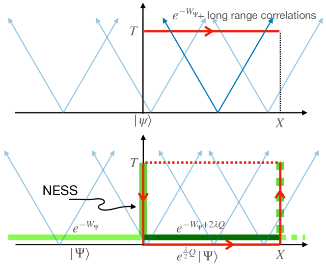
Figure 1: Illustration of the universal hydrodynamic principles for full counting statistics of the total charge $Q|_{0}^{X}(T)$ on length $X$ at time $T$ after a quench. The red contour represents this charge as an integrated density $\int_{0}^{X}{\rm d}x\,q(x,T)$ in the generator $F=\log\langle\Psi|e^{\lambda Q|_{0}^{X}(T)}|\Psi\rangle$. The contour is deformed using the continuity equation in order to avoid long-range correlations emanating from the initial state and “connecting” any parts of it (the darker blue arrows). Green bars represent steady states: from the biased quench on the right (locally $e^{\frac{\lambda}{2}Q}|\Psi\rangle$) and the original quench on the left (locally $|\Psi\rangle$), and the non-equilibrium steady state (NESS) from the partitioning protocol they induce. The specific steady state $e^{-W_{\Psi}+2\lambda Q}$ is our general result for integrable quenches. The partitioning protocols at $0$ and $X$ are independent for $X$ large enough. As every part of the deformed contour is uncorrelated, they give rise to independent contributions: the current FCS at $x=0,X$ (twice the same contribution, under parity symmetry) giving the linear growth of $F(\lambda)$ with $T$, and the charge FCS at $t=0$ giving the non-dynamical contribution.

Derivation.—  The derivation uses basic properties of many-body systems, and is illustrated in Fig. 1. From the continuity equation, $Q|_{0}^{X}(T)=\int_{0}^{X}{\rm d}x\,q(x,T)=\int_{0}^{T}{\rm d}t\,j(0,t)+\int_{0}^{X}{\rm d}x\,q(x,0)-\int_{0}^{T}{\rm d}t\,j(X,t)$, and thus in a first step:

$$\langle\Psi|e^{\lambda Q|_{0}^{X}(T)}|\Psi\rangle=\Big{(}\langle\Psi|e^{\lambda Q|_{0}^{X/2}}|\Psi\rangle\Big{)}^{2}\times$$ (10)

$$\qquad\frac{\langle\Psi|e^{\frac{\lambda}{2}Q|_{0}^{X/2}}e^{\lambda J_{0}|_{0}^{T}}e^{\frac{\lambda}{2}Q|_{0}^{X/2}}e^{\frac{\lambda}{2}Q|_{X/2}^{X}}e^{-\lambda J_{X}|_{0}^{T}}e^{\frac{\lambda}{2}Q|_{X/2}^{X}}|\Psi\rangle}{\Big{(}\langle\Psi|e^{\lambda Q|_{0}^{X/2}}|\Psi\rangle\Big{)}^{2}}$$

where $J_{x}|_{0}^{T}=\int_{0}^{T}{\rm d}t\,j(x,t)$. In the second line, we have separated exponentials as $e^{A+B}\approx e^{A}e^{B}$ by using the Baker-Campbell-Hausdorff (BCH) formula, neglecting all commutators of the operators $A_{1}=Q|_{0}^{X/2}$, $A_{2}=Q|_{X/2}^{X}$, $A_{3}=J_{0}|_{0}^{T}$ and $A_{4}=J_{X}|_{0}^{T}$. Neglecting these commutators means that the leading effects in the ballistic limit are purely classical. It is justified as follows. By locality $[A_{1},A_{2}]=O(X^{0})$ independently of time. By the Lieb-Robinson bound, or more generally, the sufficient decay of high-velocity contributions to operator evolutions, $A_{3},A_{4}$ are (with exponential accuracy) supported on regions of lengths $vT$ (for some $v$), thus in the limit $X\to\infty$ we have $[A_{1},A_{4}],\,[A_{2},A_{3}],\,[A_{3},A_{4}]\to 0$. Concerning $[A_{1},A_{3}]$ and $[A_{2},A_{4}]$, we currently do not know of general results leading to sharp bounds. However, using the fact that $Q$ is “ultra local”, we propose (see the SM) general ideas based on thinness arguments Ampelogiannis and Doyon (2023a) which support the fact that they can also be neglected, confirmed by explicit free-fermion calculations Doyon et al. (pear). The BCH formula in fact involves multiple-commutators, which can be analyzed in similar ways.

In a second step, we use results obtained by correlation matrix Bertini et al. (2024) or quench action methods Caux and Essler (2013); Caux (2016); Horváth and Rylands (2024), giving for the first factor on the right-hand side of (10)

$$\langle\Psi|e^{\lambda Q|_{0}^{X}}|\Psi\rangle\sim X(f_{W_{\Psi}}(0)-f_{W_{\Psi}}(2\lambda)).$$ (11)

This shows the term proportional to $X$ in (6). This doubling can be understood in terms of the particle-pair picture: as the free energy does not account for long-range correlations, it only encodes the distribution of single members of each pair. But in the state $e^{\frac{\lambda}{2}Q|_{0}^{X}}|\Psi\rangle$, the modified quantum amplitude gives rise to a modified probability $e^{\lambda Q|_{\rm pair}}$ for each pair, hence, at later time when members are separated, for each single member of a pair, where a doubling occur: $Q|_{\rm pair}=2Q|_{\rm single\,particle}$.

In a third step, the second factor on the right-hand side of (10) is factorised as

$$\Bigg{(}\frac{\langle\Psi|e^{\frac{\lambda}{2}Q|_{0}^{\infty}}e^{\lambda J_{0}|_{0}^{T}}e^{\frac{\lambda}{2}Q|_{0}^{\infty}}|\Psi\rangle}{\langle\Psi|e^{\lambda Q|_{0}^{\infty}}|\Psi\rangle}\Bigg{)}^{2}\quad(X\to\infty).$$ (12)

We have factorised the expectation value for operators lying far apart from each other; the extensive free-energy part in the large region $[vT,X-vT]$, centered at $X/2$, cancels in the numerator and denominator. This holds assuming appropriate clustering of the state, $|x-y|\langle\Psi|O_{1}(x)O_{2}(y)|\Psi\rangle^{c}\rightarrow 0$ as $|x-y|\rightarrow\infty$. We have then used translation invariance and parity symmetry, under which $j$ is odd and $q$ is even, to write

$$\langle\Psi|e^{\frac{\lambda}{2}Q|_{X/2}^{X}}e^{-\lambda J_{X}|_{0}^{T}}e^{\frac{\lambda}{2}Q|_{X/2}^{X}}|\Psi\rangle$$ (13)

$$=\langle\Psi|e^{\frac{\lambda}{2}Q|_{-X/2}^{0}}e^{-\lambda J_{0}|_{0}^{T}}e^{\frac{\lambda}{2}Q|_{-X/2}^{0}}|\Psi\rangle$$

$$=\langle\Psi|e^{\frac{\lambda}{2}Q|_{0}^{X/2}}e^{\lambda J_{0}|_{0}^{T}}e^{\frac{\lambda}{2}Q|_{0}^{X/2}}|\Psi\rangle.$$

The same three steps can be performed in GGEs instead of $|\Psi\rangle$. There, one can then show that the result is compatible with the expected non-equilibrium fluctuation relations Esposito et al. (2009); Bernard and Doyon (2016) (see the SM), supporting the validity of these steps.

Finally, in a fourth step, as pairs do not correlate the region $x=0,t\in[0,T]$ (see Fig.1), one may use the quench steady states locally on each region $x<0$, $x>0$ at $t=0$, using (2), (9), resp., giving the partitioning protocol (as $T\to\infty$)

$$\frac{\langle\Psi|e^{\frac{\lambda}{2}Q|_{0}^{\infty}}e^{\lambda J_{0}|_{0}^{T}}e^{\frac{\lambda}{2}Q|_{0}^{\infty}}|\Psi\rangle}{\langle\Psi|e^{\lambda Q|_{0}^{\infty}}|\Psi\rangle}\asymp\frac{{\rm Tr}\big{[}e^{\lambda J_{0}|_{0}^{T}}\,e^{-W_{\Psi}|_{-\infty}^{0}-W_{\Psi}^{\lambda}|_{0}^{\infty}}\big{]}}{{\rm Tr}\big{[}e^{-W_{\Psi}|_{-\infty}^{0}-W_{\Psi}^{\lambda}|_{0}^{\infty}}\big{]}}$$ (14)

which shows (7) with (8). Formally, this holds assuming strong enough decay of connected correlations for the current operators at different times, $|t-t^{\prime}|\langle\Psi|e^{\frac{\lambda}{2}Q|_{0}^{\infty}}j(0,t)j(0,t^{\prime})e^{\frac{\lambda}{2}Q|_{0}^{\infty}}|\Psi\rangle^{c}\rightarrow 0$ as $|t-t^{\prime}|\rightarrow\infty$.

Curved trajectories.—  The fourth step above assumes decay of correlations in time, hence no long-range correlations. There are (at least) two sources of potential long-range correlations: those arising from the inhomogeneous fluid state as shown by the BMFT Doyon et al. (2023b), and those emerging from the quench as discussed above. The former do not affect the current FCS in the partitioning protocol Doyon et al. (2023b, a). The latter, according to Fig. 1, also appear not to time-correlate the origin $x=0$.

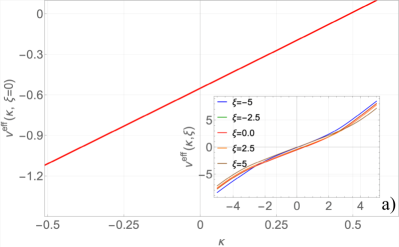
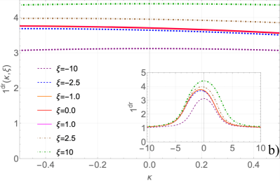
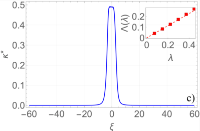
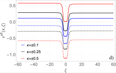
Figure S1: a) The effective velocity in the NESS ($\xi=0$) for $\kappa\in[-\Lambda,\Lambda]$ with $\Lambda\approx 0.5$, and the effective velocities for other ray-values (inset), $\xi=-5,-2.5,0,2.5,5$ corresponding to colors blue, red, black, orange and brown. b) $1^{\text{dr}}(\kappa,\xi)$ for $\kappa\in[-\Lambda,\Lambda]$ in the NESS and for further $\xi$-values, as well as at larger $\kappa$ (inset), $\xi=-10,-2.5,-1,0,1,2.5,10$ corresponding to purple (dashed), blue (dashed), orange, red, magenta, brown (dotted-dashed) and green (dotted-dashed) lines, respectively. c) The zero of $v^{\text{eff}}(\kappa^{*},\xi)$ for fixed $\xi$ as function of $\xi$ and the linear dependence of $\Lambda=\kappa^{*}(\xi=0)$ on $\lambda$ (inset). d) The effective velocity $v^{\text{eff}}(\kappa,\xi)$ as a function of $\xi$ for $\pm\kappa$ values from $[-\Lambda,\Lambda]$, where the continuous and dashed lines correspond to positive and negative rapidities, respectively, blue $\xi=0.1$, black $\xi=0.25$ and red $\xi=0.5$. The parameters are $c=1$, $d=2$ and $\lambda=0.75$.

However, the picture Fig. 1 omits the curvature of hydrodynamic trajectories in inhomogeneous fluid states. Emitted at $t=0$ are correlated pairs of fluid modes, which follow fluid characteristics in time. In interacting models, the fluid flow induced by the partitioning protocol gives rise to a “hydrodynamic waft” which curves characteristics and may make initially right-moving modes into left-moving modes (and vice versa), see Fig. 2. The impact of such curved trajectories on the evolution of entanglement in certain inhomogeneous cases have been discussed in Alba et al. (2019). For $\lambda$ small, the bias in the partitioning protocol is small, hence the effect is small. Then, only modes with small hydrodynamic velocities $\propto\lambda$ have the potential to change direction and produce long-range correlations on $x=0$, $t\in[0,T]$. In typical integrable models, there is a continuum of hydrodynamic modes Castro-Alvaredo et al. (2016); Bertini et al. (2016), parametrised by quasi-momentum $\kappa\in{\mathbb{R}}$. Modes with small hydrodynamic velocities have small quasi-momentum $|\kappa|<\Lambda\propto\lambda$ (cf. Fig. S1c in the SM) and produce small currents $\mathsf{j}\propto\kappa$. Long range correlations will only affect cumulants $c_{n}^{\lambda}$, $n\geq 2$ in the current FCS $f_{\rm dyn}=\sum_{n}c_{n}^{\lambda}\lambda^{n}/n!$, and our power-counting argument gives $c_{n}^{\lambda}\propto\mathsf{j}^{n}\propto\lambda^{n}$. As $c_{n}^{\lambda}$ occurs at order $\lambda^{n}$ in the current FCS, the lowest order where corrections may occur in $F(\lambda)$ is $\lambda^{n}\times\lambda^{n}$ for $n=2$, thus $c_{m}$ for $m\geq 4$. Further, the density of pairs produced is symmetric under $\kappa\to-\kappa$ as particles are emitted with equal and opposite momenta and by analyticity in $\kappa$, and if quasiparticles have fermionic statistics, Dirac exclusion implies vanishing at $\kappa=0$, hence a density $\sim\kappa^{2}$. This gives an additional factor $\propto\lambda^{2}$, thus, in many-body integrable models with fermionic statistics, only cumulants $c_{n}$ for $n\geq 6$ may be affected. We provide supporting calculations for this analysis in the SM.

In integrable models, formula (6) specializes to a conjecture proposed in Bertini et al. (2023, 2024), which is therefore here argued not to be generically exact for cumulants beyond order 5. In order to confirm this, using standard integrability techniques, we analyse trajectories in the above partitioning protocol corresponding to the BEC quench of the LL model, as shown in Fig. 2. At unit mass, the LL model is defined by

$$H_{\text{LL}}\!=\!\frac{1}{2}\int\!\!{\rm d}x\,b^{\dagger}(x)\!\!\left[-\partial_{x}^{2}\right]\!b(x)+2c\,b^{\dagger}(x)b(x)b^{\dagger}(x)b(x)$$ (15)

where $b^{\dagger}(x),b(x)$ are canonical spinless bosonic fields $[b(x),b^{\dagger}(y)]=\delta(x-y)$ and the BEC state takes the form

$$|\Psi\rangle_{\text{BEC}}=\lim_{N,L\rightarrow\infty}\frac{(b^{\dagger}_{0,L})^{N}}{\sqrt{N!}}|0\rangle\,,$$ (16)

where $b^{\dagger}_{0,L}$ creates a zero momentum boson in finite volume $L$ and the density $d=N/L$ is kept fixed over the limit. For finite $\lambda$, curved trajectories exist, producing long-range correlations. See the SM for details, including the clustering properties of the BEC state.

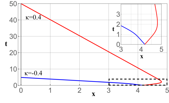
Figure 2: Illustration of curved trajectories of Euler-scale hydrodynamical modes with opposite rapidities the bi-partitioning protocol with initial density matrix $e^{-W_{\Psi}|_{-\infty}^{0}-(W_{\Psi}-2\lambda Q)|_{0}^{\infty}}$ in the LL model. The inset magnifies and better visualizes the region compassed by black dashed lines. The trajectories were constructed via the method of characteristic using the space-time dependent (effective) velocity field $v^{\text{eff}}(k,\xi=x/t,\lambda)$. The parameters are $c=1,d=2,\lambda=0.75$ and the rapidities are $\kappa=\pm 0.4$ for the right and left pairs of trajectories, respectively.

Formula (6) is expected to give all scaled cumulants $c_{n}$ in (at least) three situations. First, if the model, integrable or not, admits at most one positive, and one negative hydrodynamic velocity. Then the quench can only emit correlated pairs of fluid modes travelling in opposite directions, and for every $\lambda$ small enough, trajectories cannot be curved to produce long-range correlations on $t\in[0,T]$ at $x=0$. This includes the rule-54 model, whose FCS was shown to be given by the specialisation of (6) to this model Bertini et al. (2023, 2024). With two velocities of the same sign, one may deform the contours by slanting the “vertical branch” (c.f. Fig. 1) at a slope lying within the two velocities, again avoiding correlations: thus the formula may be generalised to this case. Second, in free particle models (or whenever the Euler hydrodynamic equation is linear): then trajectories do not curve. Finally, if the initial state is an eigenstate of $Q$: then $e^{\frac{\lambda}{2}Q}|\Psi\rangle\propto|\Psi\rangle$ and there is no partitioning, so the fluid state is uniform hence trajectories are straight.

Conclusion.—  We have derived, from general principles of many-body physics, a formula for the fluctuation of the number of particles in a gas on a large interval of size $X$, a large time $T$ after a quantum quench, in the ballistic scaling limit, with $X\gg T$. When specialised to many-body integrable systems, this formula reproduces a recent conjecture Bertini et al. (2023, 2024). We have shown how it is the physics of hydrodynamic long-range correlations that largely determine the fluctuations: the scaling with $X$ accounts for a modified thermodynamic function (evaluated exactly in integrable systems) due to such correlations produced by the quench, and its non-trivial dynamics with $T$ is solely a consequence of long-range correlations on the interval at time $T$. Crucially, our derivation shows how this dynamical effect is recast into current fluctuations at a point $x=0$ on a time interval $[0,T]$ in a special NESS. The dynamics may be modified by further long-range “waft effects” where correlated modes are transported to $x=0$ by the flow of the NESS, neglected up to now in the literature. We have argued that in integrable systems with fundamental excitations of fermionic statistics, waft effects may only, and are expected to, affect cumulants of order 6 or higher, in a way that cannot be currently evaluated. We expect that waft effects do not alter cumulants in full generality when the model admits at most two hydrodynamic velocities; and in integrable systems when hydrodynamic velocities are bounded from below in magnitude (for instance in hard rods systems). It would be interesting to extend our arguments to general $\alpha=X/T$ and other geometries, and to other charges or entanglement entropies; and to evaluate the proposed long-range effects modifying the dynamics of higher cumulants using BMFT. It would be most interesting to perform extensive numerical checks of the formula, especially in non-integrable models.

Supplementary Material - Full counting statistics after quantum quenches as hydrodynamic fluctuations

Appendix 1 Analysis of a commutator

Consider, as in the main text (with $X\to\infty$),

$$Q|_{0}^{\infty}=\int_{0}^{\infty}{\rm d}x\,q(x,0),\quad J_{0}|_{0}^{T}=\int_{0}^{T}{\rm d}t\,j(0,t).$$ (S1)

In order to underpin the arguments in the main text, we would like to show that $[Q|_{0}^{\infty},J_{0}|_{0}^{T}]$ is supported around the origin $x=0$, with a norm

$$||\,[Q|_{0}^{\infty},J_{0}|_{0}^{T}]\,||=o(T).$$ (S2)

We are not aware of general results allowing us to show this. However, a possible line of arguments is as follows.

We propose that $j(0,t)$ is composed of linear combinations of “local enough” operators supported on $x\in[-vt,vt]$ (for appropriate $v$), which become “thinner” as $t$ increases, in the sense that they become closer to the identity operator (see Ampelogiannis and Doyon (2023b)). In order to make this slightly more accurate, consider the projectors $\mathbb{P}_{x>0}$, $\mathbb{P}_{x<0}$ on operators supported on the right and left half of space (see e.g. Ampelogiannis and Doyon (2023b) for definitions of such projectors). We then propose two loosely-stated principles concerning the operator $(1-\mathbb{P}_{x>0}-\mathbb{P}_{x<0})j(0,t)$: (i) it is supported around the origin $x=0$, and (ii) it becomes closer to the identity as $t$ increases. As a consequence,

$$B(t)=[Q|_{0}^{\infty},(1-\mathbb{P}_{x>0}-\mathbb{P}_{x<0})j(0,t)]$$ (S3)

is supported around the origin, and $\int_{0}^{T}{\rm d}t\,B(t)=o(T)$ (in an appropriate norm). This is sufficient to obtain the desired result:

$$[Q|_{0}^{\infty},j(0,t)] = B(t)+[Q|_{0}^{\infty},\mathbb{P}_{x>0}j(0,t)]+[Q|_{0}^{\infty},\mathbb{P}_{x<0}j(0,t)]$$ (S4)

$$= B(t)+[Q|_{0}^{\infty},\mathbb{P}_{x>0}j(0,t)]$$ (S5)

$$= B(t)+[Q,\mathbb{P}_{x>0}j(0,t)]$$ (S6)

$$= B(t)+\mathbb{P}_{x>0}[Q,j(0,t)]$$ (S7)

$$= B(t)$$ (S8)

where we used the fact that $Q$ is ultra-local thus commute with the projection, and that the current $j$ is invariant under the action of $Q$ (preserves the particle number), $[Q,j(0,t)]=0$.

Appendix 2 Emergence of the biased GGE via Quench Action

In the following we show that after the biased quench the steady-state value of local operators is described by a biased GGE in any interacting integrable model, that is

$$\lim_{t\rightarrow\infty}\frac{\langle\Psi|O(0,t)e^{\lambda_{i}Q_{i}}|\Psi\rangle}{\langle\Psi|e^{\lambda_{i}Q_{i}}|\Psi\rangle}=\frac{1}{Z^{2\lambda_{i}}}{\rm Tr}\left[O(0,0)e^{2\lambda_{i}Q_{i}}\rho_{\text{GGE}}\right]$$ (S9)

where $\rho_{\text{GGE}}$ is the GGE that specifies that steady-state, or on other words, where the expectation value of any local operator $O$ converges,

$$\lim_{t\rightarrow\infty}\frac{\langle\Psi|O(0,t)|\Psi\rangle}{\langle\Psi|\Psi\rangle}=\frac{1}{Z}{\rm Tr}\left[O(0,0)\rho_{\text{GGE}}\right]\,.$$ (S10)

To show Eq. (S9) we shall use the reasonings of the QA method; in fact, the derivation generally applies to arbitrary integrable models as long as the fluctuations of the integrated conserved density $Q_{i}|_{-\ell/2}^{\ell/2}$ are extensive wrt. $\ell$. For simplicity, however, let us assume only one particle species. Writing the expectation value using the eigenstates of the post-quench Hamiltonian we obtain

$$\frac{\langle\Psi|O(0,t)e^{\lambda_{i}Q_{i}}|\Psi\rangle}{\langle\Psi|e^{\lambda_{i}Q_{i}}|\Psi\rangle}=\frac{1}{\langle\Psi|e^{\lambda_{i}Q_{i}}|\Psi\rangle}\sum_{\Phi,\Phi^{\prime}}e^{-\epsilon_{\Phi}^{*}-\epsilon_{\Phi^{\prime}}}e^{i(\omega_{\Psi}-\omega_{\Psi^{\prime}})t}\langle\Phi|O(0,0)e^{\lambda_{i}Q_{i}}|\Phi^{\prime}\rangle\,,$$ (S11)

where $\epsilon_{\Phi}=-\log{\langle\Phi|\Psi\rangle}$ are the logarithmic overlaps. Following the logic of the Quench Action (QA) method Caux and Essler (2013); Caux (2016), we can replace one summation by a functional integral over root distributions assuming that the size of the entire system $L$ is very large and is eventually sent to infinity. This way we may write

$$\frac{\langle\Psi|O(0,t)e^{\lambda_{i}Q_{i}}|\Psi\rangle}{\langle\Psi|e^{\lambda_{i}Q_{i}}|\Psi\rangle}=\sum_{\Phi}\!\int\!\mathcal{D}[\rho]e^{S_{YY}[\rho]}\!\left[e^{-\epsilon_{\Phi}^{*}-\epsilon[\rho]}e^{i(\omega_{\Psi}-\omega[\rho])t}\langle\Phi|O(0,0)e^{\lambda_{i}Q_{i}}|\rho\rangle+\Phi\leftrightarrow\rho\vphantom{\frac{OOOOO}{OOOOO}}\right]\times\frac{1}{\langle\Psi|e^{\lambda_{i}Q_{i}}|\Psi\rangle},\quad\quad\quad$$ (S12)

where $S_{YY}$ is the Yang-Yang entropy of the root distribution whose exponential gives the number of microstates with the same root distribution. Note that this quantity is proportional to the system size $L$. The usual reasoning of QA comes from the recognition that when $t$ is sent to $\infty$, because of the oscillatory factor and the behaviour of matrix elements in the thermodynamic limit, the summation over the eigenstates $\Phi$ can be terminated and replaced by a single eigenstate that corresponds to the macro-state $\rho$, i.e.,

$$\frac{\langle\Psi|O(0,\infty)e^{\lambda_{i}Q_{i}}|\Psi\rangle}{\langle\Psi|e^{\lambda_{i}Q_{i}}|\Psi\rangle}=\int\mathcal{D}[\rho]O[\rho]e^{S_{YY}[\rho]-2\text{Re}\,\epsilon[\rho]+L\int\text{d}k\,\lambda_{i}q_{i}(k)\rho(k)}\times\left[\int\mathcal{D}[\rho]e^{S_{YY}[\rho]-2\text{Re}\,\epsilon[\rho]+L\int\text{d}k\,\lambda_{i}q_{i}(k)\rho(k)}\right]^{-1}\,,$$ (S13)

where we also exploited the fact the $Q_{i}$ is an extensive conserved quantity and hence can be naturally rewritten in terms of the root-distributions. In the thermodynamic limit, the functional integral over the root densities can be replaced by its saddle-point value, since not only the Yang-Yang entropy, but also the conserved charge and by definition, the extensive part of the logarithmic overlap $\epsilon[\rho]$ scale with the system size $L$. The main ingredient which we further utilize is that a local operator cannot shift the saddle point, which, accordingly, is determined by the denominator. In the usual fashion of QA, we can write the exponential in denominator as

$$-L\int_{0}^{\infty}\text{d}k\,g(k)\rho(k)+L\int_{-\infty}^{\infty}\text{d}k\,\lambda_{i}q_{i}(k)\rho(k)-L\int_{0}^{\infty}\text{d}k\,s_{YY}[\rho(k)]\,,$$ (S14)

where $s_{YY}$ is the Yang-Yang entropy density and for integrable quenches,

$$-2\text{Re}\,\epsilon[\rho]=L\int_{0}^{\infty}{\rm d}k\,g(k)\rho(k)\,.$$ (S15)

Note that the lower limit for the spectral integration is zero for the YY entropy and for the overlap contribution; this is due the distinctive feature of integrable quenches that the corresponding initial states in the post quench basis consists solely of pairs of excitation with opposite momentum. Exploiting translation invariance $\rho$ can be regarded as an even function and we can rewrite the integrals as

$$-\frac{L}{2}\int_{-\infty}^{\infty}\text{d}k\,g(k)\rho(k)+\frac{L}{2}\int_{-\infty}^{\infty}\text{d}k\,2\lambda_{i}q_{i}(k)\rho(k)-\frac{L}{2}\int_{-\infty}^{\infty}\text{d}k\,s_{YY}[\rho(k)]\,,$$ (S16)

from which the saddle-point equations are obtained via functional differentiation wrt. $\rho$ yielding

$$0=g(k)-2\lambda_{i}q_{i}(k)+\frac{\delta s_{YY}[\rho]}{\delta\rho(k)}\,,$$ (S17)

which can be recast in the conventional TBA form for the saddle-point density $\rho_{\text{sp}}$ via the pseudo-energy $\epsilon$ as

$$\epsilon(k)=g(k)-2\lambda_{i}q_{i}(k)-\varphi\star\log\left(1+e^{-\epsilon}\right)\,.$$ (S18)

The equation above characterises a GGE via the spectral densities $\epsilon$ and $\rho_{\text{sp}}$ which can be computed from the former. Indeed, it has been shown that

$$g(k)=-\sum\beta_{i}q_{i}(k)$$ (S19)

for free fermion quenches Calabrese et al. (2012b) and for the Lieb-Liniger model and the BEC quench De Nardis et al. (2014); Pálmai and Konik (2018). That is, the driving term $g(k)-2\lambda_{i}q_{i}(k)$ must correspond to a GGE with charge $Q_{i}$ biased by $2\lambda_{i}$. Since, as already mentioned, local operators do not shift the saddle-point of the QA functional Pozsgay (2011), the steady-state expectation value of $O$ is determined by $\rho_{\text{sp}}^{2\lambda_{i}}$ where we made it explicit that $\rho_{\text{sp}}^{2\lambda_{i}}$ is associated with the solution of Eq. (S18) and accordingly,

$$\lim_{t\rightarrow\infty}\lim_{L\rightarrow\infty}\frac{\langle\Psi|O(0,t)e^{\lambda_{i}Q_{i}}|\Psi\rangle}{\langle\Psi|e^{\lambda_{i}Q_{i}}|\Psi\rangle}=\int{\rm d}k\,O[\rho_{\text{sp}}(k)]=\frac{1}{Z^{2\lambda_{i}}}{\rm Tr}\left[O(0,0)e^{2\lambda_{i}Q_{i}}\rho_{\text{GGE}}\right]\,,$$ (S20)

where $\rho_{\text{GGE}}$ is the GGE dictated by integrable quench, i.e., the unmodified integrable initial state $|\Psi\rangle$. It is also immediate to see that using the same reasoning for the nominator

$$\lim_{t\rightarrow\infty}\lim_{L\rightarrow\infty}\frac{\langle\Psi|e^{\lambda_{i}/2Q_{i}}O(0,t)e^{\lambda_{i}/2Q_{i}}|\Psi\rangle}{\langle\Psi|e^{\lambda_{i}Q_{i}}|\Psi\rangle}=\int{\rm d}k\,O[\rho_{\text{sp}}(k)]=\frac{1}{Z^{2\lambda_{i}}}{\rm Tr}\left[O(0,0)e^{2\lambda_{i}Q_{i}}\rho_{\text{GGE}}\right]\,,$$ (S21)

holds as well, as expected.

Appendix 3 Implications of the hydrodynamic fluctuation relations

In this subsection we demonstrate that the hydrodynamic fluctuation relations Esposito et al. (2009); Bernard and Doyon (2016) which were derived for thermal states strongly confirms the validity of performing steps such as $e^{A+B}\approx e^{A}a^{B}$ for the eventual quench problem in the LL model and consequently in a broad class of interacting integrable systems as well. More precisely, we show that fluctuation relations are compatible with writing (10) in thermal or GGE ensembles indirectly justifying the legitimacy of such steps in GGEs from which we infer the validity of (10) for the quench problem as well.

The main idea is to consider the FCS in a thermal ensemble and exploit its time-independence. In particular using the contour deformation from the main text we may write $F(\lambda_{i},X,T)=Tf_{\text{dyn}}^{\text{L}}(\lambda_{i})+Tf_{\text{dyn}}^{\text{R}}(\lambda_{i})+Xf^{0}(\lambda_{i})$ with $X\gg T\gg 1$ up to sub-leading corrections as in the main text, with

$$\begin{split}f_{\text{dyn}}^{\text{L}}(\lambda_{i})=&\lim_{T\rightarrow\infty}T^{-1}\lim_{X\rightarrow\infty}\frac{\ln{\rm Tr}[e^{\lambda J_{0}|_{0}^{T}+\lambda Q|_{0}^{X/2}(0)}\rho_{\text{GGE}}]}{\ln{\rm Tr}[e^{\lambda Q|_{0}^{X/2}(0)}\rho_{\text{GGE}}]}\\ f_{\text{dyn}}^{\text{R}}(\lambda_{i})=&\lim_{T\rightarrow\infty}T^{-1}\lim_{X\rightarrow\infty}\frac{\ln{\rm Tr}[e^{\lambda Q|_{X/2}^{X}(0)-\lambda J_{X}|_{0}^{T}}\rho_{\text{GGE}}]}{\ln{\rm Tr}[e^{\lambda Q|_{X/2}^{X}(0)}\rho_{\text{GGE}}]}\,,\end{split}$$ (S22)

where we may recall the cluster property of GGEs. $f^{0}(\lambda_{i})$ is the SCGF in a GGE, which must be equal to $\lim_{x\rightarrow\infty}F(\lambda_{i},T,X)/X$ due to the stationary property of GGEs implying that

$$\lim_{X\rightarrow\infty}\frac{\ln{\rm Tr}[e^{\lambda J_{0}|_{0}^{T}+\lambda Q|_{0}^{X/2}(0)}\rho_{\text{GGE}}]}{\ln{\rm Tr}[e^{\lambda Q|_{0}^{X/2}(0)}\rho_{\text{GGE}}]}+\lim_{X\rightarrow\infty}\frac{\ln{\rm Tr}[e^{\lambda Q|_{X/2}^{X}(0)-\lambda J_{X}|_{0}^{T}}\rho_{\text{GGE}}]}{\ln{\rm Tr}[e^{\lambda Q|_{X/2}^{X}(0)}\rho_{\text{GGE}}]}=0$$ (S23)

must hold. Rewriting $f_{\text{dyn}}^{\text{L}}(\lambda_{i})$ as

$$f_{\text{dyn}}^{\text{L}}(\lambda_{i})=\lim_{T\rightarrow\infty}T^{-1}\frac{\ln{\rm Tr}[e^{\lambda J_{0}|_{0}^{T}}e^{\lambda Q|_{0}^{\infty}(0)}\rho_{\text{GGE}}]}{\ln{\rm Tr}[e^{\lambda Q|_{0}^{\infty}(0)}\rho_{\text{GGE}}]}\,,$$ (S24)

it also follows that

$$f_{\text{dyn}}^{\text{L}}(\lambda_{i})+f_{\text{dyn}}^{\text{R}}(\lambda_{i})=0\,.$$ (S25)

The important recognition is that, by definition, the quantity $f_{\text{dyn}}^{\text{L}}(\lambda_{i})$ equals the SCGF of the $i$th current, in a NESS after a bi-partite quench where the left semi-infinite system is characterised by a GGE, $\rho_{\text{GGE}}$; and the right half is by $e^{\lambda_{i}Q_{i}}\rho_{\text{GGE}}$. Importantly, unlike in the quench problem, $e^{\lambda_{i}Q_{i}}\rho_{\text{GGE}}$, is a biased GGE where $\beta_{i}$ becomes shifted to $\beta_{i}-\lambda_{i}$ (and not $2\lambda_{i}$), by definition. We have assumed that the system locally equilibrates to the NESS of this bi-partitioning protocol as well as the lack of strong temporal long-range correlations in NESS, which is legitimate since in GGEs quasi-particles with opposite momentum are not correlated. In other words, we have found that

$$f_{\text{dyn}}^{\text{L}}(\lambda_{i})=f^{\text{bpp}}(\lambda_{i})\,,$$ (S26)

where $f^{\text{bpp}}(\lambda_{i})$ is the SCGF if the $i$th current in the NESS of the GGE emerging after the aforementioned partitioning protocol and which has been studied in the literature Esposito et al. (2009); Bernard and Doyon (2016). In particular $f^{\text{bpp}}(\lambda_{i})$ satisfies the hydrodynamic fluctuation relations, i.e.,

$$f^{\text{bpp}}(\lambda_{i})=f^{\text{bpp}}(\beta_{i}^{\text{R}}-\beta_{i}^{\text{L}}-\lambda_{i})$$ (S27)

and since in our case $\beta_{i}^{\text{L}}=\beta_{i}$ and $\beta_{i}^{\text{R}}=\beta_{i}-\lambda_{i}$, we find that

$$f^{\text{bpp}}(\lambda_{i})=f^{\text{bpp}}(0)=0$$ (S28)

guaranteeing (S23), even term by term, at least for large T. In other words we have shown that the hydrodynamic fluctuation relations imply the expected invariance of the charge FCS in GGEs if the step (10) is performed and no strong temporal correlations affecting current fluctuations are assumed. That is, the fulfillment of these assumptions in GGEs is consistent with physical requirements, such as the implication of hydrodynamic fluctuation relations or the invariance of GGEs. These findings make performing (10) for the quench problem very plausible.

Appendix 4 The hydrodynamic flow equations for $f_{\text{dyn}}(\lambda_{i})$ in integrable models

4.0.1 Describing macro-states in integrable models

Integrable models admit an extensive number of (quasi-) local commuting conserved quantities charges $Q_{l},~{}l=1,2,\dots$ including the Hamiltonian. Consequently such models have a stable set of quasi-particle excitations which are indexed by a discrete species index $n=1,\dots,N_{s}$ and parameterized by a continuous rapidity $k^{(n)}_{j}$, $j=1,\dots,M_{n}$, but simplicity, we restrict our discussion to models with only one species. An eigenstate of the model is specified by the rapidities of quasi-particles, and is denoted by $|\bm{k}\rangle=|k_{1},\ldots,k_{M}\rangle$. These states are simultaneous eigenstates of all the conserved charges, namely $Q_{l}|\bm{k}\rangle=\sum_{j=1}^{M}q_{l}(k_{j})|\bm{k}\rangle$. Conserved charges can be categorized as even or odd ones wrt. spatial parity such as the particle number $N=Q_{0}$ or the Hamiltonian $H=Q_{2}$; and the total momentum $P=Q_{1}$, respectively. For simplicity we denote the charge, momentum and energy of a quasi-particle of rapidity $k$ by $q=q_{0}(k),p(k)=q_{1}(k)$ and $E(k)=q_{2}(k)$. In the thermodynamic limit and at finite (particle, energy, etc) density the model can be treated using the methods of the thermodynamics Bethe Ansatz (TBA) Takahashi (1999). Such states are described through distributions related to their quasi-particle content, in particular, $\rho(k),\rho^{h}(k),\rho^{t}(k)$ and $\theta(k)$ which are respectively the distribution of occupied, the distribution unoccupied quasiparticles, the total density of states $\rho^{t}(k)=\rho(k)+\rho^{h}(k)$ and the occupation function $\theta(k)=\rho(k)/\rho^{t}(k)$. These functions are related to each other by the Bethe-Takahashi equations

$$\rho^{t}(k)=\frac{p^{\prime}(k)}{2\pi}+\varphi\star\rho(k)$$ (S29)

where $(\cdot)^{\prime}$ denotes differentiation w.r.t. $k$ and $\star$ is the convolution $f\star g(x)=\int\frac{{\rm d}y}{2\pi}f(x-y)g(y)$. $\varphi(k-k^{\prime})$ is the scattering kernel which characterizes the scattering between quasi-particles with rapidities $k$ and $k^{\prime}$.

When macro-state are considered containing many excitations the bare quasi-particle properties become dressed due to the interactions. Dressed quantities denoted by $(\cdot)^{\rm dr}$ satisfy the integral equation

$$f^{\rm dr}(k)=f(k)+\varphi\star[\theta(k)f^{\rm dr}(k)].$$ (S30)

A particularly important quantity is the effective velocity of the quasi-particles given by the ratio of dressed quantities, $v^{\text{eff}}(k)={E^{\prime}}^{\rm dr}(k)/{p^{\prime}}^{\rm dr}(k)$.

To better expose the flow equations for $f_{\text{dyn}}(\lambda_{i})$ we specified an important quantum model, the Lieb–Liniger model defined by

$$H_{\text{LL}}\!=\!\frac{1}{2}\int\!\!{\rm d}x\,b^{\dagger}(x)\!\!\left[-\frac{\partial_{x}^{2}}{m}\right]\!b(x)+2c\,b^{\dagger}(x)b(x)b^{\dagger}(x)b(x).$$ (S31)

where we set $m=1$ and $b^{\dagger}(x),b(x)$ are canonical spinless bosonic operators satisfying $[b(x),b^{\dagger}(y)]=\delta(x-y)$. The Hamiltonian (S31) describes bosons of mass $m$ interacting via a density-density interaction of strength $c>0$ corresponding to repulsion between the bosons. For the out-of-equilibrium dynamics ceratain integrable quenches are considered Piroli et al. (2017). Via the Quench Action method Caux and Essler (2013); Caux (2016), it is possible to characterize the steady-state GGE for such quenches. These quenches also have the distinctive property that the initial states have non-vanishing overlaps with the eigenstates of the post-quench Hamiltonian only if these states consist of pairs of particles with opposite momentum/rapidity. For the LL model we consider the Bose-Einstein condensate states as such integrable initial state (BEC) defined as

$$|\Psi\rangle_{\text{BEC}}=\lim_{N,L\rightarrow\infty}\frac{(b^{\dagger}_{0,L})^{N}}{\sqrt{N!}}|0\rangle\,,$$ (S32)

respectively, where $b^{\dagger}_{0,L}$ creates a zero momentum boson in finite volume $L$ and when taking the thermodynamic limit the density $N/L=d$ is kept fixed and the state is also the ground state of the LL model at $c=0$.

For these initial states it possible to compute the the steady-state spectral densities corresponding to the GGE via solving

$$\ln\eta(k)=g(k)-\left(\varphi\star\ln[1+\eta^{-1}]\right)(k)$$ (S33)

where $\varphi(k)=\frac{2|c|}{c^{2}+k^{2}}$ with $g=\ln[k^{2}(k^{2}+(c/2)^{2})]-2\ln[d\,c]$, and where $\theta(k)=1/(1+\eta(k))$. De Nardis et al. (2014).

4.0.2 Hydrodynamic predictions for FCS and SCGF

In the following we specify the results for the FCS which have been first obtained in Bertini et al. (2023, 2024) via space-time swap, and in this Letter using hydrodynamic principles. The validity of these principles in the particularly important case of free models will be presented elsewhere Doyon et al. (pear). In particular, applying the description of integrable systems, the predictions of (6) for the function $f_{\text{dyn}}(\lambda_{i})$ can be further specified as follows. We write $2f_{\text{dyn}}(\lambda_{i})=f_{\text{j}_{\text{L}}}^{\rho_{\text{L}}}(\lambda_{i})+f_{\text{j}_{\text{R}}}^{\rho_{\text{R}}}(\lambda_{i})$, which are associated with the fluctuations of the corresponding current along the left (L) and right (R) regions, c.f. Fig. 1. Using the shorthand y=L,R (6) dictates that $f_{\text{j}_{y}}^{\rho_{\text{y}}}$ are defined through the flow equations

$$f_{\text{j}_{y}}^{\rho_{\text{y}}}(\lambda_{i})=\int_{0}^{\pm\lambda_{i}}\!\!\!\!\!{\rm d}\beta_{i}\!\!\int\frac{{\rm d}k}{2\pi}E^{\prime}(k)\tilde{\theta}_{\text{y}}^{\beta_{i}}(k)q^{\text{dr}}_{i}[\tilde{\theta}_{\text{y}}^{\beta_{i}}](k)\,,$$ (S34)

with the quantities in the integrand satisfying

$$\begin{split}&\partial_{\beta_{i}}\epsilon^{\beta_{i}}_{\text{y}}(k)=-\text{sgn}(v^{\text{eff}}[\tilde{\theta}_{\text{y}}^{\beta_{i}}](k))q^{\text{dr}}_{i}[\tilde{\theta}_{\text{y}}^{\beta_{i}}](k)\\ &\tilde{\theta}_{\text{y}}^{\beta_{i}}(k)=\frac{1}{\exp[\epsilon^{\beta_{i}}_{\text{y}}(k)]+1},\quad\text{with}\quad\tilde{\theta}^{0}_{\text{y}}(k)=\theta_{\text{y}}(k)\,.\end{split}$$ (S35)

The initial condition is specified by the NESS ($x\ll t$) of a bi-partitioning protocol as

$$\begin{split}\theta_{\text{L}}(k)&=\Theta_{\text{H}}(v^{\text{eff}}(k))\theta(k)+\Theta_{\text{H}}(-v^{\text{eff}}(k))\theta^{(\lambda_{i})}(k)\\ \theta_{\text{R}}(k)&=\Theta_{\text{H}}(v^{\text{eff}}(k))\theta^{(\lambda_{i})}(k)+\Theta_{\text{H}}(-v^{\text{eff}}(k))\theta(k)\,,\end{split}$$ (S36)

where $\Theta_{\text{H}}$ is the Heaviside-theta function and the filling function $\theta(k)$ correspond to the GGE $\rho_{\text{GGE}}$ and $\theta^{(\lambda_{i})}(k)$ to a modified GGE defined by the steady state for $\langle\Psi|O(t,x)e^{\lambda_{i}Q_{i}}|\Psi\rangle$ at late times. For integrable initial states, $\theta^{(\lambda_{i})}(k)$ is obtained from Eq. (S33) upon replacing $g(k)$ by $g(k)-2\lambda_{i}q_{i}(k)$ corresponding to $\rho_{\text{GGE}}e^{2\lambda_{i}Q_{i}}$.

4.1 Clustering of the BEC state

We can comment on the clustering properties of the BEC state, $|\Psi\rangle_{\text{BEC}}$. Indeed this state has very mundane, yet not always trivial correlations. In particular it is easy to check that

$$\begin{split}\phantom{o}{}_{\text{BEC}}\langle\Psi|b^{\dagger}(x)b(y)|\Psi\rangle^{c}_{\text{BEC}}=&\lim_{L,N\rightarrow\infty}\frac{1}{L}\sum_{k,p}\langle 0|\frac{(b_{0,L})^{N}}{\sqrt{N!}}b_{k,L}^{\dagger}b_{k^{\prime},L}\frac{(b_{0,L}^{\dagger})^{N}}{\sqrt{N!}}|0\rangle e^{{\rm i}(k^{\prime}y-kx)}\\ =&\lim_{L,N\rightarrow\infty}\frac{1}{L}\langle 0|\frac{(b_{0,L})^{N}}{\sqrt{N!}}b_{0,L}^{\dagger}b_{0,L}\frac{(b_{0,L}^{\dagger})^{N}}{\sqrt{N!}}|0\rangle=\lim_{L,N\rightarrow\infty}\frac{N}{L}=d\,.\end{split}$$ (S37)

using that in finite volume $b(x)=\frac{1}{\sqrt{L}}\sum_{k}e^{ikx}b_{k,L}$, that is, certain correlations do not decay. However 2pt connected correlation functions of operators of the form $(b^{\dagger}(x))^{n}(b(x))^{n}$ (including possible derivatives as well) such as the particle density ($n=1$) do satisfy the cluster property. For our cases of interest it is sufficient to focus on this class of operators since they do not change particle number which is also conserved by the dynamics. For the particular case of the density operator, we can write

$$\begin{split}\phantom{o}{}_{\text{BEC}}\langle\Psi|b^{\dagger}(x)b(x)b^{\dagger}(y)b(y)|\Psi\rangle_{\text{BEC}}=&\lim_{L,N\rightarrow\infty}\frac{1}{L^{2}}\sum_{k,k^{\prime},p,p^{\prime}}\langle 0|\frac{(b_{0,L})^{N}}{\sqrt{N!}}b_{k,L}^{\dagger}b_{k^{\prime},L}b_{p,L}^{\dagger}b_{p^{\prime},L}\frac{(b_{0,L}^{\dagger})^{N}}{\sqrt{N!}}|0\rangle e^{{\rm i}(k^{\prime}-k)x}e^{{\rm i}(p^{\prime}-p)y}\\ =&\lim_{L,N\rightarrow\infty}\frac{1}{L^{2}}\sum_{p}\langle 0|\frac{(b_{0,L})^{N}}{\sqrt{N!}}b_{0,L}^{\dagger}b_{p,L}b_{p,L}^{\dagger}b_{0,L}\frac{(b_{0,L}^{\dagger})^{N}}{\sqrt{N!}}|0\rangle e^{{\rm i}p(x-y)}\\ &=d^{2}+\lim_{L,N\rightarrow\infty}\frac{1}{L^{2}}\sum_{p\neq 0}\langle 0|\frac{(b_{0,L})^{N}}{\sqrt{N!}}b_{0,L}^{\dagger}b_{0,L}\frac{(b_{0,L}^{\dagger})^{N}}{\sqrt{N!}}|0\rangle e^{{\rm i}p(x-y)}\\ &=d^{2}+\lim_{L,N\rightarrow\infty}\frac{N}{L^{2}}\sum_{p}e^{{\rm i}p(x-y)}-\frac{N}{L^{2}}=d^{2}+d\delta(x-y)\,,\end{split}$$ (S38)

that is,

$$\phantom{o}{}_{\text{BEC}}\langle\Psi|q(x)q(y)|\Psi\rangle^{c}_{\text{BEC}}=d\delta(x-y).$$ (S39)

For correlation functions of $(b^{\dagger}(x))^{n}(b(x))^{n}$ operators analogous calculations predict $d^{n}\delta^{n}(x-y)$ behaviors. The higher powers of the Dirac-$\delta$ function can be regularized by point splitting, which results in $\delta$-correlated connected 2pt functions.

4.2 Curved trajectories of hydrodynamical modes and dynamical long-range correlations in interacting models

One main finding of this letter is that curved hydrodynamic trajectories together with spatial short-range initial correlation and certain initial correlations in momentum or rapidity space give rise to long-range correlations for the time integrated current, hence the predictions of BFT for the initial time evolution of the scaled cumulants of conserved charges are not correct. More precisely, the connected correlation function

$$\frac{\langle\Psi|e^{\lambda/2\,Q|_{0}^{\infty}(0)}j(0,t)j(0,t^{\prime})e^{\lambda/2\,Q|_{0}^{\infty}(0)}|\Psi\rangle^{c}}{\langle\Psi|e^{\lambda Q|_{0}^{\infty}(0)}|\Psi\rangle}$$ (S40)

at finite counting field, as well as higher point connected correlation functions exhibit slow decay upon separating the time arguments of the currents, which prevent the applicability of BFT to compute the SCGF of the current after the bipartite quench from $e^{\lambda/2\,Q|_{0}^{\infty}(0)}|\Psi\rangle$, which translates into the time evolution of the SCGF of the corresponding integrated conserved charge.

In the following we demonstrate the validity of the above claim via the example of the LL model and the BEC quench using a series of non-trivial arguments. Therein, a particularly important role is played by the BMFT whose main assumption is that spatio-temporal fluctuations, and hence also correlations can be described by considering the fluctuations in the initial state and appropriately transporting them via the Euler hydrodynamic equations of the conserved quantities in integrable systems admitting ballistic transport.

The other cornerstone regards the correlations in the initial state. In particular, since in the post-quench expansion of integrable initial state excitations with opposite momentum or rapidity are correlated we expect certain correlations for rapidity-resolved conserved quantities or hydrodynamical normal modes. While the intuition for this claim is natural, the characterization of such correlations via rapidity-resolved conserved quantities in genuinely interacting integrable models is non-trivial.

Regarding the construction of rapidity-resolved conserved quantities in interacting integrable models, this task has been achieved in Ilievski et al. (2016, 2017); Doyon and Hübner (2023). However, for our purposes and to apply the BMFT equations, the (semi-)locality properties of such charges are an important ingredient, which have only partially been studied and verified in Ilievski et al. (2017); Doyon and Hübner (2023). On the contrary, the construction of rapidity-resolved conserved quantities is particularly simple in free fermion models and their semi-locality properties are also well-established del Vecchio del Vecchio et al. (2024b).

In the following, therefore, we shall refer to free fermion quenches which is also motivated by one more technical reason. Whereas computing the rapidity-resolved correlations of conserved charges after the BEC quench is possible, at least in principle, the computation would require a linked-cluster expansion with a three-fold summation over LL eigenstates using exact overlap formulas and the form factors of the the model, and hence might not be practically feasible. To avoid such technicalities we rather consider the rapidity-resolved correlation functions in the free fermion model after free fermion integrable quenches, exploiting the key structural similarity of integrable quenches, i.e., consisting of pairs of excitations with opposite momentum. In other words, we shall infer the input for the BMFT equations for the LL model by first studying the correlation functions of rapidity resolved conserved charges in the free fermion model.

4.2.1 Rapidity-resolved conserved quantities

As we have mentioned there are known constructions for rapidity-resolved conserved charges in interacting integrable models, however, for various reasons we shall consider the corresponding charges in the free-fermion model, where the construction is particularly straightforward del Vecchio del Vecchio et al. (2024b). Using the standard Fourier decomposition of the fermion field operators,

$$\psi(x,t)=\frac{1}{\sqrt{2\pi}}\int{\rm d}k\,e^{{\rm i}kx-{\rm i}E_{k}t}a_{k}\,,\quad\psi^{\dagger}(x,t)=\frac{1}{\sqrt{2\pi}}\int{\rm d}k\,e^{-{\rm i}kx+{\rm i}E_{k}t}a^{\dagger}_{k}\,,$$ (S41)

and

$$a_{k}=\frac{1}{\sqrt{2\pi}}\int\text{d}ke^{-{\rm i}kx}\psi(x)\,,\quad a^{\dagger}_{k}=\frac{1}{\sqrt{2\pi}}\int\text{d}ke^{{\rm i}kx}\psi^{\dagger}(x)$$ (S42)

with basic anti-commutators

$$\{\psi^{\dagger}(x),\psi(y)\}=\delta(x-y),\quad\{a_{k}^{\dagger},a_{p}\}=\delta(k-p).$$ (S43)

where we can write a conserved charge of the particle number as del Vecchio del Vecchio et al. (2024b)

$$Q=\sum_{\kappa_{n}}Q_{\kappa_{n}}\,,\text{ with }\quad Q_{\kappa_{n}}=\int_{\kappa_{n}-\epsilon/2}^{\kappa_{n}+\epsilon/2}\!\!\!\!\!{\rm d}k\,a^{\dagger}_{k}a_{k}$$ (S44)

where $\kappa_{n}=n\epsilon$. The rapidity-resolved particle density can be written as well del Vecchio del Vecchio et al. (2024b) as

$$q(x,t)=\sum_{\kappa_{n}}q_{\kappa_{n}}(x,t)\,,\text{ with }\quad q_{\kappa_{n}}(x,t)=\frac{1}{2\pi}\int_{-\infty}^{\infty}\!\!\!{\rm d}k\,{\rm d}k^{\prime}\,e^{-{\rm i}(k-k^{\prime})x}e^{{\rm i}(E_{k}-E_{k^{\prime}})t}\Theta_{\text{H}}(\epsilon/2-|k+k^{\prime}-2\kappa_{n}|/2)a^{\dagger}_{k}a_{k^{\prime}}\,,$$ (S45)

where $\Theta_{\text{H}}$ is the Heaviside Theta function and more explicitly

$$\Theta_{\text{H}}(\epsilon/2-|k+k^{\prime}-2\kappa_{n}|/2)=\Theta_{\text{H}}(\epsilon/2-(k+k^{\prime})/2+\kappa_{n})-\Theta_{\text{H}}(-\epsilon/2-(k+k^{\prime})/2+\kappa_{n})\,.$$ (S46)

4.2.2 Rapidity-resolved spatial correlations in the fermionic initial states

As we have outlined before, a crucial ingredient to evaluate dynamical long-range correlations in the LL model, is the knowledge of the rapidity-resolved spatial correlation of the particle number operator at the initial state. More precisely, however, these initial correlations must be regarded already at the Euler scale, due the requirements of BMFT, that is, we are interested in the quantity

$$\lim_{t\rightarrow 0}\lim_{\ell\rightarrow\infty}\ell\times_{\text{BEC}}\!\langle\Psi|q_{\kappa_{n}}(\ell x,\ell t)q_{\kappa_{n^{\prime}}}(\ell x^{\prime},\ell t)|\Psi\rangle^{c}_{\text{BEC}}\neq\lim_{\ell\rightarrow\infty}\ell\times_{\text{BEC}}\!\langle\Psi|q_{\kappa_{n}}(\ell x,0)q_{\kappa_{n^{\prime}}}(\ell x^{\prime},0)|\Psi\rangle^{c}_{\text{BEC}}\,.$$ (S47)

The computation of this object for the LL model is notoriously complicated and, in principle, might be carried out using a non-trivial and tedious form factor expansion. For this reason we rather compute the corresponding 2pt function in fermionic initial states and will use the result as initial input for the BMFT equations for the interacting case. This approximation is justified by the universal structure of integrable initial states, namely the existence of correlated pairs of excitations with opposite momentum. Therefore, we first consider

$$\lim_{t\rightarrow 0}\lim_{\ell\rightarrow\infty}\ell\times_{\text{FF}}\!\langle\Psi|q_{\kappa_{n}}(\ell x,\ell t)q_{\kappa_{n^{\prime}}}(\ell x^{\prime},\ell t)|\Psi\rangle^{c}_{\text{FF}}\,,$$ (S48)

where $|\Psi\rangle_{\text{FF}}$ is characterized by a K-function $K(k)$ or by $K(k)e^{2\lambda}$ as

$$|\Psi\rangle_{\text{FF}}=\mathcal{N}_{\text{FF}}^{-1/2}\left(\exp{\int_{0}^{\infty}\frac{{\rm d}k}{2\pi}K(k)a^{\dagger}_{k}a^{\dagger}_{-k}}\right)|0\rangle\,.$$ (S49)

Importantly, the free fermion quench problem can be analyzed exploiting the Bogolyubov transformation

$$a_{p}=u_{p}\tilde{a}_{p}+v_{p}\tilde{a}^{\dagger}_{-p}\,,\qquad a^{\dagger}_{p}=v^{*}_{p}\tilde{a}_{-p}+u_{p}\tilde{a}^{\dagger}_{p}\,\quad\text{where}\quad u_{p}=\frac{1}{\sqrt{1+|K(p)|^{2}}}\,,\,v_{p}=\frac{K(p)}{\sqrt{1+|K(p)|^{2}}}\,$$ (S50)

with the new fermion operators $\tilde{a}_{p}$ annihilating $|\Psi\rangle_{\text{FF}}$. Using this transformation, the 2pt density correlation function is easy to express Doyon et al. (pear) from which, using del Vecchio del Vecchio et al. (2024b), we obtain the momentum-resolved correlation function as

$$\begin{split}&\phantom{}{}_{\text{FF}}\langle\Psi|q_{\kappa_{n}}(\ell x,\ell t)q_{\kappa_{n^{\prime}}}(\ell x^{\prime},\ell t)|\Psi\rangle^{c}_{\text{FF}}=\\ &=\int\frac{{\rm d}k}{2\pi}\frac{{\rm d}p}{2\pi}\left\{\frac{|K(k)|^{2}}{1+|K(k)|^{2}}\frac{1}{1+|K(p)|^{2}}e^{-{\rm i}(k-p)(x-x^{\prime})}e^{{\rm i}t(E_{k}-E_{p})}\Theta_{\text{H}}(\epsilon/2-|k+p-2\kappa_{n}|/2)\Theta_{\text{H}}(\epsilon/2-|k+p-2\kappa_{n}^{\prime}|/2)\right.\\ &\left.\qquad\qquad+\frac{K^{*}(k)}{1+|K(k)|^{2}}\frac{K(p)}{1+|K(p)|^{2}}e^{-{\rm i}(k-p)(x-x^{\prime})}e^{{\rm i}t(E_{k}-E_{p})}\Theta_{\text{H}}(\epsilon/2-|k+p-2\kappa_{n}|/2)\Theta_{\text{H}}(\epsilon/2-|k+p+2\kappa_{n}^{\prime}|/2)\right\}\,.\end{split}$$ (S51)

In the following we show that the last line gives rise to $\delta(\kappa+\kappa^{\prime})$ type correlations when $\epsilon\rightarrow 0$ (whereas the first line corresponds to $\delta(\kappa-\kappa^{\prime})$) hence we restrict our attention to the last line of (S51). To proceed, we approximate the box-function originating from the Heaviside Theta function (c.f. (S46)) by a continuous, analytic and exponentially decaying function, for instance the difference of two hyperbolic tangents $\tilde{\Theta}_{\text{H}}^{\epsilon,\delta}(x)=\tanh((\epsilon/2-x)/\delta)-\tanh((-\epsilon/2-x)/\delta)$, which allows us to consider the entire $k-p$ plane as the range of integration as well as using the stationary phase approximation to evaluate the oscillatory integrals. We also introduce the scale $\ell$, and for the sake of transparency consider the double summation wrt. the rapidity variables $\kappa_{n}$ and $\kappa_{n^{\prime}}$ and use a test function $\mathcal{F}(\kappa_{n},\kappa_{n^{\prime}})$, which can be arbitrary or be thought as a peaked one at specific $\kappa$ and $\kappa^{\prime}$ values. That is, we eventually write that

$$\begin{split}&\sum_{n,n^{\prime}}\phantom{}{}_{\text{FF}}\langle\Psi|q_{\kappa_{n}}(\ell x,\ell t)q_{\kappa_{n^{\prime}}}(\ell x^{\prime},\ell t)|\Psi\rangle^{c*}_{\text{FF}}\,\,\mathcal{F}(\kappa_{n},\kappa_{n^{\prime}})=\\ &=\sum_{n,n^{\prime}}\int\frac{{\rm d}k}{2\pi}\frac{{\rm d}p}{2\pi}\frac{K^{*}(k)}{1+|K(k)|^{2}}\frac{K(p)}{1+|K(p)|^{2}}e^{-{\rm i}\ell(x-x^{\prime})(k-p)}e^{{\rm i}\ell t(k^{2}-p^{2})}\tilde{\Theta}_{\text{H}}^{\epsilon,\delta}((k+p)/2-\kappa_{n})\tilde{\Theta}_{\text{H}}^{\epsilon,\delta}((k+p)/2+\kappa_{n}^{\prime})\,\mathcal{F}(\kappa_{n},\kappa_{n^{\prime}})\\ &=\sum_{n,n^{\prime}}\frac{1}{2\pi\ell t}\mathcal{K}(k^{*},p^{*})\tilde{\Theta}_{\text{H}}^{\epsilon,\delta}((k^{*}+p^{*})/2-\kappa_{n})\tilde{\Theta}_{\text{H}}^{\epsilon,\delta}((k^{*}+p^{*})/2+\kappa_{n}^{\prime})\,\mathcal{F}(\kappa_{n},\kappa_{n^{\prime}})\,,\end{split}$$ (S52)

where $\langle.\rangle^{c*}$ means connceted correlations originating from $\kappa,-\kappa$ modes, $k^{*}=p^{*}=(x-x^{\prime})/(2t)$ from the saddle-point and it is easy to see that no exponential factors remain after the stationary-phase approximation. Finally we also introduced the shorthand

$$\mathcal{K}(k,p)=\frac{K^{*}(k)}{1+|K(k)|^{2}}\frac{K(p)}{1+|K(p)|^{2}}\,.$$ (S53)

We now perform the $\delta\rightarrow 0$ limit in the approximating box function and thus end up with the usual Heaviside Theta functions allowing us to write

$$\begin{split}&\sum_{n,n^{\prime}}\phantom{}{}_{\text{FF}}\langle\Psi|q_{\kappa_{n}}(\ell x,\ell t)q_{\kappa_{n^{\prime}}}(\ell x^{\prime},\ell t)|\Psi\rangle^{c*}_{\text{FF}}\,\,\mathcal{F}(\kappa_{n},\kappa_{n^{\prime}})=\\ &=\sum_{n,n^{\prime}}\frac{1}{2\pi\ell t}\mathcal{K}(\frac{x-x^{\prime}}{2t},\frac{x-x^{\prime}}{2t})\Theta_{\text{H}}(\epsilon/2-|\frac{x-x^{\prime}}{2t}-\kappa_{n}|)\Theta_{\text{H}}(\epsilon/2-|\frac{x-x^{\prime}}{2t}+\kappa_{n}^{\prime}|)\,\mathcal{F}(\frac{x-x^{\prime}}{2t},\frac{x-x^{\prime}}{2t})\\ &=(\epsilon^{2})\sum_{n,n^{\prime}}\frac{1}{2\pi\ell t}\mathcal{K}(\frac{x-x^{\prime}}{2t},\frac{x-x^{\prime}}{2t})\frac{\Theta_{\text{H}}(\epsilon/2-(\frac{x-x^{\prime}}{2t}-\kappa_{n}))-\Theta_{\text{H}}(-\epsilon/2-(\frac{x-x^{\prime}}{2t}-\kappa_{n}))}{\epsilon}\\ &\qquad\times\frac{\Theta_{\text{H}}(\epsilon/2-(\frac{x-x^{\prime}}{2t}-\kappa_{n^{\prime}}))-\Theta_{\text{H}}(-\epsilon/2-(\frac{x-x^{\prime}}{2t}-\kappa_{n^{\prime}}))}{\epsilon}\mathcal{F}(\frac{x-x^{\prime}}{2t},\frac{x-x^{\prime}}{2t})\,,\end{split}$$ (S54)

which in the $\epsilon\rightarrow 0$ limit becomes

$$\begin{split}&\int{\rm d}\kappa\,{\rm d}\kappa^{\prime}\frac{1}{2\pi\ell t}\mathcal{K}(\frac{x-x^{\prime}}{2t},\frac{x-x^{\prime}}{2t})\delta(\frac{x-x^{\prime}}{2t}-\kappa)\delta(\frac{x-x^{\prime}}{2t}-\kappa^{\prime})\mathcal{F}(\frac{x-x^{\prime}}{2t},\frac{x-x^{\prime}}{2t})\\ &=\int{\rm d}\kappa\,{\rm d}\kappa^{\prime}\frac{1}{2\pi\ell t}\mathcal{K}(\kappa)\delta(\frac{x-x^{\prime}}{2t}-\kappa)\delta(\kappa+\kappa^{\prime})\mathcal{F}(\kappa)\,,\end{split}$$ (S55)

where we simplified our notation by $\mathcal{K}(\kappa,\kappa)=\mathcal{K}(\kappa)$ and $\mathcal{F}(\kappa,\kappa)=\mathcal{F}(\kappa)$. Using that $t>0$ and $\delta(\kappa-z/t)/t=\delta(\kappa t-z)$ we have that in the $t\rightarrow 0$ limit

$$\int{\rm d}\kappa\,{\rm d}\kappa^{\prime}\phantom{}_{\text{FF}}\langle\Psi|q_{\kappa_{n}}(\ell x,\ell t)q_{\kappa_{n^{\prime}}}(\ell x^{\prime},\ell t)|\Psi\rangle^{c}_{\text{FF}}\,\mathcal{F}(\kappa)=\int{\rm d}\kappa\,{\rm d}\kappa^{\prime}\left(\frac{1}{\pi\ell}\mathcal{K}(\kappa)\delta(\kappa+\kappa)\delta(x-x^{\prime})+C\times\delta(\kappa-\kappa^{\prime})\right)\mathcal{F}(\kappa)\\$$ (S56)

where the $C\times\delta(\kappa-\kappa^{\prime})$ type correlations originating from the 2nd line in (S51) are not relevant for our purposes and exploiting the arbitrariness of the test function $\mathcal{F}(\kappa)$, we end up with

$$\lim_{t\rightarrow 0}\lim_{\epsilon\rightarrow 0}\lim_{\ell\rightarrow\infty}\ell\times\phantom{}_{\text{FF}}\langle\Psi|q_{\kappa_{n}}(\ell x,\ell t)q_{\kappa_{n^{\prime}}}(\ell x^{\prime},\ell t)|\Psi\rangle^{c*}_{\text{FF}}=\frac{1}{\pi}\mathcal{K}(\kappa)\delta(\kappa+\kappa^{\prime})\delta(x-x^{\prime})\,.$$ (S57)

It is also easy to show that the limits $\lim_{t\rightarrow 0}\lim_{\epsilon\rightarrow 0}$ can be exchanged as well.

4.2.3 Estimating long-range correlations in the LL model

As explained, curved hydrodynamic trajectories and the particular correlations in the initial state can give rise to long range correlations for current multi-point functions after the bi-partite quench and modify the time dependence of the scaled cumulants of the conserved charge on the original quench problem. We now use a simply and intuitive picture in the spirit of BMFT to provide quantitative prediction for the deviations attributed to this effect. We stress again that the origin of this phenomenon is twofold: fluctuating hydrodynamic modes have non-trivial initial correlations due to the pair structure of the initial state as modes with opposite rapidity are correlated. Second, although these modes have opposite velocities at short times, due to interactions, there exists a finite region in rapidity space $[–\Lambda,\Lambda]$ in which every normal mode will eventually have the same sign of its effective velocity in the NESS, therefore initially correlated modes build up correlations between observable placed at the same spatial point but at different times. As confirmed by Fig. S1 a), the effective velocity in this region can simply be approximated as

$$v^{\text{eff}}(k,\xi=0)\approx b_{1}*(k\mp\Lambda)\quad\text{if }k\in[-\Lambda,\Lambda]$$ (S58)

where $\Lambda\propto b_{2}\lambda$ for small $\lambda$ (c.f. Fig. S1 c)) and its sign $\mp$ depends on whether the $e^{\lambda Q|_{0}^{\infty}}|\Psi\rangle$ or the $e^{\lambda Q|_{-\infty}^{0}}|\Psi\rangle$ quenches, respectively, are considered. Additionally $b_{1}$ is an $\mathcal{O}(1)$ quantity mildly depending on $\lambda$ and $b_{2}$ is an $\mathcal{O}(1)$ factor, and both $b_{1}$ and $b_{2}$ depend on the LL interaction strength $c$ and the density $d$, as supported by extensive numerical studies.

In the following let us estimate the contribution of such correlated normal modes first for the current-current 2pt function $\langle\langle j(0,t)j(0,t^{\prime})\rangle\rangle^{c*}_{\pm}$ at a finite value of the counting field $\lambda$, where the expectation value taken at the Euler scale and is understood in the BMFT sense and $\pm$ refers to the $e^{\lambda Q|_{0}^{\infty}}|\Psi\rangle$ or the $e^{\lambda Q|_{-\infty}^{0}}|\Psi\rangle$ quenches, respectively. That is, correlations spread according to Euler hydrodynamics characterized by the initial density matrix $\rho_{\text{GGE}}^{(l)}\otimes\rho_{\text{GGE}}^{(r)}e^{2\lambda Q}$ or $\rho_{\text{GGE}}^{(l)}e^{2\lambda Q}\otimes\rho_{\text{GGE}}^{(r)}$ where the superscript (l/r) means that the density matrix is non-trivial only on the left/right side of the system, but the initial correlations are an external output which are to be quantified by different means. First applying the rapidity dependent decomposition of conserved densities and associated currents we write

$$\langle\langle j(0,\ell t)j(0,\ell t^{\prime})\rangle\rangle^{c*}_{\pm}=\int{\rm d}\kappa\,{\rm d}\kappa^{\prime}\langle\langle j_{\kappa}(0,\ell t)j_{\kappa^{\prime}}(0,\ell t^{\prime})\rangle\rangle^{c*}_{\pm}\,.$$ (S59)

A main idea is to express the currents as functions of the conserved densities, i.e.,

$$\langle\langle j(0,t)j(0,t^{\prime})\rangle\rangle^{c*}_{\pm}=\int{\rm d}\kappa\,{\rm d}\kappa^{\prime}\langle\langle\tilde{j}_{\kappa}[q_{i}(0,\ell t)]\tilde{j}_{\kappa^{\prime}}[q_{j}(0,\ell t^{\prime})]\rangle\rangle^{c*}_{\pm}\,.$$ (S60)

Importantly, we recall that the the current and charge expectation values can be expressed as

$$j(\ell x,\ell t)=\int{\rm d}\kappa\,E^{\prime}(\kappa)\theta(\kappa,\xi,\lambda)1^{\text{dr}}(\kappa)\,,\quad\text{and }\quad q(\ell x,\ell t)=\int{\rm d}\kappa\,p^{\prime}(\kappa)\theta(\kappa,\xi,\lambda)1^{\text{dr}}(\kappa)\,.$$ (S61)

As supported by extensive numerical studies, the quantity

$$1^{\text{dr}}(\kappa,\xi,\lambda)\approx b_{3}$$ (S62)

to a very good approximation: for rapidities $\kappa\in[-\Lambda,\Lambda]$, $b_{3}$ is typically 2-5 for parameters $c$ and $d$ and $\lambda$ with generic $\mathcal{O}(1)$ values. Importantly, wrt. to varying the ray parameter $\xi$ between $-\infty$ and $0$, or $0$ and $\infty$, $b_{3}$ changes approximately 20-25% if $\lambda\propto\mathcal{O}(1)$ (c.f. Fig. S1 b) and only a few percent if $\lambda\propto\mathcal{O}(10^{-1})$. Therefore, we may approximate

$$j_{\kappa}(\ell x,\ell t)=\tilde{j}_{\kappa}[q_{i}(\ell x,\ell t)]\approx E^{\prime}(\kappa)q_{\kappa}(\ell x,\ell t)\quad\text{if}\quad\kappa\in[-\Lambda,\Lambda]\,.$$ (S63)

According to BMFT, correlations are transported ballistically dictated by Euler hydrodynamics, hence we may write that

$$\langle\langle j(0,\ell t)j(0,\ell t^{\prime})\rangle\rangle^{c*}_{\pm}\approx\int{\rm d}\kappa\,{\rm d}\kappa^{\prime}E^{\prime}(\kappa)E^{\prime}(\kappa^{\prime})\langle q_{\kappa}(-\ell v^{\text{eff}}(\kappa,\xi=0)t,0)q_{\kappa^{\prime}}(0,-\ell v^{\text{eff}}(\kappa,\xi=0)t^{\prime})\rangle^{c*}_{\pm}\,,$$ (S64)

where $v^{\text{eff}}$ is given by (S58) exploiting the fact that the Euler characteristics or the trajectories of small velocity modes dominantly fall into a space-time region that corresponds to the NESS with $\xi=0$. Additionally, at this stage we can evaluate the expectation value in the initial state, more precisely, at short times on the Euler scale. Using the approximate expression for such initial density correlations (S57), we can proceed as

$$\begin{split}\langle\langle j(0,\ell t)j(0,\ell t^{\prime})\rangle\rangle^{c*}_{\pm}&\approx\frac{1}{\ell}\int{\rm d}\kappa\,{\rm d}\kappa^{\prime}E^{\prime}(\kappa)E^{\prime}(\kappa^{\prime})\delta(\kappa+\kappa^{\prime})\delta(v^{\text{eff}}(\kappa,\xi=0)t-v^{\text{eff}}(\kappa^{\prime},\xi=0)t^{\prime})\\ &\qquad\qquad\times\left(\Theta_{\text{H}}(-v^{\text{eff}}(\kappa,\xi=0)t)\mathcal{K}^{\text{a}}(\kappa)+\Theta_{\text{H}}(v^{\text{eff}}(\kappa,\xi=0)t)\mathcal{K}^{\text{b}}(\kappa)\right)\\ &=\frac{1}{\ell}\int{\rm d}\kappa\,E^{\prime}(\kappa)E^{\prime}(-\kappa)\delta(v^{\text{eff}}(\kappa,\xi=0)t-v^{\text{eff}}(-\kappa,\xi=0)t^{\prime})\\ &\qquad\qquad\times\left(\Theta_{\text{H}}(-v^{\text{eff}}(\kappa,\xi=0)t)\mathcal{K}^{\text{a}}(\kappa)+\Theta_{\text{H}}(v^{\text{eff}}(\kappa,\xi=0)t)\mathcal{K}^{\text{b}}(\kappa)\right)\\ &=\frac{1}{\ell}\int{\rm d}\kappa\,E^{\prime}(\kappa)E^{\prime}(-\kappa)\frac{\delta\left(\pm\frac{t^{\prime}-t}{t+t^{\prime}}\frac{\Lambda}{b_{1}}-\kappa\right)}{|\frac{{\rm d}}{{\rm d}\kappa}v^{\text{eff}}(\kappa,\xi=0)t-\frac{{\rm d}}{{\rm d}\kappa}v^{\text{eff}}(-\kappa,\xi=0)t^{\prime}|}\\ &\qquad\qquad\times\left(\Theta_{\text{H}}(-v^{\text{eff}}(\kappa,\xi=0)t)\mathcal{K}^{\text{a}}(\kappa)+\Theta_{\text{H}}(v^{\text{eff}}(\kappa,\xi=0)t)\mathcal{K}^{\text{b}}(\kappa)\right)\\ &=-\frac{4}{\ell}\left(\frac{t^{\prime}-t}{t+t^{\prime}}\frac{\Lambda}{b_{1}}\right)^{2}\frac{1}{b_{1}|t-t^{\prime}|}\mathcal{K}^{(2\lambda)}\left(\pm\frac{t^{\prime}-t}{t+t^{\prime}}\frac{\Lambda}{b_{1}}\right)\,,\end{split}$$ (S65)

due to (S58) and where a and b mean either $\emptyset,(2\lambda)$ or $(2\lambda),\emptyset$. At this stage some properties of the unknown function $\mathcal{K}^{(2\lambda)}$ are relevant. For free fermion quenches $\mathcal{K}^{(2\lambda)}(0)=0$, i.e., at small rapidities the function cannot be a constant, and the mildest possible behavior is the quadratic one, which is a consequence of the fact that fermionic $K$-functions are odd. In fact, odd $K$-functions with a singularity at $\kappa=0$ can also define integrable quenches c.f. the Tonks-Girardeau limit of the LL BEC quench Kormos et al. (2014) with $K(\kappa)=2d/\kappa$ and hence $\mathcal{K}^{(2\lambda)}(0)=0$ with a zero first derivative also in this case. Additionally, we also note that for free fermions $\mathcal{K}^{(2\lambda)}(\kappa)=\theta^{(2\lambda)}(\kappa)\left(1-\theta^{(2\lambda)}(\kappa)\right)$.

It is plausible to assume that $\mathcal{K}^{(2\lambda)}(\kappa)$ is an even function with quadratic behavior at the origin for the LL case. Namely one can regard the Tonks-Girardeau limit of the LL model and the effective fermionic statistic of the excitations in the LL model at generic $c$. Additionally, the resolution of the dynamical structure factor, in terms of a single integral, after the BEC quench, involves the factor $\theta(\kappa)\left(1-\theta(\kappa)\right)\rho_{t}(\kappa)^{3}$ De Nardis and Panfil (2016) which has a quadratic behavior at small $\kappa$. Nevertheless, to keep the following discussion general we shall write $\mathcal{K}^{(2\lambda)}(\kappa)\approx\mathcal{K}^{(2\lambda)}(0)+b_{4}(\lambda)\kappa^{2}$, which have a finite value at $\lambda=0$ (i.e., from $\mathcal{K}(\kappa)\approx\mathcal{K}(0)+b_{4}(0)\kappa^{2}$), and which means that the leading order contribution to the current-current correlations at the Euler-scale is given by

$$\langle\langle j(0,\ell t)j(0,\ell t^{\prime})\rangle\rangle^{c*}_{\pm}\approx-\frac{4}{\ell}\left(\frac{1}{t+t^{\prime}}\frac{\Lambda}{b_{1}}\right)^{2}\frac{|t-t^{\prime}|}{b_{1}}\mathcal{K}^{(2\lambda)}(0)-\frac{2b_{4}}{\ell}\left(\frac{1}{t+t^{\prime}}\frac{\Lambda}{b_{1}}\right)^{4}\frac{|t-t^{\prime}|^{3}}{b_{1}}=-\frac{1}{\ell}\frac{|t^{\prime}-t|}{(t+t^{\prime})^{2}}\lambda^{2}b_{1}^{\prime}-\frac{1}{\ell}\frac{|t^{\prime}-t|^{3}}{(t+t^{\prime})^{4}}\lambda^{4}b_{2}^{\prime}\,$$ (S66)

irrespective of whether the $e^{\lambda Q|_{0}^{\infty}}|\Psi\rangle$ or the $e^{\lambda Q|_{-\infty}^{0}}|\Psi\rangle$ quench is regarded, where $b_{1}^{\prime}$ and $b_{2}^{\prime}$ are $\mathcal{O}(1)$ numbers independent on $\lambda$ (keeping in mind that $b_{1}^{\prime}$ is plausibly zero) number and we have exploited that fact that $\Lambda\approx\lambda b_{2}$ for small $\lambda$-s. We can also estimate the correction to the 2nd scaled cumulant of the charge at finite counting field by integrating the current 2pt function wrt time taking into account the Euler-scaling as well and the fact the contributions on the left and the vertical contours are equal:

$$\begin{split}\Delta c_{2}(\lambda)&=2\lim_{\ell\rightarrow\infty}\frac{1}{\ell T}\int_{0}^{\ell T}\int_{0}^{\ell T}{\rm d}t\,{\rm d}t^{\prime}\langle\langle j(0,t)j(0,t^{\prime})\rangle\rangle^{c*}_{+}=2\lim_{\ell\rightarrow\infty}\frac{\ell}{T}\int_{0}^{T}\int_{0}^{T}{\rm d}t\,{\rm d}t^{\prime}\langle\langle j(0,\ell t)j(0,\ell t^{\prime})\rangle\rangle^{c*}_{+}\\ &\approx 2\lim_{\ell\rightarrow\infty}\frac{\ell}{T}\int_{0}^{T}\int_{0}^{T}{\rm d}t\,{\rm d}t^{\prime}\frac{1}{\ell}\frac{|t^{\prime}-t|}{(t+t^{\prime})^{2}}\lambda^{2}b_{1}^{\prime}+2\lim_{\ell\rightarrow\infty}\frac{\ell}{T}\int_{0}^{T}\int_{0}^{T}{\rm d}t\,{\rm d}t^{\prime}\frac{1}{\ell}\frac{|t^{\prime}-t|^{3}}{(t+t^{\prime})^{4}}\lambda^{4}b_{2}^{\prime}\\ &=-4(1-\ln 2)b_{1}^{\prime}\lambda^{2}-4(5/6-\ln 2)b_{2}^{\prime}\lambda^{4}\,,\end{split}$$ (S67)

where it is importantly to stress that the temporal scaling of the corrections is regular, i.e., it is time-independent. Given the expansion of the SCGF we can write

$$c^{\text{BFT}}_{2}(\lambda)+\Delta c_{2}(\lambda)=\frac{\partial^{2}}{\partial\lambda^{2}}f(\lambda)=c_{2}+c_{3}\lambda+\frac{c_{4}\lambda^{2}}{2}+\frac{c_{5}\lambda^{3}}{6}+\frac{c_{6}\lambda^{4}}{24}+...\,,$$ (S68)

from which we can deduce the correction $\Delta c_{2}(\lambda)$ eventually modifies either $c_{4}$ or $c_{6}$. Since at finite $\lambda$ also $c_{2}(\lambda)$ depends on the higher scaled cumulants, the identification of the precises correction to such higher cumulants is non-trivial and we leave this task for later works also aiming the more precise computation of corrections to higher point correlation functions and further higher cumulants. We conclude by stressing that long-range correlations modify the SCGF either at the 4th or the 6th order, meaning that the scaled cumulants $C_{n}$ for $n\geq 4$ or $n\geq 6$ obtain correction wrt. the predictions of the BFT flow equations.

4.3 Curved hydrodynamic trajectories from GHD

Below we report a detailed numerical analysis to demonstrate the existence of curved hydrodynamic trajectories in the bi-partitioning protocol, that can give rise to long-range correlation for the current-current 2pt function. The analysis is similar to that of Alba et al. (2019) and for simplicity, we shall consider the case of the initial density matrix $\rho_{\text{GGE}}^{(l)}\otimes\rho_{\text{GGE}}^{(r)}e^{2\lambda Q}$. Let us now formulate precisely what we want to demonstrate:

$$\begin{split}&\forall\,c>0,d>0,\lambda>0\,,\exists\,\Lambda>0\quad\text{such that}\quad\forall\kappa\in[-\Lambda,\Lambda]\,\quad\text{and}\quad\forall T>0\quad\exists\,T^{\prime}>0\\ &\quad\text{such that}\quad X(T,\kappa)=0\quad\text{and}\quad X(0,\kappa)=x_{0}\,\quad\text{and}\quad X(0,-\kappa)=0\quad\text{and}\quad X(0,-\kappa)=x_{0}\,,\end{split}$$ (S69)

for some real $x_{0}$, where $X(t,\pm\kappa)$ are solutions of the Euler characteristic equation, i.e.,

$$\dot{X}(t,\kappa)=v^{\text{eff}}(\kappa,X/t)\quad\text{and}\quad X(0,\kappa)=x_{0}$$ (S70)

where we remind ourselves that $\xi=x/t$ and $v^{\text{eff}}(\kappa,\xi)$ is the effective in the $\xi$-dependent GGE emerging after the bi-partite quench with the aforementioned initial density matrix.

We note that the computation of the ray-dependent effective velocity following a bi-partitioning protocol is a standard problem in GHD. For its identification we first recall that the effective velocity in GGEs can be obtained by the dressing equations

$$f^{\text{dr}}(\kappa)=f(\kappa)+\left(\varphi\star\theta\,f^{\text{dr}}\right)(\kappa)\,.$$ (S71)

as

$$v^{\text{eff}}(\kappa,\xi)=\frac{\left(E^{\prime}(\kappa,\xi)\right)^{\text{dr}}}{\left(p^{\prime}(\kappa,\xi)\right)^{\text{dr}}}\,,$$ (S72)

where $E^{\prime}$ and $p^{\prime}$ prime are the derivatives if the 1-particle energy and momentum, which in the case of the LL model are just $2\kappa$ and $1$, respectively. The quantity $\theta$ is the filling function of the GGE, which has to be determined a self-consistent way via

$$\theta(\kappa,\xi)=\Theta_{H}(v^{\text{eff}}(\kappa,\xi)-\xi)\theta_{\text{L}}(\kappa)+\Theta_{H}(\xi-v^{\text{eff}}(\kappa,\xi))\theta_{\text{R}}(\kappa)\,,$$ (S73)

where $\theta(\kappa)_{\text{L/R}}$ are the filling functions of the GGEs characterizing the initial system on its left/right parts. The above equation can be rewritten also as

$$\begin{split}&\theta(\kappa,\tau)=\Theta_{H}(\kappa-\tau)\theta_{\text{L}}(\kappa)+\Theta_{H}(\tau-\kappa)(\kappa))\theta_{\text{R}}(\kappa)\quad\text{with}\\ &\xi=v^{\text{eff}}[\theta(\kappa,\tau)](\kappa=\tau)\,,\end{split}$$ (S74)

which is an implicit equation for $\tau$ if the the value of the ray $\xi$ is prescribed. Once the ray-dependent effective velocity is numerically computed, it is immediate the reconstruct the $x,t$-dependent effective velocity field $v^{\text{eff}}(\kappa,x,t)=v^{\text{eff}}(\kappa,x/t)$ via which the equation (S70) can be solved numerically. Although the numerical solution of these equations may not justify the criterion (S69), it is instructive to study their fulfillment, which is indeed the case as demonstrated by Fig. 2. Showing that (S69) holds can be demonstrated without eventually solving the differential equation (S70) in the following way, where we shall make use of numerical observations while carefully exploring the parameter space.

The first observation is that for $\forall\,c>0,d>0,\lambda>0$, it is true that for any fixed ray $\xi$, $v^{\text{eff}}(\kappa,\xi)=0$ has only one unique solution $\kappa^{*}(\xi)$. In the particular geometry ($\rho_{\text{GGE}}$ on the left, and $\rho_{\text{GGE}}e^{2\lambda Q}$ on the right side of the system) this $\kappa^{*}$ value is non-negative and lies in the interval $[0,\tilde{\Lambda}]$ and $\kappa^{*}(\xi)$ reaches its maximum value around $\xi\approx 0$ and $\kappa^{*}\approx 0$ for large enough $\xi$-s which, for smaller interaction strength and densities are close to zero, c.f. Fig S1 c). These facts imply that first of all, far away from the NESS,

$$\operatorname{sgn}(v^{\text{eff}}(\kappa,\xi))=\operatorname{sgn}(\kappa)\quad\text{when}\quad x\gg t$$ (S75)

that is, the sign of the effective velocity of hydrodynamics modes with opposite rapidities is different. The other implication is that close to the NESS, i.e., $\xi\approx 0$ or $t\gg x$ this is not the case; instead for

$$\forall\kappa\in[-\Lambda,\Lambda],\quad\operatorname{sgn}(v^{\text{eff}}(\kappa,\xi))=-1\quad\text{when}\quad t\gg x$$ (S76)

(c.f. Fig. S1 a)) where $\Lambda\approx\tilde{\Lambda}$, $\Lambda\propto\lambda$ as reported by Fig. S1 c) and the sign of the velocity is $-1$ in the particular quench geometry. The final, crucial observation is that whereas $\forall\kappa\in[-\Lambda,0]$, $v^{\text{eff}}(\kappa,\xi)$ is negative for any $\xi$, for $\forall\kappa\in[0,\Lambda]$, $v^{\text{eff}}(\kappa,\xi)$ can be both positive ($|\xi|\gg 1$, (S75)) and negative ($|\xi|\ll 1$, (S76)) and in particular it has two zeros $\xi^{*}_{1}<0\,\text{ and }\,\xi^{*}_{2}>0$ (satisfying $v^{\text{eff}}(\kappa,\xi^{*}_{1,2})=0$), c.f. Fig. S1 d). Furthermore, it is true that

$$\forall\kappa\in[0,\Lambda],\quad|\max_{\xi}v^{\text{eff}}(\kappa,\xi)|,|\min_{\xi}v^{\text{eff}}(\kappa,\xi)|<|\xi^{*}_{1}|\quad\text{and}\quad|\max_{\xi}v^{\text{eff}}(\kappa,\xi)|,|\min_{\xi}v^{\text{eff}}(\kappa,\xi)|<\xi^{*}_{2}\,,$$ (S77)

as visualized by Fig. S1 d). From the above, it follows that any hydrodynamic trajectory $X(\kappa,t)$ with $\kappa\in[0,\Lambda]$ and with initial condition $X(\kappa,0)=x_{0}>0$ over the course of its time evolution has initially positive velocity, however, at some finite time the velocity changes sign to negative. After this instant the velocity cannot change sign anymore (as $|\min_{\xi}v^{\text{eff}}(\kappa,\xi)|<|\xi^{*}_{1}|,\xi^{*}_{2}$), therefore the trajectory with initial position $x_{0}>0$ will necessarily cross the $x=0$ point. Additionally, another trajectory with $X(\kappa,0)=x_{0},\forall\kappa\in[-\Lambda,0]$ has only negative velocities and hence also necessarily reach the $x=0$ value. That is, taking two trajectories with opposite rapidity $\kappa,-\kappa\in[-\Lambda,\Lambda]$ with the same initial position $x_{0}>0$ both trajectories will necessarily cross the $x=0$ point. Finally, because the trajectories $X(t,\kappa>0)$ will initially have positive then negative velocities irrespective of the initial position $x_{0}>0$, and this velocity is bounded (c.f. Fig. S1 d)), it also follows that upon $x_{0}\rightarrow\infty$, $T\rightarrow\infty$ as well ( where $X(T,\kappa)=0$). In other words, the curved trajectories are not only present in a finite space-time region, but $T$ can be arbitrarily large, which is an important requirement for the onset of the dynamical long-range correlations.

4.3.1 First order expansion of the GHD equations

Whereas it seems plausible that the aforementioned conclusions also hold at any finite but very small $\lambda$-s, repeating the previous numerical study for very small $\lambda$-s is highly inaccurate. However, it must be ensured that curved hydrodynamics trajectories are not only present above a small but finite value of the counting field $\lambda^{*}$, which could imply the onset of dynamical phase transitions in the FCS. To show that this is not the case and exclude numerical inaccuracies we therefore differentiate the GHD equations wrt. $\lambda$ and study the first order behavior of the effective velocity and its implication on the presence (or absence) of curved trajectories.

Differentiating the dressing equations (S71) with the the filling function corresponding to the partitioning protocol (S74), we yield

$$\partial_{\lambda}f^{\text{dr}}(\kappa)|_{\lambda=0}=\left(\varphi\star\tilde{\theta}\,f^{\text{dr}}\right)(\kappa)+\left(\varphi\star\theta\,\partial_{\lambda}f^{\text{dr}}|_{\lambda=0}\right)(\kappa)\,$$ (S78)

where $\theta(\kappa)$ is the filling function of the GGE characterizing the homogeneous quench problem and

$$\tilde{\theta}(\kappa)=\Theta_{H}(\tau-\kappa)\partial_{\lambda}\theta^{(2\lambda)}(\kappa)|_{\lambda=0}\,,$$ (S79)

where $\theta^{(2\lambda)}$ is the filling function of $\rho_{\text{GGE}}e^{2\lambda Q}$. Using (S72), we may write the effective velocity as

$$v^{\text{eff}}(\kappa,\tau,\lambda)\approx v_{0}^{\text{eff}}(\kappa)+\lambda v_{1}^{\text{eff}}(\kappa,\tau)$$ (S80)

where $v_{0}^{\text{eff}}(\kappa)$ denotes the effective velocity of the homogeneous GGE and for convenience we denote its inverse function as $v_{0,\text{inv}}^{\text{eff}}(\kappa)$, that is, $v_{0,\text{inv}}^{\text{eff}}(v_{0}^{\text{eff}}(\kappa))=\kappa$. Our first task is to link the parameter $\tau$ to the more physical ray variable via $\xi=v^{\text{eff}}(\tau,\tau,\lambda)$ from which we have that up to first order in $\lambda$

$$\xi(\tau)=\tau+\lambda v_{0,\text{inv}}^{\text{eff}}(v_{1}^{\text{eff}}(\tau,\tau))\,,\quad\text{and}\quad\tau(\xi)=v_{0,\text{inv}}^{\text{eff}}(\xi)-\lambda\frac{{\rm d}}{{\rm d}\kappa}v_{0,\text{inv}}^{\text{eff}}(v_{1}^{\text{eff}}(\xi,\xi))\,.$$ (S81)

To proceed we need to identify the NESS, i.e., $\xi=0$, and find the corresponding $\tau_{0}$ parameter, which is simply

$$\tau_{0}=-\lambda v_{0,\text{inv}}^{\text{eff}}(v_{1}^{\text{eff}}(0,0))\,.$$ (S82)

and therefore the effective velocity in the NESS is

$$v^{\text{eff}}(\kappa,\xi=0,\lambda)=v^{\text{eff}}_{0}(\kappa)+\lambda v^{\text{eff}}_{1}(\kappa,0)+\mathcal{O}(\lambda^{2})\,.$$ (S83)

Expanding $v^{\text{eff}}_{0}(\kappa)$ and $v^{\text{eff}}_{1}(\kappa,0)$ up to linear order in $\kappa$ we can determine the zero $\kappa^{*}$ of the velocity and eventually $\Lambda$ identifying the two quantities. Writing that

$$v^{\text{eff}}_{0}(\kappa)\approx a_{0}^{1}\kappa\,,\quad\text{and}\quad v^{\text{eff}}_{1}(\kappa,0)\approx a_{1}^{0}+a_{1}^{1}\theta$$ (S84)

we have that $\Lambda=\lambda a_{1}^{1}/a_{0}^{1}+\mathcal{O}(\lambda^{2})$. The next steps are analogous to the ones discussed above: we need to show that for $\forall\kappa\in[0,\Lambda]$, $v^{\text{eff}}_{0}(\kappa)+\lambda v^{\text{eff}}_{1}(\kappa,\xi)$ has two zeros $\xi_{1}^{*},\xi_{2}^{*}$ and that $|\min_{\xi}v^{\text{eff}}(\kappa,\xi)|,|\max_{\xi}v^{\text{eff}}(\kappa,\xi)|<|\xi^{*}_{1}|,|\xi^{*}_{2}|$. Keeping in mind that $\Lambda\propto\lambda$, we write $\kappa=\lambda\tilde{\kappa}$, where $\tilde{\kappa}\in[0,a_{1}^{1}/a_{0}^{1}]$ and first identifying the values $\xi^{*}_{1},\xi^{*}_{2}$, we use

$$v^{\text{eff}}(\kappa,\xi^{*},\lambda)=0\Rightarrow v^{\text{eff}}_{0}(\kappa)+\lambda v^{\text{eff}}_{1}(\kappa,v_{0,\text{inv}}^{\text{eff}}(\xi^{*}))+\mathcal{O}(\lambda^{2})=0\,,$$ (S85)

from which

$$v_{0,\text{inv}}^{\text{eff}}(\xi^{*})=v_{1,\text{inv},\xi}^{\text{eff},\pm}(-v_{0}^{\text{eff}}(\kappa)/\lambda)\,,$$ (S86)

where $v_{1,\text{inv},\xi}^{\text{eff},\pm}$ is the inverse function of $v_{1}^{\text{eff}}$ wrt. the second argument and for positive/negative values therein, respectively. From the equation above it follows that

$$\xi^{*}_{1,2}=v_{0}^{\text{eff}}\left(v_{1,\text{inv},\xi}^{\text{eff},\pm}(-a_{0}^{1}\tilde{\kappa})\right)\,.$$ (S87)

Importantly, the values $\xi_{1}^{*}$ and $\xi_{2}^{*}$ obtained this way are $\mathcal{O}(1)$ numbers and do not depend on $\lambda$. These values must satisfy that

$$\begin{split}&|\xi^{*}_{1}|,|\xi^{*}_{2}|>|\min_{\xi}v^{\text{eff}}(\kappa,\xi)|,|\max_{\xi}v^{\text{eff}}(\kappa,\xi)|\\ &|\xi^{*}_{1}|,|\xi^{*}_{2}|>|\min_{\xi}v^{\text{eff}}_{0}(\lambda\tilde{\kappa})+\lambda v^{\text{eff}}_{1}(\lambda\tilde{\kappa},v_{0,\text{inv}}^{\text{eff}}(\xi))|,\max_{\xi}v^{\text{eff}}_{0}(\lambda\tilde{\kappa})+\lambda v^{\text{eff}}_{1}(\lambda\tilde{\kappa},v_{0,\text{inv}}^{\text{eff}}(\xi))|\\ &\mathcal{O}(1)>\mathcal{O}(\lambda)\end{split}$$ (S88)

therefore the curved trajectories are present at any small finite values of the counting field as well. In the particular case of $c=1$ and $d=2$, we have that $\Lambda=0.5102\lambda$, and that $\xi_{1}^{*}=-3.045$ and $\xi_{2}^{*}=3.0094$ for $\tilde{\kappa}=0.2\times 0.5102$; $\xi_{1}^{*}=-2.6699$ and $\xi_{2}^{*}=2.6263$ for $\tilde{\kappa}=0.4\times 0.5102$; $\xi_{1}^{*}=-2.4068$ and $\xi_{2}^{*}=2.3548$ for $\tilde{\kappa}=0.6\times 0.5102$ and $\xi_{1}^{*}=-2.1352$ and $\xi_{2}^{*}=2.0724$ for $\tilde{\kappa}=0.8\times 0.5102$.

4.3.2 The numerically investigated parameter space

In the following table we show at what $c$, $d$ and $\lambda$ values we have repeated the numerical checks for the curved trajectories. We note that for $c=5$, $d=1$ and $\lambda=1.55$, $c=1$, $d=5$ and $\lambda=1.25$ and $c=1$, $d=0.4$ and $\lambda=1.5$ the variations of $1^{\text{dr}}(\kappa,\xi,\lambda)$ for fixed $\kappa\in[-\Lambda,\Lambda]$ wrt. tuning $xi$ form $-\infty$ to $0$ or from $0$ to $\infty$ are slightly larger than in the other cases (few % for $\lambda\propto\mathcal{O}(10^{-1})$ and 20-25% for $\lambda\propto\mathcal{O}(1)$), namely 35-45%. Additionally for $c=1$, $d=5$, $1^{\text{dr}}(\kappa\approx 0,\xi,\lambda)\approx 5-7$. For $c=1$, $d=2$ and $\lambda=2.25$ this variation is even larger and is up to 50% wrt. the medium value $6$ at $\xi=0$. These findings mean that at large values of the counting field the approximations (S62) and (S63), i.e., $1^{\text{dr}}(\kappa\approx 0,\xi,\lambda)\approx\text{const}$ and $j_{\kappa}\approx E^{\prime}(\kappa)q_{\kappa}$ are less accurate.

The other findings of the analysis carried out previously, such as the approximately linear dependence of $\Lambda$ on $\lambda$ even for larger counting fields, the unique zero of eff as a function of $\xi$, as well as the fulfilment of the condition that $\forall\kappa\in[0,\Lambda],\quad|\max_{\xi}v^{\text{eff}}(\kappa,\xi)|,|\min_{\xi}v^{\text{eff}}(\kappa,\xi)|<|\xi^{*}_{1}|\quad\text{and}\quad|\max_{\xi}v^{\text{eff}}(\kappa,\xi)|,|\min_{\xi}v^{\text{eff}}(\kappa,\xi)|<\xi^{*}_{2}$ remain valid in the investigated parameter regime. The same statement is true for the findings of the 1st order expansion of the GHD equations, namely $|\xi^{*}_{1}|,|\xi^{*}_{2}|$ obtained from the appropriate expansion are $\mathcal{O}(1)$ quantities.

c	5.0	5.0	5.0	5.0	5.0	5.0	5.0	1.0	1.0	1.0	1.0	1.0	1.0	1.0	1.0	1.0	0.5	0.5	0.5	0.5	0.5	0.5
d	7.5	7.5	4.0	4.0	1.0	1.0	1.0	5.0	5.0	5.0	2.0	2.0	2.0	0.4	0.4	0.4	2.1	2.1	2.1	0.7	0.7	0.7
$\lambda$	0.6	0.06	0.6	0.06	1.55	0.6	0.06	1.25	0.75	0.075	2.25	0.75	0.075	1.75	0.45	0.045	1.1	0.5	0.1	1.1	0.5	0.1