Guided MRI Reconstruction via Schrödinger Bridge

Abstract

Magnetic Resonance Imaging (MRI) is a multi-contrast imaging technique in which different contrast images share similar structural information. However, conventional diffusion models struggle to effectively leverage this structural similarity. Recently, the Schrödinger Bridge (SB), a nonlinear extension of the diffusion model, has been proposed to establish diffusion paths between any distributions, allowing the incorporation of guided priors. This study proposes an SB-based, multi-contrast image-guided reconstruction framework that establishes a diffusion bridge between the guiding and target image distributions. By using the guiding image along with data consistency during sampling, the target image is reconstructed more accurately. To better address structural differences between images, we introduce an inversion strategy from the field of image editing, termed $\mathbf{I}^{2}$SB-inversion. Experiments on a paried T1 and T2-FLAIR datasets demonstrate that $\mathbf{I}^{2}$SB-inversion achieve a high acceleration up to 14.4 and outperforms existing methods in terms of both reconstruction accuracy and stability.

Schrödinger Bridge, MRI, Image Reconstruction, Inverse Problem

1 Introduction

Magnetic Resonance Imaging (MRI) is a powerful imaging technique capable of providing both anatomical and functional information. However, long acquisition times greatly hinder its broader clinical applications. A widely adopted strategy to mitigate this limitation is undersampling measurements in k-space, and then reconstructing images from the undersampled data by leveraging prior information. In traditional methods like Compressed Sensing (CS)[1, 2], these priors are typically hand-crafted for specific applications, such as sparsity priors [3, 4, 5], low-rank priors [6, 7, 8, 9], and group sparsity/low-rank priors[10, 11]. Constructing such priors is often non-trivial, and these methods usually achieve limited acceleration factors.

With the rise of deep learning (DL) in recent years, DL-based MRI reconstruction methods have gained substantial attention and demonstrated promising results. A popular approach is using end-to-end learning, which maps undersampled k-space data or aliased images to high-quality, artifact-free images through supervised learning[12, 13, 14, 15, 16, 17, 18, 19]. This approach leverages priors learned from historical data, removing the need for manual prior design and tedious parameter tuning in traditional reconstruction methods. A classic example of this approach is the ”unrolling” method [20, 21, 22, 23], which unrolls the iterative reconstruction process into a deep neural network. Within this framework, the model can learn hyperparameters or regularization terms[24, 25], and even data fidelity terms[26] directly from the data, leading to optimized, data-driven solutions. It therefore offers improved performance over traditional techniques. However, supervised learning approaches typically require large amounts of fully sampled data for training, which is challenging to acquire, and often exhibit limited generalization when the sampling pattern or data characteristics change.

Another DL-based approach for MRI reconstruction is based on distribution learning, which characterizes underlying image distributions to generate samples with the guidance of acquired k-space data. Distribution learning is typically implemented using generative models that can be trained in an unsupervised manner, alleviating the need for fully sampled data. Unlike end-to-end approaches that rely on paired training data, these models are independent of fixed data mappings, improving generalization across diverse sampling patterns and datasets. A notable example of this approach is diffusion models[27, 28, 29], which have advanced significantly in recent years. Diffusion models establish an invertible pipeline between a data distribution and a Gaussian distribution by learning the gradient of the log data distribution, known as the score function, allowing the sampling process to progressively denoise from Gaussian noise to generate high-quality images. There are mainly two strategies for applying diffusion models in MRI reconstruction. The first strategy introduces new conditional generation techniques during sampling to enforce data consistency mapping. For instance, AdaDiff [30] and Score MRI [31] incorporate guiding gradients into the random sampling process, while DDS [32] and MCG [33] project samples onto a clean data space, resolve data consistency, and then return to the diffusion pathway. The second strategy [34, 35, 36] designs new stochastic differential equations (SDEs) for diffusion models to enforce the diffusion process more consistent with MRI physics. While both strategies yield promising reconstruction results, they rely solely on acquired k-space data for sampling guidance. Given that MRI is a multi-contrast imaging modality, different contrast images share similar structural information[37, 38]. Accordingly, prior information from one contrast image can be leveraged to guide the reconstruction of others. However, these priors are rarely utilized in diffusion-based MR reconstructions, as current conditional diffusion models can not fully leverage them for guided MR reconstruction. Some studies use joint distribution diffusion models to characterize correlations among multi-contrast images[39, 40, 41, 42], yet this approach does not fully capture their structural correspondence. Further exploration of guidance strategies is needed to better leverage multi-contrast priors for diffusion based reconstructions.

Recently, a new class of distribution learning methods, known as Schrödinger Bridge (SB) [43, 44], has been proposed. SB is a nonlinear extension of diffusion models. Unlike conventional diffusion models that primarily focus on Gaussian distributions, it provides a more generalized approach that can establish diffusion bridges between any two arbitrary distributions. An initial attempt of SB-based MR reconstruction is the Fourier-Constrained Diffusion Bridges (FDB) method [45]. FDB directly maps the aliased images to their corresponding artifact-free images through SB path. However, this approach remains limited to signal-contrast image reconstruction. In this study, we propose a completely different approach that using SB for multi-contrast image guided reconstruction. Specifically, a diffusion bridge is established between the guiding and target image contrast distributions through the SB model. During sampling, the guiding image can be effectively transformed into a high-fidelity target image, achieving a high acceleration rate with improved reconstruction accuracy.

A well-known issue in guided reconstruction or image translation between multi-contrast or multi-modality images is their structural differences, particularly for fine details. These differences arise from the varying tissue characteristics that different imaging modalities rely on, as each modality is influenced by distinct aspects of tissue properties. Under the limitations of ’regression to the mean’[46], these differences are often overlooked, leading to a degradation in performance.” To solve this issue, we introduced a concept in image editing field: inversion[47]. It refers to reversing the generation process to extract latent variables (typically noise maps in diffusion models), which enable the generation model to accurately reconstruct a given image. These latent variables can subsequently be incorporated with techniques such as text prompts to handle image editing tasks. In our proposed SB-based guided reconstruction, we introduce inversion to identify the true guiding variable along the SB path that corresponds to the image being reconstructed, correcting the reconstruction errors caused by subtle differences between multi-contrast images.

1.1 Contributions

1. We propose a novel guided MR reconstruction framework based on the Schrödinger Bridge, exploiting its ability to establish a diffusion bridge between the image distribution and the guiding image distribution. This approach achieves a high acceleration rate up to 14.4 and outperforms conventional diffusion-based reconstruction methods and supervised unrolling techniques.

2. We introduce an inversion strategy to correct reconstruction errors arising from structural discrepancies between the guiding and target images, thereby enhancing reconstruction performance.

The following sections of the paper are organized as follows: Section 2 introduces the background, Section 3 describes the proposed method, and Section 4 provides the experimental results. Discussion and conclusion are given in Section 5 and Section 6.

2 Background

2.1 Score-based Generative model (SGM)

SGM is a general framework for diffusion models that describes the diffusion process as the solution of stochastic differential equations (SDEs). Given an initial state $\mathbf{x}_{0}$ sampled from a distribution $p_{0}$, SGM constructs a forward diffusion process $\{\mathbf{x}_{t}\}_{t=0}^{1}$, which transfers $\mathbf{x}_{0}$ into a terminal distribution $p_{1}$ via the forward SDE as

$$\mathrm{d}\mathbf{x}_{t}=f_{t}\mathrm{d}t+g_{t}\mathrm{d}\mathbf{w}_{t},$$ (1)

where $f_{t}$ is the drift function of $\mathbf{x}_{t}$ and $g_{t}$ is a scalar function known as the diffusion coefficient. $\mathbf{w}_{t}$ is the standard Wiener process. This process can be reversed by the following reverse-time SDE:

$$\mathrm{d}\mathbf{x}_{t}=\left[f_{t}-g_{t}^{2}\nabla_{\mathbf{x}}\log p_{t}(\mathbf{x})\right]\mathrm{d}t+g_{t}\mathrm{d}\mathbf{\bar{w}}_{t},$$ (2)

where $\nabla_{\mathbf{x}}\log p_{t}(\mathbf{x})$ denote the score function of $p_{t}$, $\mathbf{\bar{w}}_{t}$ is the standard Wiener process when the time goes back to 0 from $1$. Then starting from samples of $\mathbf{x}_{1}\sim p_{1}$, we can obtain samples $\mathbf{x}_{0}\sim p_{0}$ through Eq. (2). Typically, the terminal distribution is set as a Gaussian distribution, i.e., $\mathbf{x}_{1}\sim\mathcal{N}(0,I)$, since it can be appropriately achieved by setting the drift function $f_{t}$ as a linear function and the diffusion coefficient $g_{t}$ as a scalar function such as in DDPM and Noise Conditional Score Network (NCSN).

2.2 Schrödinger Bridge

When the drift function $f_{t}$ is set as a nonlinear function, the terminal distribution of SGM may no longer follow a simple Gaussian distribution. When the terminal distribution is an unknown data distribution, it is no longer possible to represent the diffusion process using a single linear SDE form. Instead, the problem extends to a system of linearly coupled SDE equations or the Schrödinger Bridge (SB) [48, 49]. SB is a nonlinear extension of score-based diffusion models. It defines the optimal transport between two arbitrary distributions, going beyond the limitation of Gaussian priors. The forward and backward SDEs of SB are as follows:

$$\mathrm{d}\mathbf{x}_{t} =\left[f_{t}+\beta_{t}\nabla\log\Psi(\mathbf{x}_{t},t)\right]dt+\sqrt{\beta_{t}}\mathrm{d}\mathbf{w}_{t},$$ (3)

$$\mathrm{d}\mathbf{x}_{t} =\left[f_{t}-\beta_{t}\nabla\log\hat{\Psi}(\mathbf{x}_{t},t)\right]dt+\sqrt{\beta_{t}}\mathrm{d}\overline{\mathbf{w}}_{t},$$ (4)

where $\mathbf{x}_{0}\sim p_{0}$ and $\mathbf{x}_{1}\sim p_{1}$ are drawn from boundary distributions in two distinct domains. The functions $\Psi,\hat{\Psi}\in C^{2,1}(\mathbb{R}^{d},[0,1])$ are time-varying energy potentials that solve the following coupled PDEs:

$$\left\{\begin{aligned} \frac{\partial\Psi(\mathbf{x},t)}{\partial t}&=-\nabla\Psi^{\top}f-\frac{1}{2}\beta\Delta\Psi\\ \frac{\partial\hat{\Psi}(\mathbf{x},t)}{\partial t}&=-\nabla\cdot(\hat{\Psi}f)+\frac{1}{2}\beta\Delta\hat{\Psi}\end{aligned}\right.$$ (5)

$\text{s.t. }\Psi(\mathbf{x},0)\hat{\Psi}(\mathbf{x},0)=p_{0}(\mathbf{x})\text{,}\quad\Psi(\mathbf{x},1)\hat{\Psi}(\mathbf{x},1)=p_{1}(\mathbf{x})$

Although SB can be viewed as a generalization of the SGM framework, their numerical methods have been developed independently on distinct computational frameworks. In contrast to the concise equations and computational efficiency of the SGM framework, the solving methods for SB are complex and computationally inefficient, due to the coupling constraints in Eq. (5), especially in high-dimensional settings [50, 51]. It remains unclear whether these methods can be effectively applied in practice for learning nonlinear diffusions. Therefore, practical techniques are needed to enhance the computational efficiency and applicability of SB.

2.3 Image-to-Image Schrödinger Bridge

Recently, the Image-to-Image Schrödinger Bridge ($\mathbf{I}^{2}$SB) was proposed to learn the nonlinear diffusion using the same computation framework as SGM, which opens opportunities for using nonlinear diffusion models on image related tasks.

To make SB more compatible with the SGM framework, $\mathbf{I}^{2}$SB first reformulate Eq.(7) by setting $\nabla_{\mathbf{x}}\log\hat{\Psi}(\mathbf{x}_{t},t)$ and $\nabla_{\mathbf{x}}\log\Psi(\mathbf{x}_{t},t)$ as the score function of the following linear SDEs,

$$\mathrm{d}\mathbf{x}_{t} =f_{t}dt+\sqrt{\beta_{t}}\mathrm{d}\mathbf{w}_{t},\quad\mathbf{x}_{0}\sim\hat{\Psi}(\cdot,0),$$ (6)

$$\mathrm{d}\mathbf{x}_{t} =f_{t}dt+\sqrt{\beta_{t}}\mathrm{d}\overline{\mathbf{w}}_{t},\quad\mathbf{x}_{1}\sim\Psi(\cdot,1).$$ (7)

However, the boundaries $\hat{\Psi}(\cdot,0)$ and $\Psi(\cdot,1)$ remain intractable due to the coupling in Eq. (5). To solve this, I²SB assumes $p_{0}(\cdot):=\delta_{a}(\cdot)$ to be the Dirac delta distribution. Then the initial distribution of Eq. (6) and (7) can be expressed as:

$$\hat{\Psi}(\cdot,0)=\delta_{a}(\cdot),\quad\Psi(\cdot,1)=\frac{p_{1}}{\hat{\Psi}(\cdot,1)}.$$ (8)

This eliminates the dependency on $\Psi(\mathbf{x},1)$ for solving $\hat{\Psi}(\mathbf{x},1)$ and makes SB tractable. It worth noting that although the assumption of Dirac delta distribution may limit generalization beyond training samples, $\mathbf{I}^{2}$SB demonstrates that the score network generalizes well, partly due to the strong generalization capability of neural networks [52].

Based on the above theories, the SGM computational framework can be applied to SB without dealing with the intractability of the nonlinear drift. Specifically, the DDPM procedure is adopted for the training and sampling of SB. During training, given paired samples ($\mathbf{x}_{0}$, $\mathbf{x}_{1}$), sampling $\mathbf{x}_{t}$ at an arbitrary timestep $t$ can be formed as:

$$q(\mathbf{x}_{t}|\mathbf{x}_{0},\mathbf{x}_{1})=\mathcal{N}(\mathbf{x}_{t};\mu_{t}(\mathbf{x}_{0},\mathbf{x}_{1}),\Sigma_{t})$$ (9)

$$\mu_{t}=\frac{\bar{\sigma}_{t}^{2}}{\bar{\sigma}_{t}^{2}+\sigma_{t}^{2}}\mathbf{x}_{0}+\frac{\sigma_{t}^{2}}{\bar{\sigma}_{t}^{2}+\sigma_{t}^{2}}\mathbf{x}_{1},\Sigma_{t}=\frac{\sigma_{t}^{2}\bar{\sigma}_{t}^{2}}{\bar{\sigma}_{t}^{2}+\sigma_{t}^{2}}\cdot I,$$

where $\sigma_{t}^{2}:=\int_{0}^{t}\beta_{\tau}d\tau$ and $\bar{\sigma}_{t}^{2}:=\int_{t}^{1}\beta_{\tau}d\tau$ are variances accumulated from either side. The training process is shown in Alg. 1.

Algorithm 1 Training

1:clean $p_{0}(\cdot)$ and guided $p_{1}(\cdot|\mathbf{x}_{0})$ datasets

2:repeat

3:     $t\sim\mathcal{U}([0,1])$, $\mathbf{x}_{0}\sim p_{0}(\mathbf{x}_{0})$, $\mathbf{x}_{1}\sim p_{1}(\mathbf{x}_{1}|\mathbf{x}_{0})$

4:     $\mathbf{x}_{t}\sim q(\mathbf{x}_{t}|\mathbf{x}_{0},\mathbf{x}_{1})$

5:     Take gradient descent step on $\left\lVert\epsilon_{\theta}(\mathbf{x}_{t},t;\theta)-\frac{\mathbf{x}_{t}-\mathbf{x}_{0}}{\sigma_{t}}\right\lVert$

6:until convergence

Based on $t\in[0,1]$, and denoting the discrete time steps as $0=t_{0}<\cdots<t_{n}<\cdots<t_{N}=1$, we simplify by using $n$ to represent $t_{n}$. During the generation process, the recursive posterior discrete sampling using the trained parameterized mapping $\epsilon_{\theta}(\mathbf{x}_{t},t;\theta)\mapsto\mathbf{x}_{0}^{\epsilon}$ can be expressed as:

$$\mathbf{x}_{n}\sim p(\mathbf{x}_{n}|\mathbf{x}_{0}^{\epsilon},\mathbf{x}_{n+1}),\quad\mathbf{x}_{N}\sim p_{1}.$$ (10)

3 Theory and methods

The section introduces the proposed method and describe how to obtain it.

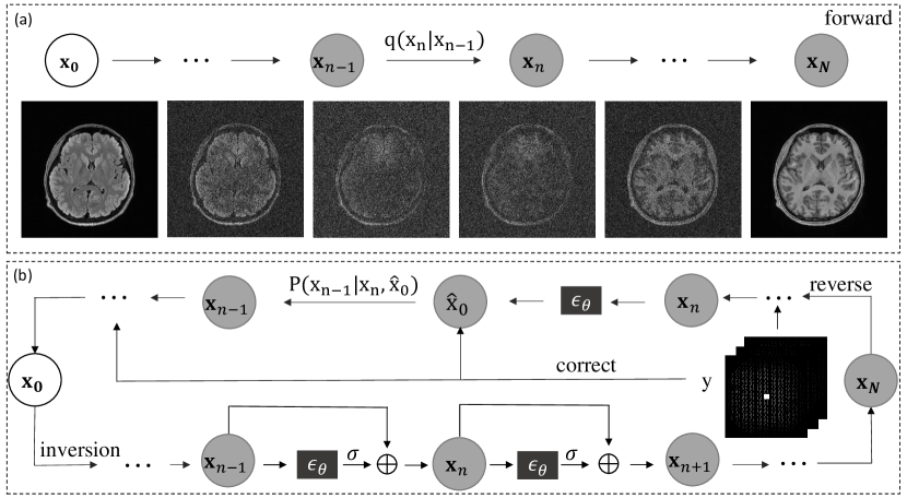
Figure 1: (a) In the forward process, $\mathbf{x}_{0}$ transitions to the distribution of $\mathbf{x}_{N}$ by gradually adding noise. (b) In the reverse process, the learned noise function $\epsilon$ maps to $\mathbf{x}_{0}$, corrects it using undersampled data, and reconstructs a high-quality $\mathbf{x}_{0}$ from $\mathbf{x}_{N}$. Further quality improvements can be achieved through the inversion process.

3.1 Guided MRI Reconstruction

The imaging model of MR reconstruction can be formulated as:

$$\mathbf{y}=\mathbf{A}\mathbf{x}+{\epsilon},$$ (11)

where $\mathbf{y}$ is the undersampled measurements in the frequency domain (i.e., $k$-space), $\mathbf{x}$ is the image to be reconstructed, $\mathbf{A}$ denotes the encoding matrix, $\mathbf{A}=\mathbf{M}\cdot\mathbf{F}\cdot\text{csm}$, $\mathbf{M}$ is the undersampling operator, $\mathbf{F}$ denotes the Fourier operator, csm denotes the coil sensitivity, and ${\epsilon}\sim\mathcal{N}(0,\sigma^{2}_{\epsilon})$. For 2D image, $\mathbf{x}\in\mathbb{C}^{n}$, $\mathbf{y}\in\mathbb{C}^{m}$ and $\mathbf{A}\in\mathbb{C}^{m\times n}$.

Since Eq. (11) is an ill-posed problem, additional prior information is necessary to solve it. Given a guiding image $\mathbf{b}$, incorporating the structural similarity prior between the guiding image and the reconstructed image, the solution to Eq. (11) can be expressed as following constrained optimization problem:

$$\min_{\mathbf{x}}R(\mathbf{x},\mathbf{b})\quad\text{subject to}\quad\mathbf{y}=\mathbf{A}\mathbf{x},$$ (12)

where $\mathbf{b}$ is the guiding image, and $R(\mathbf{x},\mathbf{b})$ represents the structural similarity prior between $\mathbf{x}$ and $\mathbf{b}$, such as group wavelet sparsity [53] and weighted similarity of intensity [54]. In traditional methods, the optimization problem is often decoupled into two subproblems that are alternately optimized to obtain the optimal solution.

Algorithm 2 Guided reconstruction

1:$\mathbf{x}_{N}\sim p_{1}$, trained $\epsilon(\cdot,\cdot;\theta)$, undersampled data $\mathbf{y}$

2:for $n=N$ to $1$ do

3:     Predict $\mathbf{x}_{0}^{\epsilon}$ using $\epsilon_{\theta}(\mathbf{x}_{n},t_{n};\theta)$

4:     CG based data consistency mapping 

5:     $\mathbf{x}_{n-1}\sim p(\mathbf{x}_{n-1}|\mathbf{x}_{0}^{\epsilon},\mathbf{x}_{n})$

6:end for

7:return $\mathbf{x}_{0}$

3.2 Guided reconstruction based on Schrödinger Bridge

Given the guiding imaging $\mathbf{b}\sim p_{1}$ and the reconstructed image $\mathbf{x}\sim p_{0}$, $R(\mathbf{x},\mathbf{b})$ can be represented as the SB prior $p(\mathbf{x}_{t})$, which diffuses between $p_{1}$ and $p_{0}$. Here, $\mathbf{x}_{t}$ is a sample along the diffusion path at time $t$. Since $p(\mathbf{x}_{t})$ is intractable, we estimate its score function through a denoised representation(Alg. 1) as an alternative and obtain denoised samples based on this representation:

$$\mathbf{x}^{\epsilon}_{0}=\mathbf{x}_{n}-\epsilon_{\theta}(\mathbf{x}_{n},t;\theta)\sigma_{n}$$ (13)

where $\epsilon_{\theta}$ represents the trained mapping function.

Then, the data consistency constraint in Eq. (12) should be applied to ensure that the generated image aligns with the acquired k-space data. There are various methods to implement data consistency mapping, including the projection method[55], gradient descent method[56] and conjugate gradient(CG)[57]. Here, we employ the CG method for this purpose. For the image $\mathbf{x}$, the Eq. (12) are reformulated, where the constraint is defined as the initial solution obtained through the denoising mapping under the SB prior:

$$\min_{\mathbf{x}}\|\mathbf{y}-\mathbf{A}\mathbf{x}\|\quad\text{subject to}\quad\mathbf{x}=\mathbf{x}^{\epsilon}_{0},$$ (14)

To solve this optimization problem, previous studies [58, 59] have verified that, under the assumption that the tangent space at the denoised sample can be represented as a Krylov subspace, using the standard CG method can ensure that the optimization direction aligns with the gradient direction of the distribution, thereby keeping the sample within the distribution $p_{0}$. Therefore, we also use the CG method in this study as:

$$\mathbf{x}_{0}=CG(\mathbf{x}^{\epsilon}_{0},\mathbf{y})$$ (15)

Since the CG correction remains on $p_{0}$ and satisfies the SB prior, iterations along the SB path can be performed to progressively refine the reconstructed image. To map the corrected sample back onto the SB path for the next iteration, we employ the posterior sampling formula:

$$p(\mathbf{x}_{n}\mid\mathbf{x}_{0},\mathbf{x}_{n+1}) =\mathcal{N}\left(\mathbf{x}_{n};\frac{\alpha_{n}^{2}}{\alpha_{n}^{2}+\sigma_{n}^{2}}\mathbf{x}_{0}+\frac{\sigma_{n}^{2}}{\alpha_{n}^{2}+\sigma_{n}^{2}}\mathbf{x}_{n+1},\right.$$

$$\quad\left.\frac{\sigma_{n}^{2}\alpha_{n}^{2}}{\alpha_{n}^{2}+\sigma_{n}^{2}}\cdot I\right),$$ (16)

where $\alpha_{n}^{2}:=\int_{t_{n}}^{t_{n+1}}\beta_{\tau}\,\mathrm{d}\tau$.

Alg. 2 illustrates the sampling algorithm.

3.3 Guided reconstruction under the inversion

Although SB provides an effective pathway for guiding between MR images with different contrasts, it inherently requires strict consistency between the guiding and reconstructed images. Otherwise, structural discrepancies may adversely affect the quality of the reconstructed image. To address this issue, we introduce an inversion strategy by refining $\mathbf{x}_{1}$ along the SB path, ensuring that its structure corresponds one-to-one with $\mathbf{x}_{0}$.

In the inversion process, a deterministic evolution process, the probability flow ODE, is used instead of the SDE to avoid introducing new randomness.

When the SDE process degenerates into the probability flow ODE, $\Sigma_{t}$ is set to 0, and $\mu_{t}$ remains unchanged. Under this condition, the posterior sampling process in Eq. (16) reduces to:

$$\mathbf{x}_{n}=\frac{\alpha_{n}^{2}}{\alpha_{n}^{2}+\sigma_{n}^{2}}\mathbf{x}_{0}+\frac{\sigma_{n}^{2}}{\alpha_{n}^{2}+\sigma_{n}^{2}}\mathbf{x}_{n+1}$$ (17)

Subsequently, to diffuse $\mathbf{x}_{n}$ into $\mathbf{x}_{n+1}$, we solve for $\mathbf{x}_{0}$ using the denoising mapping from Eq. (13) and apply it to the affine transformation form of Eq. (17):

$$\mathbf{x}_{n+1}=\mathbf{x}_{n}+\frac{\alpha_{n}^{2}\sigma_{n+1}}{\alpha_{n}^{2}+\sigma_{n}^{2}}\epsilon_{\theta}(\mathbf{x}_{n+1},n+1;\theta)$$ (18)

However, during the inversion process, the predicted noise at time $n+1$ is unknown at time $n$. A feasible solution is to use the noise predicted from time $n$ as a substitute. To this end, unify the sampling process Eq. (9) with the predicted noise objective based on the probability flow ODE:

$$\frac{\mathbf{x}_{n}-\mathbf{x}_{0}}{\sigma_{n}}=-\frac{\sigma_{n}}{\bar{\sigma}_{n}^{2}+\sigma_{n}^{2}}\mathbf{x}_{0}+\frac{\sigma_{n}}{\bar{\sigma}_{n}^{2}+\sigma_{n}^{2}}\mathbf{x}_{1},$$ (19)

where $\frac{\mathbf{x}_{n}-\mathbf{x}_{0}}{\sigma_{n}}$ can be predicted via Eq. (13). Connecting with the sampling process at time step $n+1$, the relationship between the predicted noises can be expressed as:

$$\epsilon_{\theta}(\mathbf{x}_{n+1},t+1;\theta)=\frac{\sigma_{n+1}}{\sigma_{n}}\cdot\epsilon_{\theta}(\mathbf{x}_{n},n;\theta).$$ (20)

Through Eq. (20), the noise at different time steps is correlated, thereby providing a complete and feasible inversion strategy:

$$\mathbf{x}_{n+1}=\mathbf{x}_{n}+\frac{\alpha_{n}^{2}\sigma_{n+1}^{2}}{\sigma_{n}(\alpha_{n}^{2}+\sigma_{n}^{2})}\cdot\epsilon_{\theta}(\mathbf{x}_{n},n;\theta),$$ (21)

Through the inversion strategy, the correction applied to $\mathbf{x}_{0}$ will be gradually synchronized to $\mathbf{x}_{1}$, and the corrected $\hat{\mathbf{x}}_{1}$ will have the same structural information as $\mathbf{x}_{0}$ while remaining on the correct distribution.

The inversion strategy is shown in Alg. 3. The image reconstructed by Alg. 2 is used as an initialization of $\mathbf{x}_{0}$, and the inversion strategy is applied to estimate $\hat{\mathbf{x}}_{1}$. The final image is obtained based on $\hat{\mathbf{x}}_{1}$.

Algorithm 3 Inversion reconstruction

1:$\mathbf{x}_{N}\sim p_{1}(\mathbf{x}_{N})$, $\epsilon_{\theta}(\cdot,\cdot;\theta)$, undersampled data $\mathbf{y}$

2:$\mathbf{x}_{0}$

3:for $n=N$ to $1$ do

4:     Predict $\mathbf{x}_{0}$ using $\epsilon_{\theta}(\mathbf{x}_{n},t_{n};\theta)$;

5:     CG based data consistency mapping;

6:     $\mathbf{x}_{n-1}\sim p(\mathbf{x}_{n-1}|\mathbf{x}_{0},\mathbf{x}_{n})$;

7:end for

8:$\hat{\mathbf{x}}_{0}={\mathbf{x}}_{0}$

9:for $n=1$ to $N_{i}$ do

10:     $\hat{\mathbf{x}}_{n+1}=\text{inversion}(\hat{\mathbf{x}}_{n})$;

11:end for

12:for $n=N$ to $1$ do

13:     Predict $\mathbf{x}_{0}$ using $\epsilon_{\theta}(\hat{\mathbf{x}}_{n},t_{n};\theta)$;

14:     CG based data consistency mapping;

15:     $\hat{\mathbf{x}}_{n-1}\sim p(\hat{\mathbf{x}}_{n-1}|\mathbf{x}_{0},\mathbf{x}_{n})$;

16:end for

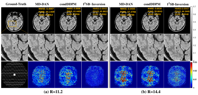
Figure 2: The reconstructed images using guided reconstruction methods with (a) $R=11.2$ and (b) $R=14.4$. The first row shows the reconstructions obtained by different methods alongside the ground truth image. The second row presents an enlarged view of the ROI, and the third row displays the error map of the reconstructions.

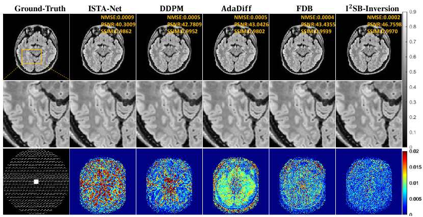
Figure 3: Direct Reconstruction results at $R=11.2$. The top row shows the ground truth and the reconstructions obtained using different methods. The second row shows an enlarged view of the ROI, and the third row displays the error map of the reconstructions.

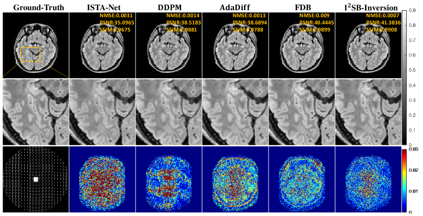
Figure 4: Direct Reconstruction results at $R=14.4$. The top row shows the ground truth and the reconstructions obtained using different methods. The second row shows an enlarged view of the ROI, and the third row displays the error map of the reconstructions.

4 Experiments

4.1 Experimental Setup

4.1.1 Experimental Data

We conducted experiments on a paired T1- and FLAIR T2-weighted image dataset, which includes fully sampled k-space data from 27 healthy volunteers. The local institutional review board approved the experiments, and informed consent was obtained from each volunteer. All data were obtained using a 3T MR scanner (uMR 790, United Imaging Healthcare, China) with a 32-channel head coil. The T1-weighted images were acquired by a 3D GRE sequence, and the FLAIR T2-weighted images were acquired using a 3D FSE sequence. For each volunteer, the position and spatial resolution were the same for both sequences with acquisition matrix = $240\times 240\times 176$ (RO × PE1 × PE2) and field of view (FOV) = $240\times 240\times 176\,\text{mm}^{3}$. Other imaging parameters were as follows. For the FLAIR-T2 sequence: $\text{TR/TE}=6000/396.4\,\text{ms}$, inversion time = 1825 ms, echo train length = 240, bandwidth = 600 Hz/Pixel, and elliptical scanning was used. The scan time was 14 minutes. For the T1 sequence: $\text{TR/TE}=7.7/3\,\text{ms}$, flip angle = 9, echo train length = 176, and bandwidth = 250 Hz/Pixel. The scan time was 8 minutes and 36 seconds.

The 3D k-space data were divided into 2D slices along the RO direction by applying the inverse Fourier transform in that direction. The first 25 and last 50 slices, which contained only background, were removed from the dataset. Then coil compression was applied to compress the data to 18 channels to reduce computational load [60]. Zero-padding was applied to increase the image size to $256\times 256$, facilitating network operations. The k-space data of T1 and T2-weighted image was retrospectively undersampled with net acceleration factors ($R$) of 11.2 and 14.4. The CAIPI undersampling scheme [61] was employed with a $48\times 48$ k-space center fully sampled. The coil sensitivity maps were estimated using the fully sampled k-space center with the ESPIRiT algorithm [62]. We randomly selected 23 volunteers for the training dataset, consisting of 4163 matched image pairs, while the remaining 4 participants formed the test dataset, comprising 724 matched image pairs.

4.1.2 Parameter Configuration

We compared our method with several SOTA methods. For guided reconstruction methods, we selected MD-DAN[37], a deep learning method based on unrolling, and Con-DDPM, a method based on conditional distribution learning (Con-DDPM is defined as a conditional DDPM guided by an image) to compare performance differences under different learning modes. Additionally, to demonstrate the advantages of guided imaging, we included a comparison with direct reconstruction methods (without guidance). For direct reconstruction methods, we selected the unrolling method ISTA-Net[22], as well as DDPM[28], AdaDiff[30], and FDB[45], which are based on distribution learning.

For unrolling methods, in ISTA-Net, the learning rate is set to 0.0001, with a batch size of 8; in MD-DAN, the batch size is 2, with a learning rate of $1\times 10^{-3}$. To ensure performance, retraining was conducted at each acceleration factor in addition to the parameter settings. For distribution learning methods, DDPM has $\beta_{\text{max}}=0.02$ and $\beta_{\text{min}}=0.0001$, and Con-DDPM shares the same configuration as DDPM. In AdaDiff, $\beta_{\text{max}}=20$, $\beta_{\text{min}}=0.1$, with the number of epochs set to 500. For FDB, the undersampling rate is 2, and the batch size is 16. In $\mathbf{I}^{2}$SB, the batch size is 32, with $\beta_{\text{max}}=0.3$ and $\beta_{\text{min}}=1\text{e}{-5}$. To ensure fairness, all experiments employed the same normalization method, which involves dividing by the maximum amplitude value.

4.1.3 Performance Evaluation

Three metrics were used to quantitatively evaluate the results, including normalized mean square error (NMSE), peak signal-to-noise ratio (PSNR), and structural similarity index (SSIM)[63].

4.2 Experimental Results

4.2.1 Guided Reconstruction Experiments

Figure 2 shows the reconstruction results at $R=11.2$ and $R=14.4$ using various guided reconstruction methods. The result of MD-DAN exhibits noticeable noise and smooth details, a common issue with unrolling-based methods. Aliasing artifacts appear on the image using con-DDPM, which can be observed on the error maps. $\mathbf{I}^{2}$SB-inversion removes substantial noise from the target, leaving noticeable noise only in fine structures. Among these, $\mathbf{I}^{2}$SB-inversion achieves the best visual performance, with the highest quantitative metrics among the compared methods.

Table 1: Gudied Reconstruction experiments. The average quantitative metrics at absolutely $R=11.2$ and $R=14.4$.

AF	Method	NMSE (%)	PSNR (dB)	SSIM (%)
11.2	MD-DAN	0.24 $\pm$ 0.25	43.03 $\pm$ 3.09	97.44 $\pm$ 1.36
	conDDPM	0.17 $\pm$ 0.18	45.11 $\pm$ 3.59	97.76 $\pm$ 1.31
	$\mathbf{I}^{2}$SB-inversion	0.08 $\pm$ 0.09	48.26 $\pm$ 3.09	99.18 $\pm$ 0.89
14.4	MD-DAN	0.89 $\pm$ 0.79	37.05 $\pm$ 2.94	94.47 $\pm$ 1.94
	conDDPM	0.35 $\pm$ 0.40	42.11 $\pm$ 4.23	96.71 $\pm$ 1.73
	$\mathbf{I}^{2}$SB-inversion	0.26 $\pm$ 0.28	43.20 $\pm$ 3.90	98.28 $\pm$ 1.38

Table 2: Direct reconstruction experiment. The average quantitative metrics at absolutely $R=11.2$ and $R=14.4$.

AF	Method	NMSE (%)	PSNR (dB)	SSIM (%)
11.2	ISTA-Net	0.20 $\pm$ 0.19	43.73 $\pm$ 3.01	97.69 $\pm$ 1.94
	DDPM	0.23 $\pm$ 0.22	43.48 $\pm$ 3.36	97.11 $\pm$ 1.50
	AdaDiff	0.20 $\pm$ 0.25	44.59 $\pm$ 3.60	97.03 $\pm$ 1.59
	FDB	0.17 $\pm$ 0.38	45.21 $\pm$ 3.15	98.50 $\pm$ 1.57
	$\mathbf{I}^{2}$SB-inversion	0.08 $\pm$ 0.09	48.26 $\pm$ 3.09	99.18 $\pm$ 0.89
14.4	ISTA-Net	0.65 $\pm$ 0.47	38.07 $\pm$ 2.93	95.95 $\pm$ 2.46
	DDPM	0.43 $\pm$ 0.46	41.12 $\pm$4.14	96.15$\pm$ 1.87
	AdaDiff	0.54 $\pm$ 0.69	40.58 $\pm$ 4.38	96.30 $\pm$ 1.89
	FDB	0.32 $\pm$ 0.67	42.25 $\pm$ 3.25	97.87 $\pm$ 1.87
	$\mathbf{I}^{2}$SB-inversion	0.26 $\pm$ 0.28	43.20 $\pm$ 3.90	98.28 $\pm$ 1.38

4.2.2 Direct Reconstruction Experiments

We also compared $\mathbf{I}^{2}$SB with reconstruction methods without guidance. Fig. 3 shows the reconstruction results using ISTA-Net, DDPM, AdaDiff, FDB, and $\mathbf{I}^{2}$SB-inversion at $R=11.2$. ISTA-Net and DDPM exhibit aliasing artifacts in their reconstructed images, as highlighted in their respective error maps. Compared to $\mathbf{I}^{2}$SB-inversion, AdaDiff and FDB show larger reconstruction errors. $\mathbf{I}^{2}$SB-inversion achieves the highest quantitative metrics and superior reconstruction quality. Fig. 4 shows the reconstruction results at $R=14.4$. At this high acceleration rate, aliasing artifacts appear in the images reconstructed by ISTA-Net, DDPM, AdaDiff, and FDB. In contrast, $\mathbf{I}^{2}$SB-inversion maintains high reconstruction quality and achieves the best quantitative metrics. The average quantitative metrics are summarized in Table 2, where $\mathbf{I}^{2}$SB-inversion consistently outperforms the other methods.

5 Discussion

5.1 The effect of inversion strategy

To validate the effectiveness of the Inversion strategy and its contribution to the model’s acceleration capability, we conducted tests on $\mathbf{I}^{2}$SB-Inversion and $\mathbf{I}^{2}$SB-Recon (without the Inversion strategy) under acceleration rates $R=11.2,14.4,18.9,23.2$, and $28.4$. Fig. 5 shows the performance comparison with and without the Inversion strategy under different acceleration rates. The experimental results demonstrate that the Inversion strategy significantly improves performance, with its advantages being particularly evident at high acceleration rates (e.g., $R=28.4$).

Furthermore, Fig. 6 shows the reconstruction results at an acceleration rate of $R=18.9$. At nearly 20-fold acceleration, $\mathbf{I}^{2}$SB-Inversion more effectively preserves fine structures and significantly suppresses global noise, whereas $\mathbf{I}^{2}$SB-Recon shows relatively weaker noise suppression. The difference map between $\mathbf{I}^{2}$SB-Inversion and $\mathbf{I}^{2}$SB-Recon indicates that the Inversion strategy not only reduces noise but also enhances fine structures. However, when the acceleration rate exceeds 20 or approaches 30, the limited k-space information constrains the recovery of details. Even though the Inversion strategy remains effective, the overall reconstruction performance is still restricted.

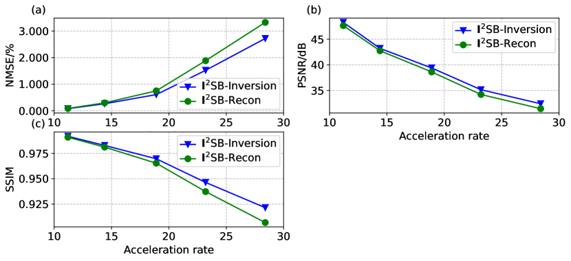
Figure 5: The performance comparison between $\mathbf{I}^{2}$SB-Recon and $\mathbf{I}^{2}$SB-Inversion under acceleration rates $R=11.2,14.4,18.9,23.2$ and $28.4$ is shown below. Fig (a), (b), and (c) present the NMSE, PSNR, and SSIM metrics for the reconstruction results respectively.

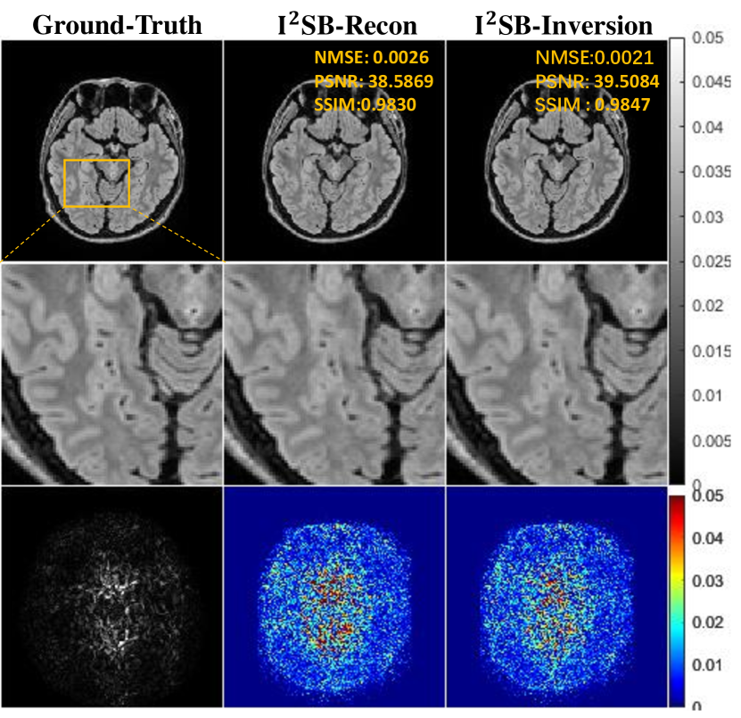
Figure 6: Ablation study of reconstruction results at an acceleration factor of $R=18.9$. The top row shows the ground truth and the reconstructions obtained using different methods. The second row shows an enlarged view of the ROI. The third row displays the difference map between the $\mathbf{I}^{2}$SB-Inversion and $\mathbf{I}^{2}$SB-Recon, as well as the error maps between the reconstructions and the ground truth.

5.2 Extension of Multi-modal Guided Reconstruction

Equation Eq. (12) can be generalized to represent a common multi-modal guided reconstruction problem, where $\mathbf{y}$, $\mathbf{x}$, and $\mathbf{b}$ denote, respectively, the observed signal, the signal to be reconstructed, and the guiding signal. In reconstruction, two main types of challenges are often encountered:

5.2.1 Problems with Known Forward Operator $\mathbf{A}$ (e.g., Medical Image Reconstruction)

When the forward operator $\mathbf{A}$ is known, as in medical image reconstruction tasks, $\mathbf{I}^{2}$SB-inversion can be applied across a variety of guided reconstruction models. Typical scenarios include MRI, CT[64], and ultrasound reconstruction[65]. In such cases, other structural medical images (e.g., PET) can be used as guidance to assist with reconstruction modes that require longer acquisition times, without incurring additional scanning burdens. For example, PET-CT systems can acquire PET and CT data simultaneously, making it well-suited for multi-modal imaging needs.

5.2.2 Problems with Unknown or Non-invertible Forward Operator $\mathbf{A}$

In some cases, the forward operator $\mathbf{A}$ may be unknown or non-invertible, such as in blind image restoration[66], where reconstruction occurs without a known imaging model. For such cases, approximate solutions can be achieved by appropriately designing inverse problems or by optimizing with a specific loss function via gradient descent.

In summary, $I^{2}$SB-inversion extends to diverse applications with known or approximate forward operators, achieving high-precision multi-modal image translation by aligning guiding and target image structures.

5.3 Limitations

This study incorporates a inversion strategy into guided reconstruction to correct structural differences, but this is limited to correcting the differences from the data perspective, without enhancing the parametric denoising mapping capabilities. For mapping enhancement, our future work will focus on two aspects:

1. Adaptive fine-tuning of weights during reconstruction. The mapping weights are fine-tuned based on a corrected single paired sample, and then a weighted combination with the initial weights is used as the final mapping.

2. Feature layer embedding optimization of the mapping based on corrected data. Features from the corrected data are introduced into the mapping network decoder layer via an attention mechanism as guidance during reconstruction, reducing uncertainty to enhance the mapping.

6 Conclusions

In this paper, we propose a novel guided reconstruction framework based on the Schrödinger Bridge, named $\mathbf{I}^{2}$SB-inversion. To address the challenge of accommodating structural differences in multi-contrast images, we introduce an innovative inversion strategy from image editing, enabling correction of the guiding image to enhance structural alignment. Experimental results demonstrate that our method significantly improves reconstruction accuracy and stability on the paired T1 and T2-FLAIR dataset, confirming its effectiveness and superiority.

7 Acknowledgments

This study was supported in part by the National Natural Science Foundation of China under grant nos. 62322119, 12226008, 52293425, 62125111, 62106252, 12026603, 62206273, 62476268; the National Key R&D Program of China nos. 2021YFF0501402, 2023YFA1011403; the Key Laboratory for Magnetic Resonance and Multimodality Imaging of Guangdong Province under grant no. 2023B1212060052; and the Shenzhen Science and Technology Program under grant nos. RCYX20210609104444089, JCYJ20220818101205012.

References

- [1] M. Lustig, D. L. Donoho, J. M. Santos, and J. M. Pauly, “Compressed sensing mri,” IEEE signal processing magazine, vol. 25, no. 2, pp. 72–82, 2008.
- [2] J. P. Haldar, D. Hernando, and Z.-P. Liang, “Compressed-sensing mri with random encoding,” IEEE transactions on Medical Imaging, vol. 30, no. 4, pp. 893–903, 2010.
- [3] M. J. Ehrhardt, K. Thielemans, L. Pizarro, D. Atkinson, S. Ourselin, B. F. Hutton, and S. R. Arridge, “Joint reconstruction of pet-mri by exploiting structural similarity,” Inverse Problems, vol. 31, no. 1, p. 015001, 2014.
- [4] B. Zhao, J. P. Haldar, A. G. Christodoulou, and Z.-P. Liang, “Image reconstruction from highly undersampled (k, t)-space data with joint partial separability and sparsity constraints,” IEEE transactions on medical imaging, vol. 31, no. 9, pp. 1809–1820, 2012.
- [5] A. Majumdar, “Improving synthesis and analysis prior blind compressed sensing with low-rank constraints for dynamic mri reconstruction,” Magnetic resonance imaging, vol. 33, no. 1, pp. 174–179, 2015.
- [6] P. J. Shin, P. E. Larson, M. A. Ohliger, M. Elad, J. M. Pauly, D. B. Vigneron, and M. Lustig, “Calibrationless parallel imaging reconstruction based on structured low-rank matrix completion,” Magnetic resonance in medicine, vol. 72, no. 4, pp. 959–970, 2014.
- [7] S. G. Lingala, Y. Hu, E. DiBella, and M. Jacob, “Accelerated dynamic mri exploiting sparsity and low-rank structure: kt slr,” IEEE transactions on medical imaging, vol. 30, no. 5, pp. 1042–1054, 2011.
- [8] K. H. Jin, D. Lee, and J. C. Ye, “A general framework for compressed sensing and parallel mri using annihilating filter based low-rank hankel matrix,” IEEE Transactions on Computational Imaging, vol. 2, no. 4, pp. 480–495, 2016.
- [9] C. Y. Lin and J. A. Fessler, “Efficient dynamic parallel mri reconstruction for the low-rank plus sparse model,” IEEE transactions on computational imaging, vol. 5, no. 1, pp. 17–26, 2018.
- [10] J. D. Trzasko and A. Manduca, “Highly undersampled magnetic resonance image reconstruction via homotopic -minimization,” IEEE Transactions on Medical Imaging, vol. 28, no. 1, pp. 106–121, 2008.
- [11] A. C. Yang, M. Kretzler, S. Sudarski, V. Gulani, and N. Seiberlich, “Sparse reconstruction techniques in magnetic resonance imaging: methods, applications, and challenges to clinical adoption,” Investigative radiology, vol. 51, no. 6, pp. 349–364, 2016.
- [12] J. Huang, A. I. Aviles-Rivero, C.-B. Schönlieb, and G. Yang, “Vigu: Vision gnn u-net for fast mri,” in 2023 IEEE 20th International Symposium on Biomedical Imaging (ISBI). IEEE, 2023, pp. 1–5.
- [13] P. Huang, C. Zhang, X. Zhang, X. Li, L. Dong, and L. Ying, “Unsupervised deep unrolled reconstruction using regularization by denoising,” arXiv preprint arXiv:2205.03519, 2022.
- [14] D. Liang, J. Cheng, Z. Ke, and L. Ying, “Deep magnetic resonance image reconstruction: Inverse problems meet neural networks,” IEEE Signal Processing Magazine, vol. 37, no. 1, pp. 141–151, 2020.
- [15] Y. Han, L. Sunwoo, and J. C. Ye, “k-space deep learning for accelerated mri,” IEEE Transactions on Medical Imaging, vol. 39, no. 2, pp. 377–386, 2019.
- [16] X. Peng, B. P. Sutton, F. Lam, and Z.-P. Liang, “Deepsense: Learning coil sensitivity functions for sense reconstruction using deep learning,” Magnetic Resonance in Medicine, vol. 87, no. 4, pp. 1894–1902, 2022.
- [17] G. Oh, B. Sim, H. Chung, L. Sunwoo, and J. C. Ye, “Unpaired deep learning for accelerated mri using optimal transport driven cyclegan,” IEEE Transactions on Computational Imaging, vol. 6, pp. 1285–1296, 2020.
- [18] U. Nakarmi, J. Y. Cheng, E. P. Rios, M. Mardani, J. M. Pauly, L. Ying, and S. S. Vasanawala, “Multi-scale unrolled deep learning framework for accelerated magnetic resonance imaging,” in 2020 IEEE 17th International Symposium on Biomedical Imaging (ISBI). IEEE, 2020, pp. 1056–1059.
- [19] P. Huang, C. Zhang, H. Li, S. K. Gaire, R. Liu, X. Zhang, X. Li, and L. Ying, “Deep mri reconstruction without ground truth for training,” in Proceedings of 27th Annual Meeting of ISMRM, 2019.
- [20] H. K. Aggarwal, M. P. Mani, and M. Jacob, “Modl: Model-based deep learning architecture for inverse problems,” IEEE Transactions on Medical Imaging, vol. 38, no. 2, pp. 394–405, 2018.
- [21] J. Sun, H. Li, Z. Xu et al., “Deep admm-net for compressive sensing mri,” Advances in neural information processing systems, vol. 29, 2016.
- [22] J. Zhang and B. Ghanem, “Ista-net: Interpretable optimization-inspired deep network for image compressive sensing,” in Proceedings of the IEEE conference on computer vision and pattern recognition, 2018, pp. 1828–1837.
- [23] Z.-X. Cui, J. Cheng, Q. Zhu, Y. Liu, S. Jia, K. Zhao, Z. Ke, W. Huang, H. Wang, Y. Zhu et al., “Equilibrated zeroth-order unrolled deep networks for accelerated mri,” arXiv preprint arXiv:2112.09891, 2021.
- [24] Z. Ke, W. Huang, Z.-X. Cui, J. Cheng, S. Jia, H. Wang, X. Liu, H. Zheng, L. Ying, Y. Zhu et al., “Learned low-rank priors in dynamic mr imaging,” IEEE Transactions on Medical Imaging, vol. 40, no. 12, pp. 3698–3710, 2021.
- [25] W. Huang, Z. Ke, Z.-X. Cui, J. Cheng, Z. Qiu, S. Jia, L. Ying, Y. Zhu, and D. Liang, “Deep low-rank plus sparse network for dynamic mr imaging,” Medical Image Analysis, vol. 73, p. 102190, 2021.
- [26] J. Cheng, W. Huang, Z. Cui, Z. Ke, L. Ying, H. Wang, Y. Zhu, and D. Liang, “Learning data consistency for mr dynamic imaging,” Learning, 2020.
- [27] Y. Song and S. Ermon, “Generative modeling by estimating gradients of the data distribution,” Advances in neural information processing systems, vol. 32, 2019.
- [28] J. Ho, A. Jain, and P. Abbeel, “Denoising diffusion probabilistic models,” Advances in neural information processing systems, vol. 33, pp. 6840–6851, 2020.
- [29] Y. Song, J. Sohl-Dickstein, D. P. Kingma, A. Kumar, S. Ermon, and B. Poole, “Score-based generative modeling through stochastic differential equations,” arXiv preprint arXiv:2011.13456, 2020.
- [30] A. Güngör, S. U. Dar, Ş. Öztürk, Y. Korkmaz, H. A. Bedel, G. Elmas, M. Ozbey, and T. Çukur, “Adaptive diffusion priors for accelerated mri reconstruction,” Medical image analysis, vol. 88, p. 102872, 2023.
- [31] H. Chung and J. C. Ye, “Score-based diffusion models for accelerated mri,” Medical image analysis, vol. 80, p. 102479, 2022.
- [32] H. Chung, J. Kim, M. T. Mccann, M. L. Klasky, and J. C. Ye, “Diffusion posterior sampling for general noisy inverse problems,” arXiv preprint arXiv:2209.14687, 2022.
- [33] H. Chung, B. Sim, D. Ryu, and J. C. Ye, “Improving diffusion models for inverse problems using manifold constraints,” Advances in Neural Information Processing Systems, vol. 35, pp. 25 683–25 696, 2022.
- [34] Z.-X. Cui, C. Cao, J. Cheng, S. Jia, H. Zheng, D. Liang, and Y. Zhu, “Spirit-diffusion: Self-consistency driven diffusion model for accelerated mri,” arXiv preprint arXiv:2304.05060, 2023.
- [35] Z.-X. Cui, C. Liu, X. Fan, C. Cao, J. Cheng, Q. Zhu, Y. Liu, S. Jia, Y. Zhou, H. Wang et al., “Physics-informed deepmri: Bridging the gap from heat diffusion to k-space interpolation,” arXiv preprint arXiv:2308.15918, 2023.
- [36] Y. Xie and Q. Li, “Measurement-conditioned denoising diffusion probabilistic model for under-sampled medical image reconstruction,” in International Conference on Medical Image Computing and Computer-Assisted Intervention. Springer, 2022, pp. 655–664.
- [37] Y. Yang, N. Wang, H. Yang, J. Sun, and Z. Xu, “Model-driven deep attention network for ultra-fast compressive sensing mri guided by cross-contrast mr image,” in Medical Image Computing and Computer Assisted Intervention–MICCAI 2020: 23rd International Conference, Lima, Peru, October 4–8, 2020, Proceedings, Part II 23. Springer, 2020, pp. 188–198.
- [38] M. Özbey, O. Dalmaz, S. U. Dar, H. A. Bedel, Ş. Özturk, A. Güngör, and T. Çukur, “Unsupervised medical image translation with adversarial diffusion models,” IEEE Transactions on Medical Imaging, 2023.
- [39] T. Xie, Z.-X. Cui, C. Luo, H. Wang, C. Liu, Y. Zhang, X. Wang, Y. Zhu, G. Chen, D. Liang et al., “Joint diffusion: mutual consistency-driven diffusion model for pet-mri co-reconstruction,” Physics in Medicine & Biology, vol. 69, no. 15, p. 155019, 2024.
- [40] X. Meng, K. Sun, J. Xu, X. He, and D. Shen, “Multi-modal modality-masked diffusion network for brain mri synthesis with random modality missing,” IEEE Transactions on Medical Imaging, 2024.
- [41] Z. Li, D. Chang, Z. Zhang, F. Luo, Q. Liu, J. Zhang, G. Yang, and W. Wu, “Dual-domain collaborative diffusion sampling for multi-source stationary computed tomography reconstruction,” IEEE Transactions on Medical Imaging, 2024.
- [42] C. Yang, D. Sheng, B. Yang, W. Zheng, and C. Liu, “A dual-domain diffusion model for sparse-view ct reconstruction,” IEEE Signal Processing Letters, 2024.
- [43] G.-H. Liu, A. Vahdat, D.-A. Huang, E. A. Theodorou, W. Nie, and A. Anandkumar, “I2sb: Image-to-image schrödinger bridge,” arXiv preprint arXiv:2302.05872, 2023.
- [44] B. Kim, G. Kwon, K. Kim, and J. C. Ye, “Unpaired image-to-image translation via neural schr” odinger bridge,” arXiv preprint arXiv:2305.15086, 2023.
- [45] M. U. Mirza, O. Dalmaz, H. A. Bedel, G. Elmas, Y. Korkmaz, A. Gungor, S. U. Dar, and T. Çukur, “Learning fourier-constrained diffusion bridges for mri reconstruction,” 2023.
- [46] A. Kendall and Y. Gal, “What uncertainties do we need in bayesian deep learning for computer vision?” Advances in neural information processing systems, vol. 30, 2017.
- [47] I. Huberman-Spiegelglas, V. Kulikov, and T. Michaeli, “An edit friendly ddpm noise space: Inversion and manipulations,” in Proceedings of the IEEE/CVF Conference on Computer Vision and Pattern Recognition, 2024, pp. 12 469–12 478.
- [48] E. Schrödinger, “Sur la théorie relativiste de l’électron et l’interprétation de la mécanique quantique,” in Annales de l’institut Henri Poincaré, vol. 2, no. 4, 1932, pp. 269–310.
- [49] C. Léonard, “A survey of the schr” odinger problem and some of its connections with optimal transport,” arXiv preprint arXiv:1308.0215, 2013.
- [50] T. Chen, G.-H. Liu, and E. A. Theodorou, “Likelihood training of schr” odinger bridge using forward-backward sdes theory,” arXiv preprint arXiv:2110.11291, 2021.
- [51] D. Fernandes, F. Vargas, C. H. Ek, and N. Campbell, “Shooting schrödinger’s cat,” in Symposium on Advances in Approximate Bayesian Inference (AABI), 2022.
- [52] C. Zhang, S. Bengio, M. Hardt, B. Recht, and O. Vinyals, “Understanding deep learning (still) requires rethinking generalization,” Communications of the ACM, vol. 64, no. 3, pp. 107–115, 2021.
- [53] J. Huang, C. Chen, and L. Axel, “Fast multi-contrast mri reconstruction,” Magnetic resonance imaging, vol. 32, no. 10, pp. 1344–1352, 2014.
- [54] L. Weizman, Y. C. Eldar, and D. Ben Bashat, “Reference-based mri,” Medical physics, vol. 43, no. 10, pp. 5357–5369, 2016.
- [55] M. A. Griswold, P. M. Jakob, R. M. Heidemann, M. Nittka, V. Jellus, J. Wang, B. Kiefer, and A. Haase, “Generalized autocalibrating partially parallel acquisitions (grappa),” Magnetic Resonance in Medicine: An Official Journal of the International Society for Magnetic Resonance in Medicine, vol. 47, no. 6, pp. 1202–1210, 2002.
- [56] M. Lustig, D. Donoho, and J. M. Pauly, “Sparse mri: The application of compressed sensing for rapid mr imaging,” Magnetic Resonance in Medicine: An Official Journal of the International Society for Magnetic Resonance in Medicine, vol. 58, no. 6, pp. 1182–1195, 2007.
- [57] K. P. Pruessmann, M. Weiger, M. B. Scheidegger, and P. Boesiger, “Sense: sensitivity encoding for fast mri,” Magnetic Resonance in Medicine: An Official Journal of the International Society for Magnetic Resonance in Medicine, vol. 42, no. 5, pp. 952–962, 1999.
- [58] H. Chung, S. Lee, and J. C. Ye, “Decomposed diffusion sampler for accelerating large-scale inverse problems,” arXiv preprint arXiv:2303.05754, 2023.
- [59] Y. Zhu, K. Zhang, J. Liang, J. Cao, B. Wen, R. Timofte, and L. Van Gool, “Denoising diffusion models for plug-and-play image restoration,” in Proceedings of the IEEE/CVF Conference on Computer Vision and Pattern Recognition, 2023, pp. 1219–1229.
- [60] T. Zhang, J. M. Pauly, S. S. Vasanawala, and M. Lustig, “Coil compression for accelerated imaging with cartesian sampling,” Magnetic resonance in medicine, vol. 69, no. 2, pp. 571–582, 2013.
- [61] F. A. Breuer, M. Blaimer, R. M. Heidemann, M. F. Mueller, M. A. Griswold, and P. M. Jakob, “Controlled aliasing in parallel imaging results in higher acceleration (caipirinha) for multi-slice imaging,” Magnetic Resonance in Medicine: An Official Journal of the International Society for Magnetic Resonance in Medicine, vol. 53, no. 3, pp. 684–691, 2005.
- [62] M. Uecker, P. Lai, M. J. Murphy, P. Virtue, M. Elad, J. M. Pauly, S. S. Vasanawala, and M. Lustig, “Espirit—an eigenvalue approach to autocalibrating parallel mri: where sense meets grappa,” Magnetic Resonance in Medicine, vol. 71, no. 3, pp. 990–1001, 2014.
- [63] Z. Wang, A. C. Bovik, H. R. Sheikh, and E. P. Simoncelli, “Image quality assessment: from error visibility to structural similarity,” IEEE Transactions on Image Processing, vol. 13, no. 4, pp. 600–612, 2004.
- [64] J. Liu, R. Anirudh, J. J. Thiagarajan, S. He, K. A. Mohan, U. S. Kamilov, and H. Kim, “Dolce: A model-based probabilistic diffusion framework for limited-angle ct reconstruction,” in Proceedings of the IEEE/CVF International Conference on Computer Vision, 2023, pp. 10 498–10 508.
- [65] Y. Zhang, C. Huneau, J. Idier, and D. Mateus, “Ultrasound image reconstruction with denoising diffusion restoration models,” in International Conference on Medical Image Computing and Computer-Assisted Intervention. Springer, 2023, pp. 193–203.
- [66] H. Chung, J. Kim, S. Kim, and J. C. Ye, “Parallel diffusion models of operator and image for blind inverse problems,” in Proceedings of the IEEE/CVF Conference on Computer Vision and Pattern Recognition, 2023, pp. 6059–6069.