Investigating the universality of five-point QCD scattering amplitudes at high energy

Abstract

We investigate $2\to 3$ QCD scattering amplitudes in multi-Regge kinematics, i.e. where the final partons are strongly ordered in rapidity. In this regime amplitudes exhibit intriguing factorisation properties which can be understood in terms of effective degrees of freedom called reggeons. Working within the Balitsky/JIMWLK framework, we predict these amplitudes for the first time to next-to-next-to-leading logarithmic order, and compare against the limit of QCD scattering amplitudes in full colour and kinematics. We find that the latter can be described in terms of universal objects, and that the apparent non-universality arising at NNLL comes from well-defined and under-control contributions that we can predict. Thanks to this observation, we extract for the first time the universal vertex that controls the emission of the central-rapidity gluon, both in QCD and $\mathcal{N}=4$ super Yang-Mills.

1 Introduction

Scattering processes in the high-energy – or Regge – limit offer a rich laboratory to explore properties of gauge theories, both at amplitude and cross-section level. In this regime, the invariant mass of any pair of final-state particles grows with the scattering energy $\sqrt{s}$ and it is much larger than their individual transverse momenta that are instead held fixed. This can equivalently be expressed by requiring that the final-state particles are strongly ordered in rapidity while having comparable transverse momenta. Such a configuration for $2\to n$ scattering is referred to as multi-Regge kinematics (MRK). In this scenario, scattering amplitudes feature interesting properties, the most remarkable one being the phenomenon of reggeisation: they naturally organise in terms of $t$-channel exchanges of effective degrees of freedom called $reggeons$, whose propagator is dressed with a power-law behaviour $s^{\tau}$. In perturbative QCD, or more generally in non-abelian gauge theories, the dominant contribution is given by a reggeised gluon, whose power-law behaviour is controlled by the gluon Regge trajectory $\tau_{g}$.

Following the seminal work by Fadin, Kuraev and Lipatov on the reggeisation of gauge bosons in non-abelian gauge theories with broken symmetries Fadin:1975cb ; Lipatov:1976zz , the investigation of QCD as a massless theory came shortly after Kuraev:1976ge ; Kuraev:1977fs ; Balitsky:1978ic . These studies led to the conception of the celebrated Balitsky-Fadin-Kuraev-Lipatov (BFKL) formalism and its related evolution equation. The latter allows for the resummation of large terms of type $\ln(s/|t|)$ arising in the Regge limit at any order in perturbative QCD, both at leading-logarithmic (LL) Fadin:1975cb ; Lipatov:1976zz ; Kuraev:1976ge ; Kuraev:1977fs ; Balitsky:1978ic , i.e. $\left[\alpha_{s}\ln(s/|t|)\right]^{n}$, and next-to-leading-logarithmic (NLL) accuracy Fadin:1998py ; Ciafaloni:1998gs ; Kotikov:2000pm , i.e. $\alpha_{s}\left[\alpha_{s}\ln(s/|t|)\right]^{n}$. Apart from its formal interest, the BFKL formalism has a broad spectrum of applications, ranging from the physics of small-$x$ parton distribution functions, see e.g. refs Jaroszewicz:1982gr ; Catani:1990eg ; Altarelli:2001ji ; Ciafaloni:2003ek , to the phenomenology of processes with large rapidity gaps in hadronic collisions, see e.g. refs Mueller:1986ey ; DelDuca:1993mn ; Stirling:1994he ; Andersen:2001kta ; Colferai:2010wu ; Ducloue:2013hia ; Caporale:2014gpa ; Andersen:2011hs ; Andersen:2023kuj . Improving the BFKL approach beyond the current frontier to reach next-to-next-to-leading-logarithmic (NNLL) accuracy, i.e. $\alpha_{s}^{2}\left[\alpha_{s}\ln(s/|t|)\right]^{n}$, would significantly enhance those studies and our understanding of QCD in extreme regimes.

The BFKL formalism relies on fundamental properties of scattering amplitudes in the high-energy regime. At LL accuracy, amplitudes are described to all-orders in perturbation theory as a tree-level exchange of reggeised gluons in the $t$-channel, whose power-law behaviour is fully determined by the one-loop Regge trajectory. In MRK, the interaction between these reggeons and the gluons emitted centrally in the large rapidity gap is described by an effective vertex known as the Lipatov or central-emission vertex (CEV) Lipatov:1976zz . Owing to single-reggeon exchanges in the $t$-channels, scattering amplitudes have a simple pole in the complex-angular momentum plane Collins:1977jy ; Ioffe:2010zz . Thus, at LL accuracy, the iterated structure of reggeon propagators and CEVs goes under the name of Regge-pole factorisation. Starting at NLL, multi-reggeon exchanges appear and they give rise to cuts in the complex-angular momentum plane. However, these contribute solely to the absorptive (imaginary) part of the amplitude, whereas the dispersive (real) part is still described as a single reggeon exchange, thus showing a Regge-pole factorisation behaviour Fadin:1998py . At this logarithmic order, the factorised structure also entails the interaction between a single reggeon and the particles that sit at the edges of the large rapidity gap, defining the so-called impact factors. The latter are flavour-dependent, and in QCD, there are impact factors for both quarks and gluons. It is worth stressing that these are the only process-dependent ingredients in Regge-pole factorisation. Once they are accounted for, this factorisation reflects into a statement about Regge-pole universality in (M)RK.

Several ingredients required for predictions in the BFKL formalism beyond LL accuracy are known. Two-loop corrections to the gluon Regge trajectory were computed long ago Fadin:1996tb , and more recently three-loop ones in both $\mathcal{N}=4$ super Yang-Mills (sYM) Henn:2016jdu and full QCD DelDuca:2021vjq ; Caola:2021izf ; Falcioni:2021dgr became available. One-loop QCD corrections to the quark and gluon impact factors were computed in refs. Fadin:1992zt ; Fadin:1993wh ; Fadin:1993qb ; Bern:1998sc ; DelDuca:1998kx ; Fadin:1999de and two-loop ones appeared in ref. Caron-Huot:2017fxr . Finally, the CEV is known with one-loop accuracy in QCD Fadin:1993wh ; Fadin:1994fj ; Fadin:1996yv ; DelDuca:1998cx , and it was recently presented in dimensional regularisation up to second order in the regulator Fadin:2023roz . The only missing components required for computing the Regge-pole contribution to scattering amplitudes at NNLL are the one-loop corrections to the central two-gluon emission vertex, and the two-loop ones to the CEV. While the former has been recently presented in $\mathcal{N}=4$ sYM Byrne:2022wzk , the latter is unknown.

Alongside the evaluation of these contributions, an outstanding issue in QCD that prevents a robust generalisation of the BFKL framework beyond NLL is the appearance of cuts in the complex angular momentum plane. These are understood as multi-reggeon exchanges. Starting from NNLL, such cuts also appear in the dispersive part of the result, making the identification of the Regge pole contribution problematic. High-energy factorisation breaking at NNLL in the real part of two-loop $2\to 2$ QCD scattering amplitudes was first reported in ref. DelDuca:2001gu . The observation that factorisation-violating terms are infrared (IR) divergent motivated investigations into their contributions to the IR poles of scattering amplitudes at two- and three-loop orders in QCD DelDuca:2013ara ; DelDuca:2014cya . In the recent past, several approaches have appeared to address this problem in a systematic way. Ref. Caron-Huot:2013fea developed an effective theory based on the Balitsky/JIMWLK formalism Balitsky:1995ub ; Jalilian-Marian:1997qno ; Jalilian-Marian:1997jhx ; Jalilian-Marian:1997ubg ; Kovner:2000pt ; Weigert:2000gi ; Iancu:2000hn ; Iancu:2001ad ; Ferreiro:2001qy ; Caron-Huot:2013fea that paved the way for many amplitude-level investigations, see e.g. Caron-Huot:2017fxr ; Caron-Huot:2020grv ; Falcioni:2020lvv ; Falcioni:2021buo ; Falcioni:2021dgr . Fadin and Lipatov studied instead the complete contribution of three-reggeon cuts to the $2\to 2$ scattering amplitude, using a diagrammatic approach Fadin:2017nka ; Fadin:2019tdt ; Fadin:2021csi ; Fadin:2024eyf . More recently, a SCET-based formalism based on Glauber exchanges has also been developed Rothstein:2016bsq ; Rothstein:2024fpx ; Moult:2022lfy ; Gao:2024qsg .

Thanks to impressive progress on the calculation of multi-loop multi-leg scattering amplitudes Abreu:2018aqd ; Caron-Huot:2020vlo ; Caola:2021izf ; Caola:2022dfa ; Agarwal:2023suw ; DeLaurentis:2023izi ; DeLaurentis:2023nss , we now have analytic data that allow us to $a)$ validate the approaches described above, $b)$ gain direct insight into the high-energy structure of perturbative QCD, $c)$ extract the universal building blocks required to extend the BFKL programme beyond NLL accuracy. In this paper, we take an important step in this direction by considering the high-energy limit of the $2\to 3$ QCD scattering amplitudes in full colour and kinematics Agarwal:2023suw ; DeLaurentis:2023izi ; DeLaurentis:2023nss and comparing them against predictions that we obtained from the framework of ref. Caron-Huot:2013fea . By matching against the EFT Caron-Huot:2013fea , we both validate this approach at NNLL in MRK at the two-loop level, and extract for the first time the universal two-loop vertex that describes the emission of a central-rapidity gluon. This can be seen as a crucial step towards a robust definition of the Lipatov vertex at two loops and beyond.

The remainder of this paper is organised as follows: in section 2 we discuss the $2\to 3$ MRK, list the contributing partonic channels, describe aspects related to signature and colour and illustrate how we expanded the five-point QCD scattering amplitudes Agarwal:2023suw in MRK. Section 3 is devoted to a review of the Balitsky/JIMWLK formalism and to a discussion of how it can be used to predict the form of our scattering amplitudes in MRK. We do this by extending the results of ref. Caron-Huot:2013fea and expressing the two-loop scattering amplitude in terms of fully-predicted quantities and one unknown two-loop universal vertex that describes the emission of the central-rapidity gluon. In section 4 we compare the results from sections 2 and 3. After finding full agreement between the two for all the terms that we predict unambiguously at NNLL, we leverage the knowledge of the full $2\to 3$ QCD amplitude to extract for the first time the two-loop universal vertex, both in QCD and $\mathcal{N}=4$ sYM. Moreover, we exploit the well-known IR structure of two-loop gauge-theory amplitudes to define finite remainders for their universal building blocks in the high-energy regime. We also document the various checks that we have performed to validate our calculations. We present our conclusions, final remarks and outlook in section 5.

2 Five-point scattering amplitudes in MRK

In this section we discuss the defining features of five-point scattering amplitudes in MRK. We begin with a precise description of the kinematics, and then turn to the discussion of signature eigenstates as well as the choice of appropriate colour bases for the various partonic channels. In the second half we describe how we obtain the high-energy limit of $2\to 3$ amplitudes up to two loops starting from their known expressions in general kinematics Agarwal:2023suw , with an emphasis on the expansion of the transcendental functions. We conclude by presenting our results for the infrared-subtracted scattering amplitudes.

2.1 Kinematics

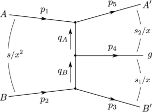
Figure 1: Schematic representation of the kinematics for the scattering process in eq. 1

We consider the scattering process

$$A^{\lambda_{A}}(p_{1})\;B^{\lambda_{B}}(p_{2})\to B^{\prime\lambda_{B^{\prime}}}(p_{3})\;g^{\lambda_{4}}(p_{4})\;A^{\prime\lambda_{A^{\prime}}}(p_{5})$$ (1)

where $A,A^{\prime},B,B^{\prime}$ are flavour indices and can either be $q(\bar{q})$ for quarks(anti-quarks) or $g$ for gluons, $p_{i}$ label the momenta of the scattering partons and $\lambda_{i}$ refer to their helicities. The MRK regime is defined as the configuration where the final-state partons are strongly ordered in rapidity, while their transverse components are commensurate and much smaller than the centre-of-mass energy $s_{12}=2p_{1}\cdot p_{2}$:

$$p_{1}^{+}\sim p_{5}^{+}\gg p_{4}^{+}\gg p_{3}^{+}\,,\quad p_{2}^{-}\sim p_{3}^{-}\gg p_{4}^{-}\gg p_{5}^{-}\,,\quad p_{4}^{\pm}\sim|{\bf q}_{A}|\sim|{\bf p}_{4}|\sim|{\bf q}_{B}|\,,$$ (2)

with $p_{1}^{+}=p_{2}^{-}=\sqrt{s_{12}}$, where we have introduced the light-cone coordinates in the notation $p^{\pm}=p^{0}\pm p^{z}$, ${\bf p}=\{p^{x},p^{y}\}$, and introduced the $t$-channel momenta

$$q_{A}=p_{5}-p_{1},\quad\quad\quad q_{B}=p_{4}+p_{5}-p_{1}=p_{2}-p_{3}\,,$$ (3)

see fig. 1. The helicity amplitudes for the process (1) can be described in terms of the five Mandelstam invariants

$$s_{12}=2p_{1}\cdot p_{2},\quad s_{23}=-2p_{2}\cdot p_{3},\quad s_{34}=2p_{3}\cdot p_{4},\quad s_{45}=2p_{4}\cdot p_{5},\quad s_{51}=-2p_{1}\cdot p_{5}\,,$$ (4)

and the parity-odd quantity

$$\mathrm{tr}_{5}\equiv{\rm Tr}[\gamma_{5}\not{p}_{1}\not{p}_{2}\not{p}_{3}\not{p}_{4}]=4i\epsilon_{\mu\nu\rho\sigma}p_{1}^{\mu}p_{2}^{\nu}p_{3}^{\rho}p_{4}^{\sigma},$$ (5)

where $\epsilon_{\mu\nu\rho\sigma}$ is the totally anti-symmetric Levi-Civita symbol. In MRK, they parametrically scale as

$$s_{12}\sim\mathrm{tr}_{5}\sim 1/x^{2},\quad s_{34}\sim s_{45}\sim 1/x,\quad s_{23}\sim s_{51}\sim 1,$$ (6)

with the scaling parameter $x\ll 1$. Also, in this limit

$$\mathrm{tr}^{2}_{5}=\Delta=s_{34}^{2}s_{45}^{2}(1-2\alpha-2\beta-2\alpha\beta+\alpha^{2}+\beta^{2})+\mathcal{O}\left(1/x^{3}\right),$$ (7)

where $\Delta=\mathrm{det}(G_{ij})$ and $G_{ij}=2p_{i}\cdot p_{j}$ with $i,j=1...4$ is the Gram matrix. This implies $\alpha=-s_{12}s_{23}/(s_{34}s_{45})$ and $\beta=-s_{12}s_{51}/(s_{34}s_{45})$.

To make the scaling eq. 6 manifest and simplify the quadratic relation (7), we follow ref. Caron-Huot:2020vlo and parametrise the kinematics in terms of $\mathcal{O}(1)$ invariants $\{s,s_{1},s_{2}\}$, a small dimensionless parameter $x$, and a complex variable $z$ such that

$$s_{12}=\frac{s}{x^{2}},\quad s_{23}=-\frac{s_{1}s_{2}}{s}z\bar{z},\quad s_{34}=\frac{s_{1}}{x},\quad s_{45}=\frac{s_{2}}{x},\quad s_{51}=-\frac{s_{1}s_{2}}{s}(1-z)(1-\bar{z})\,$$ (8)

with $\bar{z}=z^{*}$. Thanks to eq. 8, the parity odd invariant $\mathrm{tr}_{5}$ is then simply given by

$$\mathrm{tr}_{5}=\frac{s_{1}s_{2}}{x^{2}}(z-\bar{z})+\mathcal{O}(1/x)\,.$$ (9)

As we explicitly show in appendix A, it follows that the complex variable $z$ is related to the transverse momenta $q_{A,B}$ via

$$z=-\frac{q_{B}^{x}-iq_{B}^{y}}{|{\bf{p}}_{4}|},\quad\quad\quad 1-\bar{z}=\frac{q_{A}^{x}+iq_{A}^{y}}{|{\bf{p}}_{4}|}\,.$$ (10)

Let us stress that the role of the scaling parameter $x$ is effectively to ensure that the invariants $s$, $s_{1}$, and $s_{2}$ are of the same order, and that large-rapidity logarithms manifest themselves through the large quantity $\ln(x)$.

In the $2\to 3$ physical scattering region, the five Mandelstam invariants fulfil the following set of conditions Gehrmann:2018yef

$$s_{12}\geq s_{34},\quad\;s_{12}-s_{34}\geq s_{45},\quad\;s_{45}-s_{12}\leq s_{23}\leq 0,\quad\;s^{-}_{51}\leq s_{51}\leq s^{+}_{51},$$ (11)

with

$$s_{51}^{\pm}=\frac{1}{(s_{12}-s_{45})^{2}} \Big{[}s_{12}^{2}s_{23}+s_{34}s_{45}(s_{45}-s_{23})-s_{12}(s_{34}s_{45}+s_{23}s_{34}+s_{23}s_{45})$$

$$\pm\sqrt{s_{12}s_{23}s_{34}s_{45}(s_{12}+s_{23}-s_{45})(s_{34}+s_{45}-s_{12})}\,\Big{]}\,.$$ (12)

Figure 2: Representation of the $z$-complex plane in MRK in the strict $x\to 0$ limit. The shaded regions are forbidden whereas the lower and upper triangles are permitted.

Considering the $x\to 0$ behaviour of eq. 8, the first three conditions in eq. 11 are trivially satisfied. The last one, at fixed values of $s$, $s_{1}$ and $s_{2}$, defines an $x$-dependent exclusion region in the $z$-complex plane. In the strict $x\to 0$ limit, for any value of $s$ and $s_{1,2}$, this reduces simply to

$$|\mathrm{Im}(z)|\geq\sqrt{3}|{\rm Re}(z)|,$$ (13)

which is pictorially represented in fig. 2.

Finally we consider the scenario where the two light-cones are exchanged, i.e. we apply the $p_{1}\leftrightarrow p_{2}$ and $p_{3}\leftrightarrow p_{5}$ permutations. This allows one to investigate the $BA$ scattering channel starting from the $AB$ one of eq. 1. As for the invariants, see eqs. 8 and 5, this leads to

$$s_{1}\leftrightarrow s_{2}\quad\quad z\bar{z}\leftrightarrow(1-z)(1-\bar{z}),\quad\quad\mathrm{tr}_{5}\to\mathrm{tr}_{5},$$ (14)

where the last relation follows from the fact that we are considering an even permutation of momenta. In particular, since $\mathrm{tr}_{5}$ in MRK is given by eq. 9, this implies that $(z-\bar{z})\leftrightarrow(z-\bar{z})$. The latter, combined with the second relation in eq. 14 implies $z\leftrightarrow 1-\bar{z}$. Therefore, exchanging the two light-cones amounts simply to the transformations $s_{1}\leftrightarrow s_{2}$ and $z\leftrightarrow 1-\bar{z}$. Amplitudes where particles $A(B)$ and $A^{\prime}(B^{\prime})$ have the same flavour and helicity are then symmetric under this transformation.

2.2 Partonic channels, colour bases, and signature symmetry

In MRK, the only partonic configurations that contribute to eq. 1 at leading power in $x$ are those where both flavour and helicity are conserved along the large light-cone momenta lines, i.e.

$$A^{\lambda_{A}}(p_{1})B^{\lambda_{B}}(p_{2})\to B^{\lambda_{B}}(p_{3})g^{\lambda_{4}}(p_{4})A^{\lambda_{A}}(p_{5}).$$ (15)

To fix the notation, we define the scattering amplitude $\mathcal{A}$ in terms of the connected component of the $\mathcal{S}$-matrix as

$$\mathcal{S}_{\text{connected}}\equiv(2\pi)^{d}\delta^{d}(\textstyle\sum_{i}p_{i})(i\mathcal{A}).$$ (16)

We then write the ultra-violet (UV) renormalised scattering amplitude for the process (15) as

$$\mathcal{A}^{[AB]}_{\boldsymbol{\lambda}}=g_{s}^{3}\,2\sqrt{2}\,\Phi^{[AB]}_{\boldsymbol{\lambda}}\sum_{n}\mathcal{C}_{n}^{[AB]}\mathcal{B}_{n}^{[AB]}(\{s_{ij}\},\mathrm{tr}_{5};\boldsymbol{\lambda}),$$ (17)

where the pair $[AB]$ identifies the flavour configuration in the initial state, i.e. $[AB]$ can be $[gg],\,[qg]$ or $[qQ]$. In eq. 17 $g_{s}$ is the strong coupling, $\boldsymbol{\lambda}=\{\lambda_{B},\lambda_{4},\lambda_{A}\}$ are the final-state helicities, $\Phi^{[AB]}$ are helicity- and channel-dependent spinor factors, $\mathcal{C}_{n}$ are a set of colour tensors that span the colour space of the process, and $\mathcal{B}_{n}^{[AB]}$ are spinor- and colour-stripped scalar functions that contain the non-trivial perturbative information about the scattering amplitude. We expand them in terms of the strong coupling constant $\alpha_{s}$ as

$$\mathcal{B}_{n}^{[AB]}=\mathcal{B}_{n}^{[AB],(0)}+\left(\frac{\alpha_{s}}{4\pi}\right)\mathcal{B}_{n}^{[AB],(1)}+\left(\frac{\alpha_{s}}{4\pi}\right)^{2}\mathcal{B}_{n}^{[AB],(2)}+\mathcal{O}(\alpha_{s}^{3}),$$ (18)

where $\alpha_{s}=\alpha_{s}(\mu_{R})$ with $\mu_{R}$ the renormalisation scale. Since we are working with UV-renormalised amplitudes, infrared (IR) divergences manifest themselves as poles in the dimensional regulator $\epsilon=(4-d)/2$. We keep the $\epsilon$-dependence in $\mathcal{B}_{n}^{[AB],(l)}$ implicit. Also, note that throughout this paper we will use the superscript $(l)$ to denote the coefficient of $(\alpha_{s}\big{/}4\pi)^{l}$ in the perturbative expansion of the corresponding quantity (possibly ignoring an overall $g_{s}^{3}$ tree-level coupling factor, such that $\mathcal{A}^{[AB],(0)}$ denotes the tree-level amplitude).

We now discuss the various terms in eq. 15, starting with the spinor factors $\Phi^{[AB]}_{\boldsymbol{\lambda}}$. We choose them to be the tree-level (MHV) spinor amplitudes for the process eq. 15. Specifically, for the $\boldsymbol{\lambda}=\{+,+,+\}$ configuration, we then have

$$\Phi^{[gg]}_{\{+++\}} =\frac{\langle 12\rangle^{4}}{\langle 12\rangle\langle 23\rangle\langle 34\rangle\langle 45\rangle\langle 51\rangle},$$ (19)

$$\Phi^{[qg]}_{\{+++\}} =\frac{\langle 12\rangle^{3}\langle 25\rangle}{\langle 15\rangle\langle 52\rangle\langle 23\rangle\langle 34\rangle\langle 41\rangle},$$ (20)

$$\Phi^{[qQ]}_{\{+++\}} =\frac{\langle 12\rangle^{2}\langle 13\rangle\langle 25\rangle}{\langle 15\rangle\langle 52\rangle\langle 23\rangle\langle 34\rangle\langle 41\rangle}\,.$$ (21)

Results for other helicites (as well as for anti-quark channels) can be obtained from these via parity transformations, permutation of external momenta, and crossing symmetry. For a detailed discussion regarding our spinor products conventions in MRK we refer the reader to appendix A.

In order to discuss colour, we introduce the standard operators ${\bf T}_{i}$ defined as

$$\left(\mathbf{T}_{k}\right)^{c}_{ab}=if^{acb}\;\;\mathrm{if}\;k=g,\quad\;\left(\mathbf{T}_{k}\right)^{c}_{ij}=T^{c}_{ij}\;\;\mathrm{if}\;k=q,\quad\;\left(\mathbf{T}_{k}\right)^{c}_{ij}=-T^{c}_{ji}\;\;\mathrm{if}\;k=\bar{q}\,.$$ (22)

Here, both quarks and anti-quarks are taken to be outgoing, and $T^{c}_{ij}$ are generators of $SU(N_{c})$ in the fundamental representation satisfying $\mathrm{Tr}(T^{a}T^{b})=\delta^{ab}/2$. For future convenience, we also introduce the combinations

$${\bf T}^{\pm}_{15}={\bf T}_{1}\pm{\bf T}_{5},\quad\quad{\bf T}^{\pm}_{23}={\bf T}_{2}\pm{\bf T}_{3}.$$ (23)

As it will become apparent later on, in MRK it is natural to work in a colour basis $\mathcal{C}_{i}$ where each element is an eigenstate of both $({\bf T}^{+}_{15})^{2}$ and $({\bf T}^{+}_{23})^{2}$. We achieve this by choosing a basis of irreducible $SU(N_{c})$ representations in both the $s_{51}$ and $s_{23}$ channels. Each basis element can be labelled by a pair $(r_{1},r_{2})$, where $r_{1}$ and $r_{2}$ correspond to the representations in the $q_{A}\,(s_{51})$ and $q_{B}\,(s_{23})$ channels respectively. Specifically, we define $r_{1,2}$ through

$$R_{1}\otimes R_{5}=\oplus\,r_{1}\qquad R_{2}\otimes R_{3}=\oplus\,r_{2}\,,$$ (24)

with $R_{i}$ the representation of the $i$-th parton. The relevant decompositions we need are

$$8\otimes 8=\overbrace{0\oplus 1\oplus 8_{s}\oplus 27}^{\mathrm{symmetric}}\;\oplus\;\overbrace{8_{a}\oplus 10\oplus\overline{10}}^{\mathrm{anti-symmetric}},$$ (25)

for a gluon line, and

$$3\otimes\bar{3}=1\oplus 8\,,$$ (26)

for a quark line. The subscripts $a$ and $s$ in eq. 25 refer to the anti-symmetric and symmetric adjoint representations respectively, while “0” denotes an irreducible representation that is present in $SU(N_{c})$ for $N_{c}>3$, but not in $SU(3)$. We report more details about the colour decomposition in appendix B, including the explicit expressions for the $\mathcal{C}_{n}$ tensors (listed in tables 1 and 2). Here we only mention that we choose orthogonal bases, i.e.

$$\sum_{\mathrm{colour}}\left(\mathcal{C}^{[AB]}_{n}\right)^{\dagger}\mathcal{C}^{[AB]}_{m}=\mathcal{N}^{[AB]}_{m}\delta_{mn}\,.$$ (27)

Also, we note that in the gluon case this colour basis naturally splits into tensors which have well-defined symmetry properties under exchange of the colour labels for the two external gluons of the relevant channel, as shown by the braces in eq. 25.

Finally, in MRK it is also convenient to work with signature eigenstates, i.e. states which have well-defined symmetry properties under the exchange of initial and final states. Indeed, only one signature eigenstate captures the leading behaviour of the cross section in the high-energy limit (see e.g. Caron-Huot:2017fxr ). We then define the following operations on the scalar functions $\mathcal{B}$ 

$$\mathcal{B}_{n}^{[AB],(l)}(s_{12},s_{23},s_{34},s_{45},s_{51},\mathrm{tr}_{5};\boldsymbol{\lambda})\big{|}_{1\leftrightarrow 5}=\mathcal{B}_{n}^{[AB],(l)}(s_{52},s_{23},s_{34},s_{41},s_{51},-\mathrm{tr}_{5};\boldsymbol{\lambda}),$$

$$\mathcal{B}_{n}^{[AB],(l)}(s_{12},s_{23},s_{34},s_{45},s_{51},\mathrm{tr}_{5};\boldsymbol{\lambda})\big{|}_{2\leftrightarrow 3}=\mathcal{B}_{n}^{[AB],(l)}(s_{13},s_{23},s_{24},s_{45},s_{51},-\mathrm{tr}_{5};\boldsymbol{\lambda}),$$ (28)

$$\mathcal{B}_{n}^{[AB],(l)}(s_{12},s_{23},s_{34},s_{45},s_{51},\mathrm{tr}_{5};\boldsymbol{\lambda})\big{|}_{\begin{subarray}{c}1\leftrightarrow 5\\ 2\leftrightarrow 3\end{subarray}}=\mathcal{B}_{n}^{[AB],(l)}(s_{53},s_{23},s_{24},s_{41},s_{51},+\mathrm{tr}_{5};\boldsymbol{\lambda}).$$

Crucially, these transformations exchange positive with negative Mandelstam invariants and thus require a non-trivial analytic continuation of the amplitudes. To achieve the latter, we exploit the explicit expressions of the ensuing transcendental functions in all 5! kinematic regions of $2\to 3$ scattering Chicherin:2020oor and follow the procedure described in refs. Agarwal:2021vdh ; Agarwal:2023suw to cross those functions from a given region to another one.

We define the following eigenstates 

$$\mathcal{B}_{n}^{[AB],(l),(\sigma_{1},\sigma_{2})}=\frac{1}{4}\Big{[} \mathcal{B}_{n}^{[AB],(l)}-\sigma_{1}\mathcal{B}_{n}^{[AB],(l)}\big{|}_{1\leftrightarrow 5}\,\,-$$ (29)

$$\sigma_{2}\mathcal{B}_{n}^{[AB],(l)}\big{|}_{2\leftrightarrow 3}\,\,+\sigma_{1}\sigma_{2}\mathcal{B}_{n}^{[AB],(l)}\big{|}_{\begin{subarray}{c}1\leftrightarrow 5\\ 2\leftrightarrow 3\end{subarray}}\Big{]}\,.$$

In the same spirit, we introduce the definite-signature colour operators

$$\boldsymbol{\mathcal{T}}_{\sigma_{1}\sigma_{2}}={\bf T}_{15}^{\sigma_{1}}\cdot{\bf T}_{23}^{\sigma_{2}}\,,$$ (30)

and note that all our colour basis elements are by construction eigenstates of $\boldsymbol{\mathcal{T}}_{++}$ since

$$\boldsymbol{\mathcal{T}}_{++}=\frac{1}{2}\left({{\bf T}_{4}}^{2}-({\bf T}^{+}_{15})^{2}-({\bf T}^{+}_{23})^{2}\right)\,.$$ (31)

We point out that thanks to Bose statistics the (anti)symmetrisation over a gluon line is equivalent to (anti)symmetrising its colour indices. Therefore, selecting a signature eigenstate corresponds to selecting a symmetric or antisymmetric representation in the $8\otimes 8$ decomposition, see eq. 25. The same is not true in general for quarks.

We conclude this section by stressing that all the manipulations and definitions described above do not require the MRK limit. However, they make the study of this kinematic configuration particularly transparent. Indeed, as we will review later on, in the MRK regime the amplitude naturally organises into contributions coming from $t$-channel exchanges of effective degrees of freedom – reggeons – which have well-defined colour and signature symmetry. Writing the amplitude in the way described in this section helps uncover such a structure.

2.3 MRK expansion of the full scattering amplitudes

Having set our notation, we can now expand in MRK the full two-loop scattering amplitudes that some of us computed Agarwal:2023suw . To do so, we first note that the spinor factors defined in eq. 19 capture the leading-power multi-Regge behaviour, $\Phi^{[AB]}_{\boldsymbol{\lambda}}\sim 1/x^{2}$. This implies that at leading power

$$\mathcal{B}^{[AB]}_{n}\sim{\rm const}+\mathcal{O}(x).$$ (32)

The scattering amplitudes are schematically written as Agarwal:2023suw

$$\mathcal{B}^{[AB]}_{n}=\sum\left[R_{a,k}(\{s_{ij}\};\epsilon_{5})+\mathrm{tr}_{5}R_{b,k}(\{s_{ij}\};\epsilon_{5})\right]\times f_{k}(\{W\}),$$ (33)

where $R$ are rational functions of the external kinematics, while $f_{k}$ are transcendental functions, referred to as pentagon functions Gehrmann:2018yef ; Abreu:2018aqd ; Chicherin:2018old ; Chicherin:2020oor . The latter are pure functions of uniform transcendentality, that depend on the 31 letters of the pentagon alphabet $\{W\}$ Abreu:2018aqd ; Chicherin:2018old ; Chicherin:2020oor . Finally, we introduced a further dependence on $\epsilon_{5}$, which is related to the Gram determinant via $\epsilon_{5}=i\sqrt{|\Delta|}$. Note that for $\epsilon_{5}$ we adopt the same convention of ref. Chicherin:2020oor , i.e. we define it with a positive imaginary part. This implies $\epsilon_{5}=+i|{\rm tr}_{5}|$, and therefore in MRK

$$\epsilon_{5}\simeq\frac{s_{1}s_{2}}{x^{2}}\times\begin{cases}\left(z-\bar{z}\right)\quad\mathrm{if}\;\mathrm{Im}(z)>0,\\ \left(\bar{z}-z\right)\quad\mathrm{if}\;\mathrm{Im}(z)<0\,.\end{cases}$$ (34)

The expansion of the rational functions is straightforward. However, due to their large number and sheer size, this task can be computationally intensive. For this purpose we use the computer algebra program FORM Vermaseren:2000nd ; Ruijl:2017dtg . Furthermore, when the amplitude is expanded in terms of the pentagon functions, the rational coefficients $R$ develop spurious higher poles in $x=0$. To obtain the leading MRK behaviour of the amplitude, the transcendental functions then need to be expanded around $x=0$ beyond leading power. In particular, we require the expansion of $f_{k}$ up to second order in $x$. Fortunately, the pentagon functions are written as iterated integrals, which makes such an expansion straightforward.

Before describing how we proceed with the expansion, we comment on eq. 34. As discussed in detail in ref. Caron-Huot:2020vlo , amplitudes in MRK are non real analytic when crossing the $\epsilon_{5}=0$ ($\mathrm{Im}(z)=0$) hyper-surface. This would require to analytically continue the ensuing results from the upper to the lower half of the complex plane, or vice-versa. Similarly to ref. Caron-Huot:2020vlo , we prefer instead to expand the pentagon functions separately in both regions. The approach is indeed identical, and care just needs to be taken when fixing an initial boundary condition.

Leading-power expansion

We now discuss how to obtain the leading-power MRK behaviour of a generic weight-$w$ pentagon function $f_{i}^{(w)}(\{W\})$ of ref. Chicherin:2020oor . By construction, those obey a differential equation of the form

$$\mathrm{d}f_{i}^{(w)}=\sum_{k=1}^{31}{\mathrm{d}}\ln(W_{k})\times\bigg{[}\mathrm{linear~{}combinations~{}of~{}lower~{}weight~{}}f_{j}^{(w^{\prime})}\bigg{]}.$$ (35)

Crucially, $a)$ the bracket on the r.h.s. involve linear combinations of $f^{(w^{\prime})}_{j}$ whose coefficients are rational numbers, and $b)$ the total transcendental weight of each term in the bracket is exactly $w-1$. Assuming that the weight-$(w-1)$ functions in the MRK expansion are known, one can then readily obtain the desired result at weight $w$ by expanding the pentagon alphabet $\{W\}$ at leading power in $x$ in the differential equation in eq. 35, and integrate it back. Although all of this is quite standard, we now provide additional details on the procedure for the sake of completeness.

First, we point out that the pentagon alphabet drastically simplifies in the MRK limit. Indeed, the 31 $\mathrm{d}\ln(W_{k})$ can all be expressed in terms of 12 $\mathrm{d}\ln v_{i}$, where the letters $v_{i}$ are Caron-Huot:2020vlo

$$\{x\},\;\;\;\left\{\frac{s_{1}s_{2}}{s}\right\},\;\;\;\{s_{1},s_{2},s_{1}-s_{2},s_{1}+s_{2}\},\;\;\;\{z,\bar{z},1-z,1-\bar{z},1-z-\bar{z},z-\bar{z}\}\,.$$ (36)

A few comments on the alphabet eq. 36 are in order. First, note the separation between longitudinal ($s_{i}$) and transverse ($z,\bar{z})$ variables. Second, this alphabet implies that all our results can be expressed in terms of $\ln(x)$, and 2dHPLs Gehrmann:2000zt ; Gehrmann:2001ck ; Gehrmann:2001jv of $\{s,s_{1},s_{2}\}$ and of $\{z,\bar{z}\}$. Given this, obtaining the desired result is straightforward. We assume that the result at weight $w-1$ is both known and expressed in terms of a minimal basis of 2dHPLs $\{G^{(w-1)}\}$. Then, all one has to do is

• write the most general weight$-w$ ansatz starting from a minimal 2dHPLs basis $\{G^{(w)}\}$ (and products of lower-weight 2dHPLs and constants such that the total weight is $w$) ;

• take the differential of the ansatz, and express it in terms of $\{G^{(w-1)}\}$;

• match this result against eq. 35 to fix all the unknown coefficients;

• fix a missing overall constant by computing the result in a specific kinematic point (which must be in the exact MRK limit).

We now provide some extra detail on the practical implementation of this procedure. First, we note that in principle one could read off the differential of the pentagon functions directly from their iterated form given in ref. Chicherin:2020oor . However, this would require dealing with a very large number of different weight-3 functions. We then decided to re-derive the differential equations in eq. 35 starting from the canonical basis of one- and two-loop five-point master integrals provided in ref. Chicherin:2020oor , exploiting their expressions in terms of pentagon functions. To do so, we used the programs Reduze Studerus:2009ye ; vonManteuffel:2012np to obtain the derivatives w.r.t. the $s_{ij}$, and Kira Klappert:2019emp ; Klappert:2020nbg to perform the necessary integration-by-parts reduction to master integrals. We then reconstruct the differential equations for the canonical master integrals $G_{i}$ in the form

$$\mathrm{d}G_{i}=\epsilon\,\sum_{jk}A_{ijk}{\mathrm{d}}\ln(W_{j})\;G_{k}$$ (37)

by numerically fitting the coefficients $A_{ijk}$. Finally, substituting the solutions for the master integrals, expressed in terms of pentagon functions $f^{(w)}_{i}$ Chicherin:2020oor , into eq. 37 and collecting the different powers of $\epsilon$ on the l.h.s. and r.h.s. , we obtain the differential equations of eq. 35.

We also note that the alphabet  (36) leads to the following spurious singularities:

• $s_{1}=\pm s_{2}$, corresponding to $s_{34}=\pm s_{45}$,

• $z=\bar{z}$, corresponding to $\epsilon_{5}=0$,

• $1-z-\bar{z}=0\Leftrightarrow{\rm Re}(z)=1/2$, corresponding to $s_{23}=s_{51}$.

Although they cannot be present in the physical result, they appear in individual pentagon functions and the fate of their cancellation is different. Indeed, the $s_{1}=\pm s_{2}$ singularity explicitly drops out from the UV-renormalised amplitudes. Functions involving the $z-\bar{z}$ letter are present in the UV-renormalised amplitudes, but drop out from four-dimensional finite remainders (see section 2.4). Finally, ${\rm Re}(z)=1/2$ remains as a spurious singularity if the amplitude is expressed in terms of 2dHPLs, or in terms of the single-valued polylogarithms described in section 2.4.

To conclude our discussion about the leading-power expansion of the pentagon functions, we now illustrate how we obtained a boundary condition in MRK. By construction, in the point $X_{0}=\{s_{12},s_{23},s_{34},s_{45},s_{51}\}=\{3,-1,1,1,-1\}$, the pentagon functions either vanish or can be expressed in terms of few simple transcendental constants Chicherin:2020oor . We point out that in principle both $\mathrm{Im}(z)>0$ and $\mathrm{Im}(z)<0$ are allowed when translating this point from the $s_{ij}$ to the complex variables of eq. 8. We thus solve the system of differential equations in both the upper and lower halves of the complex plane choosing $\mathrm{Im}(z)$ accordingly in the boundary value. We then consider the family of kinematic points $Y=\{3/x^{2},-1,1/x,1/x,-1\}$ and use the differential equation in $x$ to transport the $X_{0}$ boundary ($x=1$) to the $x=0$ MRK point. The differential equation in $x$ contains square roots, but they are easily rationalisable, allowing us to obtain an analytic result.

We express the result in terms of Goncharov polylogarithms, that we numerically evaluate with very high precision using GiNaC Bauer:2000cp in the boundary points $x=1$ and $x=0$. We then use the PSLQ algorithm Ferguson:PSLQ to express the final boundary points for the expanded pentagon functions in terms of simple transcendental constants. A complete set of such constants was already discussed in ref. Caron-Huot:2020vlo (see tab. 2 therein), so we do not repeat them here. Throughout the whole procedure we made use of the program PolyLogTools Duhr:2019tlz to deal with the differential equations and for manipulations involving the Goncharov polylogarithms.

Sub-leading-power expansion

If the leading-power expansion of the pentagon functions is known, obtaining higher powers is straightforward. Indeed, all one needs to do is to write a generalised power series in $x$ of the form

$$f^{(w)}_{i}=\sum_{\ell=0}\sum_{m=0}^{w}x^{\ell}\ln^{m}(x)g^{(w)}_{i,\ell m}\left(\{s,s_{1},s_{2}\},\{z,\bar{z}\}\right)\,,$$ (38)

insert it in the differential equation (35), expand the $\mathrm{d}\ln\left(W_{k}\right)$ forms accordingly up to desired power in $x$, and solve the differential equation term by term in $x$ and $\ln x$. Since the resulting differential equation has the schematic form

$${\mathrm{d}}f_{i}^{(w)}=\left[\frac{A_{ij}^{(-1)}}{x}+A_{ij}^{(0)}+x\,A_{ij}^{(1)}+...\right]f_{i}^{(w)},$$ (39)

it is easy to see that beyond leading power, at any transcendental weight $w$ and power in $x$, the problem is turned into solving a linear system of equations for the coefficient functions $g^{(w)}_{i,\ell m}$. For this purpose, we make use of the program FiniteFlow Peraro:2019svx , that allows us to efficiently reach high powers in $x$. In the ancillary files provided alongside this publication, we present expansions of all the pentagon functions in MRK up to $\mathcal{O}(x^{4})$. Following the discussion on the non-real analyticity property of the pentagon functions in crossing $\mathrm{Im}(z)=0$, we provide results in both the lower and upper halves of the complex $z$ plane.

We checked the correctness of such expansions by comparing the results in a dozen of kinematic points against a numerical evaluation of the complete pentagon functions in quadruple precision Chicherin:2020oor for small-$x$ values. We found excellent agreement within the expected accuracy of the expansion.

2.4 IR subtraction and finite remainders

The procedures described in the previous sections lead to UV-renormalised amplitudes in MRK which still contain (universal) IR singularities. The factorisation of IR divergences in scattering amplitudes allows us to define a finite remainder (or hard amplitude), which encodes the non-trivial physical information. As we noted in the previous section, its structure is simpler than the one of the IR-divergent amplitude.

The IR structure of two-loop QCD amplitudes is well known Catani:1998bh ; Aybat:2006mz ; Becher:2009qa ; Gardi:2009zv . Here we follow ref. Becher:2009qa and define ($\overline{\rm MS}$) finite remainders $\mathbf{\mathcal{H}}^{[AB]}_{n}$ as

$$\boldsymbol{\mathcal{H}}^{[AB]}=\lim_{\epsilon\to 0}\,\mathbf{Z}_{IR}^{-1}\,\boldsymbol{\mathcal{B}}^{[AB]},$$ (40)

where we used the vector notation $\boldsymbol{\mathcal{H}}^{[AB]}=\big{\{}\mathcal{H}^{[AB]}_{n}\big{\}}$, $\mathbf{Z}_{IR}$ is a matrix in colour space and the perturbative expansion of $\mathbf{\mathcal{H}}^{[AB]}_{n}$ is defined in the same way as in eq. 18. From now on, we will drop the $[AB]$ superscript whenever this is not ambiguous to avoid cluttering the notation.

Up to two loops, the $\mathbf{Z}_{IR}$ matrix can be written as

$$\mathbf{Z}_{IR}(\epsilon,\{p\},\mu)=\exp\left[\int^{\infty}_{\mu}\frac{\mathrm{d}\mu^{\prime}}{\mu^{\prime}}{\bf\Gamma}_{IR}(\{p\},\mu^{\prime})\right]\;,$$ (41)

where $\mu$ is an arbitrary IR scale, and

$${\bf\Gamma}_{IR}(\{p\},\mu) =\gamma_{K}(\alpha_{s})\sum_{\begin{subarray}{c}i,j=1\\ i>j\end{subarray}}^{5}\mathbf{T}_{i}\cdot\mathbf{T}_{j}\ln\left(\frac{\mu^{2}}{-s_{ij}-i\delta}\right)+\sum_{i=1}^{5}\gamma_{i}(\alpha_{s})\,.$$ (42)

In the equation above, $\alpha_{s}=\alpha_{s}(\mu)$, $\gamma_{K}$ is the QCD cusp anomalous dimension Korchemsky:1987wg ; Moch:2004pa and $\gamma_{i}$ are the collinear anomalous dimensions Ravindran:2004mb ; Moch:2005id ; Moch:2005tm . They are given explicitly in appendix C up to the relevant perturbative order. In MRK, the soft anomalous dimension eq. 42 can be written as

$${\bf\Gamma}_{IR}= \frac{\gamma_{K}}{2}\bigg{\{}\left({\bf T}^{15}_{+}\right)^{2}\left[\ln\frac{s_{45}}{-s_{51}}+\ln\frac{s_{45}}{{\bf p}_{4}^{2}}-i\pi\right]+\left({\bf T}^{23}_{+}\right)^{2}\left[\ln\frac{s_{34}}{-s_{23}}+\ln\frac{s_{34}}{{\bf p}_{4}^{2}}-i\pi\right]$$ (43)

$$- 2\,\mathcal{C}_{A}\ln\frac{\mu^{2}}{-s_{51}}-2\,\mathcal{C}_{B}\ln\frac{\mu^{2}}{-s_{23}}-\mathcal{C}_{g}\ln\frac{\mu^{2}}{{\bf p}_{4}^{2}}+i\pi\left[\boldsymbol{\mathcal{T}}_{+-}+\boldsymbol{\mathcal{T}}_{-+}+\boldsymbol{\mathcal{T}}_{--}-\boldsymbol{\mathcal{T}}_{++}\right]\bigg{\}}$$

$$+ 2\gamma_{A}+2\gamma_{B}+\gamma_{g},$$

where we assume that the pairs of particles $(1,5)$ and $(2,3)$ have the same flavour within each pair, and where $\mathcal{C}_{A(B)}$ is the quadratic Casimir of the colour representation of particle $A(B)$, i.e. $\mathcal{C}_{g}=C_{A}$ and $\mathcal{C}_{q}=\mathcal{C}_{\bar{q}}=C_{F}$. Note that, in our colour basis, the soft anomalous dimension is diagonal except for the signature-changing term

$$\frac{\gamma_{K}}{2}\times i\pi\left[\boldsymbol{\mathcal{T}}_{+-}+\boldsymbol{\mathcal{T}}_{-+}+\boldsymbol{\mathcal{T}}_{--}\right].$$ (44)

As we will discuss in section 4.3, the soft anomalous dimension (43) can be organised in a form that makes MRK factorisation manifest. For now, we limit ourselves to discussing the properties of the finite remainders defined through eq. 40. For a given signature, we write them as

$$\boldsymbol{\mathcal{H}}^{(l),(\sigma_{1},\sigma_{2})}=\sum_{k=0}^{l}\boldsymbol{\mathcal{H}}^{(l),(\sigma_{1},\sigma_{2})}_{(k)}L^{k},$$ (45)

where for convenience we have expanded in $L=-\ln(x)-i\pi/2$. We will justify this form in section 3. At LO, only the odd-odd signature featuring a double antisymmetric colour-octet exchange is present in MRK. Specifically, within our choice of spinor factors $\Phi_{\boldsymbol{\lambda}}$ we have

$$\mathcal{H}^{[gg],(0),(--)}_{(8_{a},8_{a})}=\mathcal{H}^{[qg],(0),(--)}_{(8,8_{a})_{a}}=\mathcal{H}^{[qQ],(0),(--)}_{(8,8)_{a}}=1+\mathcal{O}(x),$$ (46)

while all other contributions are power suppressed. The subscripts in the finite remainders $\mathcal{H}$ label the colour-basis element, see tables 1 and 2 for details.

As we will summarise later on, this corresponds to single-reggeon exchanges in both the $s_{51}$ and $s_{23}$ channels.

Basis of transcendental functions

Beyond leading order (LO), we find that the finite remainders can be expressed entirely in terms of simple logarithms of longitudinal variables and single-valued functions of $z$ and $\bar{z}$. The relevant basis has already been discussed in ref. Caron-Huot:2020vlo , thus we borrow it from there. The one-loop finite remainder can be written in terms of

$$\ln\left(\frac{\mu^{2}}{{\bf p}_{4}^{2}}\right),\quad\quad\ln\left(\frac{\mu^{2}}{s_{1}}\right),\quad\quad\ln\left(\frac{\mu^{2}}{s_{2}}\right),\quad\quad$$ (47)

plus the following weight-one single-valued functions Caron-Huot:2020vlo

$$\begin{gathered}g_{1,4}=\ln(z\bar{z}),\quad g_{1,5}=\ln\big{(}(1-z)(1-\bar{z})\big{)},\\ g_{1,6}=\ln(z)-\ln(\bar{z}),\quad g_{1,7}=\ln(1-z)-\ln(1-\bar{z}),\end{gathered}$$ (48)

and, at weight two,

$$g_{2,1} =D_{2}(z,\bar{z}),$$ (49)

$$g_{2,2} =\mathrm{Li}_{2}(z)+\mathrm{Li}_{2}(\bar{z}),$$ (50)

$$g_{2,3} =\mathrm{Li}_{2}\left(\frac{z}{1-\bar{z}}\right)+\mathrm{Li}_{2}\left(\frac{\bar{z}}{1-z}\right)+\left(g_{1,4}-g_{1,5}\right)\ln(|1-z-\bar{z}|)$$

$$+i\pi\left(g_{1,6}+g_{1,7}\right){\rm sgn}[{\rm Im}(z)]\Theta\left({\rm Re}(z)-\frac{1}{2}\right),$$ (51)

where $\Theta$ is the Heaviside step function, and $D_{2}(z,\bar{z})$ is the Bloch-Wigner dilogarithm defined as

$$D_{2}(z,\bar{z})=\mathrm{Li}_{2}(z)-\mathrm{Li}_{2}(\bar{z})+\frac{\ln(z\bar{z})}{2}\left(\ln(1-z)-\ln(1-\bar{z})\right),$$ (52)

which enjoys the property $D_{2}(z,\bar{z})=D_{2}(1-\bar{z},1-z)$.

For the two-loop finite remainder, weight 3 and 4 functions are also required. In ref. Caron-Huot:2020vlo it was observed that in $\mathcal{N}=4$ sYM the weight-four term can always be written in terms of product of functions of lower weight. We find that the same property also holds in QCD. More explicitly, at weight four there are only products of simple logarithms and $D_{2}(z,\bar{z})$ multiplied by $\zeta_{2}$. To write the two-loop finite remainder, we then only need to supplement eqs. 48 and 49 with the weight-three functions Caron-Huot:2020vlo

$$g_{3,1} =D_{3}(z,\bar{z}),$$ (53)

$$g_{3,2} =D_{3}(1-z,1-\bar{z}),$$ (54)

$$g_{3,3} =\mathrm{Li}_{3}(z)-\mathrm{Li}_{3}(\bar{z}),$$ (55)

$$g_{3,4} =\mathrm{Li}_{3}(1-z)-\mathrm{Li}_{3}(1-\bar{z})$$ (56)

$$g_{3,5} =\mathrm{Li}_{3}\left(\frac{z\bar{z}}{(1-z)(1-\bar{z})}\right)+\frac{1}{2}\ln(1-z-\bar{z})\ln^{2}\left(\frac{z\bar{z}}{(1-z)(1-\bar{z})}\right),$$ (57)

$$g_{3,6} =2\,\mathrm{Li}_{3}\left(\frac{z}{1-\bar{z}}\right)-2\mathrm{Li}_{3}\left(\frac{\bar{z}}{1-z}\right)-\ln\left(\frac{z\bar{z}}{(1-z)(1-\bar{z})}\right)D_{2}\left(\frac{z}{1-\bar{z}},\frac{\bar{z}}{1-z}\right)$$

$$+\frac{i\pi}{2}\left[(g_{1,4}-g_{1,5})^{2}+(g_{1,6}+g_{1,7})^{2}\right]{\rm sgn}[{\rm Im}(z)]\,\Theta\left({\rm Re}(z)-\frac{1}{2}\right),$$ (58)

$$g_{3,9} =\mathrm{Li}_{3}\left(\frac{1-z-\bar{z}}{(1-z)(1-\bar{z})}\right),$$ (59)

where we introduced

$$D_{3}(z,\bar{z})=\mathrm{Li}_{3}(z)+\mathrm{Li}_{3}(\bar{z})-\frac{1}{2}\ln(z\bar{z})\big{(}\mathrm{Li}_{2}(z)+\mathrm{Li}_{2}(\bar{z})\big{)}-\frac{1}{4}\ln^{2}(z\bar{z})\ln\left((1-z)(1-\bar{z})\right).$$ (60)

In passing, we note that our QCD results share the same set of single-valued functions of the $\mathcal{N}=4$ sYM results, except for $g_{2,3}$ and $g_{3,9}$ which instead appear in $\mathcal{N}=8$ supergravity Caron-Huot:2020vlo .

As discussed at the end of section 2.1, the $s_{1}\leftrightarrow s_{2}$ and $z\leftrightarrow 1-\bar{z}$ transformations corresponds to interchanging the two light cones. We thus find it convenient to introduce a basis of functions with definite symmetry under these transformations, either even or odd. At weight one and two we define,

$$\begin{gathered}h_{1,1}=g_{1,4}+g_{1,5},\quad h_{1,2}=g_{1,4}-g_{1,5},\quad h_{1,3}=g_{1,6}+g_{1,7},\quad h_{1,4}=g_{1,6}-g_{1,7},\quad\\ h_{2,1}=g_{2,1}\quad\\ h_{2,2}=g_{2,2}+\frac{h^{2}_{1,1}-h^{2}_{1,2}+h^{2}_{1,3}-h^{2}_{1,4}}{16}-\zeta_{2},\quad h_{2,3}=g_{2,3}+\frac{h_{1,2}^{2}+h_{1,3}^{2}}{8}-2\zeta_{2}\,,\end{gathered}$$ (61)

and at weight three,

$$\begin{gathered}h_{3,1}=g_{3,1}+g_{3,2},\quad h_{3,2}=g_{3,1}-g_{3,2},\quad h_{3,3}=g_{3,3}+g_{3,4},\quad h_{3,4}=g_{3,3}-g_{3,4},\\ h_{3,5}=g_{3,5}+\frac{h^{3}_{1,2}}{12}-\zeta_{2}\,h_{1,2},\quad h_{3,6}=g_{3,9}+\frac{g_{3,5}}{2}-\frac{h_{1,1}h^{2}_{1,2}}{8}-\frac{\zeta_{3}}{2},\quad\\ h_{3,7}=g_{3,6}+\frac{h^{3}_{1,3}}{24}+\frac{h^{2}_{1,2}h_{1,3}}{8}-2\zeta_{2}\,h_{1,3}\,.\end{gathered}$$ (62)

Given that the $h_{w,i}$ functions are built in terms of the $g_{w,j}$ ones, they also are single valued. In particular, the functions $h_{1,1}$, $h_{1,4}$, $h_{2,1}$, $h_{3,1}$, $h_{3,4}$, $h_{3,5}$ and $h_{3,7}$ are symmetric under $z\leftrightarrow 1-\bar{z}$, while the other ones are odd. Furthermore, they are also either even or odd under the transformation $z\to\bar{z}$, a property inherited from the $g_{i,j}$ functions above.

Final results

The complete results for the finite remainders for all partonic channels can be found in the ancillary files. Here we only report a few examples to illustrate their simplicity.

We focus on $gg$ scattering, and consider antisymmetric colour-octet exchanges in both the $s_{51}$ and $s_{23}$ channels. As explained in section 2.2, for gluon scattering this automatically selects the $(--)$ signature component. This amplitude is symmetric under the exchange of the plus and minus light-cones, thus any even(odd) function $h_{w,i}$ needs to be paired to an even(odd) rational function of $(z,\bar{z})$. Up to two loops we find only six independent rational functions,

$$\begin{gathered}r_{1}=\frac{z^{3}+(1-\bar{z})^{3}}{(1-z-\bar{z})^{3}},\quad r_{2}=\frac{z(1-\bar{z})}{(1-z-\bar{z})^{2}}\left(\frac{1}{1-z}+\frac{1}{\bar{z}}\right),\quad r_{3}=\frac{1+z-\bar{z}}{1-z-\bar{z}},\\ r_{4}=\frac{z(1-\bar{z})}{(1-z)\bar{z}},\quad r_{5}=\frac{z(1-\bar{z})}{(1-z-\bar{z})^{2}},\quad r_{6}=\frac{z(1-\bar{z})(z-\bar{z})}{\bar{z}(1-z)(1-z-\bar{z})}\,,\end{gathered}$$ (63)

with $r_{1}$, $r_{3}$ and $r_{6}$ odd, and $r_{2}$, $r_{4}$ and $r_{5}$ even. For the centrally-emitted gluon with positive helicity, at one loop we have

$$\mathcal{H}_{(8_{a},8_{a})}^{[gg],(1),(--)} =N_{c}\Bigg{[}\frac{17\pi^{2}}{12}-2h_{1,1}L-\frac{h^{2}_{1,2}}{2}+\left(\ln\left(\frac{s_{1}s_{2}}{s^{2}}\right)-\frac{i\pi}{2}\right)h_{1,1}-\ln\left(\frac{s_{1}}{s_{2}}\right)h_{1,2}\Bigg{]}$$

$$+\left(N_{c}-n_{f}\right)\left[\frac{h_{1,1}-r_{1}h_{1,2}-r_{2}}{3}\right]+\frac{3}{2}N_{c}\left(h_{1,1}-r_{3}h_{1,2}\right)-\frac{\gamma^{(2)}_{K}}{4},$$ (64)

where the explicit expression of the cusp anomalous dimension coefficient $\gamma^{(2)}_{K}$ is given in eq. 214. The equivalent result for the negative helicity case can be obtained by the simple replacement $z\leftrightarrow\bar{z}$. For the same helicity configuration, at two loops we find

$$\mathcal{H}_{(8_{a},8_{a})}^{[gg],(2),(--)}=N_{c}^{2}\Bigg{[}2L^{2}h_{1,1}^{2}+L\bigg{(}-2\log\left(\frac{s_{1}s_{2}}{s^{2}}\right)h_{1,1}^{2}+i\pi h_{1,1}^{2}+h_{1,2}^{2}h_{1,1}-17\zeta_{2}h_{1,1}$$

$$\quad\quad+2\log\left(\frac{s_{1}}{s_{2}}\right)h_{1,2}h_{1,1}+3r_{3}h_{1,2}h_{1,1}-4\zeta_{3}+\frac{232}{9}\bigg{)}+\frac{h_{1,2}^{4}}{8}+\frac{1}{2}\log^{2}\left(\frac{s_{1}}{s_{2}}\right)h_{1,2}^{2}$$

$$\quad\quad-\frac{9}{2}h_{2,2}h_{1,2}+\frac{1}{2}\log^{2}\left(\frac{s_{1}s_{2}}{s^{2}}\right)h_{1,1}^{2}+\frac{1677\zeta_{4}}{16}-\zeta_{3}h_{1,1}+\frac{58h_{1,1}}{9}-3\big{(}r_{2}+r_{1}h_{1,2}\big{)}$$

$$\quad\quad+\log\left(\frac{s_{1}}{s_{2}}\right)\bigg{(}\frac{1}{2}\big{(}3r_{3}+h_{1,2}-3\big{)}h_{1,2}^{2}-\frac{17}{2}\zeta_{2}h_{1,2}-\log\left(\frac{s_{1}s_{2}}{s^{2}}\right)h_{1,1}h_{1,2}$$

$$\quad\quad+\frac{i\pi}{2}h_{1,1}h_{1,2}\bigg{)}-\frac{\zeta_{2}}{4}\bigg{(}6h_{1,1}^{2}+23h_{1,2}^{2}+\frac{209}{3}+39r_{3}h_{1,2}\bigg{)}$$

$$\quad\quad+\log\left(\frac{s_{1}s_{2}}{s^{2}}\right)\bigg{(}-\frac{1}{2}i\pi h_{1,1}^{2}+\frac{17}{2}\zeta_{2}h_{1,1}-\frac{3}{2}r_{3}h_{1,2}h_{1,1}+2\zeta_{3}-\frac{1}{18}\big{(}9h_{1,1}h_{1,2}^{2}+232\big{)}\bigg{)}$$

$$\quad\quad+i\pi\bigg{(}\frac{1}{4}h_{1,1}h_{1,2}^{2}-\frac{\zeta_{3}}{2}-\frac{17}{4}\zeta_{2}h_{1,1}+\frac{3}{16}r_{3}\big{(}h_{1,1}h_{1,2}-h_{1,3}h_{1,4}-8h_{2,2}+8h_{2,3}\big{)}+\frac{29}{9}\bigg{)}$$

$$\quad\quad-\frac{3}{16}r_{3}\big{(}2h_{1,2}^{3}+\big{(}3h_{1,1}^{2}-16\big{)}h_{1,2}+h_{1,1}\big{(}h_{1,3}h_{1,4}+8h_{2,2}-8h_{2,3}\big{)}+64h_{3,6}\big{)}-\frac{1717}{54}\Bigg{]}$$

$$\quad\quad+N_{c}\big{(}N_{c}-N_{f}\big{)}\Bigg{[}+\frac{2}{27}L\big{(}9h_{1,1}\big{(}r_{2}+r_{1}h_{1,2}\big{)}+56\big{)}+\frac{1}{3}\log\left(\frac{s_{1}}{s_{2}}\right)h_{1,2}\big{(}r_{2}+\big{(}r_{1}-1\big{)}h_{1,2}\big{)}$$

$$\quad\quad+\frac{1}{27}\log\left(\frac{s_{1}s_{2}}{s^{2}}\right)\big{(}-9h_{1,1}\big{(}r_{2}+r_{1}h_{1,2}\big{)}-56\big{)}+\frac{1}{18}\zeta_{2}\big{(}-63r_{2}-39r_{1}h_{1,2}-55\big{)}$$

$$\quad\quad+\frac{1}{162}\big{(}33h_{1,1}-162h_{1,2}h_{2,2}-445\big{)}+i\pi\bigg{(}\frac{1}{24}\big{(}4\big{(}r_{4}+r_{2}\big{(}h_{1,1}-1\big{)}\big{)}$$

$$\quad\quad+\big{(}12r_{3}+r_{1}\big{(}h_{1,1}-12\big{)}\big{)}h_{1,2}-r_{1}\big{(}h_{1,3}h_{1,4}+8h_{2,2}-8h_{2,3}\big{)}\big{)}+\frac{14}{27}\bigg{)}+\frac{1}{24}\big{(}-2r_{1}h_{1,2}^{3}$$

$$\quad\quad+4\big{(}r_{2}-r_{5}\big{)}h_{1,2}^{2}+\big{(}4\big{(}r_{6}+r_{3}\big{(}41-6h_{1,1}\big{)}\big{)}-r_{1}\big{(}3\big{(}h_{1,1}-8\big{)}h_{1,1}+152\big{)}\big{)}h_{1,2}$$

$$\quad\quad+4r_{4}h_{1,1}-4r_{2}\big{(}h_{1,1}+46\big{)}-\big{(}12r_{3}+r_{1}\big{(}h_{1,1}-12\big{)}\big{)}h_{1,3}h_{1,4}$$

$$\quad\quad-8\big{(}12r_{3}+r_{1}\big{(}h_{1,1}-12\big{)}\big{)}h_{2,2}+8\big{(}12r_{3}+r_{1}\big{(}h_{1,1}-12\big{)}\big{)}h_{2,3}-64r_{1}h_{3,6}\big{)}\Bigg{]}$$

$$\quad\quad+N_{c}\beta^{\text{(0)}}\Bigg{[}\frac{1}{2}L\big{(}h_{1,2}^{2}-h_{1,1}^{2}\big{)}+\frac{1}{2}\log\left(\frac{s_{1}}{s_{2}}\right)h_{1,2}^{2}+\frac{73\zeta_{3}}{6}+\frac{1}{4}\log\left(\frac{s_{1}s_{2}}{s^{2}}\right)\big{(}h_{1,1}^{2}-h_{1,2}^{2}\big{)}$$

$$\quad\quad+\frac{1}{4}\zeta_{2}\big{(}h_{1,1}-8h_{1,4}\big{)}+i\pi\bigg{(}\frac{\zeta_{2}}{2}+\frac{1}{8}\big{(}-h_{1,1}^{2}+2h_{1,2}^{2}-8h_{2,1}\big{)}\bigg{)}+\frac{1}{48}\big{(}-2h_{1,1}^{3}$$

$$\quad\quad-3h_{1,4}h_{1,1}^{2}-3\big{(}h_{1,2}^{2}-2h_{1,3}h_{1,2}+16h_{2,1}\big{)}h_{1,1}-h_{1,4}^{3}+3h_{1,2}^{2}h_{1,4}+3h_{1,3}^{2}h_{1,4}$$

$$\quad\quad-9h_{1,2}\big{(}h_{1,3}h_{1,4}-8h_{2,3}\big{)}-48\big{(}-2h_{3,4}+2h_{3,5}+h_{3,7}\big{)}\big{)}\Bigg{]}-\frac{4}{27}\big{(}N_{c}-N_{f}\big{)}{}^{2}$$

$$\quad\quad+\frac{\beta^{\text{(1)}}}{2}\bigg{[}r_{2}+h_{1,1}+\big{(}r_{1}-2r_{3}\big{)}h_{1,2}\bigg{]}-6\zeta_{2}\big{(}3h_{1,1}^{2}+5h_{1,2}^{2}+8h_{2,1}\big{)}-\frac{\gamma_{K}^{(3)}}{4}\,.$$ (65)

In both section 2.4 and eq. 65 we set $\mu=|{\bf p}_{4}|$. Results with full $\mu$ dependence for all partonic channels and all signatures can be found in the ancillary files. As for the two-loop case, we provide separate expressions for both the lower and upper half of the $z$-complex plane. Here, we just limit ourselves to point out that the two differ only for those amplitudes with even-odd or odd-even signature, whereas they are the identical when the signature is the same in the two $t$-channels.

3 Predictions from the Balitsky/JIMWLK formalism

In this section, we will briefly summarise how one can obtain predictions for scattering amplitudes in MRK from the Balitsky/JIMWLK formalism Balitsky:1995ub ; Jalilian-Marian:1997qno ; Jalilian-Marian:1997jhx ; Jalilian-Marian:1997ubg ; Kovner:2000pt ; Weigert:2000gi ; Iancu:2000hn ; Iancu:2001ad ; Ferreiro:2001qy ; Caron-Huot:2013fea . Although nothing presented in this section is conceptually new, to the best of our knowledge many of the required details have not been spelled out explicitly before, so we report them here. We start from a brief summary of the formalism itself, but we refer the reader to the vast literature on the subject, and in particular to ref. Caron-Huot:2013fea , for a more in-depth presentation.

Before moving on, we take the opportunity to introduce the graphical notation and some nomenclature that we will use in this section. As already explained, the process involves two highly boosted “projectiles” which retain their identities in the interaction. We will refer to these as $A$ and $B$ lines, in accordance with the notation of eq. 15. We will also use the $A/B$ subscripts to denote quantities associated to the respective lines. As depicted in fig. 3, we will use blue double lines to draw projectile $A$ and red double lines to draw projectile $B$. The double lines can indicate either gluons or (anti-)quarks. In fig. 3 the dashed blob represents the full interaction among the projectiles $A$ and $B$ and with the central-rapidity gluon.

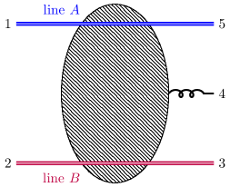
Figure 3: Graphical notation for MRK scattering. The upper double line denotes the projectile boosted in the $+$ lightcone direction, while the lower one denotes the projectile boosted along the $-$ lightcone direction. The shaded blob represents the interaction among the projectiles and the emitted gluon.

3.1 The MRK amplitude from the Balitsky/JIMWLK formalism

The Balitsky/JIMWLK formalism is a convenient framework to analyse systems with large rapidity gaps. In this formalism, in the strict high-energy limit ($x=0$), the line $A$ is represented by a single infinite Wilson line $U^{\{r\}}$, which in position space is localised on the $x_{+}=0$ lightcone and only depends non trivially on transverse coordinates $\mathbf{z}$:

$$U^{\{r\}}(z)=\mathcal{P}e^{ig_{s}\int_{-\infty}^{\infty}dx^{-}A^{a}_{-}(x^{+}=0,\,x^{-},\,\mathbf{z})T_{r}^{a}},$$ (66)

where $A$ is the gluon field, $\mathcal{P}$ is the usual path-ordering in colour space, and $r$ stands for the colour representation. Such infinite Wilson lines are divergent, and can be regulated by working at finite rapidity. Their evolution in rapidity – which generates the large $\ln x$ logs – is also known, and at LO is given by the celebrated Balitsky/JIMWLK equation. The latter is a non-linear equation and, in particular, the evolution in rapidity generates additional Wilson lines.

At finite rapidity, line $A$ can be represented as

$$a_{\lambda_{1}}^{a_{1},\dagger}(p_{1}) a_{\lambda_{5}}^{a_{5}}(p_{5})\sim 2\pi\delta(p_{1}^{+}-p_{5}^{+})\delta_{\lambda_{1}\lambda_{5}}\times 2p_{1}^{+}\times$$ (67)

$$\Big{[}\mathcal{J}({\bf q}_{A})\overline{U}_{\eta_{A}}({\bf q}_{A})+\frac{1}{2}\int\{\mathrm{d}{\bf q}\}\,\mathcal{J}^{\prime}({\bf q}_{A},{\bf q})\overline{U}_{\eta_{A}}({\bf q}_{A}-{\bf q})\overline{U}_{\eta_{A}}({\bf q})+\dots\Big{]}^{a_{1}a_{5}},$$

where $a_{\lambda_{1}}^{a_{1},\dagger}(p_{1})$ and $a_{\lambda_{5}}^{a_{5}}(p_{5})$ are creation and annihilation operators of external states. Moreover, in eq. 67, $2p_{1}^{+}$ is the standard eikonal vertex (with our definition of the lightcone coordinates), the subscript $\eta_{A}$ indicates that we have regulated the Wilson line by tilting it by a fixed rapidity $\eta_{A}=1/2\ln p_{5}^{+}/p_{5}^{-}$, and we have defined

$$\overline{U}_{\eta}({\bf p})\equiv U_{\eta}({\bf p})-\mathbb{I}\quad\text{and}\quad U_{\eta}({\bf p})=\int[\mathrm{d}{\bf z}]\,e^{-i{\bf q}\cdot{\bf z}}U_{\eta}({\bf z}).$$ (68)

We also introduced the notations

$$[\mathrm{d}{\bf z}]=\mathrm{d}^{2-2\epsilon}{\bf z},\quad\quad\{\mathrm{d}{\bf p}\}=\mathrm{d}^{2-2\epsilon}{\bf p}/(2\pi)^{2-2\epsilon}.$$ (69)

The coefficients $\mathcal{J}$ and $\mathcal{J}^{\prime}$ in eq. 67 are radiatively-generated impact factors. We note that $\mathcal{J}^{\prime}$ is a colour operator so that the product $\mathcal{J}^{\prime}\overline{U}\,\overline{U}$ is in the same representation of the $A$ projectile. In our normalisation, $\mathcal{J}\sim 1+\mathcal{O}(\alpha_{s})$ and $\mathcal{J}^{\prime}\sim\mathcal{O}(\alpha_{s})$. An analogous construction holds for line $B$, with the role of the $+$ and $-$ lightcones exchanged.

In the absence of a central gluon, to compute the amplitude one would need to evolve eq. 67 down to the rapidity $\eta_{B}=1/2\ln p_{3}^{+}/p_{3}^{-}$ – thus generating the large rapidity logs – and then compute a same-rapidity correlator with the equivalent of eq. 67 for the $B$ line, see ref. Caron-Huot:2013fea . In our case however, one first needs to evolve down to the rapidity of the central gluon ($\eta_{4}=1/2\ln p_{4}^{+}/p_{4}^{-}$), and consider the interaction of the resulting Wilson lines with the gluon 4. To the accuracy needed for this paper, it is sufficient to consider the interaction of the gluon with a single Wilson line. At LO, one can compute such interaction using the shockwave formalism, where gluon 4 interacts with the Wilson line in the background generated by projectile $B$. In terms of the annihilation operator of the emitted gluon $a_{\lambda_{4}}^{a}$, the result reads Caron-Huot:2013fea

$$\begin{split}U_{\eta}({\bf p})a^{a}_{\lambda_{4}}(p_{4})&\sim-2g_{s}\int[\mathrm{d}{\bf z}_{1}][\mathrm{d}{\bf z}_{2}]e^{-i{\bf p}\cdot{\bf z}_{1}-i{\bf p}_{4}\cdot{\bf z}_{2}}\>\big{[}U^{ab}_{\eta,\rm adj}({\bf z}_{2})\hat{T}^{b}_{1,R}-\hat{T}^{a}_{1,L}\big{]}U_{\eta}({\bf z}_{1})\times\\ &\times\int\{\mathrm{d}{\bf k}\}e^{i{\bf k}\cdot({\bf z}_{2}-{\bf z}_{1})}\>\frac{{\boldsymbol{\varepsilon}}^{*}_{\lambda_{4}}\cdot{\bf k}}{{\bf k}^{2}},\end{split}$$ (70)

where we used the standard notation

$$\begin{split}T^{a}_{i,L}\,U({\bf z}_{1})...U({\bf z}_{i})...U({\bf z}_{n})\equiv U({\bf z}_{1})...\,T^{a}U({\bf z}_{i})...U({\bf z}_{n}),\\ T^{a}_{i,R}\,U({\bf z}_{1})...U({\bf z}_{i})...U({\bf z}_{n})\equiv U({\bf z}_{1})...U({\bf z}_{i})T^{a}\,...U({\bf z}_{n}).\end{split}$$ (71)

In eq. 70, $\boldsymbol{\varepsilon}^{*}_{\lambda}$ is the two-dimensional polarisation vector of the gluon 4, with the implicit choice $\varepsilon_{\lambda}\cdot p_{2}=0$. After eq. 70 has been used, one can evolve the resulting Wilson lines down to rapidity $\eta_{B}$.

In practice, the rapidity evolution of the Wilson lines is non trivial. Fortunately, for any perturbative application, one can use the dilute-field approximation

$$U_{\eta}({\bf z})\equiv\exp\left\{ig_{s}T^{a}W_{\eta}^{a}({\bf z})\right\}=1+(ig_{s})W_{\eta}^{a}T^{a}+\frac{1}{2}(ig_{s})^{2}W_{\eta}^{a}W_{\eta}^{b}T^{a}T^{b}+\dots,$$ (72)

with $g_{s}W_{\eta}\ll 1$, see ref. Caron-Huot:2013fea for details. This allows us to perturbatively expand the shock-wave expression eq. 67 for the $A$ line, the equivalent formula for the $B$ line, and the gluon-Wilson line interaction eq. 70.

$\quad\sim\quad$ $+$ $+$ $+\quad\dots$

Figure 4: Graphical representation of the expansion of the Wilson line $A$ in terms of $W$ fields, represented by double wavy lines. The dashed blob stands for the background generated by the other projectile. A similar expansion holds for line $B$.

Introducing the Fourier conjugate of the $W$ field

$$W^{a}_{\eta}({\bf z})=\int\{\mathrm{d}{\bf q}\}e^{i{\bf q}\cdot{\bf z}}W^{a}_{\eta}({\bf q}),$$ (73)

we find that the projectile expansion eq. 67 becomes

$$a^{a_{1},\dagger}_{\lambda_{1}}(p_{1})a_{\lambda_{5}}^{a_{5}}(p_{5})\sim \,2\pi\delta(p_{1}^{+}-p_{5}^{+})\delta_{\lambda_{1}\lambda_{5}}\times 2p_{1}^{+}\times\Bigg{\{}(ig_{s})\mathcal{J}({\bf q}_{A})\llbracket W({\bf q}_{A})\rrbracket_{A}+$$

$$+\frac{(ig_{s})^{2}}{2!}\int\{\mathrm{d}{\bf q}\}\left[1+\mathcal{J}^{\prime}({\bf q}_{A},{\bf q})\right]\,\llbracket W({\bf q}_{A}-{\bf q})W({\bf q})\rrbracket_{A}+$$ (74)

$$+\frac{(ig_{s})^{3}}{3!}\int\{\mathrm{d}{\bf q}_{1}\}\{\mathrm{d}{\bf q}_{2}\}\,\llbracket W({\bf q}_{A}-{\bf q}_{1})W({\bf q}_{1}-{\bf q}_{2})W({\bf q}_{2})\rrbracket_{A}+\dots\Bigg{\}}_{\eta=\eta_{A}},$$

where we have only kept terms that contribute up to NNLL accuracy and where we have introduced the notation

$$\llbracket O_{1}O_{2}\dots O_{n}\rrbracket_{r}^{ab} \equiv(T_{r}^{c_{1}})_{aa_{1}}(T_{r}^{c_{2}})_{a_{1}a_{2}}\dots(T_{r}^{c_{n}})_{a_{n-1}b}\>O^{c_{1}}_{1}O^{c_{2}}_{2}\dots O^{c_{n}}_{n},$$ (75)

$$\llbracket O_{1}O_{2}\dots O_{n}\rrbracket^{ab} \equiv\llbracket O_{1}O_{2}\dots O_{n}\rrbracket^{ab}_{\mathrm{adj}}\,,$$

to refer to fields contracted with products of $SU(N_{c})$ generators. Graphically, section 3.1 corresponds to the expansion in fig. 4.

We now consider the interaction of a Wilson line with a gluon, and expand both sides of eq. 70 using eq. 72. After some algebra, comparing left- and right-hand sides of the equation we find that eq. 70 provides the interaction of a gluon with a single $W$ in the form

$$\begin{split}W({\bf p}&)^{b}\,a^{a}_{\lambda}(q)\sim\\ &\quad 2g_{s}\llbracket W\rrbracket^{ab}({\bf q}+{\bf p})\left[\frac{\boldsymbol{\varepsilon}^{*}_{\lambda}\cdot{\bf p}}{{\bf p}^{2}}+\frac{\boldsymbol{\varepsilon}^{*}_{\lambda}\cdot{\bf q}}{{\bf q}^{2}}\right]+\\ &+ig_{s}^{2}\int\{\mathrm{d}{\bf k}_{1}\}\llbracket W({\bf q}+{\bf p}-{\bf k}_{1})W({\bf k}_{1})\rrbracket^{ab}\left[\frac{\boldsymbol{\varepsilon}^{*}_{\lambda}\cdot{\bf p}}{{\bf p}^{2}}+\frac{\boldsymbol{\varepsilon}^{*}_{\lambda}\cdot({\bf k}_{1}-{\bf p})}{({\bf k}_{1}-{\bf p})^{2}}\right]+\\ &+g_{s}^{3}\int\{\mathrm{d}{\bf k}_{1}\}\{\mathrm{d}{\bf k}_{2}\}\llbracket W({\bf q}+{\bf p}-{\bf k}_{1})W({\bf k}_{1}-{\bf k}_{2})W({\bf k}_{2})\rrbracket^{ab}\times\\ &\times\bigg{[}\frac{1}{6}\left(\frac{\boldsymbol{\varepsilon}^{*}_{\lambda}\cdot({\bf k}_{1}-{\bf p})}{({\bf k}_{1}-{\bf p})^{2}}\right)-\frac{1}{2}\left(\frac{\boldsymbol{\varepsilon}^{*}_{\lambda}\cdot({\bf k}_{2}-{\bf p})}{({\bf k}_{2}-{\bf p})^{2}}\right)-\frac{1}{3}\left(\frac{\boldsymbol{\varepsilon}^{*}_{\lambda}\cdot{\bf p}}{{\bf p}^{2}}\right)\bigg{]}+\dots,\end{split}$$ (76)

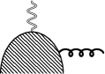
$\quad\sim\quad$ $+$ $+$ $+\quad\dots$

Figure 5: Graphical representation of eq. 76. The shaded area represents the background generated by line $B$, while the black dots correspond to interactions “vertices”. Similar diagrams can be drawn for eqs. 77 and 78 by simply replacing the upper $W$ field with two and three $W$ fields respectively.

for which we provide a cartoon in fig. 5. We also find the interactions with multiple $W$ fields to be

$$[W^{b}\otimes W^{c}]({\bf p})\,a_{\lambda}^{a}(q) \sim 2g_{s}\int\{\mathrm{d}{\bf k}_{1}\}\llbracket W({\bf q}+{\bf p}-{\bf k}_{1})\rrbracket^{ab}W^{c}({\bf k}_{1})\times$$

$$\times\left[\frac{\boldsymbol{\varepsilon}^{*}_{\lambda}\cdot{\bf q}}{{\bf q}^{2}}+\frac{\boldsymbol{\varepsilon}^{*}_{\lambda}\cdot({\bf p}-{\bf k}_{1})}{({\bf p}-{\bf k}_{1})^{2}}\right]+(b\leftrightarrow c)+\dots,$$ (77)

$$[W^{b}\otimes W^{c}\otimes W^{d}]({\bf p})\,a^{a}_{\lambda}(q) \sim 2g_{s}\int\{\mathrm{d}{\bf k}_{1}\}\{\mathrm{d}{\bf k}_{2}\}\llbracket W({\bf q}+{\bf p}-{\bf k}_{1})\rrbracket^{ab}W^{c}({\bf k}_{1}-{\bf k}_{2})W^{d}({\bf k}_{2})\times$$

$$\times\left[\frac{\boldsymbol{\varepsilon}^{*}_{\lambda}\cdot{\bf q}}{{\bf q}^{2}}+\frac{\boldsymbol{\varepsilon}^{*}_{\lambda}\cdot({\bf p}-{\bf k}_{1})}{({\bf p}-{\bf k}_{1})^{2}}\right]+(b\leftrightarrow c)+(b\leftrightarrow d)+\dots,$$ (78)

where $[f\otimes g]({\bf q})=\int\{\mathrm{d}{\bf k}\}f({\bf k})g({\bf q}-{\bf k})$ is the standard Fourier convolution and where we refrain from writing expressions for interactions with more than 3 $W$s as well as higher order terms since they will not play any role in our analysis. As we have mentioned, eqs. 76, 77 and 78 receive perturbative corrections. However, in the next subsection we will see that for the purposes of this paper the only relevant ones are those affecting the first term on the right-hand side of eq. 76, which gets dressed with a radiative vertex correction $\mathcal{W}_{\lambda}=1+\mathcal{O}(\alpha_{s})$ yielding

$$\begin{split}2g_{s}\llbracket W\rrbracket^{ab}({\bf q}+{\bf p})&\left[\frac{\boldsymbol{\varepsilon}^{*}_{\lambda}\cdot{\bf p}}{{\bf p}^{2}}+\frac{\boldsymbol{\varepsilon}^{*}_{\lambda}\cdot{\bf q}}{{\bf q}^{2}}\right]\longrightarrow\\ &2g_{s}\llbracket W\rrbracket^{ab}({\bf q}+{\bf p})\left[\frac{\boldsymbol{\varepsilon}^{*}_{\lambda}\cdot{\bf p}}{{\bf p}^{2}}+\frac{\boldsymbol{\varepsilon}^{*}_{\lambda}\cdot{\bf q}}{{\bf q}^{2}}\right]\mathcal{W}_{\lambda}({\bf p},{\bf q}).\end{split}$$ (79)

We conclude by reporting some of the main features of the $W$ field, once again referring the reader to ref. Caron-Huot:2013fea for additional details. Up to two loops, $W$ is an eigenstate of the Balitsky/JIMWLK rapidity evolution, and its eigenvalue coincides with (minus) the gluon Regge trajectory $\tau_{g}$:

$$-\frac{\mathrm{d}}{\mathrm{d}\eta}W_{\eta}({{\bf p}})=\tau_{g}({\bf p})W_{\eta}({\bf p}).$$ (80)

Explicit results for $\tau_{g}$ up to two loops are reported in section 4.3. We note that the rapidity evolution also induces transitions between $n$ and $n+2$, $n+4$ etc. states, but such transitions are suppressed by at least one power of $\alpha_{s}$ compared to the $n\to n$ ones, and do not enter in our analysis.

At LO the $W$ fields are free, so that their same-rapidity correlator is

$$\Big{\langle}\mathbb{T}\big{[}W({\bf p}_{1})\cdots W({\bf p}_{n})\big{]}_{\eta}\big{[}\widetilde{W}({\bf q}_{1})\cdots\widetilde{W}({\bf q}_{m})\big{]}_{\eta}\Big{\rangle}=$$ (81)

$$\delta_{nm}\sum_{\sigma\in S_{n}}G({\bf p}_{1},{\bf q}_{\sigma(1)})\dots G({\bf p}_{n},{\bf q}_{\sigma(n)})+\mathcal{O}(\alpha_{s}),$$

where $\mathbb{T}$ is the standard time ordering, $\widetilde{W}$ is associated with projectile $B$, and the 2-point correlator reads

$$G({\bf p},{\bf q})=\Big{\langle}\mathbb{T}\,W^{a}_{\eta}({\bf p})\widetilde{W}^{b}_{\eta}({\bf q})\Big{\rangle}=(2\pi)^{2-2\epsilon}\delta^{2-2\epsilon}({\bf p}-{\bf q})\frac{i\delta^{ab}}{{\bf p}^{2}}+\mathcal{O}(\alpha_{s}).$$ (82)

Due to CPT invariance, the correlator between even and odd numbers of $W$ fields is zero at any order ($W$ is a signature-odd field) Caron-Huot:2013fea . Beyond LO, it is convenient to redefine the $W$ field

$$W\to(1+\alpha_{s}r_{1}+\dots)W+(\alpha_{s}^{2}s_{1}+\dots)WWW+\dots,$$ (83)

such that $a)$ correlators with different numbers of $W$ fields on the two lightcones vanish,

$$\Big{\langle}\mathbb{T}\big{[}W({\bf p}_{1})\cdots W({\bf p}_{n})\big{]}_{\eta}\big{[}\widetilde{W}({\bf q}_{1})\cdots\widetilde{W}({\bf q}_{m})\big{]}_{\eta}\Big{\rangle}=0\quad\quad\text{for}\quad n\neq m,$$ (84)

and $b)$ the two-point correlator is equal to the free one

$$G({\bf p},{\bf q})=\Big{\langle}\mathbb{T}\,W^{a}_{\eta}({\bf p})\widetilde{W}^{b}_{\eta}({\bf q})\Big{\rangle}=(2\pi)^{2-2\epsilon}\delta^{2-2\epsilon}({\bf p}-{\bf q})\frac{i\delta^{ab}}{{\bf p}^{2}},$$ (85)

at any order in $\alpha_{s}$. Note that after this redefinition eq. 72 would not hold anymore, but sections 3.1 and 80 still hold (with modified impact factors, but unchanged gluon Regge trajectory) and our computation remains identical to the required order.

These are all the details that we need to predict the MRK behaviour of the 5-point scattering amplitude up to two loops. We study this in the next subsections. We start by discussing the $(--)$ signature, which is the only one that contributes at LL and NLL accuracy at the cross-section level, see e.g. ref. BARTELS1980365 .

3.2 LL and NLL predictions for the MRK amplitudes

3.2.1 LL and NLL predictions for the $(--)$ signature

To obtain a prediction for the LL amplitude in the formalism summarised in the previous section, we recall that large logarithms are only generated by the rapidity evolution. Because of this, and because multiple $W$ contributions are suppressed by powers of $g_{s}$, cf. section 3.1, only the single-$W$ term in section 3.1 contributes at LL. For the same reason, no perturbative corrections to the impact factors enter in the LL approximation, i.e. $\mathcal{J}_{X}\to 1$. Up to an overall – hence immaterial – phase $\phi^{[AB]}$ that depends on spinor conventions, the connected $S$-matrix element eq. 16 that we need to consider is then

$$\mathcal{S}_{\mathrm{LL}} =\phi^{[AB]}\left[2\pi\delta(p_{1}^{+}-p_{5}^{+})\delta_{\lambda_{1}\lambda_{5}}\times 2p_{1}^{+}\right]\left[2\pi\delta(p_{2}^{-}-p_{3}^{-})\delta_{\lambda_{2}\lambda_{3}}\times 2p_{2}^{-}\right]$$ (86)

$$\times\bigg{\langle}\mathbb{T}\,\Big{(}ig_{s}\llbracket W_{\eta_{A}}({\bf q}_{A})\rrbracket^{c_{5}c_{1}}_{r_{A}}\Big{)}a^{a_{4}}_{\lambda_{4}}(p_{4})\Big{(}ig_{s}\llbracket\widetilde{W}_{\eta_{B}}({\bf q}_{B})\rrbracket^{c_{3}c_{2}}_{r_{B}}\Big{)}\bigg{\rangle}\,.$$

To evaluate this correlator, we first use eq. 80 to evolve the $W_{\eta_{A}}({\bf q}_{A})$ field to central rapidity

$$W^{a}_{\eta_{A}}({\bf q}_{A})=e^{\Delta\eta_{A4}\tau_{g}({\bf q}_{A})}W^{a}_{\eta_{4}}({\bf q}_{A}),$$ (87)

where at LL we only require the LO (i.e. $\mathcal{O}(\alpha_{s})$) Regge trajectory. It reads

$$\left(\frac{\alpha_{s}}{4\pi}\right)\tau^{(1)}_{g}({\bf q})=\left(\frac{\alpha_{s}}{4\pi}\right)2N_{c}\frac{e^{\epsilon\gamma_{E}}\Gamma(1-\epsilon)^{2}\Gamma(1+\epsilon)}{\Gamma(1-2\epsilon)\epsilon}\left(\frac{\mu^{2}}{{\bf q}^{2}}\right)^{\epsilon},$$ (88)

with $\gamma_{E}$ the Eulero-Mascheroni constant, $\gamma_{E}\approx 0.577216$. At small $x$, the rapidity difference can be written as

$$\Delta\eta_{ij}=\eta_{i}-\eta_{j}=\ln\frac{|s_{ij}|}{|{\bf p}_{i}||{\bf p}_{j}|}+\mathcal{O}(x).$$ (89)

We remind the reader that $\eta_{A}=1/2\ln p_{5}^{+}/p_{5}^{-}$ and $\eta_{B}=1/2\ln p_{3}^{+}/p_{3}^{-}$. As a next step, we apply eq. 76 to compute the LO interaction of $W^{a}_{\eta_{4}}({\bf q}_{A})$ with the emitted gluon

$$W^{a}_{\eta_{4}}({\bf q}_{A})a_{\lambda_{4}}^{a_{4}}(p_{4})\to 2g_{s}\llbracket W\rrbracket^{a_{4}a}_{\eta_{4}}({\bf q}_{A}+{\bf p}_{4})\left[\frac{\boldsymbol{\varepsilon}^{*}_{\lambda_{4}}\cdot{\bf p}_{4}}{{\bf p}_{4}^{2}}+\frac{\boldsymbol{\varepsilon}^{*}_{\lambda_{4}}\cdot{\bf q}_{A}}{{\bf q}_{A}^{2}}\right]+\dots,$$ (90)

and finally evolve the resulting $W$ field from rapidity $\eta_{4}$ to rapidity $\eta_{B}$, and compute the equal-rapidity correlator eq. 85. Using eq. 16, we can then write a LL prediction for the amplitude:

$$\mathcal{A}_{\text{LL}}=\mathcal{A}^{(--)}_{\text{LL}}=\phi^{[AB]} \,4g_{s}^{3}s_{12}\left[(T_{r_{B}})_{c_{3}c_{2}}^{b}(T_{r_{A}})_{c_{5}c_{1}}^{a}if^{aba_{4}}\right]\times$$ (91)

$$e^{\tau_{g}({\bf q}_{A})\Delta\eta_{A4}}\frac{1}{{\bf q}_{B}^{2}}\left[\frac{\boldsymbol{\varepsilon}^{*}_{\lambda_{4}}\cdot{\bf p}_{4}}{{\bf p}_{4}^{2}}+\frac{\boldsymbol{\varepsilon}^{*}_{\lambda_{4}}\cdot{\bf q}_{A}}{{\bf q}_{A}^{2}}\right]e^{\tau_{g}({\bf q}_{B})\Delta\eta_{4B}}.$$

Using the explicit results for the polarisation vectors in appendix A, the term in the square bracket can be written as

$$\left[\frac{\boldsymbol{\varepsilon}^{*}_{\lambda_{4}}\cdot{\bf p}_{4}}{{\bf p}_{4}^{2}}+\frac{\boldsymbol{\varepsilon}^{*}_{\lambda_{4}}\cdot{\bf q}_{A}}{{\bf q}_{A}^{2}}\right]=\frac{1}{\sqrt{2}}\times V_{\lambda_{4}}({\bf q}_{A},{\bf p}_{4})\times\frac{1}{{\bf q}_{A}^{2}},$$ (92)

with

$$V_{+}({\bf q}_{A},{\bf p}_{4})=\frac{\bar{q}_{A,\perp}\,q_{B,\perp}}{p_{4,\perp}},\quad\quad V_{-}({\bf q}_{A},{\bf p}_{4})=\frac{q_{A,\perp}\,\bar{q}_{B,\perp}}{\bar{p}_{4,\perp}},$$ (93)

where we used the complex notation $p_{\perp}=p^{x}+ip^{y}$, $\bar{p}_{\perp}=p^{x}-ip^{y}$, see appendix A. The function $V_{\lambda}$ in eq. 93 is the LO Lipatov vertex, or central emission vertex, which is a critical ingredient for computing amplitudes in the MRK, see e.g. ref. DelDuca:2022skz and references therein.

In terms of the Lipatov vertex, the LL amplitude can be written in the suggestive form

$$\begin{split}&\mathcal{A}^{(--)}_{\text{LL}}=\phi^{[AB]}\,2\sqrt{2}\,g_{s}^{3}s_{12}\\ &\quad\times(T_{r_{A}})_{c_{5}c_{1}}^{a}e^{\tau_{g}({\bf q}_{A})\Delta\eta_{A4}}\frac{1}{{\bf q}_{A}^{2}}\left[if^{aba_{4}}V_{\lambda_{4}}({\bf q}_{A},{\bf p}_{4})\right]\frac{1}{{\bf q}_{B}^{2}}e^{\tau_{g}({\bf q}_{B})\Delta\eta_{4B}}(T_{r_{B}})_{c_{3}c_{2}}^{b},\end{split}$$ (94)

where the $t$-channel exchange structure is apparent. Repeating the same steps we performed here for the $2\to n$ amplitude in MRK, it is straightforward to see that such a structure iterates at all multiplicities. We briefly discuss this in section 3.3, but first we give explicit expressions for the phase factors $\phi^{[AB]}$. These depend on the spinor conventions adopted. To fix them, we match eq. 94 against eq. 17, remembering that in MRK only the signature-odd amplitude with colour-octet exchange in both the 1–5 and 2–3 channels is non vanishing at LO, see eq. 46. Using the spinor conventions of appendix A, for the helicity choices in eq. 19 we obtain

$$\phi^{[gg]}=\frac{\bar{p}_{3,\perp}}{p_{3,\perp}},\quad\phi^{[qg]}=-i\frac{\bar{p}_{3,\perp}}{p_{3,\perp}},\quad\phi^{[qQ]}=\frac{\bar{p}_{3,\perp}}{|p_{3,\perp}|}.$$ (95)

The same procedure can be applied to all other helicites. Since the $\phi^{[AB]}$ phase is immaterial, we refrain from reporting here explicit formulas for all the other possible helicity configurations.

We now discuss the NLL generalisation of eq. 94. As we have mentioned in section 3.1, $W$ is a signature-odd field. As a consequence, the $(--)$ amplitudes only receives contributions when an odd number of $W$ is emitted from both the $A$ and $B$ lines. Simple power counting then shows that only one-$W$ exchanges arise at NLL, making the NLL generalisation of the LL results above straightforward. Indeed, the factorised form of the amplitude eq. 94 remains basically unchanged, except for the addition of (multiplicative) radiative corrections for the impact factors $\mathcal{J}$ section 3.1 and the $WWg$ interaction vertex $\mathcal{W}_{\lambda}$ eq. 79. The NLL amplitude then reads

$$\begin{split}&\mathcal{A}^{(--)}_{\text{NLL}}=\phi^{[AB]}\,2\sqrt{2}\,g_{s}^{3}s_{12}\times(T_{r_{A}})_{c_{5}c_{1}}^{a}\mathcal{J}({\bf q}_{A})e^{\tau_{g}({\bf q}_{A})\Delta\eta_{A4}}\\ &\quad\times\frac{1}{{\bf q}_{A}^{2}}\left[if^{aba_{4}}V_{\lambda_{4}}({\bf q}_{A},{\bf p}_{4})\mathcal{W}_{\lambda_{4}}({\bf q}_{A},{\bf p}_{4})\right]\frac{1}{{\bf q}_{B}^{2}}e^{\tau_{g}({\bf q}_{B})\Delta\eta_{4B}}\mathcal{J}({\bf q}_{B})(T_{r_{B}})_{c_{3}c_{2}}^{b}.\end{split}$$ (96)

At this order, one only needs $\mathcal{O}(\alpha_{s})$ corrections to the impact factors $\mathcal{J}$ and vertex $\mathcal{W}$, but two-loop $\mathcal{O}(\alpha_{s}^{2})$ corrections to the gluon Regge trajectory $\tau_{g}$. Both $\mathcal{J}$ and the Regge trajectory can be extracted from the $2\to 2$ scattering amplitude, thus allowing one to obtain the one-loop contribution to $\mathcal{W}_{\lambda}$ by matching eq. 96 to the one-loop $2\to 3$ amplitude. To compare NLL results with the literature, we find it convenient to perform a redefinition of the evolution variable, impact factors $\mathcal{J}$, and vertex $\mathcal{W}$. However, before elaborating on this, we discuss NLL predictions for the other signatures at one loop.

3.2.2 One-loop NLL predictions for the other signatures

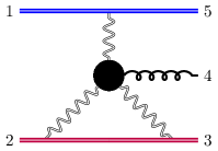
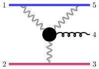
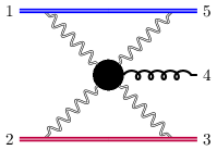
Figure 6: Schematic diagrams for multi-$W$ contributions to the the $(-+)$, $(+-)$, and $(++)$ one-loop amplitudes.

We consider one-loop amplitudes with signatures $(-+)$, $(+-)$ and $(++)$ up to NLL, starting from the former. The $(-+)$ amplitude only receives contributions where an odd number of $W$ fields are emitted from the $A$ line, and an even one from the $B$ line. Since each $W$ is accompanied by a $g_{s}$ factor without any large logarithm, see section 3.1, at NLL we need to consider the emission of one $W$ from the $A$ and two $W$s from the $B$ line. The rapidity evolution is signature preserving (see the discussion around eq. 80), hence the only non-vanishing contribution at NLL comes from the $W\to WW$ transition, cf. the second line of eq. 76 and fig. 6. Crucially, this is $\mathcal{O}(g_{s})$ with respect to the LL result. As a consequence, to NLL accuracy the $W$ fields can be treated at LO. This makes NLL predictions for the $(-+)$ signature conceptually trivial. The only subtlety is that the two-$W$ state is not an eigenstate of the rapidity evolution Hamiltonian, hence a simple exponentiation like in eq. 87 does not hold. However, the effect of the evolution starts appearing at the two-loop ($\alpha_{s}^{2}L$) order. Here we focus on the one-loop amplitude, the evolution then does not play any role and we can immediately write down the NLL result.

By combining the appropriate terms in sections 3.1 and 76, we find

$$\mathcal{S} {}^{(-+)}_{\mathrm{NLL}}=$$ (97)

$$=\phi^{[AB]}\left[2\pi\delta(p_{1}^{+}-p_{5}^{+})\delta_{\lambda_{1}\lambda_{5}}\times 2p_{1}^{+}\right]\left[2\pi\delta(p_{2}^{-}-p_{3}^{-})\delta_{\lambda_{2}\lambda_{3}}\times 2p_{2}^{-}\right]$$

$$\times\Bigg{\langle}\mathbb{T}\,\Big{(}ig_{s}\llbracket W_{\eta_{A}}({\bf q}_{A})\rrbracket^{c_{5}c_{1}}_{r_{A}}\Big{)}a^{a_{4}}_{\lambda_{4}}(p_{4})\Bigg{(}\frac{(ig_{s})^{2}}{2!}\llbracket\widetilde{W}_{\eta_{B}}\otimes\widetilde{W}_{\eta_{B}}\rrbracket^{c_{3}c_{2}}_{r_{B}}({\bf q}_{B})\Bigg{)}\Bigg{\rangle}\,=$$

$$=\phi^{[AB]}\left[2\pi\delta(p_{1}^{+}-p_{5}^{+})\delta_{\lambda_{1}\lambda_{5}}\right]\left[2\pi\delta(p_{2}^{-}-p_{3}^{-})\delta_{\lambda_{2}\lambda_{3}}\right]\times 4s_{12}$$

$$\times\left[ig_{s}(T_{r_{A}}^{a})_{c_{5}c_{1}}\right]\times ig_{s}^{2}\int\{\mathrm{d}{\bf k}_{1}\}\left[\frac{\boldsymbol{\varepsilon}^{*}_{\lambda}\cdot{\bf q}_{A}}{{\bf q}_{A}^{2}}+\frac{\boldsymbol{\varepsilon}^{*}_{\lambda}\cdot({\bf k}_{1}-{\bf q}_{A})}{({\bf k}_{1}-{\bf q}_{A})^{2}}\right]$$

$$\times\Bigg{\langle}\mathbb{T}\,\llbracket W_{\eta_{4}}({\bf q}_{A}+{\bf p}_{4}-{\bf k}_{1})W_{\eta_{4}}({\bf k}_{1})\rrbracket^{a_{4}a}\Bigg{(}\frac{(ig_{s})^{2}}{2!}\llbracket\widetilde{W}_{\eta_{B}}\otimes\widetilde{W}_{\eta_{B}}\rrbracket^{c_{3}c_{2}}_{r_{B}}({\bf q}_{B})\Bigg{)}\Bigg{\rangle}.$$

The equivalent result for the amplitude, see eq. 16, reads

$$\begin{split}\mathcal{A}_{\text{NLL}}^{(-+)}&=4ig_{s}^{3}\phi^{[AB]}s_{12}\left[(T_{r_{A}})_{c_{5}c_{1}}^{a}if^{a_{4}a_{1}e}if^{ea_{2}a}(\delta_{a_{1}b_{1}}\delta_{a_{2}b_{2}}+\delta_{a_{1}b_{2}}\delta_{a_{2}b_{1}})(T_{r_{B}}^{b_{1}}\!\cdot\!T_{r_{B}}^{b_{2}})_{c_{3}c_{2}}\right]\\ &\times\frac{g_{s}^{2}}{4}\int\{\mathrm{d}{\bf k}_{1}\}\frac{1}{({\bf q}_{B}-{\bf k}_{1})^{2}}\frac{1}{{\bf k}_{1}^{2}}\left[\frac{\boldsymbol{\varepsilon}^{*}_{\lambda}\cdot{\bf q}_{A}}{{\bf q}_{A}^{2}}+\frac{\boldsymbol{\varepsilon}^{*}_{\lambda}\cdot({\bf k}_{1}-{\bf q}_{A})}{({\bf k}_{1}-{\bf q}_{A})^{2}}\right]\big{(}1+\mathcal{O}(\alpha_{s})\big{)}.\end{split}$$ (98)

We now look at the colour structure of eq. 98. To do so, we introduce the graphic notation

$$\includegraphics[valign={m}]{tikz-fig/fig_3.pdf},\quad\quad\includegraphics[valign={m}]{tikz-fig/fig_4.pdf}\,,$$ (99)

in terms of which we can write the Lie algebra identity

$$[T^{a}_{r_{A}},T^{b}_{r_{A}}]=if^{abc}T_{r_{A}}^{c}\rightarrow\includegraphics[valign={m}]{tikz-fig/fig_5.pdf}=\includegraphics[valign={m}]{tikz-fig/fig_6.pdf}-\includegraphics[valign={m}]{tikz-fig/fig_7.pdf}.$$ (100)

In this notation, the colour structure of eq. 98 can be written as

$$T_{r_{A}}^{a}if^{aa_{2}e}if^{ea_{1}a_{4}}(\delta_{a_{1}b_{1}}\delta_{a_{2}b_{2}}+\delta_{a_{1}b_{2}}\delta_{a_{2}b_{1}})(T_{r_{B}}^{b_{1}}\!\cdot\!T_{r_{B}}^{b_{2}})\rightarrow\includegraphics[valign={m}]{tikz-fig/fig_8.pdf}+\includegraphics[valign={m}]{tikz-fig/fig_9.pdf}.$$ (101)

After simple manipulations, using eq. 100 we obtain

$$\includegraphics[valign={m}]{tikz-fig/fig_10.pdf}+\includegraphics[valign={m}]{tikz-fig/fig_11.pdf} =-\includegraphics[valign={m}]{tikz-fig/fig_12.pdf}+\includegraphics[valign={m}]{tikz-fig/fig_13.pdf}+\includegraphics[valign={m}]{tikz-fig/fig_14.pdf}-\includegraphics[valign={m}]{tikz-fig/fig_15.pdf}$$ (102)

$$=-\boldsymbol{\mathcal{T}}_{+-}\,\includegraphics[valign={m}]{tikz-fig/fig_16.pdf},$$

where we have coloured in purple the underlying tree-level colour structure and identified the remaining black gluons in terms of the colour operators ${\bf T}^{\pm}_{ij}$ in eq. 23. We then combined these into $\boldsymbol{\mathcal{T}}_{+-}$, defined in eq. 30.

Using eq. 102, we can write the amplitude eq. 98 as

$$\begin{split}\mathcal{A}_{\text{NLL}}^{(-+)}&=-i\pi\left[\frac{g_{s}^{2}S_{\epsilon}}{(4\pi)^{2}}\right]\mathcal{K}^{(1)}_{\{1,2\}}\boldsymbol{\mathcal{T}}_{+-}\mathcal{A}^{(0)}\left(1+\mathcal{O}(\alpha_{s})\right)=\\ &=-i\pi\left(\frac{\alpha_{s}}{4\pi}\right)\mathcal{K}^{(1)}_{\{1,2\}}\boldsymbol{\mathcal{T}}_{+-}\mathcal{A}^{(0)}\left(1+\mathcal{O}(\alpha_{s})\right),\end{split}$$ (103)

or

$$\mathcal{A}_{\text{NLL}}^{(1),(-+)}=-i\pi\mathcal{K}^{(1)}_{\{1,2\}}\boldsymbol{\mathcal{T}}_{+-}\mathcal{A}^{(0)}.$$ (104)

In these equations, $S_{\epsilon}=(4\pi)^{\epsilon}e^{-\epsilon\gamma_{E}}$ is the standard $\overline{\rm MS}$ renormalisation factor,

$$\mathcal{K}^{(1)}_{\{1,2\}}=\left[\mathcal{K}^{(0)}_{\{1,1\}}\right]^{-1}\int\frac{\mathfrak{D}{\bf k}_{1}}{{\bf k}_{1}^{2}({\bf q}_{B}-{\bf k}_{1})^{2}}\left[\frac{\boldsymbol{\varepsilon}^{*}_{\lambda}\cdot{\bf q}_{A}}{{\bf q}_{A}^{2}}+\frac{\boldsymbol{\varepsilon}^{*}_{\lambda}\cdot({\bf k}_{1}-{\bf q}_{A})}{({\bf k}_{1}-{\bf q}_{A})^{2}}\right],$$ (105)

with $\mathfrak{D}p=(\mu^{2\epsilon}e^{\epsilon\gamma_{E}}/\pi^{1-\epsilon})\mathrm{d}^{2-2\epsilon}p$, and

$$\mathcal{K}^{(0)}_{\{1,1\}}=\frac{1}{{\bf q}_{B}^{2}}\left[\frac{\boldsymbol{\varepsilon}^{*}_{\lambda_{4}}\cdot{\bf p}_{4}}{{\bf p}_{4}^{2}}+\frac{\boldsymbol{\varepsilon}^{*}_{\lambda_{4}}\cdot{\bf q}_{A}}{{\bf q}_{A}^{2}}\right].$$ (106)

We note that all the functions $\mathcal{K}^{(l)}_{\{i,j\}}$ depend on the gluon polarisation $\lambda_{4}$. We have left this dependence implicit. We discuss these functions in more detail in appendix D; here we limit ourselves to say that they are pure (i.e. they have no rational prefactors), of uniform transcendental weight, and that the $\lambda_{4}$ dependence starts at $\mathcal{O}(\epsilon)$. Up to finite terms, for both positive and negative gluon helicities we obtain

$$\mathcal{K}^{(1)}_{\{1,2\}}=-\frac{1}{\epsilon}+\ln\left(\frac{{\bf q}_{B}^{2}{\bf p}_{4}^{2}}{{\bf q}_{A}^{2}\mu^{2}}\right)+\mathcal{O}(\epsilon).$$ (107)

Generic expressions at higher orders in $\epsilon$ can be found in appendix D.

We can repeat the same procedure to obtain the $(+-)$ one-loop amplitude, with the important difference that the rapidity evolution and $W$/gluon expansion have to be performed from $B$ to $A$, fig. 6. We remind the reader that the formulas for $W$/gluon interactions in section 3.1 have been obtained by making a reference choice for the emitted gluon such that its polarisation vector does not have components on the large lightcone direction, $\varepsilon_{4}\cdot p_{2}=0$ for the evolution from $A$ to $B$. If we evolve instead from $B$ to $A$, we can use the same formulas but have now to impose $\varepsilon_{4}\cdot p_{1}=0$. To differentiate polarisation vectors with different reference choices, we refer to the transverse components in the $\varepsilon\cdot p_{2}=0$ case by ${\boldsymbol{\varepsilon}}$ and to those in the $\varepsilon\cdot p_{1}=0$ by $\boldsymbol{\widetilde{\varepsilon}}$, see appendix A for more details and explicit representations.

Apart from this caveat the calculation proceeds exactly like in the $(-+)$ case, and we obtain

$$\mathcal{A}^{(1),(+-)}_{\text{NLL}}=-i\pi\mathcal{K}^{(1)}_{\{2,1\}}\boldsymbol{\mathcal{T}}_{-+}\mathcal{A}^{(0)},$$ (108)

with now

$$\mathcal{K}^{(1)}_{\{2,1\}}=\left[\widetilde{\mathcal{K}}^{(0)}_{\{1,1\}}\right]^{-1}\int\frac{\mathfrak{D}{\bf k}_{1}}{{\bf k}_{1}^{2}({\bf q}_{A}+{\bf k}_{1})^{2}}\left[-\frac{\boldsymbol{\widetilde{\varepsilon}}^{*}_{\lambda}\cdot{\bf q}_{B}}{{\bf q}_{B}^{2}}+\frac{\boldsymbol{\widetilde{\varepsilon}}^{*}_{\lambda}\cdot({\bf k}_{1}+{\bf q}_{B})}{({\bf k}_{1}+{\bf q}_{B})^{2}}\right],$$ (109)

and

$$\widetilde{\mathcal{K}}^{(0)}_{\{1,1\}}=\frac{1}{{\bf q}_{A}^{2}}\left[\frac{\boldsymbol{\widetilde{\varepsilon}}^{*}_{\lambda_{4}}\cdot{\bf p}_{4}}{{\bf p}_{4}^{2}}-\frac{\boldsymbol{\widetilde{\varepsilon}}^{*}_{\lambda_{4}}\cdot{\bf q}_{B}}{{\bf q}_{B}^{2}}\right].$$ (110)

Up to finite terms, eq. 109 reads

$$\mathcal{K}^{(1)}_{\{2,1\}}=-\frac{1}{\epsilon}+\ln\left(\frac{{\bf q}_{A}^{2}{\bf p}_{4}^{2}}{{\bf q}_{B}^{2}\mu^{2}}\right)+\mathcal{O}(\epsilon).$$ (111)

We note that the result eq. 108 can also be immediately obtained from eq. 104 by simply exchanging the two lightcones. As discussed at the end of section 2.1, this amounts to the kinematics exchange $z\leftrightarrow 1-\bar{z}$ (which in eqs. 107 and 111 simply amounts to the the ${\bf p}_{3}\leftrightarrow{\bf p}_{5}$ exchange), followed by an appropriate permutation in the colour operators.

The last signature we need to consider is $(++)$, see fig. 6. We write the connected $S$-matrix for the emission of two $W$ from each of the $A$ and $B$ lines as

$$\mathcal{S} {}^{(++)}_{\mathrm{NLL}}=$$ (112)

$$=\phi^{[AB]}\left[2\pi\delta(p_{1}^{+}-p_{5}^{+})\delta_{\lambda_{1}\lambda_{5}}\times 2p_{1}^{+}\right]\left[2\pi\delta(p_{2}^{-}-p_{3}^{-})\delta_{\lambda_{2}\lambda_{3}}\times 2p_{2}^{-}\right]$$

$$\times\Bigg{\langle}\mathbb{T}\,\Bigg{(}\frac{(ig_{s})^{2}}{2!}\llbracket W_{\eta_{A}}\!\otimes\!W_{\eta_{A}}\rrbracket^{c_{5}c_{1}}_{r_{A}}({\bf q}_{A})\Bigg{)}a^{a_{4}}_{\lambda_{4}}(p_{4})\Bigg{(}\frac{(ig_{s})^{2}}{2!}\llbracket\widetilde{W}_{\eta_{B}}\!\otimes\!\widetilde{W}_{\eta_{B}}\rrbracket^{c_{3}c_{2}}_{r_{B}}({\bf q}_{B})\Bigg{)}\Bigg{\rangle}\,=$$

$$=\phi^{[AB]}\left[2\pi\delta(p_{1}^{+}-p_{5}^{+})\delta_{\lambda_{1}\lambda_{5}}\right]\left[2\pi\delta(p_{2}^{-}-p_{3}^{-})\delta_{\lambda_{2}\lambda_{3}}\right]\times 4s_{12}$$

$$\times\left[\frac{(ig_{s})^{2}}{2!}\left(T_{r_{A}}^{(d_{1}}\!\cdot\!T_{r_{A}}^{d_{2})}\right)_{c_{5}c_{1}}\right]\times 2g_{s}\int\{\mathrm{d}{\bf k}_{1}\}\left[\frac{\boldsymbol{\varepsilon}^{*}_{\lambda}\cdot{\bf p}_{4}}{{\bf p}_{4}^{2}}+\frac{\boldsymbol{\varepsilon}^{*}_{\lambda}\cdot({\bf q}_{A}-{\bf k}_{1})}{({\bf q}_{A}-{\bf k}_{1})^{2}}\right]$$

$$\times\Bigg{\langle}\mathbb{T}\,\llbracket W_{\eta_{4}}({\bf q}_{A}+{\bf p}_{4}-{\bf k}_{1})\rrbracket^{a_{4}d_{1}}W_{\eta_{4}}^{d_{2}}({\bf k}_{1})\Bigg{(}\frac{(ig_{s})^{2}}{2!}\llbracket\widetilde{W}_{\eta_{B}}\otimes\widetilde{W}_{\eta_{B}}\rrbracket^{c_{3}c_{2}}_{r_{B}}({\bf q}_{B})\Bigg{)}\Bigg{\rangle},$$

where we used the notation $T_{r}^{(i_{1}}\!\cdot\!T_{r}^{i_{2})}=T_{r}^{i_{1}}\!\cdot\!T_{r}^{i_{2}}+T_{r}^{i_{2}}\!\cdot\!T_{r}^{i_{1}}$. This leads to the one-loop amplitude

$$\begin{split}\mathcal{A}^{(++)}_{\text{NLL}}&=4ig_{s}^{3}\phi^{[AB]}s_{12}\left[\left(T_{r_{A}}^{(d_{1}}\!\cdot\!T_{r_{A}}^{d_{2})}\right)_{c_{5}c_{1}}if^{a_{4}b_{1}d_{1}}\left(T_{r_{B}}^{(b_{1}}\!\cdot\!T_{r_{B}}^{d_{2})}\right)_{c_{3}c_{2}}\right]\\ &\times\frac{g_{s}^{2}}{4}\int\{\mathrm{d}{\bf k}_{1}\}\frac{1}{({\bf q}_{B}-{\bf k}_{1})^{2}}\frac{1}{{\bf k}_{1}^{2}}\left[\frac{\boldsymbol{\varepsilon}^{*}_{\lambda}\cdot{\bf p}_{4}}{{\bf p}_{4}^{2}}+\frac{\boldsymbol{\varepsilon}^{*}_{\lambda}\cdot({\bf q}_{A}-{\bf k}_{1})}{({\bf q}_{A}-{\bf k}_{1})^{2}}\right]\big{(}1+\mathcal{O}(\alpha_{s})\big{)}.\end{split}$$ (113)

The colour algebra now reads

$$\left(T_{r_{A}}^{(d_{1}}\!\cdot\!T_{r_{A}}^{d_{2})}\right)_{c_{5}c_{1}}if^{a_{4}b_{1}d_{1}}\left(T_{r_{B}}^{(b_{1}}\!\cdot\!T_{r_{B}}^{d_{2})}\right)_{c_{3}c_{2}} =-\includegraphics[valign={m}]{tikz-fig/fig_17.pdf}+\includegraphics[valign={m}]{tikz-fig/fig_18.pdf}-\includegraphics[valign={m}]{tikz-fig/fig_19.pdf}+\includegraphics[valign={m}]{tikz-fig/fig_20.pdf}$$

$$=-\boldsymbol{\mathcal{T}}_{--}\includegraphics[valign={m}]{tikz-fig/fig_21.pdf}\,,$$ (114)

which allows us to write

$$\mathcal{A}_{\text{NLL}}^{(1),(++)}=-i\pi\mathcal{K}^{(1)}_{\{2,2\}}\boldsymbol{\mathcal{T}}_{--}\,\mathcal{A}^{(0)},$$ (115)

with now

$$\begin{split}\mathcal{K}^{(1)}_{\{2,2\}}&=\left[\mathcal{K}^{(0)}_{\{1,1\}}\right]^{-1}\int\frac{\mathfrak{D}{\bf k}_{1}}{{\bf k}_{1}^{2}({\bf q}_{B}-{\bf k}_{1})^{2}}\left[\frac{\boldsymbol{\varepsilon}^{*}_{\lambda}\cdot{\bf p}_{4}}{{\bf p}_{4}^{2}}+\frac{\boldsymbol{\varepsilon}^{*}_{\lambda}\cdot({\bf q}_{A}-{\bf k}_{1})}{({\bf q}_{A}-{\bf k}_{1})^{2}}\right]=\\ &=-\frac{1}{\epsilon}+\ln\left(\frac{{\bf q}_{A}^{2}{\bf q}_{B}^{2}}{{\bf p}_{4}^{2}\mu^{2}}\right)+\mathcal{O}(\epsilon).\end{split}$$ (116)

We note that the result eq. 115 is symmetric under $A$ and $B$ exchange, as expected. Results for $\mathcal{K}^{(1)}_{\{2,2\}}$ at higher orders in $\epsilon$ are given in appendix D. This concludes our discussion of NLO amplitudes. As we will discuss in section 4, these predictions can be directly compared to the one-loop results obtained in section 2.3.

3.3 NLL generalisation to $2\to n$ scattering and evolution redefinition

Starting from NLL, we find it convenient to slightly redefine the evolution variable $\Delta\eta_{ij}$, the impact factors $\mathcal{J}$, and the vertex correction $\mathcal{W}_{\lambda}$. Such a redefinition is immaterial for the final result, but it allows us to make contact with the Regge formalism. To explain how this comes about, we first note that also at NLL the $t$-channel structure of eq. 96 iterates, for the same reasons discussed in the previous subsection.

Figure 7: Schematic depiction of $2\to n$ MRK odd signature scattering amplitudes.

Schematically, the signature-odd $2\to n$ NLL amplitude reads (see fig. 7)

$$\begin{split}\mathcal{A}^{(--)}_{\text{NLL}}\propto&\quad(T_{r_{A}})_{c_{n}c_{1}}^{a_{n-1}}\mathcal{J}_{A}({\bf q}_{n-1})\times\\ &\frac{e^{\tau_{n-1}\Delta\eta_{n,n-1}}}{{\bf q}_{n-1}^{2}}\mathcal{V}_{n-1}\frac{e^{\tau_{n-2}\Delta\eta_{n-1,n-2}}}{{\bf q}_{n-2}^{2}}\cdots\frac{e^{\tau_{4}\Delta\eta_{5,4}}}{{\bf q}_{4}^{2}}\mathcal{V}_{4}\frac{e^{\tau_{3}\Delta\eta_{4,3}}}{{\bf q}_{3}^{2}}\times\mathcal{J}_{B}({\bf q}_{3})(T_{r_{B}})_{c_{3}c_{2}}^{a_{3}},\end{split}$$ (117)

where we have omitted irrelevant overall prefactors and used the shorthands

$$\tau_{i}=\tau_{g}({\bf q}_{i}),\quad\quad\mathcal{V}_{i}=if^{a_{j_{i}}a_{j_{i-1}}a_{i}}V_{\lambda_{i}}({\bf q}_{i},{\bf p}_{i})\mathcal{W}_{\lambda_{i}}({\bf q}_{i},{\bf p}_{i}).$$ (118)

In order to improve readability, from this point onwards we will drop the dependence on the two-dimensional momenta from the impact factors and the vertex correction. This implicit dependence can be easily and unambiguously inferred from their indices.

We now write the rapidity differences as

$$\begin{split}\Delta\eta_{ij}=\ln\frac{|s_{ij}|}{|{\bf p}_{i}||{\bf p}_{j}|}&=\ln\frac{|s_{ij}|}{\mu^{2}_{ij}}+\frac{1}{2}\ln\frac{\mu_{ij}^{2}}{{\bf p}_{i}^{2}}+\frac{1}{2}\ln\frac{\mu_{ij}^{2}}{{\bf p}_{j}^{2}}=\\ &=L_{ij}+\frac{1}{2}\left(\ln\frac{\mu_{ij}^{2}}{{\bf p}_{i}^{2}}+\frac{i\pi}{2}\right)+\frac{1}{2}\left(\ln\frac{\mu_{ij}^{2}}{{\bf p}_{j}^{2}}+\frac{i\pi}{2}\right),\end{split}$$ (119)

where $\mu_{ij}$ is a $\mathcal{O}(1)$ scale and where we have introduced the signature-even logarithm

$$L_{ij}=\frac{1}{2}\left(\ln\frac{s_{ij}}{\mu^{2}_{ij}}+\ln\frac{-s_{ij}}{\mu^{2}_{ij}}\right)=\ln\frac{|s_{ij}|}{\mu^{2}_{ij}}-\frac{i\pi}{2}.$$ (120)

Our goal is to redefine all quantities in eq. 117 so that the rapidity evolution is expressed in terms of exponentials of the type $e^{\tau_{i}L_{i+1,i}}$. The leftover terms in eq. 119 then need to be reabsorbed in $\mathcal{J}$ and $\mathcal{W}_{\lambda}$. In practice we redefine the impact factors and vertex corrections as

$$\mathcal{J}_{A}\,e^{\frac{\tau_{n-1}}{2}\left(\ln\frac{\mu_{n,n-1}^{2}}{{\bf p}_{n}^{2}}+\frac{i\pi}{2}\right)}\cos^{-\frac{1}{2}}\left(\frac{\pi\tau_{n-1}}{2}\right)\equiv\bar{\mathcal{J}}_{A},$$

$$\mathcal{J}_{B}\,e^{\frac{\tau_{3}}{2}\left(\ln\frac{\mu_{4,3}^{2}}{{\bf p}_{3}^{2}}+\frac{i\pi}{2}\right)}\cos^{-\frac{1}{2}}\left(\frac{\pi\tau_{3}}{2}\right)\equiv\bar{\mathcal{J}}_{B},$$ (121)

$$\cos^{\frac{1}{2}}\left(\frac{\pi\tau_{i}}{2}\right)e^{\frac{\tau_{i}}{2}\left(\ln\frac{\mu^{2}_{i+1,i}}{{\bf p}_{i}^{2}}+\frac{i\pi}{2}\right)}\mathcal{W}_{\lambda_{i}}e^{\frac{\tau_{i-1}}{2}\left(\ln\frac{\mu^{2}_{i,i-1}}{{\bf p}_{i}^{2}}+\frac{i\pi}{2}\right)}\cos^{-\frac{1}{2}}\left(\frac{\pi\tau_{i-1}}{2}\right)\equiv\overline{\mathcal{W}}_{\lambda_{i}},$$

which also prompts us to introduce $\overline{\mathcal{V}}_{i}=if^{a_{j_{i}}a_{j_{i-1}}a_{i}}V_{\lambda_{i}}\overline{\mathcal{W}}_{\lambda_{i}}$. The redefinition above introduces a dependence on the arbitrary factorisation scales $\mu_{ij}$ in the new quantities $\bar{\mathcal{J}}$ and $\overline{\mathcal{W}}$. In particular they satisfy the RGE-like equations

$$\bar{\mathcal{J}}(\mu^{\prime})=\bar{\mathcal{J}}(\mu)\left(\frac{\mu^{\prime}}{\mu}\right)^{\tau_{i}},\quad\quad\overline{\mathcal{W}}_{\lambda_{i}}(\mu^{\prime}_{1},\mu^{\prime}_{2})=\left(\frac{\mu_{1}^{\prime}}{\mu_{1}}\right)^{\tau_{i-1}}\overline{\mathcal{W}}_{\lambda_{i}}(\mu_{1},\mu_{2})\left(\frac{\mu_{2}^{\prime}}{\mu_{2}}\right)^{\tau_{i}}.$$ (122)

For simplicity, we set all scales $\mu_{ij}=\rho$ and keep $\rho$ implicit. If needed, one can easily reconstruct the full scale dependence using eq. 122. We also point out that the cosine factors in section 3.3 are immaterial at NLL and can be replaced by $1$ at this order. The reason why we introduced them will become clear in the next section. The NLL result eq. 117 then becomes

$$\mathcal{A}_{\text{NLL}}\propto(T_{r_{A}})_{c_{n}c_{1}}^{a_{n-1}}\bar{\mathcal{J}}_{A}\frac{e^{\tau_{n-1}L_{n,n-1}}}{{\bf q}_{n-1}^{2}}\overline{\mathcal{V}}_{n-1}\frac{e^{\tau_{n-2}L_{n-1,n-2}}}{{\bf q}_{n-2}^{2}}\cdots\frac{e^{\tau_{4}L_{5,4}}}{{\bf q}_{4}^{2}}\overline{\mathcal{V}}_{4}\frac{e^{\tau_{3}L_{4,3}}}{{\bf q}_{3}^{2}}\bar{\mathcal{J}}_{B}(T_{r_{B}})_{c_{3}c_{2}}^{a_{3}}.$$ (123)

We conclude this section by presenting explicit results for the $2\to 2$ and $2\to 3$ amplitudes. These can be used to extract the $\bar{\mathcal{J}}$ impact factors and the $\overline{\mathcal{W}}$ vertex, respectively. The amplitudes read

$$\mathcal{A}_{2\to 2,\text{NLL}}^{(--)} =\bar{\mathcal{J}}_{A}e^{\tau_{s}L_{s}}\cos\left(\frac{\pi\tau_{s}}{2}\right)\bar{\mathcal{J}}_{B}\times\mathcal{A}_{2\to 2}^{(0)},$$ (124)

$$\mathcal{A}^{(--)}_{2\to 3,\text{NLL}} =\bar{\mathcal{J}}_{A}e^{\tau_{A}L_{A}}\overline{\mathcal{W}}_{\lambda_{4}}e^{\tau_{B}L_{B}}\bar{\mathcal{J}}_{B}\times\mathcal{A}^{(0)}_{2\to 3},$$ (125)

where for the $2\to 2$ case we have defined ${\bf q}=q_{3}$, $\tau_{s}=\tau_{3}$, $L_{s}=L_{34}$, and for the $2\to 3$ case

$$L_{A}=L_{45},\quad L_{B}=L_{34},\quad{\bf q}_{A}={\bf q}_{4},\quad{\bf q}_{B}={\bf q}_{3},\quad\tau_{A}=\tau_{4},\quad\tau_{B}=\tau_{3},$$ (126)

in the notation of fig. 7.

3.4 Bridging with Regge-pole factorisation

To motivate our choices in the previous section, we now compare eqs. 124 and 125 to predictions based on unitarity and Regge-pole factorisation. We refer the reader to refs. BARTELS1980365 ; Bartels:2008ce for a detailed discussion of the latter. A Regge-pole contribution to the $2\to 2$ scattering amplitudes reads

$$\begin{split}\mathcal{A}_{2\to 2,{\rm pole}}^{(--)}&=\mathcal{I}_{A}\mathcal{I}_{B}\times\frac{1}{2}\left[\left(\frac{s_{34}}{\rho^{2}}\right)^{\tau_{s}}+\left(\frac{-s_{34}}{\rho^{2}}\right)^{\tau_{s}}\right]\times\mathcal{A}^{(0)}_{2\to 2}=\\ &=\mathcal{I}_{A}e^{\tau_{s}L_{s}}\cos\left(\frac{\pi\tau_{s}}{2}\right)\mathcal{I}_{B}\times\mathcal{A}_{2\to 2}^{(0)},\end{split}$$ (127)

where we introduced impact factors $\mathcal{I}_{X}$, which are in principle different from the ones in the previous section. We see from this that eq. 124 has the correct form for an odd- signature Regge-pole exchange at all logarithmic orders. This motivates our redefinition, despite the single-$W$ amplitude alone only corresponding to part of the full Regge-pole exchange, see e.g. refs. Fadin:2017nka ; Falcioni:2021dgr .

The Regge-pole structure for the $2\to 3$ amplitude can be written as

$$\begin{split}\mathcal{A}_{2\to 3,~{}{\rm pole}}^{(--)}&=\mathcal{I}_{A}\,\mathcal{I}_{B}\times\left[(T_{r_{A}})_{c_{5}c_{1}}^{a}if^{aba_{4}}(T_{r_{B}})_{c_{3}c_{2}}^{b}\right]\times\\ &\Bigg{\{}\frac{1}{4}\left[\left(\frac{s_{45}}{\rho^{2}}\right)^{\tau_{A}-\tau_{B}}+\left(\frac{-s_{45}}{\rho^{2}}\right)^{\tau_{A}-\tau_{B}}\right]\Bigg{[}\left(\frac{s_{12}}{\rho^{2}}\right)^{\tau_{B}}+\left(\frac{-s_{12}}{\rho^{2}}\right)^{\tau_{B}}\Bigg{]}R_{\lambda_{4}}+\\ &\;\;\;\frac{1}{4}\Bigg{[}\left(\frac{s_{34}}{\rho^{2}}\right)^{\tau_{B}-\tau_{A}}+\left(\frac{-s_{34}}{\rho^{2}}\right)^{\tau_{B}-\tau_{A}}\Bigg{]}\Bigg{[}\left(\frac{s_{12}}{\rho^{2}}\right)^{\tau_{A}}+\left(\frac{-s_{12}}{\rho^{2}}\right)^{\tau_{A}}\Bigg{]}L_{\lambda_{4}}\Bigg{\}}.\end{split}$$ (128)

The dependence on the helicity of the centrally-emitted gluon $\lambda_{4}$ is carried only by the left and right vertices, $L_{\lambda_{4}}$ and $R_{\lambda_{4}}$ respectively, which are defined through $R_{\lambda_{4}}=R_{\mu}\varepsilon^{\mu}_{\lambda_{4}}(p_{4})$ and $L_{\lambda_{4}}=L_{\mu}\varepsilon^{\mu}_{\lambda_{4}}(p_{4})$, with $R^{\mu}$ and $L^{\mu}$ real-valued functions. They are typically referred to as the right and left reggeon-reggeon-gluon vertices, respectively. We rewrite eq. 128 in the factorised form

$$\mathcal{A}^{(--)}_{2\to 3,\mathrm{pole}}=\mathcal{I}_{A}\,e^{\tau_{A}L_{A}}\,\mathcal{L}_{\lambda_{4}}\,e^{\tau_{B}L_{B}}\,\mathcal{I}_{B}\times\mathcal{A}^{(0)}_{2\to 3},$$ (129)

where $L$, $R$, and $\mathcal{L}$ are related by

$$\begin{split}L_{\lambda}&=\frac{-ie^{\tau_{A}\ln\frac{{\bf p}_{4}^{2}}{\rho^{2}}}}{\sin\left(\pi(\tau_{A}-\tau_{B})\right)\cos\left(\frac{\pi\tau_{A}}{2}\right)}\left(e^{-i\tau_{A}\frac{\pi}{2}}\mathcal{L}_{\lambda}-e^{i\tau_{A}\frac{\pi}{2}}\mathcal{L}^{*}_{-\lambda}\right)V_{\lambda},\\ R_{\lambda}&=\frac{-ie^{\tau_{B}\ln\frac{{\bf p}_{4}^{2}}{\rho^{2}}}}{\sin\left(\pi(\tau_{B}-\tau_{A})\right)\cos\left(\frac{\pi\tau_{B}}{2}\right)}\left(e^{-i\tau_{B}\frac{\pi}{2}}\mathcal{L}_{\lambda}-e^{i\tau_{B}\frac{\pi}{2}}\mathcal{L}^{*}_{-\lambda}\right)V_{\lambda}.\end{split}$$ (130)

We will use these expressions in section 4 when connecting our result with the one-loop results for the Lipatov vertex in ref. Fadin:2023roz .

3.5 Two-loop NNLL predictions for the $(--)$ signature

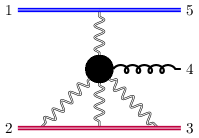
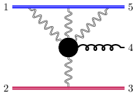
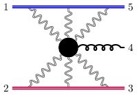
Figure 8: Schematic diagrams for multi-$W$ contributions to the $(--)$ NNLL amplitude at two-loops.

In this section we investigate NNLL predictions for the two-loop $(--)$ amplitude, which involves two-loop corrections to the $WWg$ vertex $\mathcal{W}$. At this order however, there is a significant differences with respect to the results discussed so far. Indeed, at NLL each definite-signature amplitude receives contributions from a single configuration of $W$ fields emitted from the $A$ and $B$ lines. In the case that we consider now, this is no longer true. Indeed, at NNLL the $(--)$ amplitude can be written as

$$\mathcal{A}_{{\text{NNLL}}}^{(--)}=\mathcal{A}_{{\text{NNLL}},\{1,1\}}^{(--)}+\mathcal{A}_{{\text{NNLL}},\{1,3\}}^{(--)}+\mathcal{A}_{{\text{NNLL}},\{3,1\}}^{(--)}+\mathcal{A}_{{\text{NNLL}},\{3,3\}}^{(--)},$$ (131)

where $A_{{\text{NNLL}},\{i,j\}}^{(--)}$ represents the contribution coming from a configuration with $i$ fields $W$ emitted from the $A$ line and $j$ fields $\widetilde{W}$ emitted from the $B$ line. The single-$W$ term is formally identical to the one given in eq. 125, but with the impact factors $\bar{\mathcal{J}}_{X}$ and vertex $\overline{\mathcal{W}}_{\lambda}$ expanded to two-loops and the Regge trajectory $\tau_{g}$ expanded to three loops (though the latter only enters starting from the three-loop level). Contributions involving the exchange of multiple $W$s are depicted in fig. 8. Similarly to what we discussed in section 3.2, in order to compute the full NNLL $(--)$ amplitude one should account for the rapidity evolution of the single- and triple-$W$ intermediate states. However, in analogy with the NLL case at one loop, the evolution starts at three loops so it does not affect our two-loops analysis. The computation of the multi-$W$ contributions then proceeds along lines which are very similar to the one described in section 3.2 for one-loop multi-$W$ contributions at NLL. Crucially, all the $W$ and gluon interactions can be computed at LO, thus making the calculation tedious but straightforward. Before reporting our results, however, we stress that the mixing of single- and multi-$W$ contributions makes the extraction of a universal vertex function problematic at this order. We postpone the discussion of this issue to section 4, and now focus on the calculation of the multi-$W$ terms in eq. 131.

We start by discussing the $\mathcal{A}^{(--)}_{{\text{NNLL}},\{1,3\}}$, see fig. 8. We need to consider the connected $S$-matrix contribution

$$\mathcal{S}^{(--)}_{{\text{NNLL}},\{1,3\}}=$$ (132)

$$=\phi^{[AB]}\left[2\pi\delta(p_{1}^{+}-p_{5}^{+})\delta_{\lambda_{1}\lambda_{5}}\times 2p_{1}^{+}\right]\left[2\pi\delta(p_{2}^{-}-p_{3}^{-})\delta_{\lambda_{2}\lambda_{3}}\times 2p_{2}^{-}\right]$$

$$\times\Bigg{\langle}\mathbb{T}\,\Big{(}ig_{s}\llbracket W_{\eta_{A}}({\bf q}_{A})\rrbracket_{r_{A}}\Big{)}a^{a_{4}}_{\lambda_{4}}(p_{4})\Bigg{(}\frac{(ig_{s})^{3}}{3!}\llbracket\widetilde{W}_{\eta_{B}}\otimes\widetilde{W}_{\eta_{B}}\otimes\widetilde{W}_{\eta_{B}}\rrbracket_{r_{B}}({\bf q}_{B})\Bigg{)}\Bigg{\rangle}\,=$$

$$=\phi^{[AB]}\left[2\pi\delta(p_{1}^{+}-p_{5}^{+})\delta_{\lambda_{1}\lambda_{5}}\right]\left[2\pi\delta(p_{2}^{-}-p_{3}^{-})\delta_{\lambda_{2}\lambda_{3}}\right]\times 4s_{12}\times\left[ig_{s}(T_{r_{A}}^{a})_{c_{5}c_{1}}\right]$$

$$\times g_{s}^{3}\int\{\mathrm{d}{\bf k}_{1}\}\{\mathrm{d}{\bf k}_{2}\}\Bigg{\langle}\mathbb{T}\llbracket W_{\eta_{4}}({\bf p}_{4}+{\bf q}_{A}-{\bf k}_{1})W_{\eta_{4}}({\bf k}_{1}-{\bf k}_{2})W_{\eta_{4}}({\bf k}_{2})\rrbracket^{a_{4}a}$$

$$\times\Bigg{(}\frac{(ig_{s})^{3}}{3!}\llbracket\widetilde{W}_{\eta_{B}}\otimes\widetilde{W}_{\eta_{B}}\otimes\widetilde{W}_{\eta_{B}}\rrbracket^{c_{3}c_{2}}_{r_{B}}({\bf q}_{B})\Bigg{)}\Bigg{\rangle}$$

$$\times\bigg{[}\frac{1}{6}\left(\frac{\boldsymbol{\varepsilon}^{*}_{\lambda_{4}}\cdot({\bf k}_{1}-{\bf q}_{A})}{({\bf k}_{1}-{\bf q}_{A})^{2}}\right)-\frac{1}{2}\left(\frac{\boldsymbol{\varepsilon}^{*}_{\lambda_{4}}\cdot({\bf k}_{2}-{\bf q}_{A})}{({\bf k}_{2}-{\bf q}_{A})^{2}}\right)-\frac{1}{3}\left(\frac{\boldsymbol{\varepsilon}^{*}_{\lambda_{4}}\cdot{\bf q}_{A}}{{\bf q}_{A}^{2}}\right)\bigg{]},$$

which leads to the two-loop amplitude

$$\begin{split}&\mathcal{A}_{{\text{NNLL}},\{1,3\}}^{(--)}=4g_{s}^{3}\phi^{[AB]}s_{12}\times(i\pi)^{2}\times\bigg{[}\frac{4}{3}(T^{a}_{r_{A}})_{c_{5}c_{1}}\,if^{a_{4}x_{1}c_{1}}\,if^{c_{1}x_{2}c_{2}}\,if^{c_{2}x_{3}a}\\ &\quad\times\left(T_{r_{B}}^{(x_{1}}\!\cdot\!T^{x_{2}}_{r_{B}}\!\cdot\!T^{x_{3})}_{r_{B}}\right)_{c_{3}c_{2}}\bigg{]}\times\left[\frac{g_{s}^{2}S_{\epsilon}}{(4\pi)^{2}}\right]^{2}\int\frac{\mathfrak{D}{\bf k}_{1}\mathfrak{D}{\bf k}_{2}}{{\bf k}_{2}^{2}({\bf k}_{1}-{\bf k}_{2})^{2}({\bf q}_{B}-{\bf k}_{1})^{2}}\\ &\quad\times\bigg{[}\frac{1}{6}\left(\frac{\boldsymbol{\varepsilon}^{*}_{\lambda_{4}}\cdot({\bf k}_{1}-{\bf q}_{A})}{({\bf k}_{1}-{\bf q}_{A})^{2}}\right)-\frac{1}{2}\left(\frac{\boldsymbol{\varepsilon}^{*}_{\lambda_{4}}\cdot({\bf k}_{2}-{\bf q}_{A})}{({\bf k}_{2}-{\bf q}_{A})^{2}}\right)-\frac{1}{3}\left(\frac{\boldsymbol{\varepsilon}^{*}_{\lambda_{4}}\cdot{\bf q}_{A}}{{\bf q}_{A}^{2}}\right)\bigg{]}\left(1+\mathcal{O}(\alpha_{s})\right),\end{split}$$ (133)

where $T_{r_{B}}^{(x_{1}}\!\cdot\!T^{x_{2}}_{r_{B}}\!\cdot\!T^{x_{3})}_{r_{B}}=\sum_{\sigma\in S_{3}}T_{r_{B}}^{x_{\sigma(1)}}\!\cdot\!T^{x_{\sigma(2)}}_{r_{B}}\!\cdot\!T^{x_{\sigma(3)}}_{r_{B}}$. Using the colour formalism of section 3.2, the term in the first square bracket becomes

$$\begin{split}\frac{4}{3}(T^{a}_{r_{A}})_{c_{5}c_{1}}\,&if^{a_{4}x_{1}c_{1}}\,if^{c_{1}x_{2}c_{2}}\,if^{c_{2}x_{3}a}\left(T_{r_{B}}^{(x_{1}}\!\cdot\!T^{x_{2}}_{r_{B}}\!\cdot\!T^{x_{3})}_{r_{B}}\right)_{c_{3}c_{2}}=\\ &-\left[2\boldsymbol{\mathcal{T}}_{+-}^{2}+\frac{2}{3}\boldsymbol{\mathcal{T}}_{++}^{2}+\frac{2N_{c}}{3}\boldsymbol{\mathcal{T}}_{++}\right]\left[(T_{r_{B}})_{c_{3}c_{2}}^{b}(T_{r_{A}})_{c_{5}c_{1}}^{a}if^{aba_{4}}\right],\end{split}$$ (134)

where in the rhs we have highlighted the tree-level colour structure. In doing this calculation, we have found the following Lie-algebra graphic rule useful:

$$\includegraphics[valign={m}]{tikz-fig/fig_27.pdf}-\includegraphics[valign={m}]{tikz-fig/fig_28.pdf}=-\frac{N_{c}}{2}\includegraphics[valign={m}]{tikz-fig/fig_29.pdf}.$$ (135)

Using eq. 134, we can write the two-loop result eq. 133 as

$$\mathcal{A}^{(2),(--)}_{{\text{NNLL}},\{1,3\}}=\,\pi^{2}\mathcal{K}^{(2)}_{\{1,3\}}\left[2\boldsymbol{\mathcal{T}}_{+-}^{2}+\frac{2}{3}\boldsymbol{\mathcal{T}}_{++}^{2}+\frac{2N_{c}}{3}\boldsymbol{\mathcal{T}}_{++}\right]\mathcal{A}^{(0)},$$ (136)

with

$$\begin{split}\mathcal{K}^{(2)}_{\{1,3\}}&=\left[\mathcal{K}^{(0)}_{\{1,1\}}\right]^{-1}\int\frac{\mathfrak{D}{\bf k}_{1}\mathfrak{D}{\bf k}_{2}}{{\bf k}_{2}^{2}({\bf k}_{1}-{\bf k}_{2})^{2}({\bf q}_{B}-{\bf k}_{1})^{2}}\\ &\times\bigg{[}\frac{1}{6}\left(\frac{\boldsymbol{\varepsilon}^{*}_{\lambda_{4}}\cdot({\bf k}_{1}-{\bf q}_{A})}{({\bf k}_{1}-{\bf q}_{A})^{2}}\right)-\frac{1}{2}\left(\frac{\boldsymbol{\varepsilon}^{*}_{\lambda_{4}}\cdot({\bf k}_{2}-{\bf q}_{A})}{({\bf k}_{2}-{\bf q}_{A})^{2}}\right)-\frac{1}{3}\left(\frac{\boldsymbol{\varepsilon}^{*}_{\lambda_{4}}\cdot{\bf q}_{A}}{{\bf q}_{A}^{2}}\right)\bigg{]}.\end{split}$$ (137)

Results for $\mathcal{K}^{(2)}_{\{1,3\}}$ are reported in appendix D. Here we stress that, as in the one-loop case, these functions are pure, single-valued and of uniform transcendentality. The other multi-$W$ contributions in eq. 131 can be obtained by a completely analogous procedure to what discussed in section 3.2 and above. For this reason, here we limit ourselves to presenting the final results. They read

$$\begin{split}&\mathcal{A}^{(2),(--)}_{{\text{NNLL}},\{3,1\}}=\,\pi^{2}\mathcal{K}^{(2)}_{\{3,1\}}\left[2\boldsymbol{\mathcal{T}}_{-+}^{2}+\frac{2}{3}\boldsymbol{\mathcal{T}}_{++}^{2}+\frac{2N_{c}}{3}\boldsymbol{\mathcal{T}}_{++}\right]\mathcal{A}^{(0)},\\ &\mathcal{A}^{(2),(--)}_{{\text{NNLL}},\{3,3\}}=\,-\pi^{2}\mathcal{K}^{(2)}_{\{3,3\}}\left[\frac{1}{2}\boldsymbol{\mathcal{T}}_{--}^{2}+\frac{1}{6}\boldsymbol{\mathcal{T}}_{+-}^{2}+\frac{1}{6}\boldsymbol{\mathcal{T}}_{-+}^{2}+\frac{\boldsymbol{\mathcal{T}}_{++}^{2}}{18}+\frac{2N_{c}}{9}\boldsymbol{\mathcal{T}}_{++}\right]\mathcal{A}^{(0)}.\end{split}$$ (138)

Once again, results for the $\mathcal{K}^{(2)}_{\{i,j\}}$ functions are reported in appendix D.

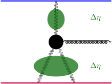
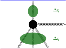
Figure 9: Examples of multi-$W$ contributions involving rapidity evolution. Diagram (a) corresponds to the all-orders NLL $\mathcal{A}^{(-+)}_{\text{NLL}}$ amplitude, diagram (b) to the all-orders $A^{(--)}_{{\text{NNLL}},\{1,3\}}$ amplitude. Similar diagrams would arise for all other transitions. The black dot stands for the leading-order vertices, while the green blobs are associated with the leading-order rapidity evolution of the $W$ states. While the evolution of a single $W$ is multiplicative and captured by the one-loop Regge trajectory ($\tau_{g}^{(1)}$), the evolution of two or more $W$s requires the computation of new 2d Feynman integrals at each perturbative order.

We conclude this section by stressing that predicting the amplitude at NNLL beyond two loops would require computing the rapidity evolution of multi-$W$ states, see fig. 9(b). As we mentioned before, these are not eigenstates of the rapidity evolution, hence this step, while not presenting conceptual challenges, would require the calculation of higher-loop 2d integrals. This is not within the scope of this paper, and we defer it to the future. We also observe that in eqs. 136 and 138 the diagonal operator $\boldsymbol{\mathcal{T}}_{++}$ generates a contribution only in the octet-octet exchange and it is leading in $N_{c}$. Indeed $\boldsymbol{\mathcal{T}}_{++}\,\mathcal{A}^{(0)}=-N_{c}/2\,\mathcal{A}^{(0)}$, irrespectively of the particle types $A$ and $B$. The non-diagonal ones, $\boldsymbol{\mathcal{T}}_{+-}^{2}$, $\boldsymbol{\mathcal{T}}_{-+}^{2}$ and $\boldsymbol{\mathcal{T}}_{--}^{2}$ have a twofold effect. First, they are responsible for a universal, representation-independent, leading-$N_{c}$ contribution in the octet-octet exchange. Second, they are the only source of colour structures different from the tree-level octet-octet one. Importantly these contributions are purely sub-leading colour, and representation dependent, i.e. they differ in quark and gluon amplitudes.

4 Results

With the results obtained so far we are ready to extract the universal vertex $\mathcal{W}$ up to two-loops. We start by collecting all shockwave amplitude predictions obtained in section 3 at the different logarithmic and perturbative orders. Comparing these results with the explicit MRK amplitudes of section 2.3 will allow us to thoroughly check the validity of our predictions in section 3 at NLL and determine for the first time the two-loop QCD contribution to the $WWg$ vertex. The $2\to 3$ MRK amplitudes computed in ref. Caron-Huot:2020vlo will also allow us to compute the same quantity in $\mathcal{N}=4$ super Yang–Mills theory, and explicitly verify the maximal transcendentality principle in this context.

The main results of this publication are also distributed through the ancillary files of this publication. All results in electronic format are also available at results:url . The interested reader will find a README file with a detailed explanation of their content and the notation adopted.

4.1 Summary and extraction of the gluon emission vertex

At tree level the only contribution which corresponds to LL accuracy comes from the single–$W$ amplitude in eq. 94, which yields

$$\mathcal{A}^{(0)}_{\text{LL}} ={\includegraphics[valign={m}]{tikz-fig/fig_32.pdf}}=\mathcal{A}^{(0)}.$$ (139)

At one-loop one has instead

$$\mathcal{A}^{(1)}_{\text{LL}} ={\includegraphics[valign={m}]{tikz-fig/fig_33.pdf}}+{\includegraphics[valign={m}]{tikz-fig/fig_34.pdf}}=\left[L_{A}\tau_{A}^{(1)}+L_{B}\tau_{B}^{(1)}\right]\mathcal{A}^{(0)},$$ (140)

$$\mathcal{A}^{(1),(--)}_{\text{NLL}} ={\includegraphics[valign={m}]{tikz-fig/fig_35.pdf}}+{\includegraphics[valign={m}]{tikz-fig/fig_36.pdf}}+{\includegraphics[valign={m}]{tikz-fig/fig_37.pdf}}=\left[\bar{\mathcal{J}}_{A}^{(1)}+\bar{\mathcal{J}}_{B}^{(1)}+\overline{\mathcal{W}}_{\lambda_{4}}^{(1)}\right]\mathcal{A}^{(0)},$$ (141)

$$\mathcal{A}^{(1),(+-)}_{\text{NLL}} ={\includegraphics[valign={m}]{tikz-fig/fig_38.pdf}}=i\pi B^{(1)}_{-+}\boldsymbol{\mathcal{T}}_{-+}\mathcal{A}^{(0)},$$ (142)

$$\mathcal{A}^{(1),(-+)}_{\text{NLL}} ={\includegraphics[valign={m}]{tikz-fig/fig_39.pdf}}=i\pi B^{(1)}_{+-}\boldsymbol{\mathcal{T}}_{+-}\mathcal{A}^{(0)},$$ (143)

$$\mathcal{A}^{(1),(++)}_{\text{NLL}} ={\includegraphics[valign={m}]{tikz-fig/fig_40.pdf}}=i\pi B^{(1)}_{--}\boldsymbol{\mathcal{T}}_{--}\mathcal{A}^{(0)},$$ (144)

where we introduced the multi-$W$ coefficients

$$B^{(1)}_{-+}=-\mathcal{K}^{(1)}_{\{2,1\}},\quad\quad B^{(1)}_{+-}=-\mathcal{K}^{(1)}_{\{1,2\}},\quad\quad B^{(1)}_{--}=-\mathcal{K}^{(1)}_{\{2,2\}}.$$ (145)

In eq. 140 $\tau^{(1)}_{A,B}$ is the one-loop Regge trajectory given by eqs. 88 and 118, whereas $\bar{\mathcal{J}}^{(1)}_{A,B}$ and $\overline{\mathcal{W}}_{\lambda_{4}}^{(1)}$ in eq. 141 are, respectively, the impact factors and the central-emission vertex at one-loop accuracy.

We stress that the formulas given so far provide a complete prediction of the one-loop MRK amplitude, i.e. for all possible signatures. Moreover, the expressions are universal across all partonic channels, with the only representation-dependent components being the impact factors $\bar{\mathcal{J}}_{X}$, and the effect of the non-diagonal colour operators. We report the explicit result of the action of such colour operators on the tree-level amplitude for the various partonic channels in appendix B.

At two loops we restrict our attention to the odd-odd part of the amplitude where the various logarithmic orders read

$$\mathcal{A}^{(2)}_{\text{LL}} ={\includegraphics[valign={m}]{tikz-fig/fig_49.pdf}}+{\includegraphics[valign={m}]{tikz-fig/fig_50.pdf}}+{\includegraphics[valign={m}]{tikz-fig/fig_51.pdf}}=\frac{1}{2}(L_{A}\tau_{A}^{(1)}+L_{B}\tau_{B}^{(1)})^{2}\mathcal{A}^{(0)},$$ (146)

$$\mathcal{A}^{(2),(--)}_{\text{NLL}} ={\includegraphics[valign={m}]{tikz-fig/fig_52.pdf}}+{\includegraphics[valign={m}]{tikz-fig/fig_53.pdf}}+{\includegraphics[valign={m}]{tikz-fig/fig_54.pdf}}+{\includegraphics[valign={m}]{tikz-fig/fig_55.pdf}}$$

$$+{\includegraphics[valign={m}]{tikz-fig/fig_56.pdf}}+{\includegraphics[valign={m}]{tikz-fig/fig_57.pdf}}+{\includegraphics[valign={m}]{tikz-fig/fig_58.pdf}}+{\includegraphics[valign={m}]{tikz-fig/fig_59.pdf}}$$ (147)

$$=\Big{[}(L_{A}\tau_{A}^{(2)}+L_{B}\tau_{B}^{(2)})+(L_{A}\tau_{A}^{(1)}+L_{B}\tau_{B}^{(1)})(\bar{\mathcal{J}}_{A}^{(1)}+\bar{\mathcal{J}}_{B}^{(1)}+\overline{\mathcal{W}}_{\lambda_{4}}^{(1)})\Big{]}\mathcal{A}^{(0)},$$

$$\mathcal{A}^{(2),(--)}_{{\text{NNLL}}} ={\includegraphics[valign={m}]{tikz-fig/fig_60.pdf}}+{\includegraphics[valign={m}]{tikz-fig/fig_61.pdf}}+{\includegraphics[valign={m}]{tikz-fig/fig_62.pdf}}+{\includegraphics[valign={m}]{tikz-fig/fig_63.pdf}}+$$

$$+{\includegraphics[valign={m}]{tikz-fig/fig_64.pdf}}+{\includegraphics[valign={m}]{tikz-fig/fig_65.pdf}}+{\includegraphics[valign={m}]{tikz-fig/fig_66.pdf}}+{\includegraphics[valign={m}]{tikz-fig/fig_67.pdf}}+{\includegraphics[valign={m}]{tikz-fig/fig_68.pdf}}$$ (148)

$$=\Bigg{[}\overline{\mathcal{W}}^{(2)}_{\lambda_{4}}+\bar{\mathcal{J}}_{A}^{(2)}+\bar{\mathcal{J}}_{B}^{(2)}+\bar{\mathcal{J}}_{A}^{(1)}\bar{\mathcal{J}}_{B}^{(1)}+\overline{\mathcal{W}}_{\lambda_{4}}^{(1)}(\bar{\mathcal{J}}_{A}^{(1)}+\bar{\mathcal{J}}_{B}^{(1)})$$

$$\quad\quad+(i\pi)^{2}\Big{(}B^{(2)}_{+-}\boldsymbol{\mathcal{T}}_{+-}^{2}+B^{(2)}_{--}\boldsymbol{\mathcal{T}}_{--}^{2}+B^{(2)}_{-+}\boldsymbol{\mathcal{T}}_{-+}^{2}-B^{(2)}_{d}\frac{N_{c}^{2}}{4}\Big{)}\Bigg{]}\mathcal{A}^{(0)}.$$

The multi-$W$ kinematic coefficients at the two-loop level are

$$\begin{gathered}B^{(2)}_{+-}=-2\mathcal{K}^{(2)}_{\{1,3\}}+\frac{\mathcal{K}^{(2)}_{\{3,3\}}}{6},\quad\quad B^{(2)}_{-+}=-2\mathcal{K}^{(2)}_{\{3,1\}}+\frac{\mathcal{K}^{(2)}_{\{3,3\}}}{6},\quad\quad B^{(2)}_{--}=\frac{\mathcal{K}^{(2)}_{\{3,3\}}}{2},\\ B^{(2)}_{d}=-\frac{2}{3}\left(\mathcal{K}^{(2)}_{\{1,3\}}+\mathcal{K}^{(2)}_{\{3,1\}}\right)+\frac{7}{18}\mathcal{K}^{(2)}_{\{3,3\}}.\end{gathered}$$ (149)

We point out that the contributions from the diagonal operators $\boldsymbol{\mathcal{T}}_{++}$ and $\boldsymbol{\mathcal{T}}^{2}_{++}$ appearing in eqs. 136 and 138 have been absorbed in the coefficient $B^{(2)}_{d}$. As in the one-loop case, the superscript $(2)$ refers to two-loop corrections to the MRK building blocks.

We now outline our approach for the extraction of the universal coefficients $\overline{\mathcal{W}}^{(1)}$ and $\overline{\mathcal{W}}^{(2)}$. While the former is already present in the literature, the latter is in fact unknown. We begin by noting that by using the Balitsky-JIMWLK formalism, the Regge trajectory as well as the quark and gluon impact factors can be extracted by studying the Regge limit of $2\to 2$ scattering amplitudes. Because of this we will regard $\tau_{g}^{(\ell)}$ and $\bar{\mathcal{J}}_{X}^{(\ell)}$ as known quantities. Starting at LL accuracy, the only relevant contribution is the LO gluon Regge trajectory. It is straightforward to check that eqs. 140 and 146, combined with eq. 88, indeed match the amplitudes computed in section 2.3 at this logarithmic order.

At NLL, the prediction for the odd-odd component includes for the first time a perturbative correction to the impact factors and to the $WWg$ vertex $\overline{\mathcal{W}}_{\lambda}$. We can then extract $\overline{\mathcal{W}}^{(1)}$ from eq. 141, by matching with the one-loop MRK amplitudes obtained in section 2.3. This was indeed the procedure followed in ref. DelDuca:1998cx to obtain the one-loop corrections to the Lipatov vertex at $\mathcal{O}(\epsilon^{0})$. In addition, we can now fully predict the two-loop NLL odd-odd component $\mathcal{A}^{(2),(--)}_{\text{NLL}}$ via eq. 147, which serves as a strong check of the formalism up to this logarithmic accuracy. As far as the components involving even signatures are concerned, there are no unknown quantities involved, thus no matching to explicit amplitudes is required and eqs. (142), (143) and (144) directly reproduce the results obtained in section 2.3. Taking into account the various ingredients described above, we find full agreement.

Finally, at NNLL we focus on the odd-odd amplitude, which receives contributions from various effects: the two-loop impact factors $\bar{\mathcal{J}}^{(2)}_{X}$, the two-loop correction to $\overline{\mathcal{W}}$ and the $W\to 3W$, $3W\to W$ and $3W\to 3W$ transitions. Our direct calculation of the multi-$W$ coefficients $B^{(2)}_{\sigma_{1},\sigma_{2}}$ then leaves only $\overline{\mathcal{W}}^{(2)}$ undetermined and allows us to compute it by matching the corresponding explicit UV-renormalised MRK amplitude.

4.2 Collecting the universal contributions

The results obtained in the previous section are consistent with the effective approach described in section 3. However, we point out again that the multi-$W$ contributions found at NNLL contain universal leading-$N_{c}$ terms in the octet-octet colour channel. In particular, at large $N_{c}$

$$\boldsymbol{\mathcal{T}}_{-+}^{2}\approx\boldsymbol{\mathcal{T}}_{+-}^{2}\approx\boldsymbol{\mathcal{T}}_{--}^{2}\approx\frac{N_{c}^{2}}{4},$$ (150)

so we find that in leading-colour approximation the multi-$W$ contributions are given by

$${\includegraphics[valign={m}]{tikz-fig/fig_66.pdf}}\!+\!{\includegraphics[valign={m}]{tikz-fig/fig_67.pdf}}\!+\!{\includegraphics[valign={m}]{tikz-fig/fig_68.pdf}}\approx(i\pi)^{2}\frac{N_{c}^{2}}{4}\Big{(}B^{(2)}_{+-}\!+\!B^{(2)}_{--}\!+\!B^{(2)}_{-+}\!-\!B^{(2)}_{d}\Big{)}\mathcal{A}^{(0)}.$$ (151)

Therefore, the only part which distinguishes between the representations of the projectiles is given by the sub-leading $N_{c}$ coefficients in the multi-$W$ exchanges.

As discussed in ref. Falcioni:2021dgr , it is natural to isolate the universal components of the multi-$W$ interactions and reabsorb it into a redefinition of the radiative corrections of the single-$W$ amplitude. For consistency, this has to be done both for the $2\to 2$ and for $2\to 3$ amplitudes. In the $2\to 2$ case this amounts to defining new impact factors and Regge-trajectory so that up to NNLL

$$\mathcal{A}_{2\to 2,{\text{NNLL}}}^{(--)}=\mathcal{I}_{A}e^{\tau_{s}L_{s}}\cos\left(\frac{\pi\tau_{s}}{2}\right)\mathcal{I}_{B}\times\mathcal{A}_{2\to 2}^{(0)}+[\text{multi $W$ exchanges}]_{\mathrm{SLC}}.$$ (152)

While up to two-loops the Regge trajectory remains unchanged (hence the slight abuse of notation in the equation above), the $\mathcal{O}(\alpha_{s}^{2})$ correction to the impact factors is modified with respect to the one in section 3. It is straightforward to obtain the new impact factors $\mathcal{I}_{X}$ from the results of ref. Falcioni:2021dgr , after having taken into account the additional cosine factor in the factorisation formula (152). The explicit formulae for these impact factors are given in the ancillary files.

Coming to the $2\to 3$ case, we define a modified $WWg$ vertex coefficient $\mathcal{U}_{\lambda}$, which up to two loops reads

$${\mathcal{U}}_{\lambda}^{(0)}=1,\quad{\mathcal{U}}_{\lambda}^{(1)}=\overline{\mathcal{W}}^{(1)}_{\lambda},\quad{\mathcal{U}}_{\lambda}^{(2)}=\overline{\mathcal{W}}^{(2)}_{\lambda}+\frac{N_{c}^{2}}{4}\left(B^{(2)}_{+-}+B^{(2)}_{--}+B^{(2)}_{-+}-B^{(2)}_{d}\right).$$ (153)

This allows us to rewrite the NNLL odd-odd amplitude prediction as follows:

$$\mathcal{A}^{(2),(--)}_{{\text{NNLL}}}=\Bigg{\{}\mathcal{U}_{{\lambda_{4}}}^{(2)}+\mathcal{I}_{A}{}^{(2)}+\mathcal{I}_{B}{}^{(2)}+\mathcal{I}_{A}{}^{(1)}\mathcal{I}_{B}{}^{(1)}+\mathcal{U}_{{\lambda_{4}}}^{(1)}(\mathcal{I}_{A}{}^{(1)}+\mathcal{I}_{B}{}^{(1)})$$ (154)

$$+(i\pi)^{2}\Bigg{[}B^{(2)}_{+-}\left(\boldsymbol{\mathcal{T}}_{+-}^{2}\!-\!\frac{N_{c}^{2}}{4}\right)+B^{(2)}_{--}\left(\boldsymbol{\mathcal{T}}_{--}^{2}\!-\!\frac{N_{c}^{2}}{4}\right)+B^{(2)}_{-+}\left(\boldsymbol{\mathcal{T}}_{-+}^{2}\!-\!\frac{N_{c}^{2}}{4}\right)\Bigg{]}\Bigg{\}}\mathcal{A}^{(0)},$$

where the first line contains all universal contributions while the second one is manifestly sub-leading-colour. In the following sections, we will present our results in terms of the universal coefficient $\mathcal{U}$.

Before presenting any result, we point out that, since we are working with UV-renormalised amplitudes, the vertex corrections ${\mathcal{U}}^{(1)}_{\lambda}$ and ${\mathcal{U}}^{(2)}_{\lambda}$ obtained from the procedure above still contain IR poles and are regularisation scheme dependent. Furthermore they are affected by spurious kinematic singularities which obscure their simplicity. For these reasons, we find it convenient to express our results in terms of finite remainders, which we define in the next section. We will see that, in addition to being free of IR poles, they are also free of spurious singularities when expressed in terms of the single-valued functions defined in section 2.4. This is to be expected since the same properties are seen in the finite amplitudes defined in section 2.3.

4.3 Finite remainders

In order to define finite remainders for the various building blocks of MRK factorisation, we look more closely at the IR anomalous dimension eq. 42. We highlight the different contributions by rewriting it as follows

$${\bf\Gamma}_{IR} =\gamma_{K}\mathcal{C}_{A}\ln\frac{-s_{51}}{\mu^{2}}-\frac{\gamma_{K}}{2}\ln\frac{-s_{51}}{\rho^{2}}({\bf T}^{15}_{+})^{2}+2\gamma_{A}$$ (155)

$$+\gamma_{K}\mathcal{C}_{B}\ln\frac{-s_{23}}{\mu^{2}}-\frac{\gamma_{K}}{2}\ln\frac{-s_{23}}{\rho^{2}}({\bf T}^{23}_{+})^{2}+2\gamma_{B}$$

$$+\gamma_{K}L_{A}({\bf T}^{15}_{+})^{2}+\gamma_{K}L_{B}({\bf T}^{23}_{+})^{2}$$

$$+\frac{\gamma_{K}}{2}\left(-\mathcal{C}_{4}\ln\frac{\mu^{2}}{{\bf p}_{4}^{2}}+\ln\frac{\rho^{2}}{{\bf p}_{4}^{2}}({\bf T}^{15}_{+})^{2}+\ln\frac{\rho^{2}}{{\bf p}_{4}^{2}}({\bf T}^{23}_{+})^{2}-i\pi\,\boldsymbol{\mathcal{T}}_{++}\right)+\gamma_{4}$$

$$+\frac{\gamma_{K}}{2}\times i\pi\left(\boldsymbol{\mathcal{T}}_{+-}+\boldsymbol{\mathcal{T}}_{--}+\boldsymbol{\mathcal{T}}_{-+}\right).$$

The first two lines contain the collinear and soft singularities of the projectiles; these are the only terms that depend on the particle types $A$ and $B$. The third line is the only source of large logarithms and is therefore associated with the rapidity evolutions in the $s_{51}$ and $s_{23}$ channels. The fourth lines captures the dependence on the central gluon momentum, colour charge and collinear anomalous dimension and can therefore be associated with the $WWg$ interaction, at least at one loop. Finally, the fifth line contains the only non-diagonal and signature mixing operators and is purely imaginary, thus it is connected with the multi–$W$ exchange contributions.

We can then proceed by writing the IR renormalisation matrix as

$${\bf Z}_{IR}=\exp\left({\boldsymbol{\zeta}}_{A}+{\boldsymbol{\zeta}}_{B}+{\boldsymbol{\zeta}}_{\tau_{A}}+{\boldsymbol{\zeta}}_{\tau_{B}}+{\boldsymbol{\zeta}}_{+}+{\boldsymbol{\zeta}}_{-}\right),$$ (156)

where the quantities in the exponent correspond to the different components of eq. 155 after the scale integration of eq. 41 has been carried out. Explicitly they read

$${\boldsymbol{\zeta}}_{A}=K\left(\mathcal{C}_{A}\ln\frac{-s_{51}}{\mu^{2}}-\frac{1}{2}\ln\frac{-s_{51}}{\rho^{2}}({\bf T}^{15}_{+})^{2}\right)+2G_{A}-2K^{\prime}\mathcal{C}_{A},$$

$${\boldsymbol{\zeta}}_{B}=K\left(\mathcal{C}_{B}\ln\frac{-s_{23}}{\mu^{2}}-\frac{1}{2}\ln\frac{-s_{23}}{\rho^{2}}({\bf T}^{23}_{+})^{2}\right)+2G_{B}-2K^{\prime}\mathcal{C}_{B},$$

$${\boldsymbol{\zeta}}_{\tau_{A}}=KL_{A}({\bf T}^{15}_{+})^{2},\quad{\boldsymbol{\zeta}}_{\tau_{B}}=KL_{B}({\bf T}^{23}_{+})^{2},$$ (157)

$${\boldsymbol{\zeta}}_{-}=\frac{i\pi}{2}K\left(\boldsymbol{\mathcal{T}}_{+-}+\boldsymbol{\mathcal{T}}_{--}+\boldsymbol{\mathcal{T}}_{-+}\right),$$

$${\boldsymbol{\zeta}}_{+}=\frac{K}{2}\Big{[}-\mathcal{C}_{4}\ln\frac{\mu^{2}}{{\bf p}_{4}^{2}}+\ln\frac{\rho^{2}}{{\bf p}_{4}^{2}}({\bf T}^{15}_{+})^{2}+\ln\frac{\rho^{2}}{{\bf p}_{4}^{2}}({\bf T}^{23}_{+})^{2}-i\pi\,\boldsymbol{\mathcal{T}}_{++}\Big{]}+G_{4}-K^{\prime}\mathcal{C}_{4},$$

with the additional definitions

$$K=\int_{\mu}^{\infty}\frac{d\lambda}{\lambda}\gamma_{K}(\alpha(\lambda)),\quad K^{\prime}=\int_{\mu}^{\infty}\frac{d\lambda}{\lambda}K(\alpha(\lambda)),\quad G_{i}=\int_{\mu}^{\infty}\frac{d\lambda}{\lambda}\gamma_{i}(\alpha(\lambda)),$$ (158)

whose perturbative expansions up to the required order are given in appendix C.

We now get to the definition of finite remainders for the various building blocks of MRK factorisation. We start from the Regge trajectory and impact factors. Based on the results of ref. Falcioni:2021buo , we know that, at least up to two loops, the quantities

$$\hat{\tau}_{g}({\bf q})={\tau_{g}}({\bf q})-KN_{c},\quad\quad\hat{\mathcal{I}}_{X}({\bf q})=e^{-\zeta_{X}}\mathcal{I}_{X}({\bf p})$$ (159)

are finite. The finite corrections to the Regge trajectory read

$$\hat{\tau}^{(1)}({\bf q};\mu) =2N_{c}\ln\left(\frac{\mu^{2}}{{\bf q}^{2}}\right),$$ (160)

$$\hat{\tau}^{(2)}({\bf q};\mu) =N_{c}\left[\beta_{0}\,\ln^{2}\left(\frac{\mu^{2}}{{\bf q}^{2}}\right)+\frac{\gamma_{K}^{(2)}}{2}\ln\left(\frac{\mu^{2}}{{\bf q}^{2}}\right)+N_{c}\left(\frac{404}{27}-2\zeta_{3}\right)-\frac{56}{27}N_{f}\right]\,.$$ (161)

The perturbative coefficients of the impact factors instead are

$$\hat{\mathcal{I}}_{g}^{(1)} =\left(4\zeta_{2}-\frac{67}{18}\right)N_{c}+\frac{5N_{f}}{9},$$ (162)

$$\hat{\mathcal{I}}_{q}^{(1)} =\left(\frac{13}{18}+\frac{7\zeta_{2}}{2}\right)N_{c}+\frac{8-\zeta_{2}}{2N_{c}}-\frac{5N_{f}}{9},$$ (163)

$$\hat{\mathcal{I}}_{g}^{(2)} =\left(\frac{88\zeta_{3}}{9}-\frac{3\zeta_{4}}{2}+\frac{335\zeta_{2}}{18}-\frac{26675}{648}\right)N_{c}^{2}+\left(\frac{2\zeta_{3}}{9}-\frac{25\zeta_{2}}{9}+\frac{2063}{216}\right)N_{c}N_{f}$$

$$-\frac{25N_{f}^{2}}{162}+\left(2\zeta_{3}-\frac{55}{24}\right)\frac{N_{f}}{N_{c}},$$ (164)

$$\hat{\mathcal{I}}_{q}^{(2)} =\left(\frac{41\zeta_{3}}{9}-\frac{35\zeta_{4}}{16}+\frac{87\zeta_{2}}{4}+\frac{22537}{2592}\right)N_{c}^{2}-\left(\frac{23\zeta_{3}}{9}+4\zeta_{2}+\frac{650}{81}\right)N_{c}N_{f}$$

$$+\frac{25N_{f}^{2}}{54}-\left(\frac{19\zeta_{3}}{9}+\zeta_{2}+\frac{505}{81}\right)\frac{N_{f}}{N_{c}}-\frac{205\zeta_{3}}{18}-\frac{47\zeta_{4}}{8}+\frac{19\zeta_{2}}{2}+\frac{28787}{648}$$

$$+\left(-\frac{15\zeta_{3}}{2}-\frac{83\zeta_{4}}{16}+\frac{21\zeta_{2}}{4}+\frac{255}{32}\right)\frac{1}{N_{c}^{2}}.$$ (165)

where we set the renormalisation and factorisation scales to $\mu^{2}=\rho^{2}={\bf q}^{2}$. We provide results for generic scales as well as their UV renormalised counterparts in the ancillary files of this publication.

We now move to the determination of finite remainders for the cut coefficients and the $WWg$ vertex. Our strategy to do so consists in defining a finite scattering amplitude

$$\mathcal{F}=\lim_{\epsilon\to 0}\,\mathbf{Z}_{IR}^{-1}\,{\mathcal{A}},$$ (166)

inserting the formal expressions of eqs. (139)—(144), (146)—(147) and (154) into $\mathcal{A}$ and writing the Regge trajectory and the impact factors in terms of their finite remainders in eq. 159. We then compare the various signature components on the two sides of the equation at different logarithmic and perturbative orders. Since the components of $\mathcal{F}$ are finite we can simply read off the finite remainders for $B_{\sigma_{1},\sigma_{2}}^{(\ell)}$ and $\mathcal{U}$. We now describe in detail how we do this.

Starting from the one- and two-loop LL amplitudes, we simply find

$$\mathcal{F}^{(1),(--)}_{\mathrm{LL}}=\left[L_{A}\hat{\tau}_{A}^{(1)}+L_{B}\hat{\tau}_{B}^{(1)}\right]\mathcal{A}^{(0)},\quad\quad\mathcal{F}^{(2),(--)}_{\mathrm{LL}}=\frac{1}{2}\left[L_{A}\hat{\tau}_{A}^{(1)}+L_{B}\hat{\tau}_{B}^{(1)}\right]^{2}\mathcal{A}^{(0)},$$ (167)

which is consistent with the finiteness of $\hat{\tau}_{g}$ and does not provide any further information. Moving to NLL, the odd-odd one-loop component reads

$$\mathcal{F}^{(1),(--)}_{\mathrm{NLL}}=\left[\hat{\mathcal{I}}_{A}^{(1)}+\hat{\mathcal{I}}_{B}^{(1)}+\left(\mathcal{U}^{(1)}_{\lambda_{4}}-{\boldsymbol{\zeta}}_{+}^{(1)}\right)\right]\mathcal{A}^{(0)},$$ (168)

so that the one-loop finite remainder for the vertex is given by

$$\hat{\mathcal{U}}^{(1)}_{\lambda}=\mathcal{U}^{(1)}_{\lambda}-\zeta_{+}^{(1)},$$ (169)

where $\zeta_{+}$ is defined (at all orders) as the eigenvalue ${\boldsymbol{\zeta}}_{+}\mathcal{A}^{(0)}=\zeta_{+}\mathcal{A}^{(0)}$. Moving to components involving even signatures, we get

$$\begin{split}\mathcal{F}^{(1),(-+)}_{\text{NLL}}=i\pi(B^{(1)}_{+-}-\frac{K^{(1)}}{2})\boldsymbol{\mathcal{T}}_{+-}\mathcal{A}^{(0)},\\ \mathcal{F}^{(1),(+-)}_{\text{NLL}}=i\pi(B^{(1)}_{-+}-\frac{K^{(1)}}{2})\boldsymbol{\mathcal{T}}_{-+}\mathcal{A}^{(0)},\\ \mathcal{F}^{(1),(++)}_{\text{NLL}}=i\pi(B^{(1)}_{--}-\frac{K^{(1)}}{2})\boldsymbol{\mathcal{T}}_{--}\mathcal{A}^{(0)},\end{split}$$ (170)

which prompts us to define the finite remainders for the one-loop multi-$W$ coefficients as

$$\hat{B}^{(1)}_{\sigma_{1}\sigma_{2}}=B^{(1)}_{\sigma_{1}\sigma_{2}}-\frac{K^{(1)}}{2}.$$ (171)

Finally, at NNLL we organise the odd-odd two-loop amplitude according to its colour structure and find:

$$\mathcal{F}^{(2),(--)}_{{\text{NNLL}}}=\Bigg{\{}\hat{\mathcal{U}}_{{\lambda_{4}}}^{(2)}+\hat{\mathcal{I}}_{A}{}^{(2)}+\hat{\mathcal{I}}_{B}{}^{(2)}+\hat{\mathcal{I}}_{A}{}^{(1)}\hat{\mathcal{I}}_{B}{}^{(1)}+\hat{\mathcal{U}}_{{\lambda_{4}}}^{(1)}(\hat{\mathcal{I}}_{A}{}^{(1)}+\hat{\mathcal{I}}_{B}{}^{(1)})$$ (172)

$$+(i\pi)^{2}\Bigg{[}\hat{B}^{(2)}_{+-}\left(\boldsymbol{\mathcal{T}}_{+-}^{2}\!-\!\frac{N_{c}^{2}}{4}\right)+\hat{B}^{(2)}_{--}\left(\boldsymbol{\mathcal{T}}_{--}^{2}\!-\!\frac{N_{c}^{2}}{4}\right)+\hat{B}^{(2)}_{-+}\left(\boldsymbol{\mathcal{T}}_{-+}^{2}\!-\!\frac{N_{c}^{2}}{4}\right)\Bigg{]}\Bigg{\}}\mathcal{A}^{(0)},$$

where we have defined the finite remainders for two-loop vertex correction and the two-loop multi-$W$ coefficients as

$$\hat{\mathcal{U}}^{(2)}_{\lambda_{4}} =\mathcal{U}^{(2)}-\zeta_{+}^{(1)}\mathcal{U}^{(1)}+\frac{1}{2}(\zeta_{+}^{(1)})^{2}-\zeta_{+}^{(2)}$$ (173)

$$\quad\quad-(i\pi)^{2}\frac{N_{c}^{2}}{4}\left(\frac{K^{(1)}}{2}(B^{(1)}_{+-}+B^{(1)}_{-+}+B^{(1)}_{--})-\frac{3}{8}(K^{(1)})^{2}\right),$$

$$\hat{B}^{(2)}_{\sigma_{1}\sigma_{2}} =B^{(2)}_{\sigma_{1}\sigma_{2}}-\frac{K^{(1)}}{2}B^{(1)}_{\sigma_{1}\sigma_{2}}+\frac{1}{8}(K^{(1)})^{2}.$$

In particular, the subtraction of the leading-colour terms from the operators $\boldsymbol{\mathcal{T}}^{2}_{\sigma_{1}\sigma_{2}}$ arising from the definition eq. 154 causes the appearance of the second line in of the definition of $\hat{\mathcal{U}}^{(2)}$.

We highlight the fact that, thanks to our definition of the finite remainders $\hat{\tau}$, $\hat{\mathcal{I}}_{X}$, $\hat{\mathcal{U}}$ and $\hat{B}^{(\ell)}_{\sigma_{1}\sigma_{2}}$, the finite amplitude has exactly the same MRK-factorised form of the UV renormalised one. In other words, the components of the finite amplitude can be obtained by replacing each quantity in eqs. (139)—(144), (146)—(147) and (154) by its corresponding finite remainder, as defined above. In principle this allows us to perform the extraction of the finite quantities directly from $\mathcal{F}$, without ever working with the UV-renormalised but still IR-divergent amplitude $\mathcal{A}$.

4.4 Finite results in QCD and $\mathcal{N}=4$ sYM

We now present our results for the $WWg$ vertex coefficient in QCD and $\mathcal{N}=4$ sYM. In particular we provide the one- and two-loop corrections, which enter at NNLL accuracy in the MRK regime. While reminding the reader of the perturbative expansion

$$\hat{\mathcal{U}}_{\lambda_{4}}=1+\left(\frac{\alpha_{s}}{4\pi}\right)\hat{\mathcal{U}}_{\lambda_{4}}^{(1)}+\left(\frac{\alpha_{s}}{4\pi}\right)^{2}\hat{\mathcal{U}}_{\lambda_{4}}^{(2)}+\dots\,,$$ (174)

we note that one-loop correction is not new, however we report its finite remainder here for completeness. The two-loop term instead appears here for the first time. We present both written in terms of the single-valued functions $h_{i,j}$ and the rational functions $r_{i}$ defined in section 2.3.

The QCD results are

$$\hat{\mathcal{U}} {}_{+,QCD}^{(1)}=\frac{N_{c}}{2}\left(5\zeta_{2}-h_{1,2}\left(h_{1,2}+3r_{3}\right)-i\pi h_{1,1}\right)-\frac{N_{c}-N_{f}}{3}\left(r_{1}h_{1,2}+r_{2}\right),$$ (175)

$$\hat{\mathcal{U}} {}_{+,QCD}^{(2)}=N_{c}^{2}\Bigg{[}\frac{1}{144}i\pi\bigg{(}-72\zeta_{3}+h_{1,1}\left(-36\zeta_{2}+9h_{1,2}\left(3r_{3}+4h_{1,2}\right)-456\right)+464$$

$$\quad\quad-27r_{3}\left(h_{1,3}h_{1,4}+8h_{2,2}-8h_{2,3}\right)\bigg{)}+\frac{1}{432}\bigg{(}216r_{2}-1809\zeta_{4}+216r_{1}h_{1,2}-2872$$

$$\quad\quad+36\zeta_{2}\left(-18h_{1,1}^{2}+3\left(9r_{3}-7h_{1,2}\right)h_{1,2}+209\right)-9\big{(}-6h_{1,2}^{4}+98h_{1,2}^{2}+9r_{3}\big{(}2h_{1,2}^{3}$$

$$\quad\quad+3\left(\left(h_{1,1}-4\right)h_{1,1}+24\right)h_{1,2}+h_{1,1}\left(h_{1,3}h_{1,4}+8h_{2,2}-8h_{2,3}\right)+64h_{3,6}\big{)}\big{)}\bigg{)}\Bigg{]}$$

$$+N_{c}\left(N_{c}-N_{f}\right)\Bigg{[}\frac{1}{216}i\pi\bigg{(}36r_{4}+36r_{2}\left(h_{1,1}-1\right)+108r_{3}h_{1,2}+3h_{1,1}\left(3r_{1}h_{1,2}-40\right)$$

$$\quad\quad-9r_{1}\left(12h_{1,2}+h_{1,3}h_{1,4}+8h_{2,2}-8h_{2,3}\right)+112\bigg{)}+\frac{1}{648}\bigg{(}36\zeta_{2}\left(9r_{1}h_{1,2}+55\right)$$

$$\quad\quad+36\left(3\left(5r_{3}+r_{6}\right)-113r_{1}\right)h_{1,2}+36r_{2}\left(3h_{1,2}^{2}-15\zeta_{2}+6h_{1,1}-137\right)-9\big{(}9r_{1}h_{1,2}h_{1,1}^{2}$$

$$\quad\quad-3\big{(}4r_{4}-12r_{3}h_{1,2}+r_{1}\left(36h_{1,2}-h_{1,3}h_{1,4}-8h_{2,2}+8h_{2,3}\right)-4\big{)}h_{1,1}+2\big{(}3r_{1}h_{1,2}^{3}$$

$$\quad\quad+\left(6r_{5}+2\right)h_{1,2}^{2}-18\left(r_{1}-r_{3}\right)\left(h_{1,3}h_{1,4}+8h_{2,2}-8h_{2,3}\right)+96r_{1}h_{3,6}\big{)}\big{)}-260\bigg{)}\Bigg{]}$$

$$+N_{c}\beta^{\text{(0)}}\Bigg{[}\frac{1}{8}i\pi\bigg{(}h_{1,1}^{2}+2h_{1,2}^{2}+4\zeta_{2}-8h_{2,1}\bigg{)}+\frac{1}{48}\bigg{(}-h_{1,4}^{3}-3h_{1,1}^{2}h_{1,4}+3h_{1,2}^{2}h_{1,4}$$

$$\quad\quad-9h_{1,2}\left(h_{1,3}h_{1,4}+8h_{2,2}-8h_{2,3}\right)-48\left(2\zeta_{2}h_{1,4}-2h_{3,4}+2h_{3,5}+h_{3,7}\right)$$

$$\quad\quad+3h_{1,3}^{2}h_{1,4}+232\zeta_{3}+3h_{1,1}\left(5h_{1,2}^{2}+2h_{1,3}h_{1,2}-16h_{2,1}\right)\bigg{)}\Bigg{]}$$

$$+\frac{\left(N_{c}-N_{f}\right){}^{2}}{54}\!\Bigg{[}\left(r_{2}\!+\!r_{1}h_{1,2}\right)\left(6h_{1,1}\!-\!20\right)+3h_{1,2}h_{1,2}\Bigg{]}\!+\!\frac{N_{f}}{2N_{c}}\!\Bigg{[}r_{2}+\left(r_{1}\!-\!2r_{3}\right)h_{1,2}\Bigg{]},$$ (176)

where we have set $\mu^{2}=\rho^{2}={\bf p}_{4}^{2}$ and selected the $\lambda_{4}=+1$ helicity of the emitted gluon. The vertex coefficients for $\lambda_{4}=-1$ can be obtained by simply swapping $z\leftrightarrow\bar{z}$ in the equations above. The results with full dependence on the scales $\mu$ and $\rho$, as well as the higher orders in $\epsilon$ of the one-loop correction, are given in the ancillary files.

Two comments are now in order:

• the one-loop result is purely leading colour. The two-loop correction is also leading colour, except for a sub-leading $N_{f}/N_{c}$ term. This is in exact analogy with the corrections to the Regge trajectory. There, both the LL and NLL contributions are leading colour, but the NNLL term, extracted in refs. Falcioni:2021dgr ; Caola:2021izf , has a single sub-leading colour term proportional to $N_{f}/N_{c}$;

• as anticipated above, the finite remainders of eqs. 175 and 176 are free of the spurious kinematic singularities associated with the letters $1-z-\bar{z}$ and $z-\bar{z}$ discussed in section 2.3;

In order to extract the same quantity in $\mathcal{N}=4$, we take advantage of the five-point amplitudes in the MRK limit provided in ref. Caron-Huot:2020vlo . These are given at the level of the finite remainders, which the authors define identically to us (cf. eqs. (3.26) and (3.28) in ref. Caron-Huot:2020vlo with eqs. 155 and 166 in this paper). We notice that the finite remainder of the MRK $\mathcal{N}=4$ amplitude is equal to the leading-transcendental weight component of the QCD one, both at one and two loops. Since the same holds for the Regge trajectory $\hat{\tau}_{g}$ and the impact factors $\hat{\mathcal{I}}_{q,g}$, and the multi-$W$ coefficients $\hat{B}^{(1)}_{\sigma_{1}\sigma_{2}}$ and $\hat{B}^{(2)}_{\sigma_{1}\sigma_{2}}$ are universal across gauge theories, the maximal transcendentality principle must hold for $\mathcal{U}^{(1)}$ and $\mathcal{U}^{(2)}$ as well. As a consequence we simply find the $\mathcal{N}=4$ results via

$$\hat{\mathcal{U}}^{(1)}_{\mathcal{N}=4}=\left.\hat{\mathcal{U}}^{(1)}_{QCD}\right|_{\mathrm{LT}},\quad\quad\hat{\mathcal{U}}^{(2)}_{\mathcal{N}=4}=\left.\hat{\mathcal{U}}^{(2)}_{QCD}\right|_{\mathrm{LT}},$$ (177)

where $\mathrm{LT}$ stands for projection on the leading-transcendental component. Explicitly, we find the remarkably simple result

$$\hat{\mathcal{U}} {}_{\mathcal{N}=4}^{(1)}=\frac{N_{c}}{2}\left(-h_{1,2}^{2}-i\pi h_{1,1}+5\zeta_{2}\right),$$ (178)

$$\hat{\mathcal{U}} {}_{\mathcal{N}=4}^{(2)}=-\frac{N_{c}^{2}}{4}\left(h_{1,2}^{2}\left(7\zeta_{2}\!-\!i\pi h_{1,1}\right)\!+\!\zeta_{2}h_{1,1}\left(6h_{1,1}\!+\!i\pi\right)\!-\!\frac{h_{1,2}^{4}}{2}\!+\!2i\pi\zeta_{3}\!+\!\frac{67}{4}\zeta_{4}\right).$$ (179)

Note that we removed the helicity index since the $\mathcal{N}=4$ corrections are identical for $\lambda_{4}=\pm 1$. Here we point out that the two-loop $\mathcal{N}=4$ correction only contains transcendental weight 1 functions $h_{1,n}$. We emphasize that this is due to the definition of $\mathcal{U}$, which incorporates the universal component of the multi-$W$ terms, thereby eliminating a function of transcendental weight-2 ($D_{2}(z,\bar{z})$) that would otherwise appear.

4.5 Checks and validation

We now report on a series of checks we performed to validate our results. The first non-trivial one is at the amplitude-level, where we compared our QCD results of section 2 to those in $\mathcal{N}=4$ sYM presented in ref. Caron-Huot:2020vlo . In particular we compare the leading-transcendental component of the gluon-gluon QCD scattering amplitude to the $\mathcal{N}=4$ one. Though this comparison is limited to a single partonic channel, it provides a strong validation of the MRK expansion procedure described in section 2.3 which is common to all partonic channels. The main difference wrt ref. Caron-Huot:2020vlo is in the conventions adopted. In the current paper, particle $p_{5}(p_{1})$ travels along the positive light-cone direction and $p_{3}(p_{2})$ travels along the negative one, whereas ref. Caron-Huot:2020vlo adopts the opposite convention. As discussed at the end of section 2.1, this can be easily adjusted with the transformations $s_{1}\leftrightarrow s_{2}$ and $z\leftrightarrow 1-\bar{z}$. Once this is taken into account, together with the appropriate normalisations of the colour-basis elements, we find full agreement at one and two loops between the $\mathcal{N}=4$ sYM results and the leading-transcendental part of the $gg$-scattering amplitude. Although not new, in the ancillary files we provide the $\mathcal{N}=4$ sYM results in our kinematics and colour conventions, which we described in section 2.

The second important check is the comparison of our one-loop QCD corrected Lipatov vertex to the results presented in ref. DelDuca:1998cx and more recently in ref. Fadin:2023roz to $\mathcal{O}(\epsilon^{2})$ accuracy. The comparison against ref. DelDuca:1998cx is straightforward since the authors adopt a factorised expression for the $2\to 3$ scattering amplitude, which is identical to our eq. 125. We find agreement with their results up to $\mathcal{O}(\epsilon^{0})$. In ref. Fadin:2023roz , the bare Lipatov vertex was extracted through a diagrammatic calculation and presented in an analytic and gauge-invariant form equivalent to eq. 128. The result in ref. Fadin:2023roz is expressed in terms of dimensionally-regulated one-loop triangle, box and pentagon integrals. Instead we obtained an equivalent result from the one-loop helicity amplitudes computed to $\mathcal{O}(\epsilon^{2})$. As explained in section 3.4, we can make contact with the Regge-pole analytic form and, thanks to eq. 130, relate the absorptive ($R_{\lambda}+L_{\lambda}$) and dispersive ($R_{\lambda}-L_{\lambda}$) parts of the amplitude to $\mathcal{U}_{\lambda}$ at $\mathcal{O}(\alpha_{s})$ accuracy via

$$R_{\lambda}+L_{\lambda}=\frac{\mathcal{U}_{\lambda}+\mathcal{U}^{*}_{-\lambda}}{2}V_{\lambda},$$ (180)

$$i\pi(\tau_{A}-\tau_{B})\left(R_{\lambda}-L_{\lambda}\right)=i\pi(\tau_{A}+\tau_{B})\frac{\mathcal{U}_{\lambda}+\mathcal{U}^{*}_{-\lambda}}{2}V_{\lambda}-2\left(\mathcal{U}_{\lambda}-\mathcal{U}^{*}_{-\lambda}\right)V_{\lambda}\,.$$

We remind the reader that, at one-loop order, the Lipatov vertex $\mathcal{L}_{\lambda}$ of eq. 130 is identical to the universal $WWg$ vertex $\mathcal{U}_{\lambda}$ introduced in eq. 153. We provide the complete one-loop result for $\mathcal{U}_{\lambda}$ to $\mathcal{O}(\epsilon^{2})$ written in terms of Goncharov polylogarithms in the ancillary files, including the $N_{f}$ contributions which were omitted in the literature. Using this result, we readily obtain the $R_{\lambda}\pm L_{\lambda}$ combinations which agree with the results of ref. Fadin:2023roz to $\mathcal{O}(\epsilon^{2})$. We just mention that, in our conventions, $R_{\lambda}+L_{\lambda}=V_{\lambda}+\mathcal{O}(\alpha_{s})$ whereas $R_{\lambda}-L_{\lambda}=\mathcal{O}(\alpha_{s})$, and we stress again that eq. 180 is strictly valid only up to next-to-leading order.

The last check regards the computation of the multi-$W$ contributions described in section 3. At one-loop, the results in section 3.2.2 provide a complete prediction of the even-signature amplitudes. Starting from these equations, combining the action of the signature operators given in section 2.2 for the various partonic channels with the expressions for the 2d one-loop integrals presented in appendix D gives the complete result to $\mathcal{O}(\epsilon^{2})$. We checked that we have full agreement with the corresponding expansion of the one-loop helicity amplitudes. At the two-loop level, a strong check of the multi-$W$ transitions in the odd-odd amplitude is provided by their presence in sub-amplitudes that do not feature a double-octet exchange, thus where single- and multi-$W$ terms do not mix. This allows for a direct comparison against the two-loop amplitudes presented in section 2.3. Also in this case we find perfect agreement. In particular, we established that the sub-leading colour contributions coming from multi-$W$ exchanges fully capture the differences between the various partonic channels, after the effect of the impact factors has been accounted for. Therefore, we have demonstrated that multi-$W$ exchanges correctly describe the violation of universality at NNLL.

Finally, we note that an independent calculation of similar quantities is ongoing, see ref. Abreu:2024mpk . We have corresponded with the authors and found agreement for all quantities we have compared, namely the results for multi-$W$ exchanges.

5 Conclusions

In this paper, we have presented an analysis of two-loop $2\to 3$ QCD scattering amplitudes in the high-energy limit. To do so, we extended the results of ref. Caron-Huot:2013fea to deal with all the contributions required for predicting the signature-odd two-loop $2\to 3$ MRK amplitude, and compared against a direct expansion of full-colour QCD amplitudes. This was made possible thanks to the recent publication of the latter Agarwal:2023suw ; DeLaurentis:2023izi ; DeLaurentis:2023nss . Our calculation allowed us to test MRK universality at the NNLL level for the first time. We did so by separating contributions which are independent of the flavour of the partons participating in the scattering, from others which are flavour dependent but that can still be described in terms of universal functions. While doing so, we were also able to test predictions for quantities which are closely related to Regge cuts. We found that, besides the well-understood flavour dependence of the impact factors, the only source of non-universality arises from subleading-colour terms, which are accurately captured by multiple exchanges of the $W$ field of section 3. These can in turn be expressed in terms of single-valued, pure, and uniform-transcendental quantities describing the kinematics in the transverse plane. The form of these terms is also universal, but it involves colour operators which act on the the tree-level, and hence depend on the colour representation of the scattering particles.

As an important product of our investigations, we were able to extract for the first time the vertex describing the emission of a central-rapidity gluon, both in QCD and $\mathcal{N}=4$ sYM, at two-loop accuracy. We verified that the latter is given by the leading-transcendental contribution of the former. This quantity, closely related to the Lipatov vertex, was the last missing ingredient required to calculate NNLL signature-odd amplitudes in MRK, to any multiplicity. Indeed, once higher-multiplicity two-loop amplitudes will become available in the literature, our results could provide a strong check of them. We provide our main results through the ancillary files published alongside this paper.

Our study opens several interesting avenues for further investigation. In this paper, we have limited ourselves to the study of signature-even amplitudes at the one-loop level only. It would be interesting to push this to higher orders. It would be equally interesting to relax the strong rapidity ordering requirement and study the next-to-MRK limit, and to explore the connections between our results and the ongoing analysis within the SCET framework Rothstein:2016bsq ; Rothstein:2024fpx ; Moult:2022lfy ; Gao:2024qsg .

Also, we observed intriguing connections between the Regge and IR structures of the theory. In the past, studying these connections served as a guide towards a better understanding of both. We anticipate that investigations in this direction may help elucidate the relation between the quantities described in this paper and the ones arising in the standard BFKL literature. This could potentially pave the way towards a better understanding of the structure of Regge poles and Regge cuts in QCD, along the lines reviewed in ref. Fadin:2024eyf . This would put on a solid ground the precise relation between universal objects appearing in the framework Caron-Huot:2013fea that we used in this paper, and analogous ones in QCD Regge theory, like the Lipatov vertex.

Although it is natural to imagine a close connection between the two along the lines of ref. Falcioni:2021dgr , a rigorous proof of their precise relation is still lacking. Establishing this could require studying the evolution and the structure of radiative corrections of the quantities described in sections 3 and 4. This would in turn be crucial for a generalisation of BFKL theory in QCD beyond NLL. We look forward to pursuing these research avenues in the future.

Appendix A Spinor products and polarisation vectors

In order to explicitly define spinor-helicity variables, we work in the Weyl basis, where Dirac spinors and gamma matrices take the form

$$\psi=\begin{pmatrix}\lambda_{\alpha}\\ \tilde{\lambda}^{\dot{\alpha}}\end{pmatrix},\quad\quad\gamma^{\mu}=\begin{pmatrix}0&\bar{\sigma}^{\mu}_{\alpha\dot{\alpha}}\\ \sigma^{\mu,\dot{\alpha}\alpha}&0\end{pmatrix},\quad\quad\gamma_{5}=\begin{pmatrix}1&0\\ 0&-1\end{pmatrix},\quad\quad$$ (181)

with $\sigma^{\mu}=(1,\vec{\sigma})$, $\bar{\sigma}^{\mu}=(1,-\vec{\sigma})$ and $\sigma^{i}$ are the Pauli matrices. Requiring $\psi$ to be a solution of the massless Dirac equation $\not{p}\psi=0$, we find that $\lambda_{\alpha}$ and $\tilde{\lambda}^{\dot{\alpha}}$ must be solutions of the left- and right-handed Weyl equations respectively. We write them in term of lightcone and complex transverse variables, defined as

$$p_{\pm}\equiv p^{0}\pm p^{z},\quad\quad p_{\perp}\equiv p^{x}+ip^{y},\quad\quad\bar{p}_{\perp}\equiv p^{x}-ip^{y},$$ (182)

with

$$p_{+}p_{-}=p_{\perp}\bar{p}_{\perp}={\bf p}^{2}.$$ (183)

The $\lambda_{\alpha}$ and $\tilde{\lambda}^{\dot{\alpha}}$ solutions then read

$$\lambda_{\alpha}=\begin{pmatrix}\sqrt{p_{+}}\\ \sqrt{p_{-}}\frac{p_{\perp}}{|p_{\perp}|}\end{pmatrix},\quad\quad\tilde{\lambda}^{\dot{\alpha}}=\begin{pmatrix}\sqrt{p_{-}}\frac{\bar{p}_{\perp}}{|p_{\perp}|}\\ -\sqrt{p_{+}}\end{pmatrix},$$ (184)

where we have chosen the normalisation for positive-energy states $|\lambda|^{2}=|\tilde{\lambda}|^{2}=2p^{0}=p_{+}+p_{-}$ and fixed the overall complex phase for each spinor. Any other phase choice is also valid. With this we define the standard spinor products as

$$\langle ij\rangle=\epsilon^{\alpha\beta}i_{\alpha}j_{\beta},\quad\quad[ij]=\epsilon_{\dot{\alpha}\dot{\beta}}\,\tilde{i}^{\dot{\alpha}}\tilde{j}^{\dot{\beta}},$$ (185)

with $\epsilon^{12}=-\epsilon_{12}=-1$. This immediately leads us to

$$\begin{split}\langle ij\rangle=-\sqrt{p_{i}^{+}}\sqrt{p_{j}^{-}}\frac{{p_{j,\perp}}}{|p_{\perp,j}|}+\sqrt{p_{i}^{-}}\sqrt{p_{j}^{+}}\frac{{p_{i,\perp}}}{|p_{\perp,i}|},\\ [ij]=-\sqrt{p_{i}^{-}}\sqrt{p_{j}^{+}}\frac{{\bar{p}_{i,\perp}}}{|p_{\perp,i}|}+\sqrt{p_{i}^{+}}\sqrt{p_{j}^{-}}\frac{{\bar{p}_{j,\perp}}}{|p_{\perp,j}|},\end{split}$$ (186)

which for real momenta implies $\langle ij\rangle^{*}=-[ji]$. We define the analytic continuation to negative energy starting from eq. 186 and choose the standard branch of the square root: $\sqrt{z}=\sqrt{e^{i\theta}|z|}=e^{i\theta/2}\sqrt{|z|}$ with $\theta=\arg(z)\in(-\pi,\pi]$. As a result we find

$$\begin{gathered}\langle(-p_{i})p_{j}\rangle=\langle p_{i}(-p_{j})\rangle=i\langle p_{i}p_{j}\rangle,\quad\quad\langle(-p_{i})(-p_{j})\rangle=-\langle p_{i}p_{j}\rangle,\\ [(-p_{i})p_{j}]=[p_{i}(-p_{j})]=i[p_{i}p_{j}],\quad\quad[(-p_{i})(-p_{j})]=-[p_{i}p_{j}],\\ \end{gathered}$$ (187)

with $p_{i,j}^{0}>0$. From now on we then assume that all energies are positive. For positive energies, when the associated momentum lies on the light cone $p=p_{\pm}$, we need to specify the azimuthal angle, i.e. the ratio $p/|p|$. If $p=p_{+}$, we decide to set the azimuthal angle to zero ($p/|p|=1$), while if $p=p_{-}$ we set the azimuthal angle to $\pi$ ($p/|p|=-1$). This completely fixes our notation.

At leading power in MRK, for the spinor products $\langle ij\rangle$ we then have

$$\langle 12\rangle=-\sqrt{p^{-}_{3}p^{+}_{5}},\quad\langle 13\rangle=-i\sqrt{\frac{p^{+}_{5}}{p^{+}_{3}}}{p_{3,\perp}},\quad\langle 14\rangle=-i\sqrt{\frac{p^{+}_{5}}{p^{+}_{4}}}{p_{4,\perp}},\quad\langle 15\rangle=-ip_{\perp,5},$$

$$\langle 23\rangle=-i\sqrt{p^{-}_{3}p^{+}_{3}},\quad\langle 24\rangle=-i\sqrt{p^{-}_{3}p^{+}_{4}},\quad\langle 25\rangle=-i\sqrt{p^{-}_{3}p^{+}_{5}},$$ (188)

$$\langle 34\rangle=\sqrt{\frac{p^{+}_{4}}{p^{+}_{3}}}{p_{3,\perp}},\quad\langle 35\rangle=\sqrt{\frac{p^{+}_{5}}{p^{+}_{3}}}{p_{3,\perp}},\quad\langle 45\rangle=\sqrt{\frac{p^{+}_{5}}{p^{+}_{4}}}{p_{4,\perp}},$$

while for $[ij]$ we get

$$[12]=\sqrt{p^{-}_{3}p^{+}_{5}},\quad[13]=i\sqrt{\frac{p^{+}_{5}}{p^{+}_{3}}}{\bar{p}_{3,\perp}},\quad[14]=i\sqrt{\frac{p^{+}_{5}}{p^{+}_{4}}}{\bar{p}_{4,\perp}},\quad[15]=i\bar{p}_{\perp,5},$$

$$[23]=i\sqrt{p^{-}_{3}p^{+}_{3}},\quad[24]=i\sqrt{p^{-}_{3}p^{+}_{4}},\quad[25]=i\sqrt{p^{-}_{3}p^{+}_{5}},$$ (189)

$$[34]=-\sqrt{\frac{p^{+}_{4}}{p^{+}_{3}}}{\bar{p}_{3,\perp}},\quad[35]=-\sqrt{\frac{p^{+}_{5}}{p^{+}_{3}}}{\bar{p}_{3,\perp}},\quad[45]=-\sqrt{\frac{p^{+}_{5}}{p^{+}_{4}}}{\bar{p}_{4,\perp}}.$$

Eqs. (188) and (189) allow us to express all spinor products in terms of lightcone momenta. However we can go further and replace the components $p_{i}^{\pm}$ and $p_{i,\perp}$ with their expressions in terms of the variables $s$, $s_{1,2}$ and $z(\bar{z})$. The resulting spinor products can then be directly plugged into the amplitudes.

We start by writing the momenta as

$$p_{1,2}=\frac{\sqrt{s_{12}}}{2}\left(1,0,0,\pm 1\right)\quad\quad\mathrm{and}\quad\quad p_{i}=|{\bf p}_{i}|\left(\cosh y_{i},\cos\phi_{i},\sin\phi_{i},\sinh_{i}\right)\,.$$ (190)

The parity odd invariant can the be written as

$$\mathrm{tr}_{5}=2is_{12}|{\bf p}_{3}||{\bf p}_{4}|\sin(\phi_{3}-\phi_{4})=2is_{12}|{\bf p}_{3}||{\bf p}_{5}|\sin(\phi_{5}-\phi_{3})=2is_{12}|{\bf p}_{4}||{\bf p}_{5}|\sin(\phi_{4}-\phi_{5})\,,$$ (191)

with $\phi_{i}\in[0,2\pi)$. We then exploit the azimuthal invariance in the transverse plane to fix $\phi_{4}=\pi$. Recalling then from section 2.1 that in MRK we have

$$\mathrm{tr}_{5}=\frac{s_{1}s_{2}}{x^{2}}(z-\bar{z}),\;\;\;|{\bf p}_{3}|=\sqrt{\frac{s_{1}s_{2}}{s}}|z|,\;\;\;|{\bf p}_{4}|=\sqrt{\frac{s_{1}s_{2}}{s}},\;\;\;|{\bf p}_{5}|=\sqrt{\frac{s_{1}s_{2}}{s}}|1-z|\,,$$ (192)

we can easily solve the first and last identities in eq. 191 to get

$$\sin(\phi_{3})=\frac{{\rm Im}(\bar{z})}{|z|}\quad\quad\mathrm{and}\quad\quad\sin(\phi_{5})=\frac{{\rm Im}(1-\bar{z})}{|1-z|}\,,$$ (193)

which immediately give

$$\cos(\phi_{3})=\lambda_{3}\frac{{\rm Re}(z)}{|z|}\quad\quad\mathrm{and}\quad\quad\cos(\phi_{5})=\lambda_{5}\frac{{\rm Re}(1-z)}{|1-z|}\,,$$ (194)

where both $\lambda_{3}$ and $\lambda_{5}$ can either be $+1$ or $-1$. The second relation in eq. 191, when combined with eqs. 193 and 194, finally gives

$$\lambda_{3}+(\lambda_{3}-\lambda_{5}){\rm Re}(z)=1,$$ (195)

which in order to be valid for any value of $z$ implies $\lambda_{3}=\lambda_{5}=1$. These relations completely determine the transverse components of $p_{3}$, $p_{4}$ and $p_{5}$ which are thus given by

$$p_{4,\perp}=-\sqrt{\frac{s_{1}s_{2}}{s}},\quad\quad p_{3,\perp}=\sqrt{\frac{s_{1}s_{2}}{s}}\bar{z}\,,\quad\quad p_{5,\perp}=\sqrt{\frac{s_{1}s_{2}}{s}}(1-\bar{z})\,,$$ (196)

which in turn yield eq. 10.

Let us now discuss the polarisation of the centrally-emitted gluon. In the main text, we have used $\varepsilon^{*}_{\lambda_{4}}$ to denote the polarisation vector of the central gluon. As explained there, eq. 70 (and its subsequent expansions) is derived under the assumption $\varepsilon^{*}_{\lambda_{4}}\cdot p_{2}=0$. An equivalent formula holds for the emission from the “$-$” lightcone, i.e. for emissions from the 23 line. In this case though, the $\varepsilon^{*}_{\lambda_{4}}\cdot p_{1}$ must be imposed. To distinguish the two cases, we use the symbol $\varepsilon^{*}_{\lambda_{4}}$ to denote a polarisation vector that satisfies the condition $\varepsilon^{*}_{\lambda_{4}}\cdot p_{2}=0$ (i.e. the one that should be used in eq. 70 and its expansion), and $\tilde{\varepsilon}^{*}_{\lambda_{4}}$ for the one which satisfies $\tilde{\varepsilon}^{*}_{\lambda_{4}}\cdot p_{1}=0$ (i.e. the one that should be used for the equivalent of eq. 70 for emissions from the 23 line). In both cases, we denote the transverse components of these vectors by the bold symbols $\boldsymbol{\varepsilon}=\{\varepsilon^{x},\varepsilon^{y}\}$ and $\boldsymbol{\tilde{\varepsilon}}=\{\tilde{\varepsilon}^{\,x},\tilde{\varepsilon}^{\,y}\}$.

To find explicit representations for the polarisation vectors, we use the standard spinor-helicity representation

$$\varepsilon_{+}^{*\mu}\equiv\frac{1}{\sqrt{2}}\frac{\langle q\gamma^{\mu}p_{4}]}{\langle qp_{4}\rangle},\quad\quad\varepsilon_{-}^{*\mu}\equiv-\frac{1}{\sqrt{2}}\frac{[q\gamma^{\mu}p_{4}\rangle}{[qp_{4}]},$$ (197)

with $q=p_{2}$ for $\varepsilon^{*}_{\lambda_{4}}$ and $q=p_{1}$ for $\tilde{\varepsilon}^{*}_{\lambda_{4}}$. Explicitly

$$\varepsilon^{*}_{+}=\frac{1}{\sqrt{2}}\left(\frac{{\bar{p}_{4,\perp}}}{p^{+}_{4}},1,-i,-\frac{{\bar{p}_{4,\perp}}}{p^{+}_{4}}\right),\quad \varepsilon^{*}_{-}=\frac{1}{\sqrt{2}}\left(\frac{{p_{4,\perp}}}{p^{+}_{4}},1,i,-\frac{{p_{4,\perp}}}{p^{+}_{4}}\right),$$

$$\tilde{\varepsilon}^{*}_{+}=\frac{-1}{\sqrt{2}}\left(\frac{p^{+}_{4}}{{p_{4,\perp}}},\frac{{\bar{p}_{4,\perp}}}{{p_{4,\perp}}},i\frac{{\bar{p}_{4,\perp}}}{{p_{4,\perp}}},\frac{p^{+}_{4}}{{p_{4,\perp}}}\right),\quad \tilde{\varepsilon}^{*}_{-}=\frac{-1}{\sqrt{2}}\left(\frac{p^{+}_{4}}{{\bar{p}_{4,\perp}}},\frac{{p_{4,\perp}}}{{\bar{p}_{4,\perp}}},-i\frac{{p_{4,\perp}}}{{\bar{p}_{4,\perp}}},\frac{p^{+}_{4}}{{\bar{p}_{4,\perp}}}\right).$$ (198)

Appendix B Colour tensors and operators

We introduce below a set of tensors useful for the definition of the colour bases employed in the MRK limit. We have

$$\allowdisplaybreaks\mathcal{T}_{10-\overline{10}}^{abcd} =\frac{i}{2}f^{acx}d^{xbd}+\frac{i}{2}d^{acx}f^{xbd}\,,$$ (199)

$$\mathcal{T}_{10+\overline{10}}^{abcd} =\frac{1}{2}\left(\delta^{ac}\delta^{bd}-\delta^{ad}\delta^{bc}\right)-\frac{f^{abx}f^{xcd}}{N_{c}}\,,$$ (200)

$$\mathcal{T}_{27}^{abcd} =-\frac{N_{c}-1}{2N_{c}}\mathcal{P}_{1}^{abcd}-\frac{N_{c}-2}{2N_{c}}\mathcal{P}_{8s}^{abcd}+\frac{1}{2}\mathcal{S}^{abcd}+\mathcal{W}_{-}^{abcd}+\mathcal{W}_{+}^{abcd}\,,$$ (201)

$$\mathcal{T}_{0}^{abcd} =-\frac{N_{c}+1}{2N_{c}}\mathcal{P}_{1}^{abcd}-\frac{N_{c}+2}{2N_{c}}\mathcal{P}_{8s}^{abcd}+\frac{1}{2}\mathcal{S}^{abcd}-\mathcal{W}_{-}^{abcd}-\mathcal{W}_{+}^{abcd}\,,$$ (202)

$$\mathcal{T}_{10}^{abcd} =\frac{1}{2}\left(\mathcal{A}^{abcd}-\mathcal{P}_{8a}^{abcd}\right)+\left(\mathcal{W}_{+}^{abcd}-\mathcal{W}_{-}^{abcd}\right)\,,$$ (203)

$$\mathcal{T}_{\overline{10}}^{abcd} =\frac{1}{2}\left(\mathcal{A}^{abcd}-\mathcal{P}_{8a}^{abcd}\right)-\left(\mathcal{W}_{+}^{abcd}-\mathcal{W}_{-}^{abcd}\right)\,,$$ (204)

where we used the building blocks

$$\mathcal{P}_{1}^{abcd}=\frac{1}{N_{c}^{2}-1}\delta^{ab}\delta^{cd},\quad\quad\mathcal{P}_{8a}^{abcd}=\frac{1}{N_{c}}f^{abe}f^{ecd},\quad\quad\mathcal{P}_{8s}^{abcd}=\frac{N_{c}}{N_{c}^{2}-4}d^{abe}d^{ecd},$$

$$\mathcal{S}^{abcd}=\frac{1}{2}\left(\delta^{ac}\delta^{bd}+\delta^{ad}\delta^{bc}\right),\quad\quad\mathcal{A}^{abcd}=\frac{1}{2}\left(\delta^{ac}\delta^{bd}-\delta^{ad}\delta^{bc}\right),$$ (205)

$$\mathcal{W}_{+}^{abcd}=\mathrm{Tr}\left(T^{a}T^{c}T^{b}T^{d}\right),\quad\quad\mathcal{W}_{-}^{abcd}=\mathrm{Tr}\left(T^{a}T^{d}T^{b}T^{c}\right)\,.$$

$(r_{1},r_{2})$	$\mathcal{C}^{[gg]}_{i}$
$(8_{a},8_{a})$	$if^{a_{5}ba_{1}}\,if^{a_{3}ca_{2}}\,if^{bca_{4}}$
$(8_{a},8_{s})$	$\frac{N_{c}^{2}}{N_{c}^{2}-4}\,if^{a_{5}ba_{1}}\,d^{a_{3}ca_{2}}\,d^{bca_{4}}$
$(8_{s},8_{a})$	$\frac{N_{c}^{2}}{N_{c}^{2}-4}\,d^{a_{5}ba_{1}}\,if^{a_{3}ca_{2}}\,d^{bca_{4}}$
$(8_{s},8_{s})$	$\frac{N_{c}^{2}}{N_{c}^{2}-4}\,d^{a_{5}ba_{1}}\,d^{a_{3}ca_{2}}\,if^{bca_{4}}$
$(1,8_{a})$	$\frac{N_{c}^{2}}{N_{c}^{2}-1}\,\delta^{a_{5}a_{1}}if^{a_{3}a_{4}a_{2}}$
$(8_{a},1)$	$\frac{N_{c}^{2}}{N_{c}^{2}-1}\,if^{a_{5}a_{4}a_{1}}\delta^{a_{3}a_{2}}$
$(8_{a},0)$	$if^{a_{5}ba_{1}}\mathcal{T}_{0}^{a_{4}ba_{2}a_{3}}$
$(0,8_{a})$	$\mathcal{T}_{0}^{a_{4}ba_{1}a_{5}}if^{a_{3}ba_{2}}$
$(8_{a},27)$	$i\,f^{a_{5}ba_{1}}\mathcal{T}_{27}^{a_{4}ba_{2}a_{3}}$
$(27,8_{a})$	$\mathcal{T}_{27}^{a_{4}ba_{1}a_{5}}if^{a_{3}ba_{2}}$
$(8_{a},10)$	$if^{a_{5}ba_{1}}\mathcal{T}_{10+\overline{10}}^{a_{4}ba_{2}a_{3}}$

$(r_{1},r_{2})$	$\mathcal{C}^{[gg]}_{i}$
$(10,8_{a})$	$\mathcal{T}_{10+\overline{10}}^{a_{4}ba_{1}a_{5}}if^{a_{3}ba_{2}}$
$(8_{s},10)$	$\frac{N_{c}^{2}}{N_{c}^{2}-4}\,d^{a_{5}ba_{1}}\mathcal{T}_{10-\overline{10}}^{a_{4}ba_{2}a_{3}}$
$(10,8_{s})$	$\frac{N_{c}^{2}}{N_{c}^{2}-4}\,\mathcal{T}_{10-\overline{10}}^{a_{4}ba_{1}a_{5}}d^{a_{3}ba_{2}}$
$(27,27)$	$\mathcal{T}_{27}^{bca_{2}a_{3}}\mathcal{T}_{27}^{bea_{1}a_{5}}\,if^{ca_{4}e}$
$(0,0)$	$\mathcal{T}_{0}^{bca_{2}a_{3}}\mathcal{T}_{0}^{bea_{1}a_{5}}\,if^{ca_{4}e}$
$(10,0)$	$\mathcal{T}_{10+\overline{10}}^{bca_{1}a_{5}}\mathcal{T}_{0}^{bea_{2}a_{3}}\,if^{ea_{4}c}$
$(0,10)$	$\mathcal{T}_{0}^{bea_{1}a_{5}}\mathcal{T}_{10+\overline{10}}^{bca_{2}a_{3}}\,if^{ca_{4}e}$
$(10,27)$	$\mathcal{T}_{10+\overline{10}}^{bea_{1}a_{5}}\mathcal{T}_{27}^{bca_{2}a_{3}}\,if^{ca_{4}e}$
$(27,10)$	$\mathcal{T}_{27}^{bea_{1}a_{5}}\mathcal{T}_{10+\overline{10}}^{bca_{2}a_{3}}\,if^{ca_{4}e}$
$(10,10)_{1}$	$\mathcal{T}_{10+\overline{10}}^{bea_{1}a_{5}}\mathcal{T}_{10+\overline{10}}^{bca_{2}a_{3}}\,if^{ca_{4}e}$
$(10,10)_{2}$	$\mathcal{T}_{10+\overline{10}}^{bea_{1}a_{5}}\big{(}\mathcal{T}_{10-\overline{10}}^{bca_{2}a_{3}}\,d^{ca_{4}e}-\mathcal{T}_{10+\overline{10}}^{bca_{2}a_{3}}\,if^{ca_{4}e}/N_{c}\big{)}$

Table 1: Colour basis for $gg$ scattering. In the right column we define the basis elements, while in the left column their associated irreducible representations $(r_{1},r_{2})$ as defined in eq. 24.

$(r_{1},r_{2})$	$\mathcal{C}_{i}^{[qg]}$
$(8,8_{a})_{a}$	$T^{b}_{i_{5}i_{1}}if^{bca_{4}}if^{a_{3}ca_{2}}$
$(8,8_{s})_{s}$	$\frac{N_{c}^{2}}{N_{c}^{2}-4}\,T^{b}_{i_{5}i_{1}}d^{cba_{4}}d^{a_{3}ca_{2}}$
$(8,8_{s})_{a}$	$T^{b}_{i_{5}i_{1}}if^{bca_{4}}d^{ca_{2}a_{3}}$
$(8,8_{a})_{s}$	$T^{b}_{i_{5}i_{1}}d^{bca_{4}}if^{ca_{2}a_{3}}$
$(1,8_{a})$	$\delta_{i_{5}i_{1}}if^{a_{4}a_{2}a_{3}}$
$(1,8_{s})$	$\delta_{i_{5}i_{1}}d^{a_{4}a_{2}a_{3}}$

$(r_{1},r_{2})$	$\mathcal{C}_{i}^{[qg]}$
$(8,1)$	$\frac{N_{c}^{2}}{N_{c}^{2}-1}\,T^{a_{4}}_{i_{5}i_{1}}\delta^{a_{2}a_{3}}$
$(8,10)_{1}$	$T^{b}_{i_{5}i_{1}}\mathcal{T}_{10-\overline{10}}^{a_{4}ba_{2}a_{3}}$
$(8,10)_{2}$	$T^{b}_{i_{5}i_{1}}\mathcal{T}_{10+\overline{10}}^{a_{4}ba_{2}a_{3}}$
$(8,27)$	$T^{b}_{i_{5}i_{1}}\mathcal{T}_{27}^{a_{4}ba_{2}a_{3}}$
$(8,0)$	$T^{b}_{i_{5}i_{1}}\mathcal{T}_{0}^{a_{4}ba_{2}a_{3}}$

(a)

$(r_{1},r_{2})$	$\mathcal{C}_{i}^{[qQ]}$
$(8,8)_{a}$	$T^{b}_{i_{5}i_{1}}T^{c}_{i_{3}i_{2}}if^{bca_{4}}$
$(8,8)_{s}$	$T^{b}_{i_{5}i_{1}}T^{c}_{i_{3}i_{2}}d^{bca_{4}}$
$(8,1)$	$T^{a_{4}}_{i_{5}i_{1}}\delta_{i_{3}i_{2}}$
$(1,8)$	$\delta_{i_{5}i_{1}}T^{a_{4}}_{i_{3}i_{2}}$

(b)

Table 2: Definition of the colour bases for (a) the $qg$ and (b) the $qQ$ scattering channels.

We then use the tensors in eqs. (199—204) to fully specify the colour bases for the $gg$, $qg$ and $qQ$ scattering channels which are given explicitly in tables 1 and 2. Within these colour bases, the diagonal operators $({\bf T}_{15}^{+})^{2}$ and $({\bf T}_{23}^{+})^{2}$ for the different partonic channels are expressed as

$$({\bf T}_{15}^{+})^{2}_{gg} =\mathrm{diag}\big{(}N_{c},N_{c},N_{c},N_{c},0,N_{c},N_{c},2\left(N_{c}-1\right),N_{c},2\left(N_{c}+1\right),N_{c},2N_{c},N_{c},2N_{c},$$

$$\quad\quad\quad\;\;2\left(N_{c}+1\right),2\left(N_{c}-1\right),2N_{c},2\left(N_{c}-1\right),2N_{c},2\left(N_{c}+1\right),2N_{c},2N_{c}\big{)},$$

$$({\bf T}_{23}^{+})^{2}_{gg} =\mathrm{diag}\big{(}N_{c},N_{c},N_{c},N_{c},N_{c},0,2\left(N_{c}-1\right),N_{c},2\left(N_{c}+1\right),N_{c},2N_{c},N_{c},2N_{c},N_{c},$$

$$\quad\quad\quad\;\;2\left(N_{c}+1\right),2\left(N_{c}-1\right),2\left(N_{c}-1\right),2N_{c},2\left(N_{c}+1\right),2N_{c},2N_{c},2N_{c}\big{)},$$

$$({\bf T}_{15}^{+})^{2}_{qg} =\mathrm{diag}\big{(}N_{c},N_{c},N_{c},N_{c},0,0,N_{c},N_{c},N_{c},N_{c},N_{c}\big{)},$$ (206)

$$({\bf T}_{23}^{+})^{2}_{qg} =\mathrm{diag}\big{(}N_{c},N_{c},N_{c},N_{c},N_{c},N_{c},0,2N_{c},2N_{c},2\left(N_{c}+1\right),2\left(N_{c}-1\right)\big{)},$$

$$({\bf T}_{15}^{+})^{2}_{qQ} =\mathrm{diag}\big{(}N_{c},N_{c},N_{c},0\big{)},$$

$$({\bf T}_{23}^{+})^{2}_{qQ} =\mathrm{diag}\big{(}N_{c},N_{c},0,N_{c}\big{)}.$$

With the aid of eq. 31 one can then easily derive the expressions for the diagonal operator $\boldsymbol{\mathcal{T}}_{++}$. Additionally, the action of the signature-definite colour operators on the tree-level amplitudes in the $gg$-channel is given by

$$\boldsymbol{\mathcal{T}}_{--}\,\mathcal{C}_{(8a,8a)}^{[gg]} =\frac{N_{c}}{2}\mathcal{C}_{(8s,8s)}^{[gg]}+4\mathcal{C}_{(27,27)}^{[gg]}+4\mathcal{C}_{(0,0)}^{[gg]},$$

$$\boldsymbol{\mathcal{T}}_{-+}\,\mathcal{C}_{(8a,8a)}^{[gg]} =\frac{N_{c}}{2}\mathcal{C}_{(8s,8a)}^{[gg]}+2\mathcal{C}_{(1,8a)}^{[gg]}+2\mathcal{C}_{(0,8a)}^{[gg]}+2\mathcal{C}_{(27,8a)}^{[gg]},$$

$$\boldsymbol{\mathcal{T}}_{+-}\,\mathcal{C}_{(8a,8a)}^{[gg]} =-\frac{N_{c}}{2}\mathcal{C}_{(8a,8s)}^{[gg]}-2\mathcal{C}_{(8a,1)}^{[gg]}-2\mathcal{C}_{(8a,0)}^{[gg]}-2\mathcal{C}_{(8a,27)}^{[gg]},$$

$$\boldsymbol{\mathcal{T}}_{--}^{2}\,\mathcal{C}_{(8a,8a)}^{[gg]} =\left(\frac{N_{c}^{2}}{4}+4\right)\mathcal{C}_{(8a,8a)}^{[gg]}+N_{c}\mathcal{C}_{(8a,10)}^{[gg]}-N_{c}\,\mathcal{C}_{(10,8a)}^{[gg]}-8N_{c}\,\mathcal{C}_{(10,10)_{1}}^{[gg]},$$ (207)

$$\boldsymbol{\mathcal{T}}_{-+}^{2}\,\mathcal{C}_{(8a,8a)}^{[gg]} =\left(\frac{N_{c}^{2}}{4}+6\right)\mathcal{C}_{(8a,8a)}^{[gg]}+3N_{c}\,\mathcal{C}_{(10,8a)}^{[gg]},$$

$$\boldsymbol{\mathcal{T}}_{+-}^{2}\,\mathcal{C}_{(8a,8a)}^{[gg]} =\left(\frac{N_{c}^{2}}{4}+6\right)\mathcal{C}_{(8a,8a)}^{[gg]}-3N_{c}\,\mathcal{C}_{(8a,10)}^{[gg]},$$

whereas for the $qg$-channel reads

$$\boldsymbol{\mathcal{T}}_{--}\,\mathcal{C}_{(8,8a)_{a}}^{[qg]} =\frac{N_{c}}{2}\mathcal{C}_{(8,8s)_{a}}^{[qg]},$$

$$\boldsymbol{\mathcal{T}}_{-+}\,\mathcal{C}_{(8,8a)_{a}}^{[qg]} =\frac{N_{c}}{2}\mathcal{C}_{(8,8a)_{s}}^{[qg]}+\mathcal{C}_{(1,8a)}^{[qg]},$$

$$\boldsymbol{\mathcal{T}}_{+-}\,\mathcal{C}_{(8,8a)_{a}}^{[qg]} =-\frac{N_{c}}{2}\mathcal{C}_{(8,8s)_{s}}^{[qg]}-2\mathcal{C}_{(8,1)}^{[qg]}-2\mathcal{C}_{(8,27)}^{[qg]}-2\mathcal{C}_{(8,0)}^{[qg]},$$

$$\boldsymbol{\mathcal{T}}_{--}^{2}\,\mathcal{C}_{(8,8a)_{a}}^{[qg]} =\left(\frac{N_{c}^{2}}{4}-1\right)\mathcal{C}_{(8,8a)_{a}}^{[qg]}+N_{c}\,\mathcal{C}_{(8,10)_{2}}^{[qg]},$$ (208)

$$\boldsymbol{\mathcal{T}}_{-+}^{2}\,\mathcal{C}_{(8,8a)_{a}}^{[qg]} =\left(\frac{N_{c}^{2}}{4}+1\right)\mathcal{C}_{(8,8a)_{a}}^{[qg]},$$

$$\boldsymbol{\mathcal{T}}_{+-}^{2}\,\mathcal{C}_{(8,8a)_{a}}^{[qg]} =\left(\frac{N_{c}^{2}}{4}+6\right)\mathcal{C}_{(8,8a)_{a}}^{[qg]}-3N_{c}\,\mathcal{C}_{(8,10)_{2}}^{[qg]},$$

and finally in the $qQ$ channel

$$\boldsymbol{\mathcal{T}}_{--}\,\mathcal{C}_{(8,8)_{a}}^{[qQ]} =\frac{N_{c}^{2}-4}{2N_{c}}\mathcal{C}_{(8,8)_{a}}^{[qQ]},$$

$$\boldsymbol{\mathcal{T}}_{-+}\,\mathcal{C}_{(8,8)_{a}}^{[qQ]} =\frac{N_{c}}{2}\mathcal{C}_{(8,8)_{s}}^{[qQ]}+\mathcal{C}_{(1,8)}^{[qQ]},$$

$$\boldsymbol{\mathcal{T}}_{+-}\,\mathcal{C}_{(8,8)_{a}}^{[qQ]} =-\frac{N_{c}}{2}\mathcal{C}_{(8,8)_{s}}^{[qQ]}-\mathcal{C}_{(8,1)}^{[qQ]},$$

$$\boldsymbol{\mathcal{T}}_{--}^{2}\,\mathcal{C}_{(8,8)_{a}}^{[qQ]} =\frac{(N_{c}^{2}-4)^{2}}{4N_{c}^{2}}\mathcal{C}_{(8,8)_{a}}^{[qQ]},$$ (209)

$$\boldsymbol{\mathcal{T}}_{-+}^{2}\,\mathcal{C}_{(8,8)_{a}}^{[qQ]} =\left(\frac{N_{c}^{2}}{4}+1\right)\mathcal{C}_{(8,8)_{a}}^{[qQ]},$$

$$\boldsymbol{\mathcal{T}}_{+-}^{2}\,\mathcal{C}_{(8,8)_{a}}^{[qQ]} =\left(\frac{N_{c}^{2}}{4}+1\right)\mathcal{C}_{(8,8)_{a}}^{[qQ]}\,.$$

Appendix C Anomalous dimensions

The $\beta$-function coefficients used in this paper are defined via

$$\frac{d\alpha_{s}}{d\ln\mu}=\beta(\alpha_{s})-2\epsilon\alpha_{s}\;,\quad\beta(\alpha_{s})=-2\alpha_{s}\sum\limits_{n=0}\beta_{n}\left(\frac{\alpha_{s}}{4\pi}\right)^{n+1}$$ (210)

so that up to two-loops we have

$$\beta_{0} =\frac{11}{3}C_{A}-\frac{2}{3}\>N_{f},$$ (211)

$$\beta_{1} =\frac{34}{3}\>C_{A}^{2}-\frac{10}{3}\>C_{A}\>N_{f}-2\>C_{F}\>N_{f},$$

with the $SU(N_{c})$ Casimir constants

$$C_{A}=N_{c},\quad C_{F}=\frac{N_{c}^{2}-1}{2N_{c}}.$$ (212)

Here we also report the cusp anomalous dimension $\gamma_{K}$ as well as the quark and gluon collinear anomalous dimensions $\gamma_{i}$. They admit the series expansion in $\alpha_{s}$

$$\gamma_{K}=\sum\limits_{n=1}\left(\frac{\alpha_{s}}{4\pi}\right)^{n}\gamma^{(n)}_{K},\qquad\gamma_{q,g}=\sum\limits_{n=1}\left(\frac{\alpha_{s}}{4\pi}\right)^{n}\gamma^{(n)}_{q,g}.$$ (213)

To the order relevant for this paper, their perturbative coefficients read

$$\gamma_{K}^{(1)} =4,$$ (214)

$$\gamma_{K}^{(2)} =\left(\frac{268}{9}-\frac{4\pi^{2}}{3}\right)C_{A}-\frac{40}{9}\,N_{f},$$

$$\gamma_{K}^{(3)} =C_{A}^{2}\left(\frac{490}{3}-\frac{536\pi^{2}}{27}+\frac{44\pi^{4}}{45}+\frac{88}{3}\,\zeta_{3}\right)+C_{A}N_{f}\left(\frac{80\pi^{2}}{27}-\frac{836}{27}-\frac{112}{3}\,\zeta_{3}\right)$$

$$+C_{F}N_{f}\left(32\zeta_{3}-\frac{110}{3}\right)-\frac{16}{27}\,N_{f}^{2},$$

$$\gamma^{(1)}_{q} =-3C_{F},$$

$$\gamma^{(2)}_{q} =C_{F}^{2}\left(2\pi^{2}-24\zeta_{3}-\frac{3}{2}\right)+C_{F}C_{A}\left(26\zeta_{3}-\frac{11\pi^{2}}{6}-\frac{961}{54}\right)+C_{F}N_{f}\left(\frac{65}{27}+\frac{\pi^{2}}{3}\right),$$

$$\gamma^{(1)}_{g} =-\beta_{0},$$

$$\gamma^{(2)}_{g} =C_{A}^{2}\left(-\frac{692}{27}+\frac{11\pi^{2}}{18}+2\zeta_{3}\right)+C_{A}N_{f}\left(\frac{128}{27}-\frac{\pi^{2}}{9}\right)+2C_{F}N_{f}.$$

Below we also provide the explicit perturbative expansion of the quantities defined in eq. 158:

$$K =\int_{\mu}^{\infty}\frac{d\lambda}{\lambda}\gamma_{K}(\alpha(\lambda))=\left(\frac{\alpha_{s}}{4\pi}\right)\frac{\gamma_{K}^{(1)}}{2\epsilon}+\left(\frac{\alpha_{s}}{4\pi}\right)^{2}\left(-\frac{\beta_{0}\gamma_{K}^{(1)}}{4\epsilon^{2}}+\frac{\gamma_{K}^{(2)}}{4\epsilon}\right)+\mathcal{O}(\alpha_{s}^{3}),$$ (215)

$$K^{\prime} =\int_{\mu}^{\infty}\frac{d\lambda}{\lambda}K(\alpha(\lambda))=\left(\frac{\alpha_{s}}{4\pi}\right)\frac{\gamma_{K}^{(1)}}{4\epsilon^{2}}+\left(\frac{\alpha_{s}}{4\pi}\right)^{2}\left(-\frac{3\beta_{0}\gamma_{K}^{(1)}}{16\epsilon^{3}}+\frac{\gamma_{K}^{(2)}}{16\epsilon^{2}}\right)+\mathcal{O}(\alpha_{s}^{3}),$$

$$G_{i} =\int_{\mu}^{\infty}\frac{d\lambda}{\lambda}\gamma_{i}(\alpha(\lambda))=\left(\frac{\alpha_{s}}{4\pi}\right)\frac{\gamma_{i}^{(1)}}{2\epsilon}+\left(\frac{\alpha_{s}}{4\pi}\right)^{2}\left(-\frac{\beta_{0}\gamma_{i}^{(1)}}{4\epsilon^{2}}+\frac{\gamma_{i}^{(2)}}{4\epsilon}\right)+\mathcal{O}(\alpha_{s}^{3}).$$

Appendix D Two-dimensional Feynman integrals

In this appendix, we collect the results for the two-dimensional integrals that we have used in section 3 to describe multi-$W$ interactions. We start from one loop. We require the following integrals

$$\begin{split}\mathcal{K}^{(1)}_{\{1,2\}}&=\left[\mathcal{K}^{(0)}_{\{1,1\}}\right]^{-1}\int\frac{\mathfrak{D}{\bf k}_{1}}{{\bf k}_{1}^{2}({\bf q}_{B}-{\bf k}_{1})^{2}}\left[\frac{\boldsymbol{\varepsilon}^{*}_{\lambda}\cdot{\bf q}_{A}}{{\bf q}_{A}^{2}}+\frac{\boldsymbol{\varepsilon}^{*}_{\lambda}\cdot({\bf k}_{1}-{\bf q}_{A})}{({\bf k}_{1}-{\bf q}_{A})^{2}}\right],\\ \mathcal{K}^{(1)}_{\{2,1\}}&=\left[\widetilde{\mathcal{K}}^{(0)}_{\{1,1\}}\right]^{-1}\int\frac{\mathfrak{D}{\bf k}_{1}}{{\bf k}_{1}^{2}({\bf q}_{A}+{\bf k}_{1})^{2}}\left[-\frac{\boldsymbol{\widetilde{\varepsilon}}^{*}_{\lambda}\cdot{\bf q}_{B}}{{\bf q}_{B}^{2}}+\frac{\boldsymbol{\widetilde{\varepsilon}}^{*}_{\lambda}\cdot({\bf k}_{1}+{\bf q}_{B})}{({\bf k}_{1}+{\bf q}_{B})^{2}}\right],\\ \mathcal{K}^{(1)}_{\{2,2\}}&=\left[\mathcal{K}^{(0)}_{\{1,1\}}\right]^{-1}\int\frac{\mathfrak{D}{\bf k}_{1}}{{\bf k}_{1}^{2}({\bf q}_{B}-{\bf k}_{1})^{2}}\left[\frac{\boldsymbol{\varepsilon}^{*}_{\lambda}\cdot{\bf p}_{4}}{{\bf p}_{4}^{2}}+\frac{\boldsymbol{\varepsilon}^{*}_{\lambda}\cdot({\bf q}_{A}-{\bf k}_{1})}{({\bf q}_{A}-{\bf k}_{1})^{2}}\right],\end{split}$$ (216)

where we recall that we have defined $\mathfrak{D}p=(\mu^{2\epsilon}e^{\epsilon\gamma_{E}}/\pi^{1-\epsilon})\mathrm{d}^{2-2\epsilon}p$, and

$$\mathcal{K}^{(0)}_{\{1,1\}}=\frac{1}{{\bf q}_{B}^{2}}\left[\frac{\boldsymbol{\varepsilon}^{*}_{\lambda_{4}}\cdot{\bf p}_{4}}{{\bf p}_{4}^{2}}+\frac{\boldsymbol{\varepsilon}^{*}_{\lambda_{4}}\cdot{\bf q}_{A}}{{\bf q}_{A}^{2}}\right],\quad\quad\widetilde{\mathcal{K}}^{(0)}_{\{1,1\}}=\frac{1}{{\bf q}_{A}^{2}}\left[\frac{\boldsymbol{\widetilde{\varepsilon}}^{*}_{\lambda_{4}}\cdot{\bf p}_{4}}{{\bf p}_{4}^{2}}-\frac{\boldsymbol{\widetilde{\varepsilon}}^{*}_{\lambda_{4}}\cdot{\bf q}_{B}}{{\bf q}_{B}^{2}}\right],$$ (217)

with the polarisation vectors defined in appendix A. When presenting the results we use that ${\bf q}_{A}={\bf p}_{5}$ and ${\bf q}_{B}=-{\bf p}_{3}$, see eq. 3. Their calculation is straightforward. We find it convenient to express the result in terms of two-dimensional bubble integrals $\tilde{B}_{i}$ and a function $\tilde{I}_{3}$ which is related to the four-dimensional off-shell scalar triangle. Specifically, they are defined as

$$\tilde{B}_{i}=-\frac{2}{\epsilon}({\bf p}_{i}^{2})^{-\epsilon},\quad\quad\tilde{I}_{3}=\frac{\Gamma(1-2\epsilon)}{\Gamma^{2}(1-\epsilon)}({\bf p}_{4}^{2})^{-\epsilon}\bar{I}_{3},$$ (218)

with

$$\begin{split}(z-\bar{z})\bar{I}_{3}&=2D_{2}(z,\bar{z})+\epsilon\bigg{[}G_{00}(z)G_{1}(\bar{z})-G_{1}(z)G_{00}(\bar{z})-G_{01}(z)G_{0}(\bar{z})+\\ &+G_{01}(z)G_{1}(\bar{z})-G_{0}(z)G_{01}(\bar{z})-G_{1}(z)G_{01}(\bar{z})+2G_{01}(\bar{z})G_{\bar{z}}(z)+\\ &-G_{10}(z)G_{0}(\bar{z})+G_{10}(z)G_{1}(\bar{z})+G_{0}(z)G_{10}(\bar{z})+G_{1}(z)G_{10}(\bar{z})+\\ &-2G_{10}(\bar{z})G_{\bar{z}}(z)-G_{11}(z)G_{0}(\bar{z})+G_{0}(z)G_{11}(\bar{z})-2G_{1}(\bar{z})G_{\bar{z}0}(z)+\\ &+2G_{0}(\bar{z})G_{\bar{z}1}(z)-2G_{\bar{z}01}(z)+2G_{\bar{z}10}(z)+G_{001}(z)-G_{010}(z)+G_{011}(z)+\\ &-G_{100}(z)+G_{101}(z)-G_{110}(z)+G_{001}(\bar{z})-G_{010}(\bar{z})-G_{011}(\bar{z})+\\ &+G_{100}(\bar{z})-G_{101}(\bar{z})+G_{110}(\bar{z})\bigg{]}+\mathcal{O}(\epsilon^{2}),\end{split}$$ (219)

where $G$ are the standard Goncharov polylogarithms defined as

$$G_{a_{1}\cdots a_{n}}(z)=\int^{z}_{0}\frac{\mathrm{d}t}{t-a_{1}}G_{a_{2}\cdots a_{n}}(t),\quad\quad\quad G_{\vec{0}_{n}}(z)=\frac{1}{n!}\ln^{n}(z)\,.$$ (220)

In terms of these quantities, the $\mathcal{K}^{(1)}_{\{i,j\}}$ functions read

$$\begin{split}&\mathcal{K}^{(1)}_{\{1,2\}}=\mathcal{N}\left[\frac{\tilde{B}_{3}-\tilde{B}_{5}+\tilde{B}_{4}}{2}-\lambda_{4}\epsilon(z-\bar{z})\tilde{I}_{3}\right],\\ &\mathcal{K}^{(1)}_{\{2,1\}}=\mathcal{N}\left[\frac{\tilde{B}_{5}-\tilde{B}_{3}+\tilde{B}_{4}}{2}-\lambda_{4}\epsilon(z-\bar{z})\tilde{I}_{3}\right],\\ &\mathcal{K}^{(1)}_{\{2,2\}}=\mathcal{N}\left[\frac{\tilde{B}_{3}+\tilde{B}_{5}-\tilde{B}_{4}}{2}+\lambda_{4}\epsilon(z-\bar{z})\tilde{I}_{3}\right],\end{split}$$ (221)

where $\lambda_{4}$ is the gluon helicity and $\mathcal{N}=e^{\epsilon\gamma_{E}}\Gamma^{2}(1-\epsilon)\Gamma(1+\epsilon)/\Gamma(1-2\epsilon)$.

We now move to the two-loop case. The integrals we need to consider are

$$\begin{split}\mathcal{K}^{(2)}_{\{1,3\}}&=\left[{\mathcal{K}}^{(0)}_{\{1,1\}}\right]^{-1}\int\frac{\mathfrak{D}{\bf k}_{1}\mathfrak{D}{\bf k}_{2}}{{\bf k}_{2}^{2}({\bf k}_{1}-{\bf k}_{2})^{2}({\bf q}_{B}-{\bf k}_{1})^{2}}\\ &\quad\times\bigg{[}\frac{1}{6}\left(\frac{\boldsymbol{\varepsilon}^{*}_{\lambda_{4}}\cdot({\bf k}_{1}-{\bf q}_{A})}{({\bf k}_{1}-{\bf q}_{A})^{2}}\right)-\frac{1}{2}\left(\frac{\boldsymbol{\varepsilon}^{*}_{\lambda_{4}}\cdot({\bf k}_{2}-{\bf q}_{A})}{({\bf k}_{2}-{\bf q}_{A})^{2}}\right)-\frac{1}{3}\left(\frac{\boldsymbol{\varepsilon}^{*}_{\lambda_{4}}\cdot{\bf q}_{A}}{{\bf q}_{A}^{2}}\right)\bigg{]},\\ \mathcal{K}^{(2)}_{\{3,1\}}&=\left[\widetilde{\mathcal{K}}^{(0)}_{\{1,1\}}\right]^{-1}\int\frac{\mathfrak{D}{\bf k}_{1}\mathfrak{D}{\bf k}_{2}}{{\bf k}_{2}^{2}({\bf k}_{1}-{\bf k}_{2})^{2}({\bf q}_{A}+{\bf k}_{1})^{2}}\\ &\quad\times\bigg{[}\frac{1}{6}\left(\frac{\boldsymbol{\widetilde{\varepsilon}}^{*}_{\lambda_{4}}\cdot({\bf k}_{1}+{\bf q}_{B})}{({\bf k}_{1}+{\bf q}_{B})^{2}}\right)-\frac{1}{2}\left(\frac{\boldsymbol{\widetilde{\varepsilon}}^{*}_{\lambda_{4}}\cdot({\bf k}_{2}+{\bf q}_{B})}{({\bf k}_{2}+{\bf q}_{B})^{2}}\right)+\frac{1}{3}\left(\frac{\boldsymbol{\widetilde{\varepsilon}}^{*}_{\lambda_{4}}\cdot{\bf q}_{B}}{{\bf q}_{B}^{2}}\right)\bigg{]},\\ \mathcal{K}^{(2)}_{\{3,3\}}&=\left[{\mathcal{K}}^{(0)}_{\{1,1\}}\right]^{-1}\int\frac{\mathfrak{D}{\bf k}_{1}\mathfrak{D}{\bf k}_{2}}{{\bf k}_{2}^{2}({\bf k}_{1}-{\bf k}_{2})^{2}({\bf q}_{B}-{\bf k}_{1})^{2}}\left[\frac{\boldsymbol{\varepsilon}^{*}_{\lambda_{4}}\cdot{\bf p}_{4}}{{\bf p}_{4}^{2}}+\frac{\boldsymbol{\varepsilon}^{*}_{\lambda_{4}}\cdot({\bf q}_{A}-{\bf k}_{1})}{({\bf q}_{A}-{\bf k}_{1})^{2}}\right].\end{split}$$ (222)

Despite being two-loop integrals, these contain a one-loop bubble that can be integrated out, thus rendering them effectively one-loop integrals with propagators raised to non-integer powers. This makes their calculation simple. We expressed them in terms of the following bubble-like functions

$$\begin{split}&\tilde{B}^{(\epsilon)}_{i}=-\frac{3}{2\epsilon}\left[\frac{\Gamma^{2}(1-2\epsilon)\Gamma(1+2\epsilon)}{\Gamma(1-3\epsilon)\Gamma(1-\epsilon)\Gamma^{2}(1+\epsilon)}\right]({\bf p}_{i}^{2})^{-2\epsilon},\\ &\tilde{\Delta}^{(\epsilon)}_{3}=({\bf p}_{4})^{-2\epsilon}\left[-\frac{2}{\epsilon}+(2g_{1,4}+g_{1,5})+\epsilon\left(-g_{1,4}^{2}-g_{1,4}g_{1,5}-g_{1,5}^{2}\right)+\mathcal{O}(\epsilon^{2})\right],\\ &\tilde{\Delta}^{(\epsilon)}_{4}=({\bf p}_{4})^{-2\epsilon}\left[-\frac{2}{\epsilon}+(g_{1,4}+g_{1,5})+\epsilon\left(-g_{1,5}^{2}+g_{1,4}g_{1,5}-g_{1,4}^{2}\right)+\mathcal{O}(\epsilon^{2})\right],\\ &\tilde{\Delta}^{(\epsilon)}_{5}=({\bf p}_{4})^{-2\epsilon}\left[-\frac{2}{\epsilon}+(g_{1,4}+2g_{1,5})+\epsilon\left(-g_{1,4}^{2}-g_{1,4}g_{1,5}-g_{1,5}^{2}\right)+\mathcal{O}(\epsilon^{2})\right],\end{split}$$ (223)

where the single-valued functions $g_{i,j}$ are defined in section 2.4, and triangle-like functions $\tilde{I}_{3,i}^{(\epsilon)}$. Their proper definition for our purposes is irrelevant, since they are defined such that $\tilde{I}_{3,i}^{(\epsilon)}=\tilde{I}_{3}+\mathcal{O}(\epsilon)$. In terms of these functions the $\mathcal{K}^{(2)}_{\{i,j\}}$ integrals read

$$\begin{split}&\mathcal{K}^{(2)}_{\{1,3\}}=\mathcal{N}^{2}\left[-\frac{2}{\epsilon}\right]\Bigg{\{}\frac{1}{6}\left[\frac{\tilde{B}^{(\epsilon)}_{3}-\tilde{B}^{(\epsilon)}_{5}+\tilde{\Delta}^{(\epsilon)}_{4}}{2}-\lambda_{4}\frac{3}{2}\epsilon(z-\bar{z})\tilde{I}^{(\epsilon)}_{3,1}\right]+\\ &\quad\quad\quad-\frac{1}{2}\left[\frac{\tilde{B}^{(\epsilon)}_{3}-\tilde{\Delta}^{(\epsilon)}_{5}+\tilde{B}^{(\epsilon)}_{4}}{2}-\lambda_{4}\frac{3}{2}\epsilon(z-\bar{z})\tilde{I}^{(\epsilon)}_{3,3}\right]\Bigg{\}},\\ &\mathcal{K}^{(2)}_{\{3,1\}}=\mathcal{N}^{2}\left[-\frac{2}{\epsilon}\right]\Bigg{\{}\frac{1}{6}\left[\frac{\tilde{B}^{(\epsilon)}_{5}-\tilde{B}^{(\epsilon)}_{3}+\tilde{\Delta}^{(\epsilon)}_{4}}{2}-\lambda_{4}\frac{3}{2}\epsilon(z-\bar{z})\tilde{I}^{(\epsilon)}_{3,1}\right]+\\ &\quad\quad\quad-\frac{1}{2}\left[\frac{\tilde{B}^{(\epsilon)}_{5}-\tilde{\Delta}^{(\epsilon)}_{3}+\tilde{B}^{(\epsilon)}_{4}}{2}-\lambda_{4}\frac{3}{2}\epsilon(z-\bar{z})\tilde{I}^{(\epsilon)}_{3,2}\right]\Bigg{\}},\\ &\mathcal{K}^{(2)}_{\{3,3\}}=\mathcal{N}^{2}\left[-\frac{2}{\epsilon}\right]\Bigg{\{}\frac{\tilde{B}^{(\epsilon)}_{3}+\tilde{B}^{(\epsilon)}_{5}-\tilde{\Delta}^{(\epsilon)}_{4}}{2}+\lambda_{4}\frac{3}{2}\epsilon(z-\bar{z})\tilde{I}^{(\epsilon)}_{3,1}\Bigg{\}}.\end{split}$$ (224)

References

\printindex