Out-Of-Distribution Detection with Diversification (Provably)

Abstract

Out-of-distribution (OOD) detection is crucial for ensuring reliable deployment of machine learning models. Recent advancements focus on utilizing easily accessible auxiliary outliers (e.g., data from the web or other datasets) in training. However, we experimentally reveal that these methods still struggle to generalize their detection capabilities to unknown OOD data, due to the limited diversity of the auxiliary outliers collected. Therefore, we thoroughly examine this problem from the generalization perspective and demonstrate that a more diverse set of auxiliary outliers is essential for enhancing the detection capabilities. However, in practice, it is difficult and costly to collect sufficiently diverse auxiliary outlier data. Therefore, we propose a simple yet practical approach with a theoretical guarantee, termed Diversity-induced Mixup for OOD detection (diverseMix), which enhances the diversity of auxiliary outlier set for training in an efficient way. Extensive experiments show that diverseMix achieves superior performance on commonly used and recent challenging large-scale benchmarks, which further confirm the importance of the diversity of auxiliary outliers. Our code is available at https://github.com/HaiyunYao/diverseMix.

1 Introduction

The OOD problem occurs when machine learning models encounter data that differs from the distribution of training data. In such scenarios, models may make incorrect predictions, leading to safety-critical issues in real-world applications, e.g., autonomous driving [14] and medical diagnosis [27]. To ensure the reliability of the outputs of model, it is essential not only to achieve good performance on in-distribution (ID) samples, but also to detect potential OOD samples, thus avoiding making erroneous decisions in test. Therefore, OOD detection has become a critical challenge for the secure deployment of machine learning models [1; 12; 24; 29].

Several significant studies [19; 23; 25] focus on detecting OOD examples using only ID data in training. However, due to a lack of supervision information from unknown OOD data, it is difficult for these methods to achieve satisfactory performance in detecting OOD samples. Recent methods [20; 46; 6; 34] involve training model with easily available auxiliary outliers (e.g., data from the web or other datasets), with the hope that the detection ability can generalize to unknown OOD. However, as shown in Fig. 1(a)-(b), we experimentally find that while the use of outlier datasets can enhance performance in OOD detection, the generalization capabilities of these methods remain significantly limited. Specifically, there is a considerable risk of the model overfitting to the auxiliary outliers, consequently failing to identify OOD samples that deviate markedly. The above limitation motivates the following important yet under-explored question: What are the theoretical principles underlying these methods that enable better utilization of outliers?

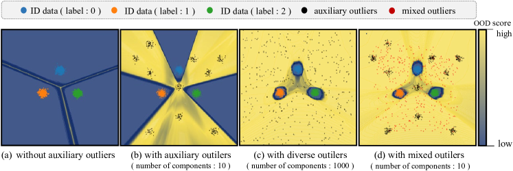
Figure 1: OOD score for different training strategies. The ID data $\mathcal{X}_{in}\subset\mathbb{R}^{2}$ is sampled from three distinct Gaussian distributions, each representing a different class. The auxiliary outliers are sampled from a Gaussian mixture model away from the ID data, where the number of mixture components indicates the number of classes contained in auxiliary outliers. (a) The model trained without auxiliary outliers fails to detect OOD. (b) Incorporating a less diverse set of auxiliary outliers (10 classes) during training enables partial OOD detection, but overfits auxiliary outliers. (c) OOD detection is improved with a more diverse set of auxiliary outliers (1000 classes). (d) diverseMix enriches the diversity of outliers (10 classes) through creating significantly distinct mixed outliers.

In this work, we theoretically investigate this crucial question from the perspective of generalization ability [3]. Specifically, we first conduct a theoretical analysis to demonstrate how the distribution shift between auxiliary outlier training set and test OOD data affects the generalization capability of OOD detector. Accordingly, a generalization bound is induced on the test-time OOD detection error of classifier, considering both empirical error and the error caused by the distribution shift between test OOD data and auxiliary outliers. Based on the theory, we deduce an intuitive conclusion that a more diverse set of auxiliary outliers can reduce the distribution shift error and effectively lower the upper bound of the OOD detection error. As shown in Figure 1(b)-(c), the model trained with a more diverse set of auxiliary outliers achieves better OOD detection. However, in practice, it is difficult and costly to collect sufficiently diverse outlier data. Therefore, a natural question arises - how to guarantee the effective utilization of a fixed set of auxiliary outliers?

Inspired from the theoretical principles, we propose a simple yet effective method called Diversity-induced Mixup (diverseMix) for OOD detection, which introduces and improves the mixup strategy to enhance the outlier diversity. Specifically, diverseMix employs semantic-level interpolation to generate mixed samples, creating new outliers that significantly deviate from their original counterparts. Given the risk that a random interpolation strategy (merely sampling from a predefined prior distribution) might produce mixed outliers that are unhelpful for the model (as the model can already detect them effectively), diverseMix dynamically adjusts its interpolation strategy based on original samples. This adjustment ensures that the generated outliers are novel and distinct from those previously encountered by the model, thereby enhancing diversity throughout the training process. As shown in Figure 1(b)-(d), diverseMix effectively boosts the diversity of auxiliary outliers, leading to improved OOD detection performance. The contributions of this paper are summarized as follows:

• We provide a theoretical analysis of the generalization error linked to methods trained with auxiliary outliers. By establishing an upper bound for expected error, we reveal the connection between auxiliary outlier diversity and the upper bound of OOD detection error. Our theoretical insights emphasize the importance of leveraging diverse auxiliary outliers to enhance the generalization capacity of the OOD detector.

• Constrained by the prohibitive cost of collecting outliers with sufficient diversity, we propose the Diversity-induced Mixup (diverseMix) for OOD detection, a simple yet effective strategy which is theoretically guaranteed to improve OOD detection performance.

• The proposed diverseMix achieves state-of-the-art OOD detection performance, outperforming existing methods on both standard and recent large-scale benchmarks. Remarkably, our method exhibits significant improvements over advanced methods, showing relative performance improvements of $24.4\%$ and $43.8\%$ (in terms of FPR95) on the CIFAR-10 and CIFAR-100 datasets, respectively.

2 Related Works

We provide a brief review of prior research relevant to our work followed by a comparison.

Auxiliary-Outlier-Free OOD Detection. One early work by [19] pioneered the field of OOD detection, introducing a baseline method based on maximum softmax probability. However, it has since been established, as noted by [36], that this approach is not quite suitable for OOD detection. To address this, various methods have been developed that operate in the logit space to enhance OOD detection. These include ODIN [25], energy score [46; 28; 45], ReAct [40], logit normalization [48], Mahalanobis distance [23], and KNN-based scoring [41]. However, post-hoc OOD detection methods that do not involve pre-training on a substantial dataset generally exhibit poorer performance compared to methods that leverage auxiliary datasets for model regularization  [13].

OOD Detection with Auxiliary Outliers. Recent advancements in OOD detection have focused on incorporating easily available auxiliary outliers into the model regularization process. Outlier exposure [20] encourage models to predict uniform distributions for outliers, and Energy-based learning [46] widens the energy gap between ID and OOD distribution. However, performance heavily depends on outlier quality. ATOM [6], POEM [34], and DOS [22] enhance performance by improving the sampling strategy for auxiliary outliers. DivOE [59] and DAL [47] improve outlier quality in a learnable manner, either in the sample space or feature space, respectively. Additionally, DOE implicitly enhances outlier informativeness through model perturbation. Incorporating outliers during training often achiveves superior performance, as shown in many other works [46; 39; 2; 48].

Comparison with Existing Methods. Several existing methods have explored the utilization of mixup in OOD detection. MixOE [56] and OpenMix [58] perform mixup between ID data and outliers, linearly representing the transition from ID to OOD and thus enhancing the model capturing the uncertainty from outliers. Meanwhile, MixOOD [51] employ mixup on ID data to generate outliers for training. Different from existing research which primarily focuses on refining mixup strategy or designing outlier regularization method, we place emphasis on the theoretical significance of auxiliary outlier diversity. Our approach advances this concept by enhancing outlier diversity via mixup based strategy, guaranteed by a robust theoretical framework. This focus on enhancing the diversity of auxiliary outliers distinguishes our research from prevailing studies in this area.

3 Theory: Diverse Auxiliary Outliers Boost OOD Detection

In this section, we lay the foundation for our analysis of OOD detection. We begin by introducing the key notations for OOD detection in Sec. 3.1. In Sec. 3.2, we establish a generalization bound which highlights the critical role for auxiliary outliers in influencing the generalization capacity of OOD detection methods. Finally, in Sec. 3.3, we demonstrate how a diverse set of auxiliary outliers effectively mitigate the distribution shift errors, consequently lowering the upper bound of error. For detailed proofs, please refer to Appendix A.

3.1 Preliminaries

We consider the multi-class classification task and each sample in the training set $\mathcal{D}_{id}=\{(x_{i},y_{i})\}^{N}_{i=1}$ is drawn i.i.d. from the joint distribution $\mathcal{P}_{\mathcal{X}_{id}\times\mathcal{Y}_{id}}$, where $\mathcal{X}_{id}$ denotes the input space of ID data, and $\mathcal{Y}_{id}=\{1,2,\ldots,K\}$ represents the label space. OOD detection can be formulated as a binary classification problem to learn a hypothesis $h$ from hypothesis space $\mathcal{H}\subset\{h:\mathcal{X}\rightarrow\{0,1\}\}$ such that $h$ outputs $1$ for any $x\in\mathcal{X}_{id}$ and $0$ for any $x\in\mathcal{X}_{ood}$, where $\mathcal{X}_{ood}=\mathcal{X}\setminus\mathcal{X}_{id}$ represent the input space of OOD data and $\mathcal{X}$ represents the entire input space in the open-world setting. To address the challenge posed by the unknown and arbitrariness of OOD distribution $\mathcal{P}_{\mathcal{X}_{ood}}$, we leverage an auxiliary dataset $\mathcal{D}_{aux}$ drawn from the distribution $\mathcal{P}_{\mathcal{X}_{aux}}$ to serve as partial OOD data, where $\mathcal{X}_{aux}\subset\mathcal{X}_{ood}$. Due to the diversity of real-world OOD data, auxiliary outliers cannot fully represent all OOD data, so $\mathcal{P}_{\mathcal{X}_{aux}}\neq\mathcal{P}_{\mathcal{X}_{ood}}$. We aim to train a model on data sampled from $\mathcal{P}_{\widetilde{\mathcal{X}}}=k_{train}\mathcal{P}_{\mathcal{X}_{id}}+(1-k_{train})\mathcal{P}_{\mathcal{X}_{aux}}$ to obtain a reliable hypothesis $h$ that can effectively generalize to the unknown test-time distribution $\mathcal{P}_{\mathcal{X}}=k_{test}\mathcal{P}_{\mathcal{X}_{id}}+(1-k_{test})\mathcal{P}_{\mathcal{X}_{ood}}$, where $k_{train}$ and $k_{test}$ determine the proportion of ID and OOD data used for training and testing, respectively. Note that $k_{test}$ is unknown due to unpredictable test data distribution.

3.2 Generalization Error Bound in OOD Detection

Basic Setting. We define an OOD label function which provides ground truth labels (OOD or ID) for inputs as $f:\mathcal{X}\rightarrow[0,1]$. The expectation that a hypothesis $h$ disagrees with $f$ with respect to a distribution $\mathcal{P}$ is defined as:

$$\epsilon_{\mathcal{P}}(h,f)=E_{x\sim\mathcal{P}}[|h(x)-f(x)|].$$ (1)

The set of ideal hypotheses on the training data distribution $P_{\widetilde{\mathcal{X}}}$ and test-time data distribution $P_{\mathcal{X}}$ is defined as:

$$\mathcal{H}^{*}_{aux}:h=\arg\min\limits_{h\in\mathcal{H}}\epsilon_{P_{\widetilde{\mathcal{X}}}}(h,f),\ \mathcal{H}^{*}_{ood}:h=\arg\min\limits_{h\in\mathcal{H}}\epsilon_{P_{\mathcal{X}}}(h,f),$$ (2)

and we define $h^{*}_{ood}$ and $h^{*}_{aux}$ as the element in $\mathcal{H}^{*}_{ood}$ and $\mathcal{H}^{*}_{aux}$, respectively, which can be denoted as $h^{*}_{ood}\in\mathcal{H}^{*}_{ood}$, $h^{*}_{aux}\in\mathcal{H}^{*}_{aux}$. Considering that $\mathcal{X}_{aux}\subset\mathcal{X}_{ood}$, it follows that $\mathcal{H}^{*}_{ood}\subseteq\mathcal{H}^{*}_{aux}$ , reflecting the reality that hypotheses perform well on real-world OOD data also perform well on auxiliary outliers, conditioning on that auxiliary outliers are a subset of real-world OOD data. The generalization error of an OOD detector $h$ is defined as:

$$\text{GError}(h)=\epsilon_{x\sim\mathcal{P}_{\mathcal{X}}}(h,f).$$ (3)

Now, we present our first main result regarding OOD detection (training with auxiliary outliers).

Theorem 1

(Generalization Bound of OOD Detector). We let $\mathcal{D}_{train}=\mathcal{D}_{id}\cup\mathcal{D}_{aux}$, consisting of $M$ samples. For any hypothesis $h\in\mathcal{H}$ and $0<\delta<1$, with a probability of at least $1-\delta$, the following inequality holds:

$$\begin{split}\text{GError}(h)\leq\underbrace{\hat{\epsilon}_{x\sim\mathcal{P}_{\widetilde{\mathcal{X}}}}(h,f)}_{\text{empirical error}}+\underbrace{\epsilon(h,h^{*}_{aux})}_{\text{reducible error}}+{\color[rgb]{0.82421875,0.33203125,0.33203125}\underbrace{\underset{h\in\mathcal{H}^{*}_{aux}}{\sup}\epsilon_{x\sim\mathcal{P}_{\mathcal{X}}}(h,h^{*}_{ood})}_{{\text{distribution shift error}}}}+\underbrace{\mathcal{R}_{m}(\mathcal{H})}_{\text{complexity}}+\sqrt{\frac{\ln(\frac{1}{\delta})}{2M}}+\beta,\end{split}$$ (4)

where $\hat{\epsilon}_{x\sim\mathcal{P}_{\widetilde{\mathcal{X}}}}(h,f)$ is the empirical error. We define $\epsilon(h,h^{*}_{aux})=\int|\phi_{\mathcal{X}}(x)-\phi_{\widetilde{\mathcal{X}}}(x)||h(x)-h^{*}_{aux}(x)|dx$ as the reducible error, where $\phi_{\mathcal{X}}$ and $\phi_{\widetilde{\mathcal{X}}}$ is the density function of $\mathcal{P}_{\mathcal{X}}$ and $\mathcal{P}_{\widetilde{\mathcal{X}}}$ respectively. $\underset{h\in\mathcal{H}^{*}_{aux}}{\sup}\epsilon_{x\sim\mathcal{P}_{\mathcal{X}}}(h,h^{*}_{ood})$ is the distribution shift error, $\mathcal{R}_{m}(\mathcal{H})$ represents the Rademacher complexity, and $\beta$ is some constant condition on the error related to ideal hypotheses.

Minimizing empirical risk optimizes the model $h$ to $h\in\mathcal{H}^{*}_{aux}$, leading to a reduction in the reducible error, which tends to zero. However, the inherent distribution shift error between auxiliary outliers and real-world OOD data remains constant and non-negligible. This limitation fundamentally restricts the generalization of OOD detection methods trained with auxiliary outliers. To address this limitation, we investigate the effect of outlier diversity on mitigating the distribution shift error.

3.3 Generalization with Auxiliary OOD Diversification

In this paper, the diversity refers to semantic diversity, where a formal definition is given as follows.

Definition 1

(Diversity of Outliers). We assume $\mathcal{X}_{aux}$ can be divided into distinct semantic groups: $\mathcal{X}_{aux}=\mathcal{X}^{y_{1}}\cup\mathcal{X}^{y_{2}}\cup\ldots\cup\mathcal{X}^{y_{m}}$, where each group $\mathcal{X}^{y_{i}}$ contains data points with label $y_{i}$. Considering a dataset $\mathcal{D}_{div}$ sampled from the distribution $\mathcal{P}_{\mathcal{X}_{div}}$, where $\mathcal{X}_{div}\subset\mathcal{X}_{ood}$ encompasses $\mathcal{X}_{aux}$ and an additional group $\mathcal{X}_{new}=\mathcal{X}^{y_{m+1}}\ldots\cup\mathcal{X}^{y_{n}}$ with different semantic compared to $\mathcal{X}_{aux}$, i.e., $\mathcal{X}_{div}=\mathcal{X}_{aux}\cup\mathcal{X}_{new}$, we define $\mathcal{D}_{div}$ is more diverse than $\mathcal{D}_{aux}$ in terms of the range of semantic classes covered.

Suppose we could use this diverse auxiliary outliers dataset for training, the ideal hypotheses achieved by training with $\mathcal{D}_{div}$ are denoted as:

$$\mathcal{H}^{*}_{div}:h=\arg\min\limits_{h\in\mathcal{H}}\epsilon_{x\sim\mathcal{P}_{\widetilde{\mathcal{X}}_{div}}}(h,f),$$ (5)

with $\mathcal{P}_{\widetilde{\mathcal{X}}_{div}}=k_{train}\mathcal{P}_{\mathcal{X}_{id}}+(1-k_{train})\mathcal{P}_{\mathcal{X}_{div}}$. Because $\mathcal{X}_{aux}\subset\mathcal{X}_{div}$ holds, the hypotheses performing well on $\mathcal{P}_{\mathcal{X}_{div}}$ also perform well on $\mathcal{P}_{\mathcal{X}_{aux}}$, giving rise to $\mathcal{H}^{*}_{div}\subset\mathcal{H}^{*}_{aux}$. Consequently, we have:

$$\underset{h\in\mathcal{H}^{*}_{div}}{sup}\epsilon_{x\sim\mathcal{P}_{\mathcal{X}}}(h,h^{*}_{ood})\leq\underset{h\in\mathcal{H}^{*}_{aux}}{sup}\epsilon_{x\sim\mathcal{P}_{\mathcal{X}}}(h,h^{*}_{ood}),$$ (6)

which indicates that training with a more diverse set of auxiliary outliers can reduce the distribution shift error. Furthermore, effective training leads to sufficient small empirical error and reducible error, and the intrinsic complexity of the model remains constant. Consequently, a more diverse set of auxiliary outliers results in a lower generalization error bound. This theorem is formalized as:

Theorem 2

(Diverse Outliers Enhance Generalization). Let $\mathcal{O}(\text{GError}(h))$ and $\mathcal{O}(\text{GError}(h_{div}))$ represent the upper bounds of the generalization error of detector training with vanilla auxiliary outliers $\mathcal{D}_{aux}$ and diverse auxiliary outliers $\mathcal{D}_{div}$, respectively. For any hypothesis $h$ and $h_{div}$ in $\mathcal{H}$, and $0<\delta<1$, with a probability of at least $1-\delta$, the following inequality holds

$$\mathcal{O}(\text{GError}(h_{div}))\leq\mathcal{O}(\text{GError}(h)).$$ (7)

Remark. Theorem 2 highlights that the diversity of the outlier set is a critical factor in reducing the upper bound of generalization error. However, despite the fundamental improvement in model generalization achieved by increasing the diversity of auxiliary outliers, collecting a more diverse set of auxiliary outliers is expensive, and the auxiliary outliers we can use are limited in practical scenarios, which hinders the application of outlier exposure based methods for OOD detection. This raises an intuitive question: can we enhance the diversity of a fixed outlier set for better utilization?

4 Method: Diversity-induced Mixup (diverseMix)

In this section, we show how diverseMix addresses the challenge of effective training when the outlier diversity is limited. We begin with a theoretical analysis demonstrating the effectiveness of mixup in enhancing outlier diversity to improve OOD detection performance, providing a reliable guarantee for our mixup-based method. Then, we introduce a simple yet effective framework implementing our method diverseMix to enhance OOD detection performance.

4.1 Theoretical Insights: Semantic Interpolation Guarantees Enhanced Diversity of Outliers

Mixup [55] is a widely used machine learning technique to augment training data by creating synthetic samples, which has been extensively utilized in various studies[17; 7; 52]. It involves generating virtual training samples (referred to as mixed samples) through linear interpolations between data points and corresponding labels, given by:

$$\hat{x}=\lambda x_{i}+(1-\lambda)x_{j},\quad\hat{y}=\lambda y_{i}+(1-\lambda)y_{j},$$ (8)

where $(x_{i},y_{i})$ and $(x_{j},y_{j})$ are two samples drawn randomly from the empirical training distribution, and $\lambda\in[0,1]$ is usually sampled from a Beta distribution with parameter $\alpha$ denoted as $Beta(\alpha,\alpha)$. This technique assumes a linear relationship between semantics (labels) and features (in data), allowing us to create new mixed samples that deviate significantly from the semantics of the original ones by combining features from samples with distinct semantics. These new mixed samples are situated outside of the original data manifold [16]. We summarize this assumption as follows:

Assumption 1

(Semantic Change under Mixup). Let $x_{i}$ and $x_{j}$ be any two data points from input spaces $\mathcal{X}^{y_{i}}$ and $\mathcal{X}^{y_{j}}$, respectively, where $y_{i}$ and $y_{j}$ are corresponding semantic labels and $y_{i}\neq y_{j}$. If $\zeta<\lambda<1-\zeta$, then there exists a positive value $\zeta$ such that the mixed data point $\hat{x}=\lambda x_{i}+(1-\lambda)x_{j}$ does not belong to either $\mathcal{X}^{y_{i}}$ or $\mathcal{X}^{y_{j}}$.

This assumption suggests that we can enhance the diversity of outliers by generating new outliers with distinct semantics using mixup. Specifically, applying mixup to outliers in $\mathcal{X}_{aux}$ results in some generated mixed outliers having different semantics, suggesting that they belong to novel (unknown or unnamed) semantic classes outside of $\mathcal{X}_{aux}$. Consequently, these mixed outliers can be considered as samples from a broader region within the input space. As per Definition 1, the mixed outliers exhibit greater diversity than the original outliers. This lemma is formally presented as follows:

Lemma 1

(Diversity Enhancement with Mixup). For a group of mixup transforms $\mathcal{G}$ acting on the input space $\mathcal{X}_{aux}$ to generate an augmented input space $\mathcal{G}\mathcal{X}_{aux}$, defined as $\mathcal{G}\mathcal{X}_{aux}=\{\hat{x}|\hat{x}=\lambda x_{1}+(1-\lambda)x_{2};x_{1},x_{2}\in\mathcal{X}_{aux},\lambda\in[0,1]\}$, the following relation holds:

$$\mathcal{X}_{aux}\subset\mathcal{G}\mathcal{X}_{aux}.$$ (9)

Lemma 1 establishes that mixed outliers $\mathcal{D}_{mix}$ exhibits greater diversity compared to $\mathcal{D}_{aux}$, where $\mathcal{D}_{mix}$ is drawn from distribution $\mathcal{P}_{\mathcal{G}\mathcal{X}_{aux}}$. Consequently, according to Theorem 2, mixup outliers contribute to a reduction in generalization error. We can formalize this relationship as follows, and the detailed proofs can be found in Appendix A.

Theorem 3

(Mixed Outlier Enhances Generalization). Let $\mathcal{O}(\text{GError}(h))$ and $\mathcal{O}(\text{GError}(h_{mix}))$ represent the upper bounds of the generalization error of detector training with vanilla auxiliary outliers $\mathcal{D}_{aux}$ and mixed auxiliary outliers $\mathcal{D}_{mix}$, respectively. For any hypothesis $h$ and $h_{mix}$ in $\mathcal{H}$, and $0<\delta<1$, with a probability of at least $1-\delta$, we have

$$\mathcal{O}(\text{GError}(h_{mix}))\leq\mathcal{O}(\text{GError}(h)).$$ (10)

Theorem 3 demonstrates that mixup enhances auxiliary outlier diversity, reducing the upper bound of generalization error in OOD detection, which provides a reliable guarantee of mixup’s effectiveness in improving OOD detection. However, the vanilla mixup lacks flexibility, which may generate outliers that are not necessarily beneficial to the model. Next, we will provide an implementation of our method which dynamically adjusts the interpolation strategy in a data-adaptive manner.

4.2 Implementation

Considering a classifier network $\theta$ and $F(x,\theta)$ denotes the logit outputs for input $x$, our goal is to use the scoring function $S(x,\theta)$ to develop an OOD detector:

$$G(x)=\text{ID}\cdot\mathbf{1}\{S(x,\theta)\geq\gamma\}+\text{OOD}\cdot\mathbf{1}\{S(x,\theta)<\gamma\},$$ (11)

where $\mathbf{1}\{\cdot\}$ is the indicator function, $\gamma$ is the threshold, typically chosen to ensure that a significant proportion (e.g., 95%) of ID data is accurately identified. The training objective is given by:

$$\begin{aligned} \arg\min\limits_{\theta}\ \mathbb{E}_{(x,y)\sim\mathcal{D}_{id}}[\mathcal{L}_{\text{CE}}(F(x,\theta),y)]+\omega\cdot\mathcal{L}_{\text{aux}},\end{aligned}$$ (12)

where $\mathcal{L}_{\text{CE}}(\cdot)$ is the cross entropy loss, $\mathcal{L}_{\text{aux}}$ serves as a regularization term enabling model to learn from auxiliary outliers with low-confidence predictions, and $\omega$ controls the strength of regularization.

Our previous analysis showed that semantic interpolation can increase the diversity of outliers, thereby enhancing the model’s OOD detection performance. However, the interpolation weights in vanilla mixup is randomly sampled from a preset prior distribution (e.g. beta distribution), which may result in generating mixed outliers that are not necessarily beneficial to the model. To efficiently increase the diversity of auxiliary outliers, we dynamically adjust the mixup strategy based on the original outliers, thereby generating novel mixed outliers which are more likely to be unfamiliar to the model.

During each training epoch, outliers are regularized, prompting the model $\theta$ to assign lower scores to previously encountered outliers. Consequently, outliers that achieve higher scores $S(x,\theta)$ are more likely to be novel or previously unseen outliers. We expect the generated outliers to be located in the vicinal space of the novel outliers that have not yet been encountered by the model. To achieve this, we adjust the prior distribution based on scores. Specifically, for outlier samples $x_{i}$ and $x_{j}$ randomly drawn from the empirical auxiliary outlier distribution, the mixed outliers are formulated as follows:

$$\hat{x}=\lambda x_{i}+(1-\lambda)x_{j},\ \lambda\sim\text{Beta}(\hat{s}_{i}\alpha,\hat{s}_{j}\alpha),$$ (13)

where $\hat{s}_{i}$,$\hat{s}_{j}$ adjusts the original Beta distribution according to $x_{i}$ and $x_{j}$, which is defined as follows:

$$\hat{s}_{i}=\frac{\exp(S(x_{i},\theta)/T)}{\sum_{k\in\{i,j\}}\exp(S(x_{k},\theta)/T)},$$ (14)

with $T$ representing the temperature parameter. This adaptive strategy assigns higher weights to the outliers that contain more information unknown to the current model, ensuring the generation of novel outliers, thereby increasing diversity throughout the training process. After constructing the mixed auxiliary outliers, they are used for the training objective (12). The whole pseudo code of the proposed method is shown in Alg. 1.

Input: ID dataset $\mathcal{D}_{\text{id}}$, outlier dataset $\mathcal{D}_{\text{aux}}$, batch size $N$, distribution parameter $\alpha$, temperature $T$.

Output: model parameters $\theta$.

for each iteration do

       for each mini-batch do

            

            Sample $N$ ID data from $\mathcal{D}_{\text{id}}$ as $\mathcal{B}_{\text{id}}$ and $N$ outliers from $\mathcal{D}_{\text{aux}}$ as $\mathcal{B}_{\text{aux}}$, respectively.

            Evaluate the auxiliary outliers $\mathcal{B}_{\text{aux}}$ using the current model $\theta$ to obtain the scores $\mathcal{S}$.

            Randomly shuffle $\mathcal{B}_{\text{aux}}$ and the corresponding scores $\mathcal{S}$ to generate $\mathcal{B}_{\text{aux}}^{\prime}$ and $\mathcal{S}^{\prime}$.

            Generate prior adjustment strategies based on scores $\mathcal{S}$ and $\mathcal{S}^{\prime}$ according to Eq. 14.

            Sample the interpolation weight from the adjusted prior distribution and generate mixed outliers $\mathcal{D}_{mix}$ according to Eq. 13.

            Train the model $\theta$ using the objective function defined in Eq. 12.

      end for

end for

Algorithm 1 diverseMix for OOD Detection

Compatibility with different OOD regularization method. DiverseMix is a general method that is suitable for a series of OOD regularization methods. One representative method is the energy-based method [46], which employs the following OOD regularization loss:

$$\mathcal{L}_{aux}=\mathbb{E}_{(x,y)\sim\mathcal{D}_{id}}[(\max(0,m_{in}-S(x;\theta))^{2}]+\mathbb{E}_{x\sim\mathcal{D}_{aux}}[(\max(0,S(x;\theta)-m_{out}))^{2}],$$ (15)

where $m_{in}$ and $m_{out}$ are margin hyperparameters, and $S(x;\theta)=\log\sum^{K}_{i=1}\exp(F_{i}(x,\theta))$ is the corresponding scoring function. More details for regularization methods are provided in Appendix B.3.

5 Experiments

In this section, we outline our experimental setup and conduct experiments on common OOD detection benchmarks to answer the following questions: Q1. Effectiveness (I): Does our method outperform its counterparts in OOD detection? Q2. Effectiveness (II): Does our method retain its superior performance across various settings including large-scale benchmark? Q3. Practicability (I): Does our method demonstrate effectiveness across different OOD regularization methods? Q4. Practicability (II): Does our method demonstrate effectiveness in low-quality of auxiliary outliers dataset? Q5. Ablation study: (I) Does diverseMix truly offer a distinct advantage over other data augmentation methods? (II) What is the key factor contributing to performance improvement in our method? Q6. Reliability: Do the experimental results provide strong support for established theory?

5.1 Experimental Setup

We briefly present the experimental setup here, including the experimental datasets and evaluation metrics. Further experimental details can be found in Appendix B.

Datasets. $\circ$ ID datasets. Following the commonly used benchmark in OOD detection literature, we use CIFAR-10, CIFAR-100 and ImageNet-200 as ID datasets. $\circ$ Auxiliary outlier datasets. For CIFAR experiments, the downsampled version of ImageNet (ImageNet-RC) is employed as auxiliary outliers. For ImageNet-200 experiments, the remaining 800 categories from ImageNet-1k (ImageNet-800) serve as auxiliary outliers. $\circ$ OOD test sets. For CIFAR benchmark, we use diverse datasets including SVHN [37], Textures [8], Places365 [57], LSUN-crop, LSUN-resize [53], and iSUN [49]. For ImageNet benchmark, We use datasets such as SSB-hard [43], NINCO [5], iNaturalist [42], Textures [8] and OpenImage-O [44].

Evaluation metrics. Following common practice, we report: (1) OOD false positive rate at 95% true positive rate for ID samples (FPR95) [26], (2) the area under the receiver operating characteristic curve (AUROC) [10], (3) the area under the precision-recall curve (AUPR) [31]. We also provide ID classification accuracy (ID-ACC).

5.2 Experimental Results and Discussion

DiverseMix achieves superior performance on the common benchmark (Q1). Our method outperforms existing competitive methods, establishing state-of-the-art performance both on CIFAR-10 and CIFAR-100 datasets. Table 1 provides a comprehensive comparison with methods grouped into: (1) ID-only training: MSP [19], ODIN [25], Mahalanobis [23], Energy [46]; (2) Utilizing auxiliary outliers: OE [20], SOFL [35], CCU [32], Energy with outliers [46], NTOM [6], POEM [34], MixOE [56], DivOE [59]. Methods that utilizing auxiliary outliers generally achieve significantly better empirical performance on OOD detection. This implies that leveraging auxiliary outliers is essential for enhancing OOD detection performance. Our method diverseMix significantly outperforms the top baseline, reducing the FPR95 by 0.62% and 6.63% on CIFAR-10 and CIFAR-100, respectively. These reductions correspond to relative error reductions of 24.4% and 43.8%. These notable improvements can be attributed to the enhanced diversity in auxiliary outliers offered by diverseMix, which lowers the generalization error bound and significantly improves the OOD detection performance.

Table 1: Main results. Comparison with competitive OOD detection methods trained with the same DenseNet backbone. The performance metrics are averaged (%) over six OOD test datasets from Section 5.1. The best results are in bold. diverseMix not only demonstrates state-of-the-art OOD detection performance on the CIFAR benchmark but also maintains high accuracy in ID classification. More details are provided in the Appendix B.

Method	CIFAR-10				CIFAR-100				w./w.o. $\mathcal{D}_{aux}$
	FPR95 ($\downarrow$)	AUROC ($\uparrow$)	AUPR ($\uparrow$)	ID-ACC	FPR95 ($\downarrow$)	AUROC ($\uparrow$)	AUPR ($\uparrow$)	ID-ACC
MSP	58.98	90.63	93.18	94.39	80.30	73.13	76.97	74.05	$\times$
ODIN	26.55	94.25	95.34	94.39	56.31	84.89	85.88	74.05	$\times$
Mahalanobis	29.47	89.96	89.70	94.39	47.89	85.71	87.15	74.05	$\times$
Energy	28.53	94.39	95.56	94.39	65.87	81.50	84.07	74.05	$\times$
SSD+	7.22	98.48	98.59	NA	38.32	88.91	89.77	NA	$\times$
OE	9.66	98.34	98.55	94.12	19.54	94.93	95.26	74.25	$\checkmark$
SOFL	5.41	98.98	99.10	93.68	19.32	96.32	96.99	73.93	$\checkmark$
CCU	8.78	98.41	98.69	93.97	19.27	95.02	95.41	74.49	$\checkmark$
Energy (w. $\mathcal{D}_{aux}$)	4.62	98.93	99.12	92.92	19.25	96.68	97.44	72.39	$\checkmark$
NTOM	4.00	99.09	98.61	94.26	18.77	96.69	96.49	74.52	$\checkmark$
POEM	2.54	99.40	99.50	93.49	15.14	97.79	98.31	73.41	$\checkmark$
MixOE	14.54	97.16	97.41	94.48	27.71	92.93	93.81	75.15	$\checkmark$
DivOE	11.41	97.76	98.18	93.74	18.91	95.00	95.26	74.08	$\checkmark$
DiverseMix (ours)	1.92	99.42	99.51	94.16	8.51	98.24	98.46	74.60	$\checkmark$

Table 2: Main results on large-scale ImageNet benchmark. Comparison with competitive OOD detection methods trained with the same ResNet backbone. For better presentation, the best and second-best results are in bold and underline respectively. Consistent with CIFAR experiment results, diverseMix demonstrates strong OOD detection capabilities for both near-OOD and far-OOD test sets, achieving state-of-the-art OOD detection performance. Details are provided in the Appendix B.

Method	Near-OOD			Far-OOD			Average			ID-ACC
	FPR ($\downarrow$)	AUROC ($\uparrow$)	AUPR ($\uparrow$)	FPR ($\downarrow$)	AUROC ($\uparrow$)	AUPR ($\uparrow$)	FPR ($\downarrow$)	AUROC ($\uparrow$)	AUPR ($\uparrow$)
MSP	70.35	82.75	88.58	54.51	88.81	91.86	60.85	86.39	90.54	85.81
Energy	70.35	81.88	88.56	53.87	89.30	91.59	60.46	86.33	90.38	85.81
Max Logits	69.45	82.25	88.69	52.49	89.60	92.13	59.28	86.66	90.75	85.81
ODIN	69.06	82.20	88.75	50.90	89.90	92.50	58.16	86.82	91.00	85.81
OE	59.12	86.86	92.69	54.95	90.51	91.20	56.61	89.05	91.79	85.52
Energy (w. $D_{aux}$)	60.67	85.95	91.75	58.07	89.73	89.67	59.11	88.22	90.50	84.94
DPN	63.39	84.94	91.46	61.31	89.85	90.16	62.14	87.89	90.68	85.27
MixOE	68.43	83.42	88.74	50.51	90.62	92.31	57.68	87.38	90.89	86.35
DiverseMix (ours)	59.81	86.36	91.76	48.58	91.35	92.38	53.07	89.36	92.13	85.95

DiverseMix is effective on the large-scale benchmark (Q2). Recent studies  [50] have suggested that methods leveraging outlier data tend to underperform in more demanding, large-scale OOD detection tasks. To evaluate the effectiveness of our method, we conduct experiments on the ImageNet benchmark. Following[50], We categorize the OOD test set into two distinct groups: near-OOD and far-OOD. For each group, we report the average performance metrics. Furthermore, we also present the overall average performance on the OOD test sets. Table 2 illustrates that methods requiring outliers during training tend to excel in near OOD detection but fall short in far-OOD detection, sometimes even performing worse than methods that do not require outliers during training. Although MixOE improves far-OOD detection performance to some extent, it fails to fully leverage auxiliary outliers to enhance near-OOD detection. In contrast, our method not only maintains strong performance in near-OOD detection but also significantly improves performance in far-OOD scenarios. We speculate that the virtual auxiliary outlier data generated by diverseMix may be more representative of far-OOD data. While most OOD detection methods face difficulties in achieving satisfactory performance across both near-OOD and far-OOD, our method excels in detecting both types of OOD, significantly surpassing other methods in the average OOD detection performance.

DiverseMix is a general method that achieves good performance across different OOD regularization methods (Q3). To investigate the generality of diverseMix across different OOD regularization methods, we replace the original energy loss with the K+1 loss and the OE loss. The experimental results presented in Figure 2 reveal that diverseMix achieves consistent effectiveness regardless of the OOD regularization method employed. These findings not only suggest the versatility of our method but also provide substantial empirical evidence supporting our theoretical framework.

DiverseMix remains effective even when the auxiliary outlier data is of low quality (Q4). In Figure 2, the quality of auxiliary outliers used for training is decreased by gradually decreasing their quantity or their diversity. Our method diverseMix consistently outperforms previous methods by enhancing the diversity of auxiliary outliers across different dataset sizes and diversity levels. This suggests that diverseMix remains effective even when the auxiliary outliers are of low quality.

Sample adaptive semantic interpolation contributing to unique advantages of diverseMix (Q5). We compared diverseMix with other data augmentation methods. As shown in Table 3(a), diverseMix demonstrates superior performance for OOD detection over other data augmentation methods that preserve the semantics of outliers. Additionally, the ablation study in Table 3(b) compares diverseMix with different mixup strategies. DiverseMix outperforms both vanilla mixup and cutmix by adaptively adjusting its interpolation strategy based on the given outliers, thereby efficiently generating novel mixed outlier samples to enhance diversity. The advantages of diverseMix lie in 1) enhancing the diversity of outliers at the semantic level, and 2) efficiently boosting diversity by adaptively adjusting its strategy for the given outlier samples. For detailed comparisons, please see Appendix B.6.

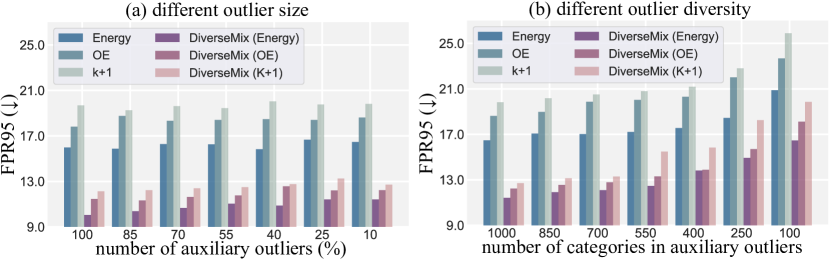
Figure 2: Comparison of OOD detection performance on CIFAR-100 with decreased quality of auxiliary outlier datasets (a) With constant diversity of auxiliary outliers (1000 categories), the dataset size is decreased. The x-axis represents the percentage of the original outlier dataset’s size used for training. (b) With fixed dataset size (10% of auxiliary outliers), the diversity of outliers is decreased, with the x-axis displaying the number of categories. See Appendix B.4 for more details.

Table 3: Ablation study. Performance are averaged (%) over six OOD test datasets from Section  5.1. The best results are in bold. More details about the comparison methods are provided in Appendix B

(a) different data augmentation method. CIFAR-10 CIFAR-100 FPR ($\downarrow$) AUROC ($\uparrow$) FPR ($\downarrow$) AUROC ($\uparrow$) Gaussian noise 6.69 98.64 19.94 95.69 Cutout 7.20 98.57 19.12 96.64 Color jitter 8.83 98.45 24.36 95.01 DiverseMix (ours) 1.92 99.42 8.51 98.24

(b) different semantic interpolation strategy. CIFAR-10 CIFAR-100 FPR ($\downarrow$) AUROC ($\uparrow$) FPR ($\downarrow$) AUROC ($\uparrow$) Vanilla 5.43 98.80 16.30 96.87 Mixup 4.00 99.02 12.56 97.42 Cutmix 5.76 98.79 15.95 97.06 DiverseMix (ours) 1.92 99.42 8.51 98.24

Our theory effectively demonstrates that the diversity of auxiliary outliers is a key factor to ensure OOD detection performance (Q6). In Figure 2, when maintaining the diversity relatively constant and changing the quantity of data, the performance of different methods remains relatively stable. However, when the number of outliers is fixed and the diversity of the outliers dataset is reduced, there is a significant decrease in performance across all methods. This suggests that diversity is a key quality factor for the auxiliary outliers, providing substantial empirical support for our theory.

DiverseMix has the potential for application across a wide range of task domains. Our theory is not rely on any assumptions specific to the task domain. Given the successful implementation of mixup across different fields [15; 54], diverseMix also has the potential for application in multiple task domains beyond just computer vision tasks. We have investigated the application of diverseMix in the NLP domain through experiments. For additional details, please see Appendix  C.2.

6 Conclusions and Future Work

In this study, we demonstrate that the performance of OOD detection methods is hindered by the distribution shift between unknown test OOD data and auxiliary outliers. Through rigorous theoretical analysis, we demonstrate that enhancing the diversity of auxiliary outliers can effectively mitigate this problem. Constrained by limited access to auxiliary outliers and the high cost of data collection, we introduce diverseMix, an effective method that enhances the diversity of auxiliary outliers and significantly improves model performance. The effectiveness of diverseMix is supported by both theoretical analysis and empirical evidence. Furthermore, our theory enables future research to design new OOD detection method. We hope that our research can bring more attention to the diversity in OOD detection.

7 Acknowledgements

This work was supported by the National Natural Science Foundation of China (Grant No.62376193), the National Science Fund for Distinguished Young Scholars (Grant No.61925602) and the H. Fu’s Agency for Science, Technology and Research (A*STAR) Central Research Fund (“Robust and Trustworthy AI system for Multi-modality Healthcare”). The authors also appreciate the suggestions from NeurIPS anonymous peer reviewers.

[appendices]

Contents

[appendices]0

Appendix A Theoretical Analysis

In this section, we provide detailed proofs of our theories and the proposed method, including the proof of $\mathcal{H}^{*}_{ood}\subseteq\mathcal{H}^{*}_{aux}$, the establishment of the generalization error bound for OOD detection (Theorem 1), a more diverse set of auxiliary outliers leads to a reduced generalization error (Theorem 2), and the proof of diversity enhancement with mixup (Lemma 1).

A.1 Proof of $\mathcal{H}^{*}_{ood}\subseteq\mathcal{H}^{*}_{aux}$

In this section, we demonstrate that if $\mathcal{H}$ consist of fully-connected ReLU network with width $d_{m}\leq n+4$, where $n$ is the input dimension, and given that that $\mathcal{X}_{aux}\subset\mathcal{X}_{ood}$, it follows that $\mathcal{H}^{*}_{ood}\subseteq\mathcal{H}^{*}_{aux}$, This reflects the reality that hypotheses perform well on real-world OOD data also perform well on auxiliary outliers, conditioning on that auxiliary outliers are a subset of real-world OOD data.

Proof. We first express the expected error of hypotheses $h$ on the training data distribution $\mathcal{P}_{\widetilde{\mathcal{X}}}$ and the unknown test-time data distribution $\mathcal{P}_{\mathcal{X}}$ as follows:

$$\begin{cases}\epsilon_{\mathcal{P}_{\widetilde{\mathcal{X}}}}(h,f)=\int_{\widetilde{\mathcal{X}}}|h(x)-f(x)|dx=\int_{\mathcal{X}_{aux}}|h(x)-f(x)|dx+\int_{\mathcal{X}_{id}}|h(x)-f(x)|dx=\epsilon_{1},\\ \int_{\mathcal{X}_{ood}\setminus\mathcal{X}_{aux}}|h(x)-f(x)|dx=\epsilon_{2},\\ \epsilon_{\mathcal{P}_{\mathcal{X}}}(h,f)=\int_{\mathcal{X}}|h(x)-f(x)|dx=\int_{\mathcal{X}_{id}}|h(x)-f(x)|dx+\int_{\mathcal{X}_{ood}}|h(x)-f(x)|dx\\ =\int_{\mathcal{X}_{id}}|h(x)-f(x)|dx+\int_{\mathcal{X}_{aux}}|h(x)-f(x)|dx+\int_{\mathcal{X}_{ood}\setminus\mathcal{X}_{aux}}|h(x)-f(x)|dx=\epsilon_{1}+\epsilon_{2}.\end{cases}$$

From the above expressions, we obtain:

$$\begin{cases}\mathcal{H}^{*}_{aux}=\{h:\arg\min\limits_{h}\epsilon_{1}\},\\ \mathcal{H}^{*}_{other}=\{h:\arg\min\limits_{h}\epsilon_{2}\},\\ \mathcal{H}^{*}_{ood}=\{h:\arg\min\limits_{h}(\epsilon_{1}+\epsilon_{2})\}.\end{cases}$$

Let $f^{\prime}$ be a function that minimizes both $\epsilon_{1}$ and $\epsilon_{2}$, considering that $\int_{\mathcal{X}}|f^{\prime}(x)|dx<\infty$, which implies that $f^{\prime}$ is Lebesgue-integrable on $\mathcal{X}$. The $\mathcal{H}$ represent the fully-connected ReLU networks with width $d_{m}\leq n+4$, where $n$ is the input dimension. According to the Universal Approximation Theorem for Width-Bounded ReLU Networks [30], for any $\epsilon>0$, there exists a $h\in\mathcal{H}$ such that: $\int_{\mathcal{X}}|h(x)-f^{\prime}(x)|dx<\epsilon$. Consequently, there exists a hypothesis $h\in\mathcal{H}$ that simultaneously minimizes both $\epsilon_{1}$ and $\epsilon_{2}$. leading to the condition $\mathcal{H}^{*}_{aux}\cap\mathcal{H}^{*}_{other}\neq\emptyset$. In this case, we have $\min\limits_{h}(\epsilon_{1}+\epsilon_{2})=\min\limits_{h}\epsilon_{1}+\min\limits_{h}\epsilon_{2}$. We denote $\mathcal{H}^{*}_{ood}=\mathcal{H}^{*}_{aux}\cap\mathcal{H}^{*}_{other}$, thus establishing that $\mathcal{H}^{*}_{ood}\subset\mathcal{H}^{*}_{aux}$.

A.2 Proof of Theorem 1

In this section, we analyze the generalization error of the OOD detector training with auxiliary outliers. First, we recall the setting from Sec. 3.1, our goal is to train a detector with auxiliary outliers that can perform well on real-world OOD data. In other words, we aim to train a model on data sampled from $\mathcal{P}_{\widetilde{\mathcal{X}}}=k_{train}\mathcal{P}_{\mathcal{X}_{id}}+(1-k_{train})\mathcal{P}_{\mathcal{X}_{aux}}$ to obtain a reliable hypothesis $h$ that can effectively generalize to the unknown test-time distribution $\mathcal{P}_{\mathcal{X}}=k_{test}\mathcal{P}_{\mathcal{X}_{id}}+(1-k_{test})\mathcal{P}_{\mathcal{X}_{ood}}$.

Next, we develop bounds on the OOD detection performance of a detector training with auxiliary outliers, which can be formulated as follow:

(Generalization Bound of OOD Detector). Let $\mathcal{D}_{train}=\mathcal{D}_{id}\cup\mathcal{D}_{aux}$, consisting of $M$ samples. For any hypothesis $h\in\mathcal{H}$ and $0<\delta<1$, with a probability of at least $1-\delta$, the following inequality holds:

$$\text{GError}(h)\leq\underbrace{\hat{\epsilon}_{x\sim\mathcal{P}_{\widetilde{\mathcal{X}}}}(h,f)}_{\text{empirical error}}+\underbrace{\epsilon(h,h^{*}_{aux})}_{\text{reducible error}}+{\color[rgb]{0.82421875,0.33203125,0.33203125}\underbrace{\underset{h\in\mathcal{H}^{*}_{aux}}{\sup}\epsilon_{x\sim\mathcal{P}_{\mathcal{X}}}(h,h^{*}_{ood})}_{\text{distribution shift error}}}+\underbrace{\mathcal{R}_{m}(\mathcal{H})}_{\text{complexity}}+\sqrt{\frac{\ln(\frac{1}{\delta})}{2M}}+\beta,$$ (16)

where $\hat{\epsilon}_{x\sim\mathcal{P}_{\widetilde{\mathcal{X}}}}(h,f)$ is the empirical error. We define $\epsilon(h,h^{*}_{aux})=\int|\phi_{\mathcal{X}}(x)-\phi_{\widetilde{\mathcal{X}}}(x)||h(x)-h^{*}_{aux}(x)|dx$ is the reducible error, $\phi_{\mathcal{X}}$ and $\phi_{\widetilde{\mathcal{X}}}$ is the density function of $\mathcal{P}_{\mathcal{X}}$ and $\mathcal{P}_{\widetilde{\mathcal{X}}}$ respectively. $\underset{h\in\mathcal{H}^{*}_{aux}}{\sup}\epsilon_{x\sim\mathcal{P}_{\mathcal{X}}}(h,h^{*}_{ood})$ is the distribution shift color, $\mathcal{R}_{m}(\mathcal{H})$ represents the Rademacher complexity, $\beta$ is the error related to ideal hypotheses. The roadmap of our analysis is as follows:

Roadmap. We first show how to bound the OOD detection error in terms of the generalization error on $\mathcal{P}_{\widetilde{\mathcal{X}}}$ and the maximum distribution shift error as well as the reducible error which can be reduced to a small value as the model is optimized. Then, we study the generalization bound from the perspective of Rademacher complexity. We use complexity-based learning theory to quantify the generalization error on $\mathcal{P}_{\widetilde{\mathcal{X}}}$. In the end, we bound the OOD detection generalization error in terms of the empirical error on the training data, the reducible error, the maximum distribution shift error, and the complexity. We also provide detailed proof steps as follows:

Proof. This proof relies on the triangle inequality for classification error [4, 9], which implies that for any labeling functions $f_{1}$, $f_{2}$, and $f_{3}$, we have $\epsilon(f_{1},f_{2})\leq\epsilon(f_{1},f_{3})+\epsilon(f_{2},f_{3})$.

$$GError(h)=\epsilon_{x\sim\mathcal{P}_{\mathcal{X}}}(h,f)$$

$$\leq\epsilon_{x\sim\mathcal{P}_{\mathcal{X}}}(h,h^{*}_{ood})+\epsilon_{x\sim\mathcal{P}_{\mathcal{X}}}(h^{*}_{ood},f)$$

$$=\epsilon_{x\sim\mathcal{P}_{\mathcal{X}}}(h,h^{*}_{ood})+\epsilon_{x\sim\mathcal{P}_{\mathcal{X}}}(h^{*}_{ood},f)+\epsilon_{x\sim\mathcal{P}_{\widetilde{\mathcal{X}}}}(h,h^{*}_{ood})-\epsilon_{x\sim\mathcal{P}_{\widetilde{\mathcal{X}}}}(h,h^{*}_{ood})$$

$$=\epsilon_{x\sim\mathcal{P}_{\widetilde{\mathcal{X}}}}(h,h^{*}_{ood})+\epsilon_{x\sim\mathcal{P}_{\mathcal{X}}}(h^{*}_{ood},f)+\epsilon_{x\sim\mathcal{P}_{\mathcal{X}}}(h,h^{*}_{ood})-\epsilon_{x\sim\mathcal{P}_{\widetilde{\mathcal{X}}}}(h,h^{*}_{ood})$$

$$\leq\epsilon_{x\sim\mathcal{P}_{\widetilde{\mathcal{X}}}}(h,f)+\epsilon_{x\sim\mathcal{P}_{\widetilde{\mathcal{X}}}}(h^{*}_{ood},f)+\epsilon_{x\sim\mathcal{P}_{\mathcal{X}}}(h^{*}_{ood},f)+\epsilon_{x\sim\mathcal{P}_{\mathcal{X}}}(h,h^{*}_{ood})-\epsilon_{x\sim\mathcal{P}_{\widetilde{\mathcal{X}}}}(h,h^{*}_{ood})$$

Let $\phi_{\mathcal{X}}$ and $\phi_{\widetilde{\mathcal{X}}}$ be the density functions of $\mathcal{P}_{\mathcal{X}}$ and $\mathcal{P}_{\widetilde{\mathcal{X}}}$, respectively.

$$\begin{split}GError(h)\leq\epsilon_{x\sim\mathcal{P}_{\widetilde{\mathcal{X}}}}(h,f)+\epsilon_{x\sim\mathcal{P}_{\widetilde{\mathcal{X}}}}(h^{*}_{ood},f)+\epsilon_{x\sim\mathcal{P}_{\mathcal{X}}}(h^{*}_{ood},f)\\ +\int\phi_{\mathcal{X}}(x)|h(x)-h^{*}_{ood}(x)|\,dx-\int\phi_{\widetilde{\mathcal{X}}}(x)|h(x)-h^{*}_{ood}(x)|\,dx\end{split}$$

$$\leq\epsilon_{x\sim\mathcal{P}_{\widetilde{\mathcal{X}}}}(h,f)+\epsilon_{x\sim\mathcal{P}_{\widetilde{\mathcal{X}}}}(h^{*}_{ood},f)+\epsilon_{x\sim\mathcal{P}_{\mathcal{X}}}(h^{*}_{ood},f)+\int|\phi_{\mathcal{X}}(x)-\phi_{\widetilde{\mathcal{X}}}(x)|\left|h(x)-h^{*}_{ood}(x)\right|\,dx$$

$$\begin{split}\leq\epsilon_{x\sim\mathcal{P}_{\widetilde{\mathcal{X}}}}(h,f)+\epsilon_{x\sim\mathcal{P}_{\widetilde{\mathcal{X}}}}(h^{*}_{ood},f)+\epsilon_{x\sim\mathcal{P}_{\mathcal{X}}}(h^{*}_{ood},f)+\int|\phi_{\mathcal{X}}(x)-\phi_{\widetilde{\mathcal{X}}}(x)|\left|h(x)-h^{*}_{aux}(x)\right|\,dx\\ +\int|\phi_{\mathcal{X}}(x)-\phi_{\widetilde{\mathcal{X}}}(x)|\left|h^{*}_{aux}(x)-h^{*}_{ood}(x)\right|\,dx\end{split}$$

$$\begin{split}\leq\epsilon_{x\sim\mathcal{P}_{\widetilde{\mathcal{X}}}}(h,f)+\epsilon_{x\sim\mathcal{P}_{\widetilde{\mathcal{X}}}}(h^{*}_{ood},f)+\epsilon_{x\sim\mathcal{P}_{\mathcal{X}}}(h^{*}_{ood},f)+\int|\phi_{\mathcal{X}}(x)-\phi_{\widetilde{\mathcal{X}}}(x)|\left|h(x)-h^{*}_{aux}(x)\right|\,dx\\ +\int\phi_{\mathcal{X}}(x)\left|h^{*}_{aux}(x)-h^{*}_{ood}(x)\right|\,dx+\int\phi_{\widetilde{\mathcal{X}}}(x)\left|h^{*}_{aux}(x)-h^{*}_{ood}(x)\right|\,dx\end{split}$$

$$\begin{split}=\epsilon_{x\sim\mathcal{P}_{\widetilde{\mathcal{X}}}}(h,f)+\epsilon_{x\sim\mathcal{P}_{\widetilde{\mathcal{X}}}}(h^{*}_{ood},f)+\epsilon_{x\sim\mathcal{P}_{\mathcal{X}}}(h^{*}_{ood},f)+\int|\phi_{\mathcal{X}}(x)-\phi_{\widetilde{\mathcal{X}}}(x)|\left|h(x)-h^{*}_{aux}(x)\right|\,dx\\ +\epsilon_{x\sim\mathcal{P}_{{\mathcal{X}}}}(h^{*}_{aux},h^{*}_{ood})+\epsilon_{x\sim\mathcal{P}_{\widetilde{\mathcal{X}}}}(h^{*}_{aux},h^{*}_{ood})\end{split}$$

$$\begin{split}\leq\epsilon_{x\sim\mathcal{P}_{\widetilde{\mathcal{X}}}}(h,f)+\epsilon_{x\sim\mathcal{P}_{\widetilde{\mathcal{X}}}}(h^{*}_{ood},f)+\epsilon_{x\sim\mathcal{P}_{\mathcal{X}}}(h^{*}_{ood},f)+\int|\phi_{\mathcal{X}}(x)-\phi_{\widetilde{\mathcal{X}}}(x)|\left|h(x)-h^{*}_{aux}(x)\right|\,dx\\ +\epsilon_{x\sim\mathcal{P}_{{\mathcal{X}}}}(h^{*}_{aux},h^{*}_{ood})+\epsilon_{x\sim\mathcal{P}_{\widetilde{\mathcal{X}}}}(h^{*}_{aux},f)+\epsilon_{x\sim\mathcal{P}_{\widetilde{\mathcal{X}}}}(h^{*}_{ood},f),\end{split}$$

Given that $\underset{h\in\mathcal{H}}{\min}\epsilon_{x\sim\mathcal{P}_{\mathcal{X}}}(h,f)$ and $\underset{h\in\mathcal{H}}{\min}\epsilon_{x\sim\mathcal{P}_{\widetilde{\mathcal{X}}}}(h,f)$ represent the error of $h^{*}_{ood}$ and $h^{*}_{aux}$ on distributions $\mathcal{P}_{\mathcal{X}}$ and $\mathcal{P}_{\widetilde{\mathcal{X}}}$, respectively, we have $\epsilon_{x\sim\mathcal{P}_{\mathcal{X}}}(h^{*}_{ood},f)=\underset{h\in\mathcal{H}}{\min}\epsilon_{x\sim\mathcal{P}_{\mathcal{X}}}(h,f)$ and $\epsilon_{x\sim\mathcal{P}_{\widetilde{\mathcal{X}}}}(h^{*}_{aux},f)=\underset{h\in\mathcal{H}}{\min}\epsilon_{x\sim\mathcal{P}_{\widetilde{\mathcal{X}}}}(h,f)$. Considering that $\mathcal{H}^{*}_{ood}\subset\mathcal{H}^{*}_{aux}$, it follows that for any $h\in\mathcal{H}^{*}_{ood}$, $h\in\mathcal{H}^{*}_{aux}$ is holds. As a result, we have $\epsilon_{x\sim\mathcal{P}_{\widetilde{\mathcal{X}}}}(h^{*}_{ood},f)=\underset{h\in\mathcal{H}}{\min}\epsilon_{x\sim\mathcal{P}_{\widetilde{\mathcal{X}}}}(h,f)$. Thus, we obtain the following:

$$\begin{split}GError(h)\leq\epsilon_{x\sim\mathcal{P}_{\widetilde{\mathcal{X}}}}(h,f)+\underset{h\in\mathcal{H}}{\min}\epsilon_{x\sim\mathcal{P}_{\widetilde{\mathcal{X}}}}(h,f)+\underset{h\in\mathcal{H}}{\min}\epsilon_{x\sim\mathcal{P}_{\mathcal{X}}}(h,f)\\ +\int|\phi_{\mathcal{X}}(x)-\phi_{\widetilde{\mathcal{X}}}(x)|\left|h(x)-h^{*}_{aux}(x)\right|\,dx+\epsilon_{x\sim\mathcal{P}_{{\mathcal{X}}}}(h^{*}_{aux},h^{*}_{ood})\\ +\underset{h\in\mathcal{H}}{\min}\epsilon_{x\sim\mathcal{P}_{\widetilde{\mathcal{X}}}}(h,f)+\underset{h\in\mathcal{H}}{\min}\epsilon_{x\sim\mathcal{P}_{\widetilde{\mathcal{X}}}}(h,f),\end{split}$$

We can demonstrate that $\underset{h\in\mathcal{H}}{\min}\epsilon_{x\sim\mathcal{P}_{\mathcal{X}}}(h,f)\geq\underset{h\in\mathcal{H}}{\min}\epsilon_{x\sim\mathcal{P}_{\widetilde{\mathcal{X}}}}(h,f)$ as follows:

$$\begin{split}\underset{h\in\mathcal{H}}{\min}\epsilon_{x\sim\mathcal{P}_{\mathcal{X}}}(h,f)=\min\limits_{h\in\mathcal{H}}\int_{\mathcal{X}}|h(x)-f(x)|dx\\ =\min\limits_{h\in\mathcal{H}}\left(\int_{\widetilde{\mathcal{X}}}|h(x)-f(x)|dx+\int_{\mathcal{X}\setminus\widetilde{\mathcal{X}}}|h(x)-f(x)|dx\right)\\ \geq\min\limits_{h\in\mathcal{H}}\int_{\widetilde{\mathcal{X}}}|h(x)-f(x)|dx+\min\limits_{h\in\mathcal{H}}\int_{\mathcal{X}\setminus\widetilde{\mathcal{X}}}|h(x)-f(x)|dx\\ \geq\min\limits_{h\in\mathcal{H}}\int_{\widetilde{\mathcal{X}}}|h(x)-f(x)|dx\\ =\underset{h\in\mathcal{H}}{\min}\epsilon_{x\sim\mathcal{P}_{\widetilde{\mathcal{X}}}}(h,f).\end{split}$$

Thus, We obtain:

$$\begin{split}GError(h)\leq\epsilon_{x\sim\mathcal{P}_{\widetilde{\mathcal{X}}}}(h,f)+\int|\phi_{\mathcal{X}}(x)-\phi_{\widetilde{\mathcal{X}}}(x)|\left|h(x)-h^{*}_{aux}(x)\right|\,dx+\epsilon_{x\sim\mathcal{P}_{{\mathcal{X}}}}(h^{*}_{aux},h^{*}_{ood})\\ +4\ \underset{h\in\mathcal{H}}{\min}\epsilon_{x\sim\mathcal{P}_{\mathcal{X}}}(h,f),\end{split}$$

We denote $\beta=4\ \underset{h\in\mathcal{H}}{\min}\epsilon_{x\sim\mathcal{P}_{\mathcal{X}}}(h,f)$, so

$$\begin{split}GError(h)\leq\epsilon_{x\sim\mathcal{P}_{\widetilde{\mathcal{X}}}}(h,f)+\int|\phi_{\mathcal{X}}(x)-\phi_{\widetilde{\mathcal{X}}}(x)||h(x)-h^{*}_{aux}(x)|\,dx+\epsilon_{x\sim\mathcal{P}_{\mathcal{X}}}(h^{*}_{aux},h^{*}_{ood})+\beta,\end{split}$$

Consider an upper bound on the distribution shift error $\epsilon_{x\sim\mathcal{P}_{\mathcal{X}}}(h^{*}_{aux},h^{*}_{ood})$

$$\begin{split}GError(h)\leq\epsilon_{x\sim\mathcal{P}_{\widetilde{\mathcal{X}}}}(h,f)+\int|\phi_{\mathcal{X}}(x)-\phi_{\widetilde{\mathcal{X}}}(x)||h(x)-h^{*}_{aux}(x)|\,dx\\ +\underset{h\in\mathcal{H}^{*}_{aux}}{\sup}\epsilon_{x\sim\mathcal{P}_{\mathcal{X}}}(h,h^{*}_{ood})+\beta,\end{split}$$

Next, we recap the Rademacher complexity measure for model complexity. We use complexity-based learning theory [3] (Theorem 8) to quantify the generalization error. Let $\mathcal{D}_{train}=\mathcal{D}_{id}\cup\mathcal{D}_{aux}$ consisting of $M$ samples, $\hat{\epsilon}_{x\sim\mathcal{P}_{\widetilde{\mathcal{X}}}}(h,f)$ is the empirical error of $h$. Then for any hypothesis $h$ in $\mathcal{H}$ (i.e.,$\mathcal{H}:\mathcal{X}\rightarrow\{0,1\},h\in\mathcal{H}$) and $1>\delta>0$, with probability at least $1-\delta$, we have

$$\begin{split}\epsilon_{x\sim\mathcal{P}_{\widetilde{\mathcal{X}}}}(h,f)\leq\hat{\epsilon}_{x\sim\mathcal{P}_{\widetilde{\mathcal{X}}}}(h,f)+\mathcal{R}_{m}(\mathcal{H})+\sqrt{\frac{ln(\frac{1}{\delta})}{2M}}\end{split}$$

where $\mathcal{R}_{m}(\mathcal{H})$ is the Rademacher complexities. Finally, it holds with a probability of at least $1-\delta$ that

$$\begin{split}\epsilon_{x\sim\mathcal{P}_{\mathcal{X}}}(h,f)\leq\underbrace{\hat{\epsilon}_{x\sim\mathcal{P}_{\widetilde{\mathcal{X}}}}(h,f)}_{\textbf{empirical error}}+\underbrace{\epsilon(h,h^{*}_{aux})}_{\textbf{reducible error}}+{\color[rgb]{0.82421875,0.33203125,0.33203125}\underbrace{\underset{h\in\mathcal{H}^{*}_{aux}}{\sup}\epsilon_{x\sim\mathcal{P}_{\mathcal{X}}}(h,h^{*}_{ood})}_{\textbf{distribution shift error}}}+\underbrace{\mathcal{R}_{m}(\mathcal{H})}_{\textbf{complexity}}+\sqrt{\frac{ln(\frac{1}{\delta})}{2M}}+\beta\end{split}$$

where $\epsilon(h,h^{*}_{aux})=\int|\phi_{\mathcal{X}}(x)-\phi_{\widetilde{\mathcal{X}}}(x)|\left|h(x)-h^{*}_{aux}(x)\right|\,dx$ represents the reducible error and $\beta$ is the error related to ideal hypotheses. Notably, when $\beta$ is large, there exists no detector that performs well on $\mathcal{P}_{\mathcal{X}}$, making it unfeasible to find a good hypothesis through training with auxiliary outliers.

A.3 Proof of Theorem 2

In this section, we proof that diverse outliers enhance generalization, which can be formulated as follows:

Let $\mathcal{O}(\text{GError}(h))$ and $\mathcal{O}(\text{GError}(h_{div}))$ represent the upper bounds of the generalization error of detector training with vanilla auxiliary outliers $\mathcal{D}_{aux}$ and diverse auxiliary outliers $\mathcal{D}_{div}$, respectively. For any hypothesis $h$ and $h_{div}$ in $\mathcal{H}$, and $0<\delta<1$, with a probability of at least $1-\delta$, the following inequality holds

$$\mathcal{O}(\text{GError}(h_{div}))\leq\mathcal{O}(\text{GError}(h)).$$ (17)

The detailed proof proceeds as follows:

Proof. At first, we prove that diverse outliers correspond to a smaller distribution shift error than vanilla outliers. Because $\mathcal{X}_{aux}\subset\mathcal{X}_{div}$ holds, the hypotheses performing well on $\mathcal{P}_{\mathcal{X}_{div}}$ also perform well on $\mathcal{P}_{\mathcal{X}_{aux}}$, giving rise to $\mathcal{H}^{*}_{div}\subset\mathcal{H}^{*}_{aux}$.

$$\begin{split}\underset{h\in\mathcal{H}^{*}_{div}}{sup}\epsilon_{x\sim\mathcal{P}_{\mathcal{X}}}(h,h^{*}_{ood})\leq\max\{\underset{h\in\mathcal{H}^{*}_{div}}{sup}\epsilon_{x\sim\mathcal{P}_{\mathcal{X}}}(h,h^{*}_{ood}),\underset{h\in\mathcal{H}^{*}_{aux}-\mathcal{H}^{*}_{div}}{sup}\epsilon_{x\sim\mathcal{P}_{\mathcal{X}}}(h,h^{*}_{ood})\},\end{split}$$

note that

$$\begin{split}\max\{\underset{h\in\mathcal{H}^{*}_{div}}{sup}\epsilon_{x\sim\mathcal{P}_{\mathcal{X}}}(h,h^{*}_{ood}),\underset{h\in\mathcal{H}^{*}_{aux}-\mathcal{H}^{*}_{div}}{sup}\epsilon_{x\sim\mathcal{P}_{\mathcal{X}}}(h,h^{*}_{ood})\}=\underset{h\in\mathcal{H}^{*}_{aux}}{sup}\epsilon_{x\sim\mathcal{P}_{\mathcal{X}}}(h,h^{*}_{ood}),\end{split}$$

Consequently, we have

$$\underset{h\in\mathcal{H}^{*}_{div}}{sup}\epsilon_{x\sim\mathcal{P}_{\mathcal{X}}}(h,h^{*}_{ood})\leq\underset{h\in\mathcal{H}^{*}_{aux}}{sup}\epsilon_{x\sim\mathcal{P}_{\mathcal{X}}}(h,h^{*}_{ood}).$$ (18)

Furthermore, model effective training leads to small empirical error and small reducible error, if we continue to use the same model architecture, the intrinsic complexity of the model $\mathcal{R}_{m}(\mathcal{H})$ remains invariant, consider that $\beta$ is a small constant value, therefore, it holds that

$$\mathcal{O}(\text{GError}(h_{div}))\leq\mathcal{O}(\text{GError}(h)),$$ (19)

with a probability of at least $1-\delta$.

A.4 Proof of Lemma 1

In this section, we give the proof of the Lemma 1, which can be formalized as follow:

(Diversity Enhancement with Mixup). For a group of mixup transforms $\mathcal{G}$ acting on the input space $\mathcal{X}_{aux}$ to generate an augmented input space $\mathcal{G}\mathcal{X}_{aux}$, defined as $\mathcal{G}\mathcal{X}_{aux}=\{\hat{x}|\hat{x}=\lambda x_{1}+(1-\lambda)x_{2};x_{1},x_{2}\in\mathcal{X}_{aux},\lambda\in[0,1]\}$, the following relation holds:

$$\mathcal{X}_{aux}\subset\mathcal{G}\mathcal{X}_{aux}.$$ (20)

Proof. $\mathcal{X}_{aux}=\mathcal{X}_{aux}^{y_{1}}\cup\ldots\cup\mathcal{X}_{aux}^{y_{i}}\cup\ldots\cup\mathcal{X}_{aux}^{y_{j}}\cup\ldots\cup\mathcal{X}_{aux}^{y_{n}}$. Consider performing mixup to obtain a mixed outlier $\hat{x}=\lambda x_{i}+(1-\lambda)x_{j}$, where $x_{i}\in\mathcal{X}_{aux}^{y_{i}}$, $x_{j}\in\mathcal{X}_{aux}^{y_{j}}$ and $y_{i}\neq y_{j}$. According to assumption 1, there exists $\lambda$ such that $\hat{x}$ exhibits different semantics from the original, i.e., $\hat{x}\notin\mathcal{X}_{aux}^{y_{i}}$ and $\hat{x}\notin\mathcal{X}_{aux}^{y_{j}}$. Clearly, the semantic of $\hat{x}$ is also inconsistent with other outliers in $\mathcal{X}_{aux}$. Therefore, $\hat{x}\notin\mathcal{X}_{aux}$. We define $\mathcal{X}_{mix}=\left\{\hat{x}\mid\hat{x}\notin\mathcal{X}_{aux},\hat{x}=\lambda x_{i}+(1-\lambda)x_{j},x_{i},x_{j}\in\mathcal{X}_{aux}\right\}$ to represents the input space of mixed outliers with distinct semantic to the original. Consequently, $\mathcal{G}\mathcal{X}_{aux}=\mathcal{X}_{aux}\cup\mathcal{X}_{mix}$, leading to $\mathcal{G}\mathcal{X}_{aux}\supset\mathcal{X}_{aux}$.

Appendix B Experimental Details

B.1 Details of Dataset

Auxiliary OOD datasets. $\circ$ For CIFAR experiments, we employ the downsampled ImageNet dataset (ImageNet $64\times 64$) as a variant of the original ImageNet dataset, comprising 1,281,167 images with dimensions of 64$\times$64 pixels and organized into 1000 distinct classes. Notably, there is overlap between some of these classes and those present in CIFAR-10 and CIFAR-100 datasets. It is important to emphasize that we abstain from utilizing any label information from this dataset, thereby regarding it as an unlabeled auxiliary OOD dataset. To augment the dataset, we apply a random cropping procedure to the 64$\times$64 images, resulting in 32$\times$32 pixel images with a 4-pixel padding. This operation performed with a high probability ensures that the resulting images are unlikely to contain objects corresponding to the ID classes, even if the original images featured such objects. Consequently, we retain a substantial quantity of OOD data for training purposes, yielding a low proportion of ID data within the auxiliary outliers. For conciseness and clarity, we refer to this dataset as ImageNet-RC.$\circ$ For ImageNet experiments, we selected a subset from ImageNet-1K, which includes 200 classes, to serve as the ID data. Images from the other 800 classes are used as auxiliary datasets, following the setting of [50]. The resolution for both ID and auxiliary images are $224\times 224$.

Test OOD datasets. For CIFAR experiments, we follow the setting in [6, 34]. Specifically, we employ six different natural image datasets as our OOD test datasets, while CIFAR-10 and CIFAR-100 serve as our ID test datasets. These six datasets are SVHN [37], Textures [8], Places365 [57], LSUN (crop), LSUN (resize) [53], and iSUN [49]. Below, we provide detailed information about these OOD test datasets, all of which consist of $32\times 32$ pixel images. $\circ$ SVHN. The SVHN dataset [37] comprises color images of house numbers, encompassing ten different digit classes from 0 to 9. For our evaluation, we randomly select 1,000 test images from each digit class, creating a new test dataset with 10,000 images. $\circ$ Textures. The Describable Textures Dataset [8] consists of textural images in the wild. We include the entire collection of 5,640 images for evaluation. $\circ$ Places365. The Places365 dataset [57] comprises a large-scale photographs depicting scenes classified into 365 scene categories. In the test set, there are 900 images per category. We randomly sample 10,000 images from the test set for our evaluation. $\circ$ LSUN (crop) and LSUN (resize). The Large-scale Scene Understanding dataset (LSUN) [53] offers a testing set containing 10,000 images from 10 different scenes. We create two variants of this dataset, namely LSUN (crop) and LSUN (resize). LSUN (crop) is generated by randomly cropping image patches to the size of $32\times 32$ pixels, while LSUN (resize) involves downsampling each image to the same size. $\circ$ iSUN. The iSUN dataset [49] is a subset of SUN images. We incorporate the entire collection of 8,925 images from iSUN for our evaluation.

In ImageNet experiments, we follow the settings of [50], where OpenImage-O [44], SSB-hard [43], Textures [8], iNaturalist [42] and NINCO [5] are selected as OOD test datasets. We include SSB-hard and NINCO in the near-OOD group, while the far-OOD group considers iNaturalist, Textures, and OpenImage-O. $\circ$ OpenImage-O contains 17632 manually filtered images and is 7.8 $\times$ larger than the ImageNet-O dataset. $\circ$ SSB-hard is selected from ImageNet-21K. It consists of 49K images and covers 980 categories. $\circ$ iNaturalist consists of 859000 images from over 5000 different species of plants and animals. $\circ$ NINCO consists with a total of 5879 samples of 64 classes which are non-overlapped with ImageNet-1K.

B.2 Training Details.

$\circ$ CIFAR experiments. We use DenseNet-101 [21] as the backbone for all methods, employing stochastic gradient descent with Nesterov momentum (momentum = 0.9) over 100 epochs. The initial learning rate of 0.1 decreases by a factor of 0.1 at 50, 75, and 90 epochs. Batch sizes are 128 for both ID data and OOD data. For DiverseMix, we set $\alpha=4$, $T=10$. Experiments are run over five times to report the means and standard deviations. $\circ$ ImageNet experiments. We use ResNet18 [18] as the backbone network. We use SGD optimizer to train all the models. The momentum is set to 0.9. Model is obtained by training ResNet18 for 100 epochs with an initial learning rate of 0.1, utilizing a cosine annealing strategy to adjust the learning rate. The weight decay is set to 0.0005. Batch size is set to 256 both ID data and OOD data. For DiverseMix, we set $\alpha=8$, $T=0.1$. We use OE loss as regularization loss. Experiments are run over five times to report the means and standard deviations.

B.3 Details of OOD Regularization Method.

In addition to the Energy loss mentioned in Section  4.2, our method can be extended to different OOD regularization methods, such as OE [20] and K+1 [6]. The details are as follows:

Outlier Exposure (OE). OE introduces a promising approach towards OOD detection by utilizing outliers to force apart the distributions of ID and OOD. Its scoring function and corresponding regular function can be expressed as:

$$S(x,\theta)=\max\text{softmax}(F(x,\theta)),\ \mathcal{L}_{aux}=\mathbb{E}_{x\sim\mathcal{D}_{aux}}[\mathcal{L}_{CE}(F(x,\theta),\mathcal{U})],$$ (21)

where $\mathcal{U}$ is the uniform distribution over $K$ classes.

(K+1)-way regularization method. Considering a (K+1)-way classifier network $F$, where the (K+1)-th label indicates OOD class. Its scoring function and regular function can be expressed as:

$$S(x,\theta)=-\text{softmax}_{\text{K+1}}(F(x,\theta)),\ \mathcal{L}_{aux}=\mathbb{E}_{x\sim\mathcal{D}_{aux}}[\mathcal{L}_{CE}(F(x,\theta),K+1)],$$ (22)

where $\text{softmax}_{\text{K+1}}(\cdot)$ represents the softmax output in the K+1 dimension.

B.4 Details of Main Experiment.

Full Results with Standard Deviation. In Tab. 4 and Tab. 5, we present the experimental results for all evaluation metrics along with the corresponding standard deviations. From the experimental results we can draw similar conclusions as those in Sec. 5.

Table 4: Main results with standard deviation. Comparison with competitive OOD detection methods trained with the same DenseNet backbone. The performance metrics are averaged (%) over six OOD test datasets from Section 5.1. Some baseline results are sourced from [34]. The best results are in bold. diverseMix not only demonstrates state-of-the-art OOD detection performance on the CIFAR benchmark but also maintains high accuracy in ID classification.

Method	CIFAR-10				CIFAR-100				w./w.o. $\mathcal{D}_{aux}$
	FPR95 ($\downarrow$)	AUROC ($\uparrow$)	AUPR ($\uparrow$)	ID-ACC	FPR95 ($\downarrow$)	AUROC ($\uparrow$)	AUPR ($\uparrow$)	ID-ACC
MSP	58.98	90.63	93.18	94.39	80.30	73.13	76.97	74.05	$\times$
ODIN	26.55	94.25	95.34	94.39	56.31	84.89	85.88	74.05	$\times$
Mahalanobis	29.47	89.96	89.70	94.39	47.89	85.71	87.15	74.05	$\times$
Energy	28.53	94.39	95.56	94.39	65.87	81.50	84.07	74.05	$\times$
SSD+	7.22	98.48	98.59	NA	38.32	88.91	89.77	NA	$\times$
OE	9.66	98.34	98.55	94.12	19.54	94.93	95.26	74.25	$\checkmark$
SOFL	5.41	98.98	99.10	93.68	19.32	96.32	96.99	73.93	$\checkmark$
CCU	8.78	98.41	98.69	93.97	19.27	95.02	95.41	74.49	$\checkmark$
Energy (w. $\mathcal{D}_{aux}$)	4.62	98.93	99.12	92.92	19.25	96.68	97.44	72.39	$\checkmark$
NTOM	$4.00\pm 0.22$	$99.09\pm 0.05$	$98.61\pm 0.32$	$94.26\pm 0.11$	$18.77\pm 0.75$	$96.69\pm 0.12$	$96.49\pm 0.33$	$74.52\pm 0.31$	$\checkmark$
POEM	$2.54\pm 0.56$	$99.40\pm 0.05$	99.50 $\pm$ 0.07	$93.49\pm 0.27$	$15.14\pm 1.16$	$97.79\pm 0.17$	$98.31\pm 0.12$	$73.41\pm 0.21$	$\checkmark$
MixOE	14.54 $\pm$ 0.87	97.16 $\pm$ 0.17	97.41 $\pm$ 0.16	94.48 $\pm$ 0.09	27.71 $\pm$ 2.22	92.93 $\pm$ 0.85	93.81 $\pm$ 0.69	75.15 $\pm$ 0.14	$\checkmark$
DivOE	11.41 $\pm$ 0.88	97.76 $\pm$ 0.16	98.18 $\pm$ 0.12	94.07 $\pm$ 0.24	18.91 $\pm$ 2.59	95.00 $\pm$ 0.72	95.26 $\pm$ 0.50	74.08 $\pm$ 0.44	$\checkmark$
DiverseMix (ours)	1.92 $\pm$ 0.14	99.42 $\pm$ 0.01	99.51 $\pm$ 0.03	94.16 $\pm$ 0.12	8.51 $\pm$ 0.68	98.24 $\pm$ 0.10	98.46 $\pm$ 0.10	$74.60\pm 0.32$	$\checkmark$

Table 5: Main results on large-scale datasets. Comparison with competitive OOD detection methods trained with the same ResNet backbone. We divide the OOD test set into two distinct groups: near-OOD and far-OOD. For each group, we report the average performance metrics with standard deviation. The best and second-best results are in bold and underline respectively. Echoing the findings from our CIFAR experiments, diverseMix demonstrates strong OOD detection capabilities for both near-OOD and far-OOD test sets, achieving state-of-the-art OOD detection performance.

Method	Near-OOD			Far-OOD			Average			ID-ACC
	FPR ($\downarrow$)	AUROC ($\uparrow$)	AUPR ($\uparrow$)	FPR ($\downarrow$)	AUROC ($\uparrow$)	AUPR ($\uparrow$)	FPR ($\downarrow$)	AUROC ($\uparrow$)	AUPR ($\uparrow$)
MSP	70.35$\pm$0.67	82.75$\pm$0.19	88.58$\pm$0.08	54.51$\pm$3.30	88.81$\pm$0.67	91.86$\pm$0.59	60.85$\pm$2.23	86.39$\pm$0.48	90.54$\pm$0.38	85.81$\pm$0.14
Energy	70.35$\pm$0.54	81.88$\pm$0.12	88.56$\pm$0.04	53.87$\pm$4.71	89.30$\pm$0.95	91.59$\pm$0.74	60.46$\pm$2.89	86.33$\pm$0.62	90.38$\pm$0.45	85.81$\pm$0.14
Max Logits	69.45$\pm$0.68	82.25$\pm$0.16	88.69$\pm$0.04	52.49$\pm$4.48	89.60$\pm$0.88	92.13$\pm$0.67	59.28$\pm$2.91	86.66$\pm$0.60	90.75$\pm$0.42	85.81$\pm$0.14
ODIN	69.06$\pm$0.62	82.20$\pm$0.17	88.75$\pm$0.04	50.90$\pm$4.33	89.90$\pm$0.89	92.50$\pm$0.66	58.16$\pm$2.78	86.82$\pm$0.60	91.00$\pm$0.41	85.81$\pm$0.14
OE	59.12$\pm$0.57	86.86$\pm$0.32	92.69$\pm$0.27	54.95$\pm$1.47	90.51$\pm$0.21	91.20$\pm$0.43	56.61$\pm$0.94	89.05$\pm$0.24	91.79$\pm$0.18	85.52$\pm$0.18
Energy (w. $D_{aux}$)	60.67$\pm$1.83	85.95$\pm$0.63	91.75$\pm$1.03	58.07$\pm$3.89	89.73$\pm$0.27	89.67$\pm$0.56	59.11$\pm$1.76	88.22$\pm$0.09	90.50$\pm$0.08	84.94$\pm$0.66
DPN	63.39$\pm$1.15	84.94$\pm$0.07	91.46$\pm$0.05	61.31$\pm$2.04	89.85$\pm$0.31	90.16$\pm$0.26	62.14$\pm$1.60	87.89$\pm$0.21	90.68$\pm$0.18	85.27$\pm$0.02
MixOE	68.43$\pm$0.12	83.42$\pm$0.18	88.74$\pm$0.24	50.51$\pm$0.31	90.62$\pm$0.19	92.31$\pm$0.14	57.68$\pm$0.23	87.38$\pm$0.18	90.89$\pm$0.18	86.35$\pm$0.12
DiverseMix (ours)	59.81$\pm$0.28	86.36$\pm$0.02	91.76$\pm$0.23	48.58$\pm$1.51	91.35$\pm$0.26	92.38$\pm$0.29	53.07$\pm$0.80	89.36$\pm$0.14	92.13$\pm$0.08	85.95$\pm$0.13

Results on Individual OOD Dataset. We also provide the performance of our method on individual OOD dataset in tabel 6.

Table 6: main results on individual OOD dataset. We provide the results of diverseMix on each individual OOD dataset from Section 5.1. The reported performance of our method is based on five independent training runs using different random seeds.

OOD dataset	CIFAR-10				CIFAR-100
	FPR ($\downarrow$)	AUROC ($\uparrow$)	AUPR ($\uparrow$)	ID-ACC	FPR ($\downarrow$)	AUROC ($\uparrow$)	AUPR ($\uparrow$)	ID-ACC
LSUN-C	$3.39\pm 0.80$	$99.21\pm 0.14$	$99.29\pm 0.13$	$99.41\pm 0.02$	$8.16\pm 2.17$	$98.55\pm 0.35$	$98.65\pm 0.32$	$98.19\pm 0.10$
LSUN-R	$0.00\pm 0.00$	$100.00\pm 0.00$	$100.00\pm 0.00$	$99.41\pm 0.02$	$0.01\pm 0.01$	$99.93\pm 0.13$	$99.95\pm 0.08$	$99.83\pm 0.34$
ISUN	$0.00\pm 0.00$	$100.00\pm 0.00$	$100.00\pm 0.00$	$99.41\pm 0.02$	$0.04\pm 0.01$	$99.91\pm 0.13$	$99.95\pm 0.07$	$100.00\pm 0.00$
DTD	$1.13\pm 0.14$	$99.58\pm 0.06$	$99.72\pm 0.06$	$99.98\pm 0.01$	$5.77\pm 0.61$	$98.47\pm 0.15$	$98.98\pm 0.11$	$99.96\pm 0.01$
Places365	$5.30\pm 0.64$	$98.53\pm 0.17$	$98.60\pm 0.25$	$98.41\pm 0.10$	$26.55\pm 2.45$	$94.95\pm 0.41$	$95.32\pm 0.46$	$93.92\pm 0.42$
SVHN	$1.66\pm 0.45$	$99.21\pm 0.18$	$99.39\pm 0.13$	$98.89\pm 0.22$	$10.53\pm 1.36$	$97.60\pm 0.26$	$97.93\pm 0.23$	$96.89\pm 0.39$
Average	$1.92\pm 0.14$	$99.42\pm 0.01$	$99.50\pm 0.03$	$99.41\pm 0.02$	$8.51\pm 0.68$	$98.24\pm 0.10$	$98.46\pm 0.10$	$98.19\pm 0.10$

B.5 Details of Figure 2.

In this experiment, we aim to explore the effect of outlier quality on OOD detection performance. We analyzed this from two perspectives: the sample size of outliers and the diversity of outliers. Specifically, we constructed a series of subsets from the Imagenet-RC dataset to generate low-quality auxiliary outliers datasets with different sample size and diversity. Afterwards, we used these constructed low-quality subsets as the auxiliary outliers dataset to train the model. All experimental results are run over three times and averaged. The experimental details are as follows:

Decreasing the sample size of auxiliary outliers. To explore the impact of sample size on our experimental results, we keep the number of classes constant and decrease the size of the auxiliary outliers dataset. This is achieved by applying downsampling techniques, resulting in subsets with the same classes as the original Imagenet-RC dataset but with sizes of $\{100\%,85\%,70\%,55\%,40\%,25\%,10\%\}$ compared to the original auxiliary outliers dataset.

Decreasing the diversity of auxiliary outliers. To investigate the effect of outlier diversity on OOD detection performance, we further reduce the number of classes included in the subset. Specifically, we keep the sample size of the subset at $10\%$ of the original outliers dataset, but gradually decrease the number of classes included (as the number of classes decreases, the number of samples per class increases, ensuring a consistent overall sample size). We constructed a series of subsets with $\{1000,850,700,550,400,250,100\}$ classes to serve as auxiliary outliers for experimental evaluation.

B.6 Details of Q5 Ablation Study.

In this section, we conduct an ablation study from two perspectives. Firstly, we compare our method with traditional data augmentation techniques (semantic-preserving) to demonstrate that our method effectively enhances the diversity of outliers by altering their semantics. Secondly, considering that our method is an improved variant of mixup, we investigate different mixup strategies to explore what factors contribute to the performance gains. Detailed experimental results are shown in Table  7.

Ablation study (I): Ablation study with different data augmentation method. To investigate if diverseMix offers unique advantages over other data augmentation techniques in enhancing the diversity of outliers, we select different data augmentation methods to process the auxiliary outliers and validate their impact on performance. Specifically, we choose semantic-invariant data augmentation methods: Gaussian noise [38], cutout [11], and color jitter for comparison with our method.

Table 7: Ablation study on different data augmentation methods. Performance are averaged (%) over six OOD test datasets from Section 5.1. The best results are in bold. The reported OOD detection performance is based on five independent training runs using different random seeds.

Method	CIFAR-10				CIFAR-100
	FPR ($\downarrow$)	AUROC ($\uparrow$)	AUPR ($\uparrow$)	ID-ACC	FPR ($\downarrow$)	AUROC ($\uparrow$)	AUPR ($\uparrow$)	ID-ACC
Vanilla	$5.43\pm 0.18$	$98.80\pm 0.06$	$98.92\pm 0.04$	$94.37\pm 0.10$	$16.30\pm 1.74$	$96.87\pm 0.44$	$97.38\pm 0.36$	$74.49\pm 0.29$
Gaussian noise	$6.69\pm 0.19$	$98.64\pm 0.05$	$98.75\pm 0.08$	$94.27\pm 0.02$	$19.94\pm 2.19$	$95.69\pm 0.55$	$96.07\pm 0.55$	$74.78\pm 0.18$
Cutout	$7.20\pm 0.87$	$98.57\pm 0.14$	$98.72\pm 0.15$	$94.17\pm 0.07$	$19.12\pm 0.82$	$96.64\pm 0.20$	$97.18\pm 0.06$	$74.88\pm 0.26$
Color jittering	$4.34\pm 0.72$	$99.04\pm 0.13$	99.09 $\pm$ 0.16	$94.22\pm 0.06$	$14.47\pm 1.75$	$97.02\pm 0.39$	97.33 $\pm$ 0.36	$74.46\pm 0.20$
Mixup	$4.00\pm 0.12$	$99.02\pm 0.06$	$99.07\pm 0.09$	$94.16\pm 0.08$	$12.56\pm 0.30$	$97.42\pm 0.09$	$97.63\pm 0.05$	$74.76\pm 0.19$
Cutmix	$6.38\pm 0.75$	$98.65\pm 0.19$	$98.80\pm 0.18$	$94.10\pm 0.16$	$17.07\pm 0.97$	$96.87\pm 0.17$	$97.30\pm 0.17$	$74.80\pm 0.19$
DiverseMix (ours)	1.92 $\pm$ 0.14	99.42 $\pm$ 0.01	99.50 $\pm$ 0.03	94.16 $\pm$ 0.12	8.51 $\pm$ 0.68	98.24 $\pm$ 0.10	98.46 $\pm$ 0.10	$74.60\pm 0.32$

Gaussian noise. Here, we introduce an appropriate level of noise to the training data to augment its diversity and quantity. We incorporate Gaussian noise with a mean of 0 and a variance of 0.1. To effectively mitigate the risk of model overfitting to Gaussian noise, wherein the model incorrectly classifies any image with Gaussian noise as an OOD input and any noise-free image as an ID sample, this type of noise is applied to only half of the outlier samples during the model training phase.

Cutout. Cutout is a data augmentation technique that introduces random masking of small regions in input images, preventing the model from relying on specific features. In our study, we apply the cutout augmentation to half of the auxiliary outlier samples. This involves randomly masking out small regions within these outlier images by setting all pixel values in the masked regions to zero.

Color jittering. Color jittering is a widely adopted data augmentation technique in image processing. It introduces random variations to the brightness, contrast, saturation, and hue of an image, simulating the diverse conditions encountered in real-world scenarios, such as different lighting environments or camera settings. Specifically, for each auxiliary outlier image, we randomly adjust its brightness within a range of $\pm 0.4$, its contrast within a range of $\pm 0.4$ and its saturation within a range of $\pm 0.4$, while rotating the hue by $\pm 0.1$ radians. This data augmentation strategy preserves the semantic content of the original outlier image while introducing controlled variations in color properties.

Ablation study (II): Ablation study with different semantic interpolation method. To explore how diverseMix differs from other mixup-based methods, we compared the performance to vanilla mixup and cutmix. We set the hyperparameter $\alpha=4$, consistent with our method diverseMix.

Vanilla mixup. Vanilla mixup involves generating virtual training examples (referred to as mixed samples) through linear interpolations between data points and corresponding labels, given by:

$$\hat{x}=\lambda x_{i}+(1-\lambda)x_{j},\quad\hat{y}=\lambda y_{i}+(1-\lambda)y_{j},$$ (23)

where $(x_{i},y_{i})$ and $(x_{j},y_{j})$ are two samples drawn randomly from the empirical training distribution, and $\lambda\in[0,1]$ is usually sampled from a Beta distribution with parameter $\alpha$ denoted as $Beta(\alpha,\alpha)$.

Cutmix. Cutmix is a data augmentation method that constructs virtual training examples by performing cutting and replacing the cutted region with the corresponding region from the other image:

$$\hat{x}=M(\lambda)\odot x_{i}+(1-M(\lambda))\odot x_{j},\quad\hat{y}=\lambda y_{i}+(1-\lambda)y_{j},$$ (24)

where $M(\lambda)$ is a binary mask randomly chosen covering $\lambda$ proportion of the input, and $\odot$ represents the element-wise product. Here, $\lambda$ is usually sampled from a preset beta distribution $Beta(\alpha,\alpha)$.

Appendix C Additional Results

C.1 Hyperparameter Analysis.

In this section, we analyze the main hyperparameters involved in our method. The experimental results are shown in the table  8. From the experimental results, we find that diverseMix is more effective with larger values of $\alpha$. A larger $\alpha$ means that the model will adopt a more aggressive interpolation strategy, generating mixed outliers that deviates further from the original samples. This aligns with our expectations. The temperature $T$ controls diverseMix’s sensitivity to the samples, an appropriate $T$ allows diverseMix to accurately perceive the model’s familiarity with the samples. $\omega$ controls the strength of regularization, an excessively large $\omega$ may impair the classification performance. In addition, we provide our strategy for hyperparameter adjustment in practice as follows:

hyper-parameter tuning. We can first determine the largest possible value of $\omega$ for the original baseline model while maintaining the ID classification accuracy. Then, we can select more suitable parameters for $\alpha$ and $T$, with adjustments made using an OOD validation set distinct from the testing OOD dataset. For example, a subset from the auxiliary outliers could serve as an OOD validation set.

Table 8: Hyperparameter analysis. Performance averaged (%) over six OOD test datasets from Section 5.1. The performance reported are averaged over different random seeds.

$\alpha$	$T$	$\omega$	CIFAR-10				CIFAR-100
			FPR ($\downarrow$)	AUROC ($\uparrow$)	AUPR ($\uparrow$)	ID-ACC	FPR ($\downarrow$)	AUROC ($\uparrow$)	AUPR ($\uparrow$)	ID-ACC
0.5	10	0.01	3.67$\pm$0.41	99.15$\pm$0.06	99.24$\pm$0.06	94.19$\pm$0.08	9.39$\pm$1.47	98.03$\pm$0.21	98.23$\pm$0.19	74.67$\pm$0.20
1	10	0.01	3.16$\pm$0.18	99.23$\pm$0.03	99.33$\pm$0.04	94.13$\pm$0.08	9.55$\pm$0.99	98.10$\pm$0.16	98.36$\pm$0.19	74.66$\pm$0.10
2	10	0.01	2.55$\pm$0.68	99.32$\pm$0.10	99.41$\pm$0.11	94.20$\pm$0.05	8.44$\pm$0.51	98.17$\pm$0.05	98.41$\pm$0.04	74.70$\pm$0.22
4	5	0.01	3.87$\pm$0.31	99.08$\pm$0.05	99.19$\pm$0.01	94.42$\pm$0.09	10.27$\pm$0.97	98.04$\pm$0.16	98.29$\pm$0.11	74.67$\pm$0.33
4	1	0.01	5.43$\pm$0.59	98.78$\pm$0.16	98.93$\pm$0.16	94.01$\pm$0.22	15.62$\pm$1.71	97.18$\pm$0.29	97.63$\pm$0.20	74.90$\pm$0.12
4	20	0.01	2.75$\pm$0.38	99.26$\pm$0.11	99.33$\pm$0.12	94.15$\pm$0.06	9.49$\pm$0.98	98.04$\pm$0.03	98.29$\pm$0.04	74.43$\pm$0.39
4	10	0.05	1.76$\pm$0.02	99.47$\pm$0.02	99.56$\pm$0.02	93.89$\pm$0.15	8.12$\pm$1.03	98.36$\pm$0.17	98.58$\pm$0.14	73.94$\pm$0.28
4	10	0.1	2.60$\pm$0.62	99.33$\pm$0.09	99.45$\pm$0.07	92.51$\pm$0.44	9.04$\pm$1.00	98.19$\pm$0.08	98.45$\pm$0.05	71.96$\pm$0.69
4	10	0.01	1.92 $\pm$ 0.14	99.42 $\pm$ 0.01	99.50 $\pm$ 0.03	94.16 $\pm$ 0.12	8.51 $\pm$ 0.68	98.24 $\pm$ 0.10	98.46 $\pm$ 0.10	74.60$\pm$0.32

C.2 DiverseMix for OOD Detection in Natural Language Processing.

To further validate the applicability of our method in non-image domains, we explore the use of diverseMix in the task of Natural Language Processing, following the setting of OE [20].

Experimental Setting. We use the SST dataset as the ID data, while utilizing the WikiText-2 dataset as auxiliary outlier data. We employ the SNLI, Multi30K, WMT16, and Yelp Reviews datasets as OOD test set. We use QRNN [33] language models as baseline OOD detectors. Initially, we train vanilla models for 50 epochs and subsequently fine-tune them on the WikiText-2 dataset using OE or DiverseMix for an additional 5 epochs. Outlier Exposure is implemented by adding the cross entropy to the uniform distribution on tokens from sequences in $\mathcal{D}_{aux}$ as an additional loss term. For DiverseMix, we apply mixup strategy at embedding level, and the loss function is consistent with OE.

Experimental Results. The results presented in table 9 highlight that: 1) The incorporation of auxiliary outliers enhances OOD detection performance in non-image domains. 2) Our method increases the diversity of auxiliary outliers, further enhancing the model’s OOD detection performance.

Table 9: Experimental Results on NLP OOD detection task. The best results are in bold. The same network architecture is used for all three detectors. All results are represented in percentages. Our method diverseMix also achieves good performance in the field of natural language proceeding.

OOD testset	FPR95 ($\downarrow$)			AUROC ($\uparrow$)			AUPR ($\uparrow$)
	MSP	OE	diverseMix	MSP	OE	diverseMix	MSP	OE	diverseMix
SNLI	52.61	27.05$\pm$2.23	21.58$\pm$4.51	76.19	87.63$\pm$1.03	90.12$\pm$0.66	33.83	50.80$\pm$3.21	58.45$\pm$1.27
Multi30k	76.00	35.69$\pm$2.90	19.38$\pm$3.83	60.69	87.09$\pm$1.48	92.43$\pm$1.05	22.08	56.93$\pm$4.24	68.37$\pm$5.53
WMT16	68.66	14.28$\pm$1.70	11.90$\pm$3.01	67.30	94.59$\pm$0.44	95.59$\pm$0.67	26.36	75.65$\pm$2.04	79.80$\pm$5.03
Yelp Reviews	82.98	5.36$\pm$0.71	4.23$\pm$2.96	56.38	96.98$\pm$0.70	97.92$\pm$0.50	20.45	78.09$\pm$6.34	85.09$\pm$5.87
Average	70.06	20.60$\pm$1.58	14.27$\pm$2.56	65.14	91.57$\pm$0.72	94.02$\pm$0.45	25.68	65.37$\pm$3.60	72.93$\pm$4.82

C.3 Experiments on Computational Cost.

To better understand the computational budget, we summarize the time and memory cost results in Table  10, which shows that diverseMix can achieve better performance with relatively low time and memory overhead compared with other OOD detection methods that train with auxiliary outliers.

Table 10: Time and memory cost of different methods. We compare the computational overhead of DiverseMix and other methods on CIFAR-100 under the same setting. Best results are in bold.

Method	Computational Cost		OOD Detection Performance				w./w.o. $\mathcal{D}_{aux}$
	Times (hours)	GPU Memory (MB)	FPR95 ($\downarrow$)	AUROC ($\uparrow$)	AUPR ($\uparrow$)	ID-ACC
Energy	1.99	13017	19.25	96.68	97.44	72.39	$\checkmark$
NTOM	2.51	15549	18.77	96.69	96.49	74.52	$\checkmark$
POEM	8.47	19851	15.14	97.79	98.31	73.41	$\checkmark$
DivOE	4.88	13163	18.91	95.00	95.26	74.08	$\checkmark$
DiverseMix	2.20	13213	8.51	98.24	98.46	74.60	$\checkmark$

C.4 Impact Statements

Our work focuses on enhancing AI safety and trustworthiness by improving the robust performance of machine learning models on OOD data, which is crucial for high-stakes tasks in real-world scenarios. However, biases in benchmark OOD detection data, such as ImageNet, necessitate careful auxiliary outlier selection for safety-critical applications to ensure the proposed method’s reliability and safety.

Appendix D Hardware and Software

We run all the experiments on NVIDIA GeForce RTX 3090 GPU. Our implementations are based on Ubuntu Linux 18.04 with Python 3.8.

NeurIPS Paper Checklist

1. Claims

2. Question: Do the main claims made in the abstract and introduction accurately reflect the paper’s contributions and scope?

3. Answer: [Yes]

4. Justification: The main claims made in the abstract and introduction accurately reflect the paper’s contributions.

5. Guidelines:

   • The answer NA means that the abstract and introduction do not include the claims made in the paper.

   • The abstract and/or introduction should clearly state the claims made, including the contributions made in the paper and important assumptions and limitations. A No or NA answer to this question will not be perceived well by the reviewers.

   • The claims made should match theoretical and experimental results, and reflect how much the results can be expected to generalize to other settings.

   • It is fine to include aspirational goals as motivation as long as it is clear that these goals are not attained by the paper.

6. Limitations

7. Question: Does the paper discuss the limitations of the work performed by the authors?

8. Answer: [Yes]

9. Justification: The paper has discussed the limitations of the work performed by the authors.

10. Guidelines:

    • The answer NA means that the paper has no limitation while the answer No means that the paper has limitations, but those are not discussed in the paper.

    • The authors are encouraged to create a separate "Limitations" section in their paper.

    • The paper should point out any strong assumptions and how robust the results are to violations of these assumptions (e.g., independence assumptions, noiseless settings, model well-specification, asymptotic approximations only holding locally). The authors should reflect on how these assumptions might be violated in practice and what the implications would be.

    • The authors should reflect on the scope of the claims made, e.g., if the approach was only tested on a few datasets or with a few runs. In general, empirical results often depend on implicit assumptions, which should be articulated.

    • The authors should reflect on the factors that influence the performance of the approach. For example, a facial recognition algorithm may perform poorly when image resolution is low or images are taken in low lighting. Or a speech-to-text system might not be used reliably to provide closed captions for online lectures because it fails to handle technical jargon.

    • The authors should discuss the computational efficiency of the proposed algorithms and how they scale with dataset size.

    • If applicable, the authors should discuss possible limitations of their approach to address problems of privacy and fairness.

    • While the authors might fear that complete honesty about limitations might be used by reviewers as grounds for rejection, a worse outcome might be that reviewers discover limitations that aren’t acknowledged in the paper. The authors should use their best judgment and recognize that individual actions in favor of transparency play an important role in developing norms that preserve the integrity of the community. Reviewers will be specifically instructed to not penalize honesty concerning limitations.

11. Theory Assumptions and Proofs

12. Question: For each theoretical result, does the paper provide the full set of assumptions and a complete (and correct) proof?

13. Answer: [Yes]

14. Justification: The paper has provided the full set of assumptions and a complete (and correct) proof.

15. Guidelines:

    • The answer NA means that the paper does not include theoretical results.

    • All the theorems, formulas, and proofs in the paper should be numbered and cross-referenced.

    • All assumptions should be clearly stated or referenced in the statement of any theorems.

    • The proofs can either appear in the main paper or the supplemental material, but if they appear in the supplemental material, the authors are encouraged to provide a short proof sketch to provide intuition.

    • Inversely, any informal proof provided in the core of the paper should be complemented by formal proofs provided in appendix or supplemental material.

    • Theorems and Lemmas that the proof relies upon should be properly referenced.

16. Experimental Result Reproducibility

17. Question: Does the paper fully disclose all the information needed to reproduce the main experimental results of the paper to the extent that it affects the main claims and/or conclusions of the paper (regardless of whether the code and data are provided or not)?

18. Answer: [Yes]

19. Justification: The paper fully disclose all the information needed to reproduce the main experimental results of the paper to the extent that it affects the main claims and conclusions of the paper.

20. Guidelines:

    • The answer NA means that the paper does not include experiments.

    • If the paper includes experiments, a No answer to this question will not be perceived well by the reviewers: Making the paper reproducible is important, regardless of whether the code and data are provided or not.

    • If the contribution is a dataset and/or model, the authors should describe the steps taken to make their results reproducible or verifiable.

    • Depending on the contribution, reproducibility can be accomplished in various ways. For example, if the contribution is a novel architecture, describing the architecture fully might suffice, or if the contribution is a specific model and empirical evaluation, it may be necessary to either make it possible for others to replicate the model with the same dataset, or provide access to the model. In general. releasing code and data is often one good way to accomplish this, but reproducibility can also be provided via detailed instructions for how to replicate the results, access to a hosted model (e.g., in the case of a large language model), releasing of a model checkpoint, or other means that are appropriate to the research performed.

    • While NeurIPS does not require releasing code, the conference does require all submissions to provide some reasonable avenue for reproducibility, which may depend on the nature of the contribution. For example

      1. If the contribution is primarily a new algorithm, the paper should make it clear how to reproduce that algorithm.

      2. If the contribution is primarily a new model architecture, the paper should describe the architecture clearly and fully.

      3. If the contribution is a new model (e.g., a large language model), then there should either be a way to access this model for reproducing the results or a way to reproduce the model (e.g., with an open-source dataset or instructions for how to construct the dataset).

      4. We recognize that reproducibility may be tricky in some cases, in which case authors are welcome to describe the particular way they provide for reproducibility. In the case of closed-source models, it may be that access to the model is limited in some way (e.g., to registered users), but it should be possible for other researchers to have some path to reproducing or verifying the results.

21. Open access to data and code

22. Question: Does the paper provide open access to the data and code, with sufficient instructions to faithfully reproduce the main experimental results, as described in supplemental material?

23. Answer: [Yes]

24. Justification: The paper provide open access to the data and code, with sufficient instructions to faithfully reproduce the main experimental results, as described in supplemental material.

25. Guidelines:

    • The answer NA means that paper does not include experiments requiring code.

    • Please see the NeurIPS code and data submission guidelines (https://nips.cc/public/guides/CodeSubmissionPolicy) for more details.

    • While we encourage the release of code and data, we understand that this might not be possible, so “No” is an acceptable answer. Papers cannot be rejected simply for not including code, unless this is central to the contribution (e.g., for a new open-source benchmark).

    • The instructions should contain the exact command and environment needed to run to reproduce the results. See the NeurIPS code and data submission guidelines (https://nips.cc/public/guides/CodeSubmissionPolicy) for more details.

    • The authors should provide instructions on data access and preparation, including how to access the raw data, preprocessed data, intermediate data, and generated data, etc.

    • The authors should provide scripts to reproduce all experimental results for the new proposed method and baselines. If only a subset of experiments are reproducible, they should state which ones are omitted from the script and why.

    • At submission time, to preserve anonymity, the authors should release anonymized versions (if applicable).

    • Providing as much information as possible in supplemental material (appended to the paper) is recommended, but including URLs to data and code is permitted.

26. Experimental Setting/Details

27. Question: Does the paper specify all the training and test details (e.g., data splits, hyperparameters, how they were chosen, type of optimizer, etc.) necessary to understand the results?

28. Answer: [Yes]

29. Justification: The paper specify all the training and test details necessary to understand the results.

30. Guidelines:

    • The answer NA means that the paper does not include experiments.

    • The experimental setting should be presented in the core of the paper to a level of detail that is necessary to appreciate the results and make sense of them.

    • The full details can be provided either with the code, in appendix, or as supplemental material.

31. Experiment Statistical Significance

32. Question: Does the paper report error bars suitably and correctly defined or other appropriate information about the statistical significance of the experiments?

33. Answer: [Yes]

34. Justification: The paper report error bars suitably and correctly defined or other appropriate information about the statistical significance of the experiments.

35. Guidelines:

    • The answer NA means that the paper does not include experiments.

    • The authors should answer "Yes" if the results are accompanied by error bars, confidence intervals, or statistical significance tests, at least for the experiments that support the main claims of the paper.

    • The factors of variability that the error bars are capturing should be clearly stated (for example, train/test split, initialization, random drawing of some parameter, or overall run with given experimental conditions).

    • The method for calculating the error bars should be explained (closed form formula, call to a library function, bootstrap, etc.)

    • The assumptions made should be given (e.g., Normally distributed errors).

    • It should be clear whether the error bar is the standard deviation or the standard error of the mean.

    • It is OK to report 1-sigma error bars, but one should state it. The authors should preferably report a 2-sigma error bar than state that they have a 96% CI, if the hypothesis of Normality of errors is not verified.

    • For asymmetric distributions, the authors should be careful not to show in tables or figures symmetric error bars that would yield results that are out of range (e.g. negative error rates).

    • If error bars are reported in tables or plots, The authors should explain in the text how they were calculated and reference the corresponding figures or tables in the text.

36. Experiments Compute Resources

37. Question: For each experiment, does the paper provide sufficient information on the computer resources (type of compute workers, memory, time of execution) needed to reproduce the experiments?

38. Answer: [Yes]

39. Justification: The paper provide sufficient information on the computer resources (type of compute workers, memory, time of execution) needed to reproduce the experiments.

40. Guidelines:

    • The answer NA means that the paper does not include experiments.

    • The paper should indicate the type of compute workers CPU or GPU, internal cluster, or cloud provider, including relevant memory and storage.

    • The paper should provide the amount of compute required for each of the individual experimental runs as well as estimate the total compute.

    • The paper should disclose whether the full research project required more compute than the experiments reported in the paper (e.g., preliminary or failed experiments that didn’t make it into the paper).

41. Code Of Ethics

42. Question: Does the research conducted in the paper conform, in every respect, with the NeurIPS Code of Ethics https://neurips.cc/public/EthicsGuidelines?

43. Answer: [Yes]

44. Justification: The research conducted in the paper conform, in every respect, with the NeurIPS Code of Ethics.

45. Guidelines:

    • The answer NA means that the authors have not reviewed the NeurIPS Code of Ethics.

    • If the authors answer No, they should explain the special circumstances that require a deviation from the Code of Ethics.

    • The authors should make sure to preserve anonymity (e.g., if there is a special consideration due to laws or regulations in their jurisdiction).

46. Broader Impacts

47. Question: Does the paper discuss both potential positive societal impacts and negative societal impacts of the work performed?

48. Answer: [Yes]

49. Justification: We have discussed both potential positive societal impacts and negative societal impacts of the work performed.

50. Guidelines:

    • The answer NA means that there is no societal impact of the work performed.

    • If the authors answer NA or No, they should explain why their work has no societal impact or why the paper does not address societal impact.

    • Examples of negative societal impacts include potential malicious or unintended uses (e.g., disinformation, generating fake profiles, surveillance), fairness considerations (e.g., deployment of technologies that could make decisions that unfairly impact specific groups), privacy considerations, and security considerations.

    • The conference expects that many papers will be foundational research and not tied to particular applications, let alone deployments. However, if there is a direct path to any negative applications, the authors should point it out. For example, it is legitimate to point out that an improvement in the quality of generative models could be used to generate deepfakes for disinformation. On the other hand, it is not needed to point out that a generic algorithm for optimizing neural networks could enable people to train models that generate Deepfakes faster.

    • The authors should consider possible harms that could arise when the technology is being used as intended and functioning correctly, harms that could arise when the technology is being used as intended but gives incorrect results, and harms following from (intentional or unintentional) misuse of the technology.

    • If there are negative societal impacts, the authors could also discuss possible mitigation strategies (e.g., gated release of models, providing defenses in addition to attacks, mechanisms for monitoring misuse, mechanisms to monitor how a system learns from feedback over time, improving the efficiency and accessibility of ML).

51. Safeguards

52. Question: Does the paper describe safeguards that have been put in place for responsible release of data or models that have a high risk for misuse (e.g., pretrained language models, image generators, or scraped datasets)?

53. Answer: [N/A]

54. Justification: We have not released data or models that have a high risk for misuse.

55. Guidelines:

    • The answer NA means that the paper poses no such risks.

    • Released models that have a high risk for misuse or dual-use should be released with necessary safeguards to allow for controlled use of the model, for example by requiring that users adhere to usage guidelines or restrictions to access the model or implementing safety filters.

    • Datasets that have been scraped from the Internet could pose safety risks. The authors should describe how they avoided releasing unsafe images.

    • We recognize that providing effective safeguards is challenging, and many papers do not require this, but we encourage authors to take this into account and make a best faith effort.

56. Licenses for existing assets

57. Question: Are the creators or original owners of assets (e.g., code, data, models), used in the paper, properly credited and are the license and terms of use explicitly mentioned and properly respected?

58. Answer: [Yes]

59. Justification: The creators or original owners of assets (e.g., code, data, models), used in the paper, are properly credited and the license and terms of use explicitly are mentioned and properly respected.

60. Guidelines:

    • The answer NA means that the paper does not use existing assets.

    • The authors should cite the original paper that produced the code package or dataset.

    • The authors should state which version of the asset is used and, if possible, include a URL.

    • The name of the license (e.g., CC-BY 4.0) should be included for each asset.

    • For scraped data from a particular source (e.g., website), the copyright and terms of service of that source should be provided.

    • If assets are released, the license, copyright information, and terms of use in the package should be provided. For popular datasets, paperswithcode.com/datasets has curated licenses for some datasets. Their licensing guide can help determine the license of a dataset.

    • For existing datasets that are re-packaged, both the original license and the license of the derived asset (if it has changed) should be provided.

    • If this information is not available online, the authors are encouraged to reach out to the asset’s creators.

61. New Assets

62. Question: Are new assets introduced in the paper well documented and is the documentation provided alongside the assets?

63. Answer: [N/A]

64. Justification: There is no new assets.

65. Guidelines:

    • The answer NA means that the paper does not release new assets.

    • Researchers should communicate the details of the dataset/code/model as part of their submissions via structured templates. This includes details about training, license, limitations, etc.

    • The paper should discuss whether and how consent was obtained from people whose asset is used.

    • At submission time, remember to anonymize your assets (if applicable). You can either create an anonymized URL or include an anonymized zip file.

66. Crowdsourcing and Research with Human Subjects

67. Question: For crowdsourcing experiments and research with human subjects, does the paper include the full text of instructions given to participants and screenshots, if applicable, as well as details about compensation (if any)?

68. Answer: [N/A]

69. Justification: There is no crowdsourcing experiments and research.

70. Guidelines:

    • The answer NA means that the paper does not involve crowdsourcing nor research with human subjects.

    • Including this information in the supplemental material is fine, but if the main contribution of the paper involves human subjects, then as much detail as possible should be included in the main paper.

    • According to the NeurIPS Code of Ethics, workers involved in data collection, curation, or other labor should be paid at least the minimum wage in the country of the data collector.

71. Institutional Review Board (IRB) Approvals or Equivalent for Research with Human Subjects

72. Question: Does the paper describe potential risks incurred by study participants, whether such risks were disclosed to the subjects, and whether Institutional Review Board (IRB) approvals (or an equivalent approval/review based on the requirements of your country or institution) were obtained?

73. Answer: [N/A]

74. Justification: There is no research with Human Subjects.

75. Guidelines:

    • The answer NA means that the paper does not involve crowdsourcing nor research with human subjects.

    • Depending on the country in which research is conducted, IRB approval (or equivalent) may be required for any human subjects research. If you obtained IRB approval, you should clearly state this in the paper.

    • We recognize that the procedures for this may vary significantly between institutions and locations, and we expect authors to adhere to the NeurIPS Code of Ethics and the guidelines for their institution.

    • For initial submissions, do not include any information that would break anonymity (if applicable), such as the institution conducting the review.

References

- [1] Dario Amodei, Chris Olah, Jacob Steinhardt, Paul Christiano, John Schulman, and Dan Mané. Concrete problems in ai safety. arXiv preprint arXiv:1606.06565, 2016.
- [2] Yichen Bai, Zongbo Han, Bing Cao, Xiaoheng Jiang, Qinghua Hu, and Changqing Zhang. Id-like prompt learning for few-shot out-of-distribution detection. In Proceedings of the IEEE/CVF Conference on Computer Vision and Pattern Recognition, 2024.
- [3] Peter L Bartlett and Shahar Mendelson. Rademacher and gaussian complexities: Risk bounds and structural results. Journal of Machine Learning Research, 2002.
- [4] Shai Ben-David, John Blitzer, Koby Crammer, and Fernando Pereira. Analysis of representations for domain adaptation. Advances in Neural Information Processing Systems, 2006.
- [5] Julian Bitterwolf, Maximilian Mueller, and Matthias Hein. In or out? fixing imagenet out-of-distribution detection evaluation. In ICLR 2023 Workshop on Trustworthy and Reliable Large-Scale Machine Learning Models, 2023.
- [6] Jiefeng Chen, Yixuan Li, Xi Wu, Yingyu Liang, and Somesh Jha. Atom: Robustifying out-of-distribution detection using outlier mining. In Joint European Conference on Machine Learning and Knowledge Discovery in Databases, 2021.
- [7] Hsin-Ping Chou, Shih-Chieh Chang, Jia-Yu Pan, Wei Wei, and Da-Cheng Juan. Remix: Rebalanced mixup. In European Conference on Computer Vision, 2020.
- [8] Mircea Cimpoi, Subhransu Maji, Iasonas Kokkinos, Sammy Mohamed, and Andrea Vedaldi. Describing textures in the wild. In Conference on Computer Vision and Pattern Recognition, 2014.
- [9] Koby Crammer, Michael Kearns, and Jennifer Wortman. Learning from multiple sources. Advances in Neural Information Processing Systems, 2006.
- [10] Jesse Davis and Mark Goadrich. The relationship between precision-recall and roc curves. In International Conference on Machine Learning, 2006.
- [11] Terrance DeVries and Graham W Taylor. Improved regularization of convolutional neural networks with cutout. arXiv preprint arXiv:1708.04552, 2017.
- [12] Thomas G Dietterich. Steps toward robust artificial intelligence. Ai Magazine, 2017.
- [13] Stanislav Fort, Jie Jessie Ren, and Balaji Lakshminarayanan. Exploring the limits of out-of-distribution detection. In Advances in Neural Information Processing Systems, 2021.
- [14] A. Geiger, P. Lenz, and R. Urtasun. Are we ready for autonomous driving? the kitti vision benchmark suite. In Conference on Computer Vision and Pattern Recognition, 2012.
- [15] Hongyu Guo. Nonlinear mixup: Out-of-manifold data augmentation for text classification. In Proceedings of the AAAI Conference on Artificial Intelligence, 2020.
- [16] Hongyu Guo, Yongyi Mao, and Richong Zhang. Mixup as locally linear out-of-manifold regularization. In Proceedings of the AAAI conference on artificial intelligence, 2019.
- [17] Zongbo Han, Zhipeng Liang, Fan Yang, Liu Liu, Lanqing Li, Yatao Bian, Peilin Zhao, Bingzhe Wu, Changqing Zhang, and Jianhua Yao. Umix: Improving importance weighting for subpopulation shift via uncertainty-aware mixup. Advances in Neural Information Processing Systems, 2022.
- [18] Kaiming He, Xiangyu Zhang, Shaoqing Ren, and Jian Sun. Deep residual learning for image recognition. In Conference on Computer Vision and Pattern Recognition, 2016.
- [19] Dan Hendrycks and Kevin Gimpel. A baseline for detecting misclassified and out-of-distribution examples in neural networks. In International Conference on Learning Representations, 2017.
- [20] Dan Hendrycks, Mantas Mazeika, and Thomas G. Dietterich. Deep anomaly detection with outlier exposure. In International Conference on Learning Representations, 2019.
- [21] Gao Huang, Zhuang Liu, Laurens Van Der Maaten, and Kilian Q Weinberger. Densely connected convolutional networks. In Conference on Computer Vision and Pattern Recognition, 2017.
- [22] Wenyu Jiang, Hao Cheng, MingCai Chen, Chongjun Wang, and Hongxin Wei. Dos: Diverse outlier sampling for out-of-distribution detection. In International Conference on Learning Representations, 2023.
- [23] Kimin Lee, Kibok Lee, Honglak Lee, and Jinwoo Shin. A simple unified framework for detecting out-of-distribution samples and adversarial attacks. In Advances in Neural Information Processing Systems, 2018.
- [24] Bo Li, Peng Qi, Bo Liu, Shuai Di, Jingen Liu, Jiquan Pei, Jinfeng Yi, and Bowen Zhou. Trustworthy ai: From principles to practices. ACM Computing Surveys, 2023.
- [25] Shiyu Liang, Yixuan Li, and R. Srikant. Enhancing the reliability of out-of-distribution image detection in neural networks. In International Conference on Learning Representations, 2018.
- [26] Shiyu Liang, Yixuan Li, and R Srikant. Enhancing the reliability of out-of-distribution image detection in neural networks. In International Conference on Learning Representations, 2018.
- [27] Weixin Liang, Girmaw Abebe Tadesse, Daniel Ho, L. Fei-Fei, Matei Zaharia, Ce Zhang, and James Zou. Advances, challenges and opportunities in creating data for trustworthy AI. Nature Machine Intelligence, 2022.
- [28] Ziqian Lin, Sreya Dutta Roy, and Yixuan Li. Mood: Multi-level out-of-distribution detection. In Conference on Computer Vision and Pattern Recognition, 2021.
- [29] Haochen Liu, Yiqi Wang, Wenqi Fan, Xiaorui Liu, Yaxin Li, Shaili Jain, Yunhao Liu, Anil Jain, and Jiliang Tang. Trustworthy AI: A Computational Perspective. ACM Transactions on Intelligent Systems and Technology, 2023.
- [30] Zhou Lu, Hongming Pu, Feicheng Wang, Zhiqiang Hu, and Liwei Wang. The expressive power of neural networks: A view from the width. Advances in neural information processing systems, 2017.
- [31] Christopher Manning and Hinrich Schutze. Foundations of statistical natural language processing. MIT press, 1999.
- [32] Alexander Meinke and Matthias Hein. Towards neural networks that provably know when they don’t know. In International Conference on Learning Representations, 2019.
- [33] Stephen Merity, Nitish Shirish Keskar, and Richard Socher. Regularizing and optimizing lstm language models. In International Conference on Learning Representations, 2018.
- [34] Yifei Ming, Ying Fan, and Yixuan Li. Poem: Out-of-distribution detection with posterior sampling. In International Conference on Machine Learning, 2022.
- [35] Sina Mohseni, Mandar Pitale, JBS Yadawa, and Zhangyang Wang. Self-supervised learning for generalizable out-of-distribution detection. In The AAAI Conference on Artificial Intelligence, 2020.
- [36] Peyman Morteza and Yixuan Li. Provable guarantees for understanding out-of-distribution detection. In The AAAI Conference on Artificial Intelligence, 2022.
- [37] Yuval Netzer, Tao Wang, Adam Coates, Alessandro Bissacco, Bo Wu, and Andrew Y. Ng. Reading digits in natural images with unsupervised feature learning. 2011.
- [38] Salah Rifai, Xavier Glorot, Yoshua Bengio, and Pascal Vincent. Adding noise to the input of a model trained with a regularized objective. 2011.
- [39] Vikash Sehwag, Mung Chiang, and Prateek Mittal. Ssd: A unified framework for self-supervised outlier detection. International Conference on Learning Representations, 2021.
- [40] Yiyou Sun, Chuan Guo, and Yixuan Li. React: Out-of-distribution detection with rectified activations. In Advances in Neural Information Processing Systems, 2021.
- [41] Yiyou Sun, Yifei Ming, Xiaojin Zhu, and Yixuan Li. Out-of-distribution detection with deep nearest neighbors. In International Conference on Machine Learning, 2022.
- [42] Grant Van Horn, Oisin Mac Aodha, Yang Song, Yin Cui, Chen Sun, Alex Shepard, Hartwig Adam, Pietro Perona, and Serge Belongie. The inaturalist species classification and detection dataset. In Conference on Computer Vision and Pattern Recognition, 2018.
- [43] Sagar Vaze, Kai Han, Andrea Vedaldi, and Andrew Zisserman. Open-set recognition: A good closed-set classifier is all you need? arXiv preprint arXiv:2110.06207, 2021.
- [44] Haoqi Wang, Zhizhong Li, Litong Feng, and Wayne Zhang. Vim: Out-of-distribution with virtual-logit matching. In Conference on Computer Vision and Pattern Recognition, 2022.
- [45] Haoran Wang, Weitang Liu, Alex Bocchieri, and Yixuan Li. Can multi-label classification networks know what they don’t know? In Advances in Neural Information Processing Systems, 2021.
- [46] Haoran Wang, Weitang Liu, Alex Bocchieri, and Yixuan Li. Energy-based out-of-distribution detection for multi-label classification. International Conference on Learning Representations, 2021.
- [47] Qizhou Wang, Zhen Fang, Yonggang Zhang, Feng Liu, Yixuan Li, and Bo Han. Learning to augment distributions for out-of-distribution detection. Advances in Neural Information Processing Systems, 2024.
- [48] Hongxin Wei, Renchunzi Xie, Hao Cheng, Lei Feng, Bo An, and Yixuan Li. Mitigating neural network overconfidence with logit normalization. In International Conference on Learning Representations, 2022.
- [49] Pingmei Xu, Krista A. Ehinger, Yinda Zhang, Adam Finkelstein, Sanjeev R. Kulkarni, and Jianxiong Xiao. Turkergaze: Crowdsourcing saliency with webcam based eye tracking. arXiv, 2015.
- [50] Jingkang Yang, Pengyun Wang, Dejian Zou, Zitang Zhou, Kunyuan Ding, WenXuan Peng, Haoqi Wang, Guangyao Chen, Bo Li, Yiyou Sun, Xuefeng Du, Kaiyang Zhou, Wayne Zhang, Dan Hendrycks, Yixuan Li, and Ziwei Liu. OpenOOD: Benchmarking generalized out-of-distribution detection. In Thirty-sixth Conference on Neural Information Processing Systems Datasets and Benchmarks Track, 2022.
- [51] Taocun Yang, Yaping Huang, Yanlin Xie, Junbo Liu, and Shengchun Wang. Mixood: Improving out-of-distribution detection with enhanced data mixup. ACM Transactions on Multimedia Computing, Communications and Applications, 2023.
- [52] Huaxiu Yao, Yiping Wang, Linjun Zhang, James Y Zou, and Chelsea Finn. C-mixup: Improving generalization in regression. Advances in neural information processing systems, 2022.
- [53] Fisher Yu, Yinda Zhang, Shuran Song, Ari Seff, and Jianxiong Xiao. LSUN: Construction of a large-scale image dataset using deep learning with humans in the loop. arXiv: Computer Vision and Pattern Recognition, 2015.
- [54] Sangdoo Yun, Seong Joon Oh, Byeongho Heo, Dongyoon Han, and Jinhyung Kim. Videomix: Rethinking data augmentation for video classification. arXiv preprint arXiv:2012.03457, 2020.
- [55] Hongyi Zhang, Moustapha Cisse, Yann N Dauphin, and David Lopez-Paz. mixup: Beyond empirical risk minimization. In International Conference on Learning Representations, 2018.
- [56] Jingyang Zhang, Nathan Inkawhich, Randolph Linderman, Yiran Chen, and Hai Li. Mixture outlier exposure: Towards out-of-distribution detection in fine-grained environments. In Proceedings of the IEEE/CVF Winter Conference on Applications of Computer Vision, 2023.
- [57] Bolei Zhou, Aditya Khosla, Àgata Lapedriza, Antonio Torralba, and Aude Oliva. Places: An image database for deep scene understanding. http://arxiv.org/abs/1610.02055, 2016.
- [58] Fei Zhu, Zhen Cheng, Xu-Yao Zhang, and Cheng-Lin Liu. Openmix: Exploring outlier samples for misclassification detection. In Conference on Computer Vision and Pattern Recognition, 2023.
- [59] Jianing Zhu, Yu Geng, Jiangchao Yao, Tongliang Liu, Gang Niu, Masashi Sugiyama, and Bo Han. Diversified outlier exposure for out-of-distribution detection via informative extrapolation. Advances in Neural Information Processing Systems, 2024.