Second derivatives of solutions to the 3D incompressible Navier-Stokes equation in Lebesgue spaces
Abstract
We obtain new controls for the Leray solutions of the incompressible Navier-Stokes equation in . Specifically, we estimate , , and in suitable Lebesgue spaces , with some constraints on . Our method is based on a Duhamel formula around a perturbed heat equation, allowing to thoroughly exploit the well-known energy estimates which balances the potential singularities. We also perform a new Bihari-LaSalle argument in this context.
Eventually, we adapt our strategy to prove that , for all , , and .
Keywords: Incompressible Navier-Stokes equation, Leray solution, Integral inequality.
MSC: Primary: 35Q30, 76D03; Secondary: 76D05, 26D10,
1 Introduction
The goal of this article is to get a priori controls of the incompressible Navier-Stokes equation in dimension 3:
| (1.1) |
exploiting at the most the regularisation by the heat kernel.
Projecting the above system on the space of divergence free functions gives
| (1.2) |
where is the Leray operator which is defined by , stands for the identity operator and is a non-local operator deriving from a gradient.
Without smallness assumption on or , establishing new controls on is a long-stand problem. The main contribution over the last century is due to Leray [Ler34] implying the following estimates
| (1.3) |
and
| (1.4) |
The proof of the above inequalities relies on the energy technique for the system (1.1). There are some variations of this, implying some fluctuations of controls (1.3)-(1.4). We can mention for instance [LR07] where well-posedness is established in a Morrey-Campanato space, being a variation of the estimates of Leray.
Proving that the solution is globally smooth ( with bounded derivatives) constitutes a Millennium Prize Problem, see [Fef06]. For additional information on equation (1.2), the reader can look at the books [Tem79], [Lio96], [Che98], [MB02], [LR02], [LR16], [BCD11].
In dimension , the Cauchy problem (1.1) is globally well-posed in a smooth space, see Ladyzhenskaya [Lad69].
Our principal tools are the regularisation by heat kernel and a new Bihari-LaSalle type inequality. Comparing with the usual energy method, ours allows us to consider more spatial regularity, in term of derivatives and of Lebesgue spaces.
Our analysis can be extended to other dimension than ; one of the change is in the application of Gagliardo-Nirenberg interpolation inequality.
For the best of the author’s knowledge, the first controls of the second derivatives are due to Constantin [Con90] and also Lions [Lio96], where the authors proved that , with
The constraint on means equivalently that , the goal of the article is to consider arbitrary large .
In the particular case there are some stronger results in term of scaling, indeed Constantin [Con90] obtains , , and similarly Lions shows the control in Lorentz space . Next to Vasseur et al. [Vas10] and [VY21], for each , under the constraint
| (1.5) |
they show that ,
for any , bounded subset of , and for any .
It is already proved, see [Cha92], that in a periodic framework or in a bounded domain that lies in , for each .
Similarly in Section 5, we establish a similar control but with space derivatives and with a singular time integral.
In [FGT81], [DF02], [Duf90], the solution is proved to be such that . This matches with the limit case for , and in Theorem 1, see also Corollary 3 further.
For other details on already known a priori controls of , we can refer to [Tao13]
Our first main result is stated below.
Theorem 1.
Let a Leray solution of (1.2), if for all , and , and then as soon as
-
for
-
for
-
for
Remark 1.
Our results do not reach the Prodi-Serrin criterion, see [Pro59] [Ser62], with , which implies that there is no blow-up of the solution .
With our method, it is not possible to consider the norm , because we use a kind of Bihari-LaSalle argument which involves to get, in the upper-bound, a contribution of the same norm instead of the (and because there is a priori no control in of by ).
For and , the result matches with already provided by [Tar78].
The statement comes from many uses of the a priori controls (1.3)-(1.4) and a new Bihari-LaSalle result, the strategy of the proof changes according to the indexes of the Lebesgue space in the considered estimates. Therefore, there are many different cases, and so, by interpolation and by Sobolev embedding (or generally by Gagliardo-Nirenberg inequality), many possible outcomes. In Section 4 further, we aim to obtain the best result from Theorem 1 and also from the result (1.5) for by Constantin [Con91] (also [Lio96] [Vas10]…).
The paper is organised as following. In Section 2, we set some useful notations and results for our analysis. The proof of Theorem 1 is developed in Section 3. We perform, in Section 4, interpolations between the already known controls and with our new results. We also provide, in Section 5, a counterpart in weighted Lebesgue space of Theorem 5.
2 Definitions and useful results
We denote by , depending only on the dimension ,
a generic constant which can be different from line to line.
The Euclidean norm is denoted by , i.e. , where we decompose with the canonical base of .
2.1 Functional notations
2.1.1 Differential operators
The derivative operator matches with the gradient or with the Jacobian matrix; the symbol stands for the divergence, the Laplacian is as usual noted by .
From these notations, we have for any ,
| (2.1) |
for .
The Leray projector is defined, for any function , smooth enough, by
| (2.2) |
In case of Navier-Stokes equation, the operator matches with the pressure part
which is indeed a gradient term in the Helmholtz-Hodge decomposition.
Importantly, from the incompressible assumption, we have for any ,
| (2.4) |
The symbol stands for the dyadic product, i.e. for any
| (2.5) |
also, for the sake of simplicity, we take .
Finally, we can rewrite equation (1.2) by
| (2.6) |
2.1.2 Symmetric increasing rearrangement
Our Bihari-LaSalle argument thoroughly depends on the non-decreasing rearrangement.
We could use a non-increasing rearrangement, see e.g. [LL01], which seems less intuitive in our analysis.
Let a one dimensional bounded†††In this case, the properties of the symmetric increasing rearrangement clearly match with the symmetric decreasing rearrangement ones. Euclidean space (, , in the article). For any , we define distribution function
where stands for the Lebesgue measure.
The decreasing rearrangement is written by
We are then able to state the associated increasing rearrangement by:
Let us remark that for any , we have the invariance of the rearrangement,
| (2.7) |
The rearrangement keeps the order of inequalities, and we have .
We can also refer to [Kaw85], [Car95], [Alb00] and [BLR04] for alternative increasing rearrangement transformation.
Eventually, in the paper we have to use Hardy–Littlewood inequality: for all functions non-negative measurable real functions,
| (2.8) |
2.2 Heat kernel
In this short section, we recall some useful notations and inequalities for our analysis.
In the following, we denote for any :
| (2.9) |
the heat kernel, satisfying the equation
| (2.10) |
where stands for the Dirac distribution.
In order to simplify some notations, we also write for all and
| (2.11) |
From this notation, we define and the semi-group and the Green operator associated with the heat equation, defined, for all and smooth enough, and any by:
| (2.12) |
For any , there is a constant such that:
| (2.13) |
Finally, for any ,
| (2.14) |
2.3 Interpolation results
2.3.1 In Lebesgue space
Simple interpolation
It is well-known, cf. [Bre99], that for all , we have for any
| (2.15) |
with
which is equivalent to
| (2.16) |
Double interpolation
From (2.15), (2.16), we can perform another interpolation w.r.t. a second variable. For any function
| (2.17) |
where is defined in (2.16). Also, by Hölder inequality, with such that , for any ,
To match with the condition of integrability in , we have to impose
From the condition on the parameters of Hölder estimates we deduce and , and
| (2.18) |
where we recall the final double interpolation
Hardy-Littlewood-Sobolev inequality
We also thoroughly use Hardy-Littlewood-Sobolev inequality, see Section V in [Ste70], that we recall below in dimension :
| (2.19) |
with .
It is possible to extend (2.19) to the case , in the following case
2.3.2 In Sobolev space
For any, and all , from interpolation inequality of Sobolev spaces by Brezis Mirunescu [BM18], we have for any
| (2.20) |
such that
Similarly to the Lebesgue space
| (2.21) |
then
| (2.22) |
2.4 New Bihari-LaSalle lemma
Our analysis is strongly based on a Bihari-LaSalle type result, but with a time singularity, similar to the Grönwall Henry lemma see Lemma 7.1.1. [Hen81]. Let us mention similar results in Theorems 30 and 38 in [Dra87], or equivalently p 371 in [MPcF91]. But for the sake of completeness, we provide a suitable statement accompanied with its proof.
Lemma 1.
Let . Assume that there are continuous non-negative functions , where is a non-decreasing function, such that
for a given and , then
with
| (2.23) |
and where stands for the non-decreasing rearrangement of and for the non-decreasing rearrangement of .
Proof of Lemma 1.
The idea of the proof is to compare with the equality case, which allows to differentiate the corresponding non-linear Volterra equation.
First, it is clear that .
Let us suppose that there is a point such that , under this assumption we can define
by the continuity of and we have . We also get for any that .
We derive from assumption on that for any ,
by Hardy Littlewood inequality (2.8). We derive by definition of ,
as is a non-decreasing function‡‡‡This is exactly this argument which imposes us to use the monotonous rearrangements. and by the invariance of the non-decreasing rearrangement, see (2.7). We get from (2.23),
We then deduce by taking the Symmetric increasing rearrangement,
The above inequality is absurd by taking , in view of hypothesis§§§Because the for any function positive and any . on , the result then follows.
∎
Remark 2.
The Grönwall Henry type case, i.e. , is involved. Indeed adapting the above analysis leads to consider the upper-bound function
and the control of leads to
As a by-product, we have the following result.
Corollary 2.
Let . Assume that there are continuous non-negative functions , where is a non-decreasing function, such that
for a given and , then for any we have
with .
3 Proof of Theorem 5
One of the main novelty of our approach is that we exploit the regularisation by the heat kernel implying some singularities in time, which is not provided by the energy techniques.
3.1 Case
In order to give some tools for the analysis, we begin with , whose result stated below is weaker than the one implied by the case , see Lemma 4 further.
Lemma 2.
For all and , we have if
with equality if .
Proof of Lemma 2.
Next, by Minkowski inequality, for any
| (3.1) |
The last term in the r.h.s comes from the incompressible property of (2.4) (i.e. ), and by the convolution property of the heat semi-group.
From Young inequality for the convolution, with , such that
| (3.2) |
and from Minkowski inequality, we derive
| (3.3) | |||||
The Leray operator disappears in the second inequality thanks to a Calderón-Zygmund estimate, for any .
Importantly, we can already remark that the term is integrable if
| (3.4) |
Recalling that, from Gagliardo-Nirenberg inequality,
| (3.5) |
From interpolation in Lebesgue space detailed in Section 2.3.1, for between and
with, from (2.16),
| (3.6) |
Injecting this interpolation inequality into (3.3) yields
| (3.7) |
With this inequality, we are tempted to use a kind of Bihari–LaSalle inequality. We need to state a new inequality adapted to the current situation stated in Lemma 1.
To use this lemma, we have to suppose that are continuous in , which is guaranteed in the mollified equation case (3.8) stated further. In the future arguments based on Lemma 1, we keep using the same argument by regularisation.
In order to check the conditions, required for the use of this Bihari-LaSalle
type lemma, we have to separate different possibilities:
If , in order to use Lemma 1, the contribution of has to satisfy
Hence from (3.2), we have the condition
If , again from (3.2), we have to suppose .
We can freely remove the non-decreasing rearrangement symbol ∗ by equality of the Lebesgue norm (2.7). To permute the time Lebesgue norm, we use Hardy-Littlewood-Sobolev inequality (2.19).
And we have to impose that (needed in (1.4)), namely , hence
and by (3.2), we obtain
This is equivalent, for , to
Differentiate this function by gives
The sign of the above derivative then depends on the position of relative to .
If , then¶¶¶For , we indeed have .
which is weaker than the result obtained by the direct interpolation between and :
with . So lies in the Lebesgue space with , which equivalently write
3.2 Case
To perform the same analysis with an extra derivative, we develop an other representation of based on a proxy taking account of the transport part of equation (1.2) via the associated flow of .
To give a meaning of the flow, we first mollify Navier-Stokes equation (1.2), for each ,
| (3.8) |
where, for a given , stands for a mollification of such that and by Leray [Ler34] we know that converges towards solution to (1.2) in .
For the sake of simplicity, we omit the index in the following analysis. All the considered upper-bounds in the current article do not depend on , which in fine allows to pass to the limit as tends to infinity.
Lemma 3.
For all , , we obtain if
| (3.9) |
Unexpected, we also see that the time integrable is non-decreasing for .
As a consequence of the above result, we derive the equality case for by Gagliardo-Nirenberg.
Lemma 4.
For all , , we have , if
| (3.10) |
Proof of Lemma 4.
From Gagliardo-Nirenberg inequality, we have for any ,
with
Then the result of Lemma 3 for becomes
∎
The following subsections are dedicated to the proof of Lemma 3.
3.2.1 Proxy
For any freezing point , we define the flow associated to by
| (3.11) |
which write equivalently, for any , by
Let us carefully precise that there is a priori no unique solution to ODE (3.11), as no Cauchy-Lipschitz and even no Cauchy-Peano theorem can be straightly applied here. However, we can rewrite equation (3.11) with a mollified∥∥∥Of course we could suppose that the final time is small enough to get a solution smooth by [Ose11] [Ose12]. version of , as done in [Ler34]. From Section IV.4 in [Bre99], we know that the mollified converges forward to in .
For the sake of simplicity, we get ride of this regularisation index which is only useful in the definition of the flow . The remaining of the analysis does not depend on other estimates than those provided in (1.3) and (1.4).
The limit of the mollification is direct after the following computations.
Thanks to this notation, we can rewrite equation (1.2) by
| (3.12) |
with
| (3.13) |
We can deduce that the fundamental solution associated with the l.h.s. of (3.12) is the probability density,
| (3.14) |
From definition (3.11), if , we identify
For each , there exists a constant such that, for each derivative of order ,
| (3.15) | |||||
Similarly, for any ,
| (3.16) | |||||
Also, for any , that is the fundamental solution of
We can readily see the link with the classical heat kernel:
| (3.17) |
We then write, the Duhamel formula corresponding to (3.12),
| (3.18) |
with, for all and ,
| (3.19) |
and the semi-group is defined by
| (3.20) |
It is crucial to observe that does not depend on the freezing point , which allows to pick the most suitable.
With these notations, we can also establish a new Duhamel formula for the vorticity defined by
| (3.21) |
3.2.2 Duhamel formula of
From the representation (3.18), from definitions (3.13), (3.19), and the incompressible property (2.4), we can write by integration by parts,
Next, we can take the curl operator in the Duhamel formula implying the representation of the vorticity
But from the convolution property,
recalling that .
Therefore, by the property of the Green operator (3.2.2),
| (3.23) | |||||
We first remark that
Next, after differentiating by the curl, we choose naturally the freezing point ,
| (3.25) | |||||
We insist on the fact that we do not differentiate with respect to the variable , given that we pick after differentiation and that neither nor depends on .
3.2.3 Control in of
Finally, by property (3.2.2), we can readily derive
| (3.27) | |||||
By taking the norm , , the last term in the r.h.s. becomes by Minkowski inequality
by Jensen inequality (the function being a probability density).
By change of variable , we also get
| (3.28) | |||||
recalling that is the usual heat kernel (3.17), because the Jacobian associated is equal to , as is incompressible, see for instance [Che98] Lemma 1.1.1.
To make integrable the time singularity, we make appearing the Sobolev–Slobodeckij norm, for , , defined by
| (3.29) |
see [Tri83] Section 2.2.2.
The norm
| (3.30) |
stands for the non-homogeneous Sobolev norm.
We then can write,
| (3.31) | |||||
The penultimate inequality comes from the exponential absorption (2.13) of the heat kernel, i.e.
In fine, we can deduce the result of Lemma 6 for in the following section.
3.2.4 Control of
We can handle with instead of by usual Gagliardo-Nirenberg inequality as soon as .
For the Lebesgue space in time, we have to be more careful than in Section 5.1.1. Indeed, an extra interpolation argument is required, because there is no margin in the previous analysis in the time integrability as we upper-bound by .
We have to rewrite the Sobolev norm appearing in (3.31):
If .
From interpolation inequality of Sobolev spaces by Brezis Mirunescu [BM18], we have from (2.20),
such that from (2.22),
also .
Let us remark that . Therefore,
By Lemma 1, we derive
Hence, we get by Hardy-Littlewood-Sobolev inequality (2.19),
To use inequality of in (1.4), we have to impose that
then from (2.19)
Namely, we get , . In particular, the most powerful case is , i.e. (implying, by Sobolev embedding, that ).
Finally, by an extra interpolation, we get, for any ,
with
and by Hölder’s inequality
with , such that and .
From interpolation inequality of Sobolev spaces by Brezis Mirunescu (2.20), we can write
such that from (2.22),
Moreover, from Gagliardo-Nirenberg inequality,
with
which equivalently write
If , we get
Next, we obtain
By Lemma 1, we derive for ,
| (3.34) | |||||
Now, let us impose , such that, up to a Gagliardo-Nirenberg inequality, the contribution of the term is
Hence, we get by Corollary 2, using Hardy-Littlewood-Sobolev inequality (2.19) with the same notations, recalling that :
From (1.4), we have to impose that
then from (2.19)
Hence,
namely
| (3.35) |
as soon as .
If
Lets us show that, we can hope to obtain similar result with the same technique by choosing in (3.34) , such that
with
from (2.16).
The computations are the same except that we change the contribution of by
Hence, still by Hardy-Littlewood-Sobolev inequality (2.19), (recalling that ):
where we have to impose that
and from inequality (2.19)
which is equivalent to,
We differentiate by the function,
for . Hence, the maximum is reached for
3.3 Case
Lemma 5.
For all and , we have if
Proof of Lemma 5.
Let us start again the analysis of , with an extra derivative. Specifically, taking the gradient of (3.23),
The definition, coefficient by coefficient, of is described in (3.2.2). After applying the curl and the gradient, we choose the freezing point ,
By integration by parts and by Fourier multipliers estimates, for any , we get from the thermic representation of Besov norm,
with
The semi-group above becomes the usual heat semi-group thanks to the change of variables as performed in (3.28).
For the force function , with the same argument leads to
| (3.37) |
Cases
Still by interpolation of Brezis Mirunescu and in the Lebesgue spaces (2.15), for
| (3.38) | |||||
by Gagliardo-Nirenberg interpolation inequality, and by (2.22)
and from (2.16)
Coming back to (3.3), with the same analysis performed in (3.31)
Importantly, the time singularity is integrable as soon as .
Next, by interpolation inequality (3.38), we derive
| (3.39) | |||||
We obtain, by Hardy-Littlwood-Sobolev inequality,
with
In order to use (1.4), we have to suppose that
Hence,
namely
In fine, once again, to get an inequality with instead of , we can use a
Calderòn-Zygmund inequality for the Biot and Savart representation in , .
The result for the case is somehow weaker than the ones of [Con90], [Lio96], [Vas10], [VY21] where .
This last case allows to perform a specific analysis on the PDE which does not seem to work in general Lebesgue space .
That is why, we perform interpolations, in Section 4 below, taking account of this case.
Cases
Let us change the interpolation analysis (3.38),
| (3.40) |
where we define
Let us recall the constraint which means that .
with
In other words, in such a case, by inequality , there is an extra contribution of . Therefore, to be able to use the control (1.4), we have to suppose that
which is always true.
We deduce,
Consequently, from Lemma 1, for (true for or ):
| (3.41) | |||||
Hence, from Corollary 2 (based on Hardy-Littlewood-Sobolev inequality)
with, , to apply control (1.4), we suppose that
then
| (3.42) |
This above identity is equivalent to
Let us remark that, the indexes of the Lebesgue norms in (3.41) have to be greater than , namely
in other words
which is true for
Remark 4.
We could imagine a strategy with another interpolation
with
and , for .
With the same computations as performed, the time Lebesgue space in the estimates becomes which is weaker than the previous analysis as soon as or (in these cases ).
Cases
In order to consider such big , we change the interpolation analysis (3.38) by
| (3.43) |
where we recall (2.22),
and by Gagliardo-Nirenberg inequality
with
This identity equivalently write
Let us recall the constraint meaning that
| (3.44) |
Similarly to Section 5.1, we derive
Again by Sobolev embedding, we get
with
We deduce,
We have to suppose, in view of Lemma 1, that
This is equivalent to (for )
| (3.45) |
Let us remark that the contribution of is
Then, from Lemma 1, we derive
By Corollary 2, using Hardy-Littlewood-Sobolev inequality (2.19),
| (3.46) | |||||
with
Using (1.4) requires that
then
which is equivalent to
| (3.47) |
The denominator is non-negative if
which is true because since . In other words, the above inequality is induced by (3.45).
Let us differentiate w.r.t. ,
That is to say that we have, as (see (3.44)),
Importantly, let us remark that the indexes of the Lebesgue norms in time in (3.46) have to be greater than , which means that we have to impose that
which is compatible with (3.47) if
Because is a non-increasing function, we pick . This choice yields
which is equivalent to
Let us observe that this choice of is compatible with (3.45): , which is granted for .
∎
4 Gathering interpolations
In this section, we enhance the result of Theorem 1. We perform interpolations and Sobolev embedding, based on with condition (1.5), from [Con91].
4.1 Second derivatives
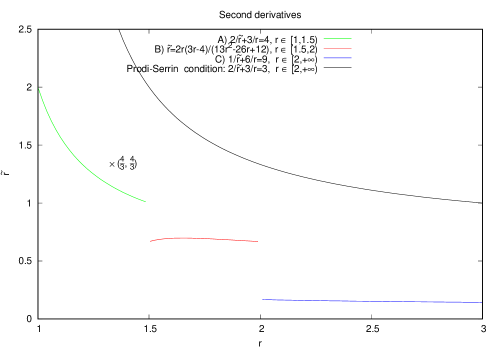
Let us precise some interpolations for the second derivatives. Namely, we gather all of these results in the below graphic, we draw the links between and in the above statement: .
Corollary 3.
Let a Leray solution of (1.2), and if , and then as soon as
The equality case is not proved yet. The work of Lions [Lio96] and Vasseur et al. [Vas10], [VY21] get closer to this equality.
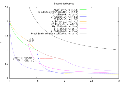
Proof of Corollary 3 and interpolation Figure 2.
The curves A), B) and C) are already proved by Theorem 1.
-
Curve D)
By interpolation, from and we compute******See (2.18) further. that with
which equivalently writes .
We have .
In the following we set
-
Curve E)
We interpolate between the curve A) at the point and the end of the curve B) at the point , thanks to identity (2.18)
(4.1) As we can see the best result is at the point given by (1.5), let us interpolate from this point.
- Curve F)
-
Curve G)
We interpolate from to thanks to identity (2.18)
-
Curve H)
We interpolate from to the end of curve C) thanks to (2.18):
We interpolate from to the end of curve C) thanks to (2.18):
We interpolate from to the end of curve C) thanks to (2.18):
∎
4.2 First derivatives
We can also perform the same reasoning for , directly from Corollary 3 and Sobolev embedding
Corollary 4.
Let a Leray solution of (1.2), if for any , and such that then as soon as
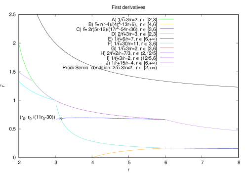
Proof of Corollary 4 and interpolation Figure 3.
The curves A) and B)
are already proved by Theorem 1.
By Gagliardo-Nirenberg interpolation, we can derive the case from the case , indeed the corresponding Lebesgue space for matches with the Lebesgue space for .
-
Curve C)
We get for any , the corresponding relation from Theorem 1,
-
Curve D)
The corresponding case for is and,
-
Curve E)
If , the corresponding case for is and from Theorem 1,
-
Curve F)
The corresponding case for is ,
Let us remark that .
-
Curve G)
For any , we interpolate the curve A) at to the curve C) at , and from (2.18) we get
Let us remark that we have .
Next, we derive from Sobolev embedding and Corollary 3,
-
Curve H)
, if
-
Curve I)
, if
-
Curve J)
,
Gathering the upper curves in the current proof yields the corollary. ∎
5 Weighted Lebesgue space in time
In the analysis of the solution of (1.2), in a mild formulation, a control of time integral with singularity might be directly useful.
Theorem 5.
Let a Leray solution of (1.2), if for all , , and , and such that
then
| (5.1) |
if
| (5.2) |
and if (with for ).
Also, if and , or , we can suppose that .
Remark 5.
However, by replacing suitably the parameters , , , we get the constraint which is a poorer result than the Leray estimates (1.4). By a homogeneity argument, there is no hope to get substantially better estimates without getting ride of the bilinear contribution (disappearing with the energy method).
We can postulate that for any ,
if , which is negative if .
The main problem to by-product our analysis in order to prove this result, is how to handle with a time singularity of order , with .
Another difficulty is to find the appropriate Lebesgue space in a such case. For instance, it seems that we should consider , for , to obtain the same results as in Theorem 5 by Gagliardo-Nirenberg estimates in three dimensions.
The analysis is similar to the one performed for Theorem 5, the main change lies in the non-linear contribution . We do not use neither Lemma 1 nor Hardy-Littlewood-Sobolev inequality (2.19), but instead we take advantage of the double time integrals.
5.1 Case
Lemma 6.
For all , and , , if
Furthermore, if , we can suppose that .
Remark 6.
Still, this result allows to handle with the Lebesgue space , with arbitrary big.
Proof of Lemma 6.
By the usual Duhamel formula around the heat equation, we get, for any
Next, by Minkowski inequality, for any ,
The last term in the r.h.s comes from the incompressible property of (2.4) (i.e. ), and by the convolution property of the heat semi-group.
From Young inequality for the convolution with such that
| (5.3) |
and by Minkowski inequality,
| (5.4) | |||||
The Leray operator disappears in the first inequality thanks to a Calderón-Zygmund estimate.
Importantly, we can already remark that the term is integrable if .
Recalling that, from Gagliardo-Nirenberg inequality,
| (5.5) |
Without looking at the time singularity in the r.h.s. of (3.3), we can choose , and in order to get this control in of , we can interpolate in the Lebesgue spaces,
| (5.6) |
with such that
in other words,
Let us also remark that , and .
That is to say, as lies in and that is in , we can see from (5.6), that is in . Specifically, for any , from (5.6), we derive
| (5.7) |
Let us go back to (3.3), for , , and for small enough (specified further),
We have the useful integral result.
Proposition 6.
For all and
Hence, for all and ,
If ,
Next, by Hölder inequality, with the conjugate value ,
| (5.8) | |||||
which is finite, see (5.7), if
namely
In that case, we have .
∎
Remark 7.
We have to pay attention, if , we cannot suppose that , implying a non integrable singularity in time, as we have to impose to use Proposition 6.
5.1.1 Final control of
Lemma 7.
For all , and , , if
Proof of Lemma 7.
Let us recall interpolation inequality of Sobolev spaces by Brezis Mirunescu [BM18], for and :
such that
That is to say, we obtain
| (5.9) |
and
| (5.10) |
Hence, we get with the same integral permutation performed in Section 5.1,
by interpolation inequality (2.20) and by Gagliardo-Nirenberg inequality , so
by Proposition 6 as soon as and .
Ultimately, to derive a inequality with from our analysis with , it suffices to use a Calderòn-Zygmund estimate from the Biot and Savart representation , available in the incompressible case.
Actually, we do not take into account (), because in such a case it is not direct to upper bound by ; unlike for . Furthermore, we even have .
Remark 8.
As we already said in Remark 6, we have to exploit more the regularisation by the heat kernel in order to get controls involving more regularity than in (1.3) and (1.4). This is what is done in the next section, where we differentiate once more Duhamel formula (3.23); yet we have to be careful on the regularity of the Sobolev norm considered in a way that the time singularity remains integrable.
∎
5.2 Control of
Lemma 8.
For all , and , if
Proof.
Let us start again the analysis of from the proof of Lemma 5. We recall the representation of ,
Still by interpolation of Brezis Mirunescu and in the Lebesgue spaces, for
| (5.12) |
by Gagliardo-Nirenberg interpolation inequality, and where we recall identities (5.9) and (5.10)
With the same argument performed in (3.39), and from (5.2), but with the same integral permutation in time performed in Proposition 6, we derive
Next, by interpolation inequality (5.12),
By Hölder inequality, we have
which is finite if , implying that, for any ,
and if the following condition is satsified,
as .
In fine, once again, to get an inequality with instead of , we can use a Calderòn-Zygmund inequality for the Biot and Savart representation. ∎
References
- [Alb00] G. Alberti. Some remarks about a notion of rearrangement. Ann. Scuola Norm. Sup. Pisa Cl. Sci. (4), 29(2):457–472, 2000.
- [BCD11] H. Bahouri, J.-Y. Chemin, and R. Danchin. Fourier analysis and nonlinear partial differential equations, volume 343 of Grundlehren der Mathematischen Wissenschaften [Fundamental Principles of Mathematical Sciences]. Springer, Heidelberg, 2011.
- [BLR04] H. Berestycki and T. Lachand-Robert. Some properties of monotone rearrangement with applications to elliptic equations in cylinders. Math. Nachr., 266:3–19, 2004.
- [BM18] H. Brezis and P. Mironescu. Gagliardo-Nirenberg inequalities and non-inequalities: the full story. Ann. Inst. H. Poincaré C Anal. Non Linéaire, 35(5):1355–1376, 2018.
- [Bre99] H. Brezis. Analyse fonctionnelle. Dunod, 1999.
- [Car95] G. Carbou. Unicité et minimalité des solutions d’une équation de Ginzburg-Landau. Ann. Inst. H. Poincaré C Anal. Non Linéaire, 12(3):305–318, 1995.
- [Cha92] D. Chae. Some a priori estimates for weak solutions of the -D Navier-Stokes equations. J. Math. Anal. Appl., 167(1):236–244, 1992.
- [Che98] J.-Y. Chemin. Perfect incompressible fluids, volume 14 of Oxford Lecture Series in Mathematics and its Applications. The Clarendon Press, Oxford University Press, New York, 1998. Translated from the 1995 French original by Isabelle Gallagher and Dragos Iftimie.
- [Con90] P. Constantin. Navier-Stokes equations and area of interfaces. Comm. Math. Phys., 129(2):241–266, 1990.
- [Con91] P. Constantin. Remarks on the Navier-Stokes equations. In New perspectives in turbulence (Newport, RI, 1989), pages 229–261. Springer, New York, 1991.
- [DF02] C. R. Doering and C. Foias. Energy dissipation in body-forced turbulence. J. Fluid Mech., 467:289–306, 2002.
- [Dra87] S. S. Dragomir. The Gronwall type lemmas and applications, volume 29 of Monografii Matematice (Timişoara) [Mathematical Monographs (Timişoara)]. Universitatea din Timişoara, Facultatea de Ştiinţe ale Naturii, Secţia Matematică, Timişoara, 1987.
- [Duf90] G. F. D. Duff. Derivative estimates for the Navier-Stokes equations in a three-dimensional region. Acta Math., 164(3-4):145–210, 1990.
- [Fef06] C. L. Fefferman. Existence and smoothness of the Navier-Stokes equation. In The millennium prize problems, pages 57–67. Clay Math. Inst., Cambridge, MA, 2006.
- [FGT81] C. Foiaş, C. Guillopé, and R. Temam. New a priori estimates for Navier-Stokes equations in dimension . Comm. Partial Differential Equations, 6(3):329–359, 1981.
- [Hen81] D. Henry. Geometric theory of semilinear parabolic equations, volume 840 of Lecture Notes in Mathematics. Springer-Verlag, Berlin-New York, 1981.
- [Kaw85] B. Kawohl. Rearrangements and convexity of level sets in PDE, volume 1150 of Lecture Notes in Mathematics. Springer-Verlag, Berlin, 1985.
- [Lad69] O. A. Ladyzhenskaya. The mathematical theory of viscous incompressible flow. New York - London - Paris: Gordon and Breach Science Publishers. XVIII, 224 p. (1969)., 1969.
- [Ler34] J. Leray. Sur le mouvement d’un liquide visqueux emplissant l’espace. Acta Math., 63:193–248, 1934.
- [Lio96] P.L. Lions. Mathematical Topics in Fluid Mechanics: Volume 1: Incompressible Models. Mathematical Topics in Fluid Mechanics. Oxford University Press, Incorporated, 1996.
- [LL01] E. H. Lieb and M. Loss. Analysis, volume 14 of Graduate Studies in Mathematics. American Mathematical Society, Providence, RI, second edition, 2001.
- [LR02] P.-G. Lemarié-Rieusset. Recent developments in the Navier-Stokes problem. CRC Press, 2002.
- [LR07] P. G. Lemarié-Rieusset. The Navier-Stokes equations in the critical Morrey-Campanato space. Rev. Mat. Iberoam., 23(3):897–930, 2007.
- [LR16] P. G. Lemarié-Rieusset. The Navier-Stokes problem in the 21st century. CRC Press, Boca Raton, FL, 2016.
- [MB02] A. J. Majda and A. L. Bertozzi. Vorticity and incompressible flow, volume 27 of Cambridge Texts in Applied Mathematics. Cambridge University Press, Cambridge, 2002.
- [MPcF91] D. S. Mitrinović, J. E. Peˇcarić, and A. M. Fink. Inequalities involving functions and their integrals and derivatives, volume 53 of Mathematics and its Applications (East European Series). Kluwer Academic Publishers Group, Dordrecht, 1991.
- [Ose11] C. W. Oseen. Sur les formules de green généralisées qui se présentent dans l’hydrodynamique et sur quelquesunes de leurs applications. Acta Math., 34(1):205–284, 1911.
- [Ose12] C. W. Oseen. Sur les formules de Green généralisées qui se présentent dans l’hydrodynamique et sur quelquesunes de leurs applications. Acta Math., 35(1):97–192, 1912.
- [Pro59] G. Prodi. Un teorema di unicità per le equazioni di Navier-Stokes. Ann. Mat. Pura Appl. (4), 48:173–182, 1959.
- [Ser62] J. Serrin. On the interior regularity of weak solutions of the Navier-Stokes equations. Arch. Rational Mech. Anal., 9:187–195, 1962.
- [Ste70] E. M. Stein. Singular integrals and differentiability properties of functions. Princeton university press, 1970.
- [Tao13] T. Tao. Localisation and compactness properties of the Navier-Stokes global regularity problem. Anal. PDE, 6(1):25–107, 2013.
- [Tar78] L. Tartar. Topics in nonlinear analysis, volume 13 of Publications Mathématiques d’Orsay 78. Université de Paris-Sud, Département de Mathématiques, Orsay, 1978.
- [Tem79] R. Temam. Navier-Stokes Equations: Theory and Numerical Analysis. Studies in mathematics and its applications. North-Holland, 1979.
- [Tri83] H. Triebel. Theory of function spaces, volume 78 of Monographs in Mathematics. Birkhäuser Verlag, Basel, 1983.
- [Vas10] A. Vasseur. Higher derivatives estimate for the 3D Navier-Stokes equation. Ann. Inst. H. Poincaré C Anal. Non Linéaire, 27(5):1189–1204, 2010.
- [VY21] A. Vasseur and J. Yang. Second derivatives estimate of suitable solutions to the 3D Navier-Stokes equations. Arch. Ration. Mech. Anal., 241(2):683–727, 2021.