FedRAV: Hierarchically Federated Region-Learning for Traffic Object Classification of Autonomous Vehicles

Abstract

The emerging federated learning enables distributed autonomous vehicles to train equipped deep learning models collaboratively without exposing their raw data, providing great potential for utilizing explosively growing autonomous driving data. However, considering the complicated traffic environments and driving scenarios, deploying federated learning for autonomous vehicles is inevitably challenged by non-independent and identically distributed (Non-IID) data of vehicles, which may lead to failed convergence and low training accuracy. In this paper, we propose a novel hierarchically Federated Region-learning framework of Autonomous Vehicles (FedRAV), a two-stage framework,which adaptively divides a large area containing vehicles into sub-regions based on the defined region-wise distance, and achieves personalized vehicular models and regional models. This approach ensures that the personalized vehicular model adopts the beneficial models while discarding the unprofitable ones. We validate our FedRAV framework against existing federated learning algorithms on three real-world autonomous driving datasets in various heterogeneous settings. The experiment results demonstrate that our framework outperforms those known algorithms, and improves the accuracy by at least 3.69%. The source code of FedRAV is available at: https://github.com/yjzhai-cs/FedRAV.

I Introduction

Autonomous Vehicles (AVs) have made significant progress in industry and academia in recent years. Advanced autonomous driving technology liberates humans from laboring driving experiences while also raising numerous research challenges and open questions. AVs are required to address high-dimensional scenarios, the combinations of vehicles, traffic lights, pedestrians, objects, and weather conditions, which seem rarely satisfied with the amount of fed training data. As a prospective resolution, federated learning (FL) [1, 2, 3, 4] incorporates clients to train a global model using the data collected separately and preserves clients’ privacy.

However, deploying FL for AVs is in the face of vehicles’ non-independent and identically distributed data (i.e. Non-IID, also known as heterogeneous data) [5, 6, 7], especially considering the complicated traffic environments and driving scenarios. For example, the data collected from highways, urban areas, rural areas, schools, coasts, and mountains vary significantly in their distributions. Intuitively, data acquired from a smaller region tend to have more similar distributions, such as the data collected from the vehicles passing the same traffic light tend to be similar. Based on this observation, a hierarchically Federated Region-learning framework of Autonomous Vehicles (FedRAV) is proposed in this paper to establish an FL framework to learn from vehicles in sub-regions of a much larger area. Realizing FedRAV can help AVs learn autonomous driving models based on data of a more IID distribution, where many challenges need to be addressed. For example, how should a large area be divided into sub-regions adaptively considering the data distribution? To address the challenge, a partitioning mechanism with one-shot communication is proposed in this paper, which divides the area of interest into sub-regions of different sizes based on the region-wise distance, achieving better IID data in each region.

Furthermore, how should the system learn a specialized model for each AV to fit its local driving data? In order to specialize the models learned in each AV, a personalization strategy via hypernetworks is proposed. FedRAV employs a designated hypernetwork to learn specialized mask vectors per vehicle and personalizes the vehicular model by using the mask vector to weight the models shared by vehicles within the same region. These mask vectors ensure that the specialized vehicular model adopts the beneficial models while discarding the unprofitable ones. Furthermore, the same hypernetwork design is also applied to different regions, which allows vehicles to learn a personalized vehicular model while simultaneously benefiting from the specialized regional model based on regional data. Therefore, the proposed framework can address the Non-IID problem of AVs’ data and train the learning model based on numerous vehicles navigating in different regions, which promotes better autonomous driving adapted for driving scenarios.

The contributions of the paper are mainly three-fold:

• We empirically demonstrate that the spatial distribution of vehicles’ collected data exhibits regional similarities and design a partitioning mechanism to divide large driving areas into sub-regions effectively.

• We propose a novel hierarchically Federated Region-learning framework of Autonomous Vehicles suitable for achieving federated learning of vehicles considering the Non-IID driving data. Our framework presents an effective personalization strategy, exploiting richer data of plentiful vehicles to train better personalized vehicular models while maintaining regional models.

• We evaluate the performance of FedRAV on three real-world autonomous driving datasets and open-access the source code of FedRAV to contribute to the community.

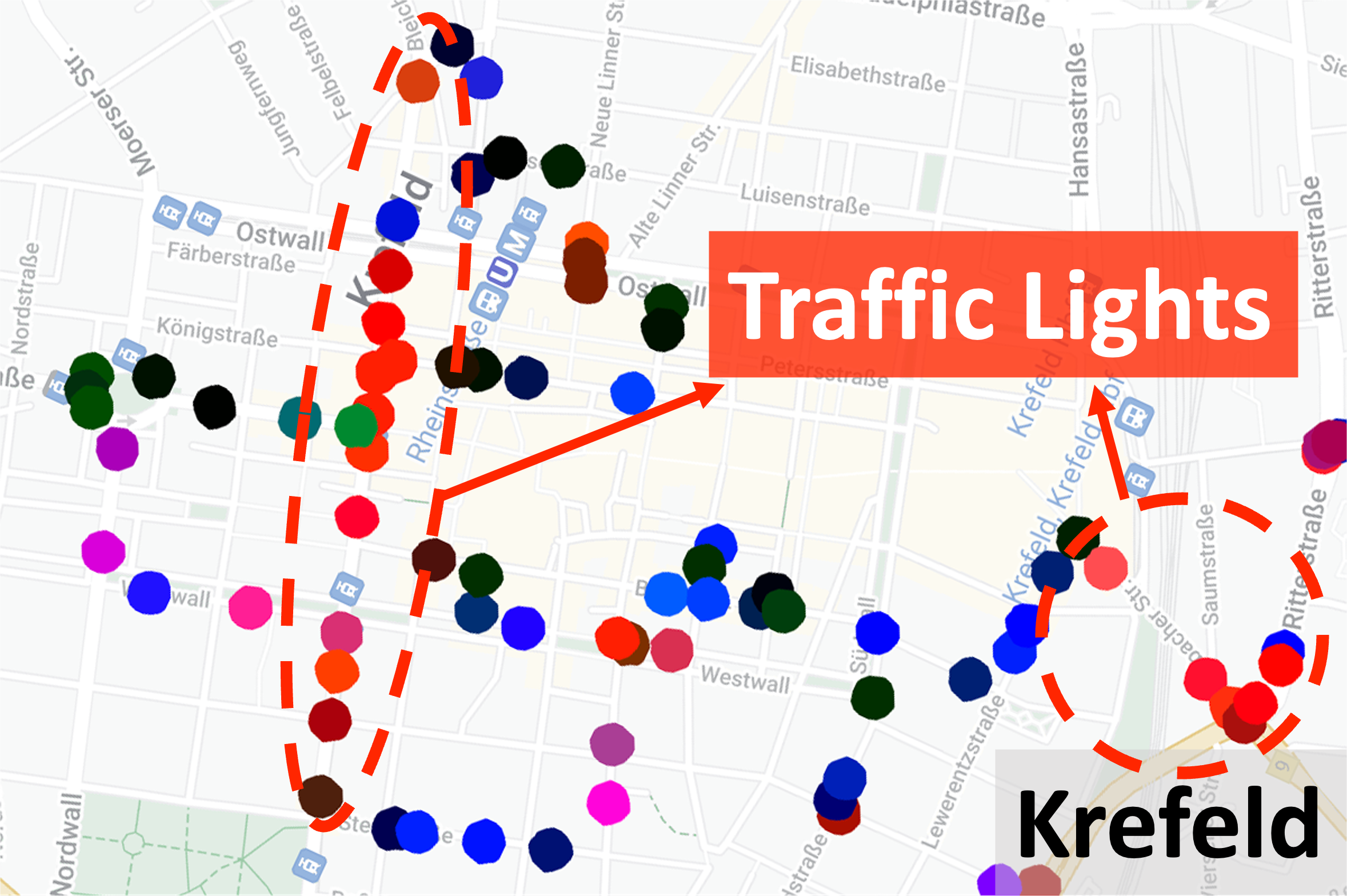
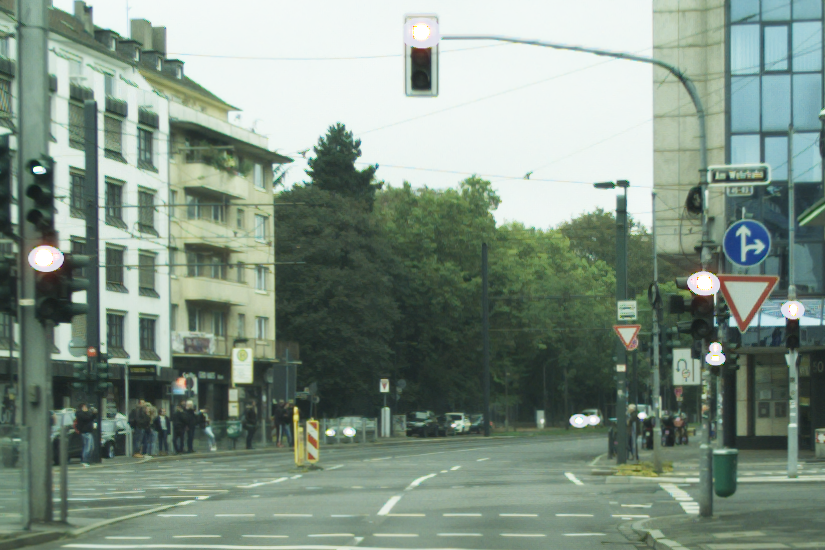
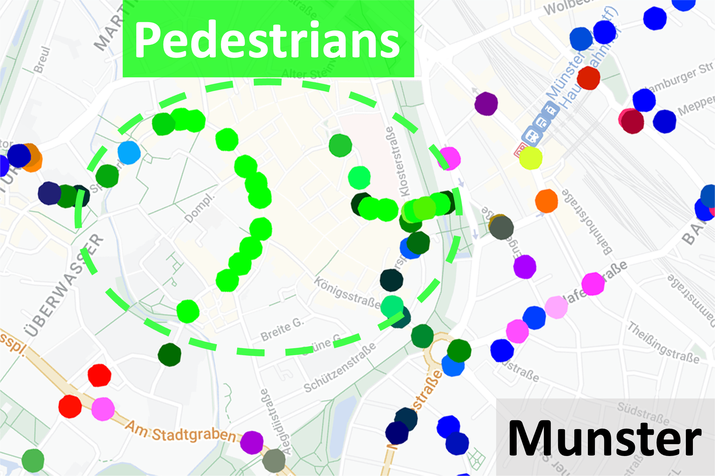
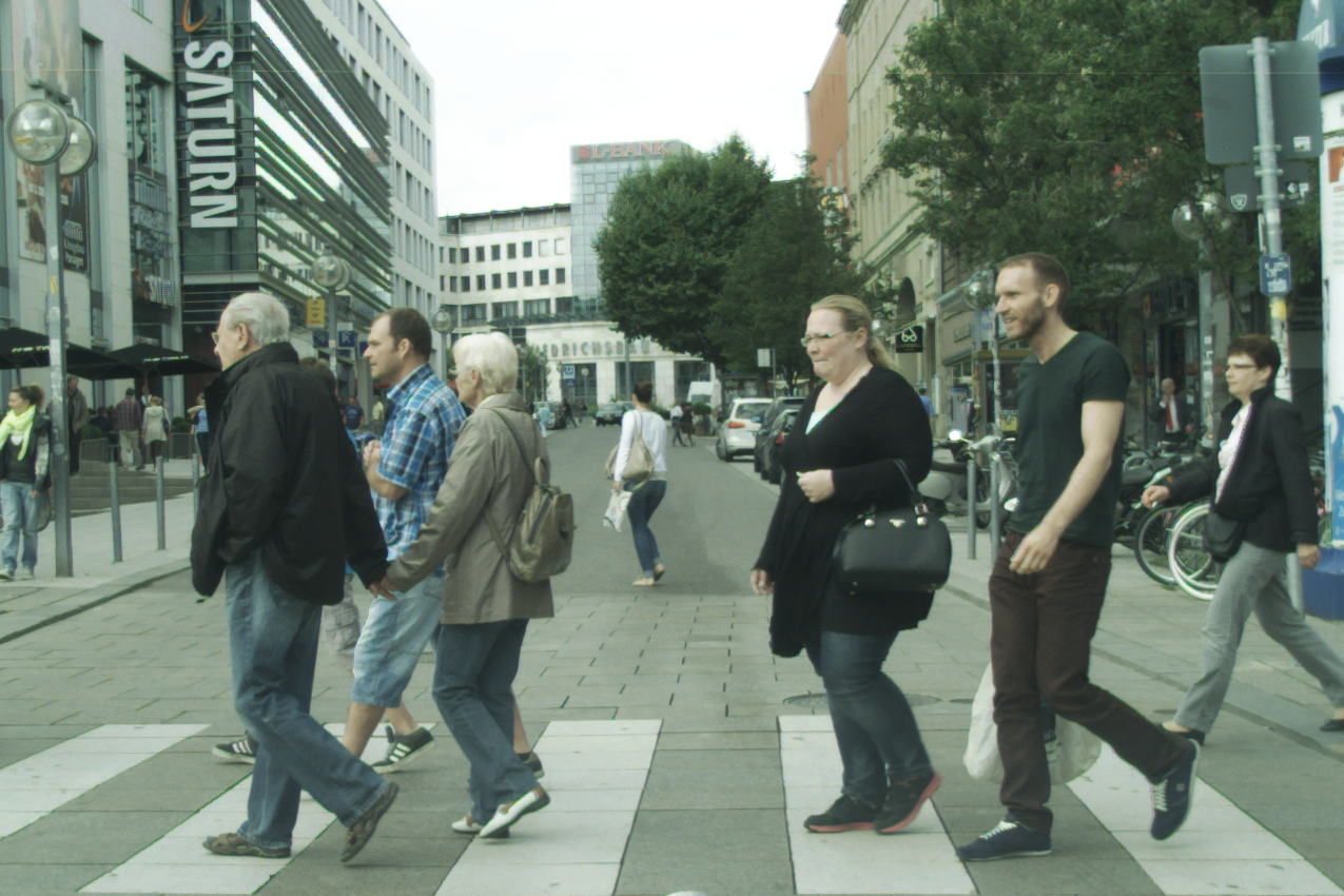
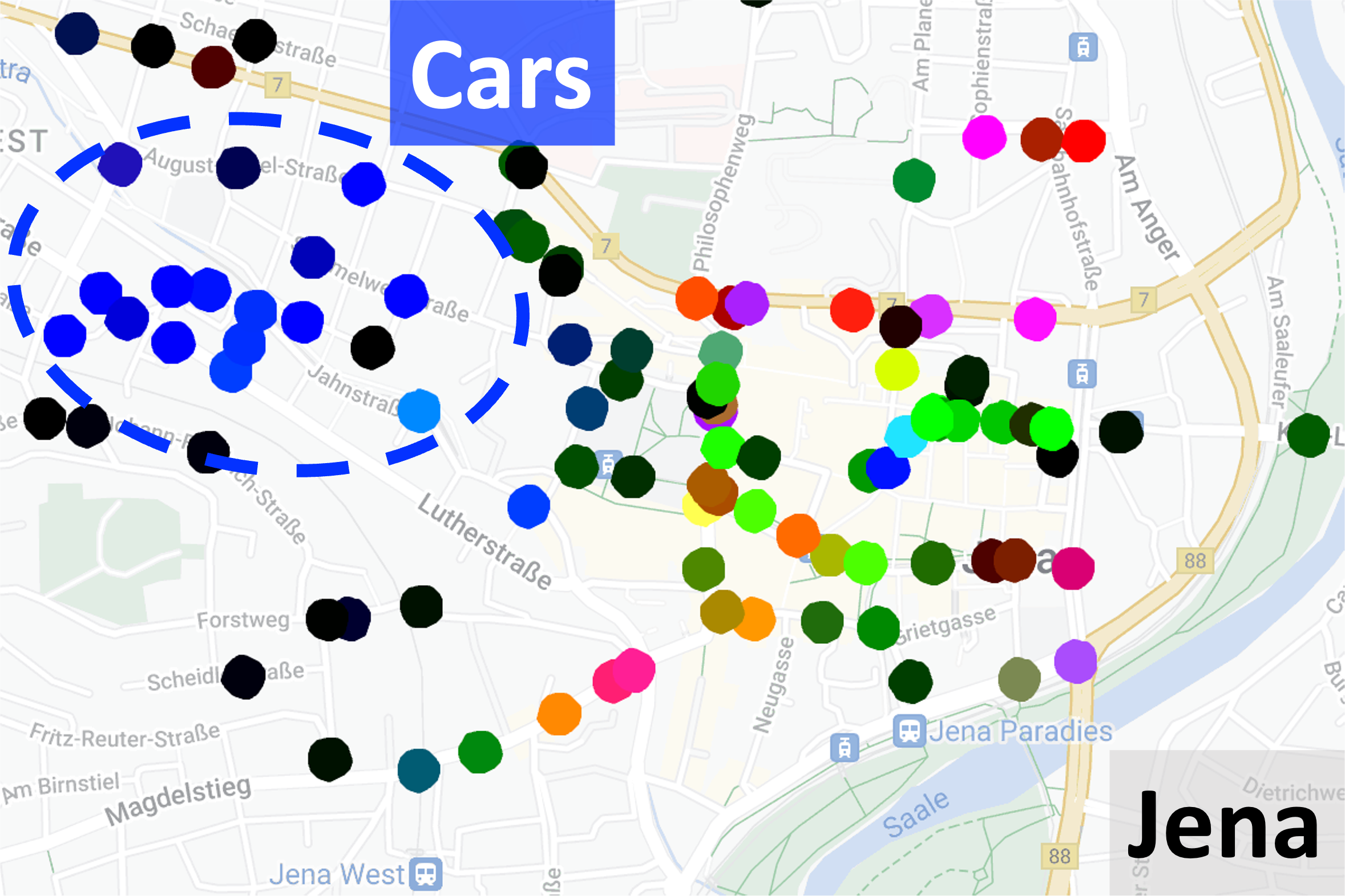
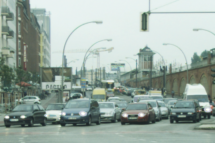
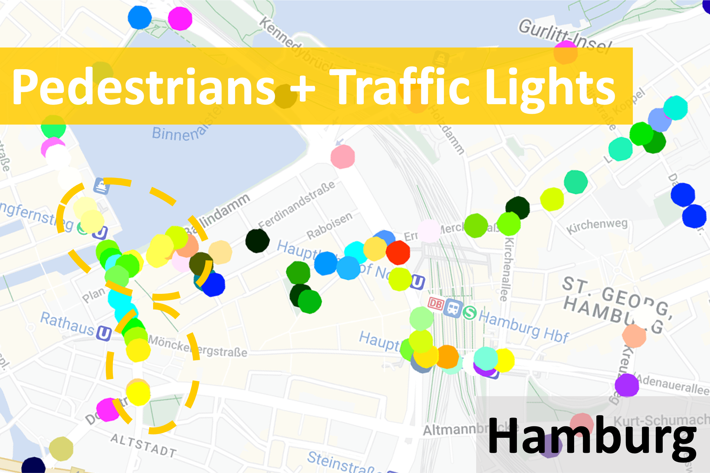
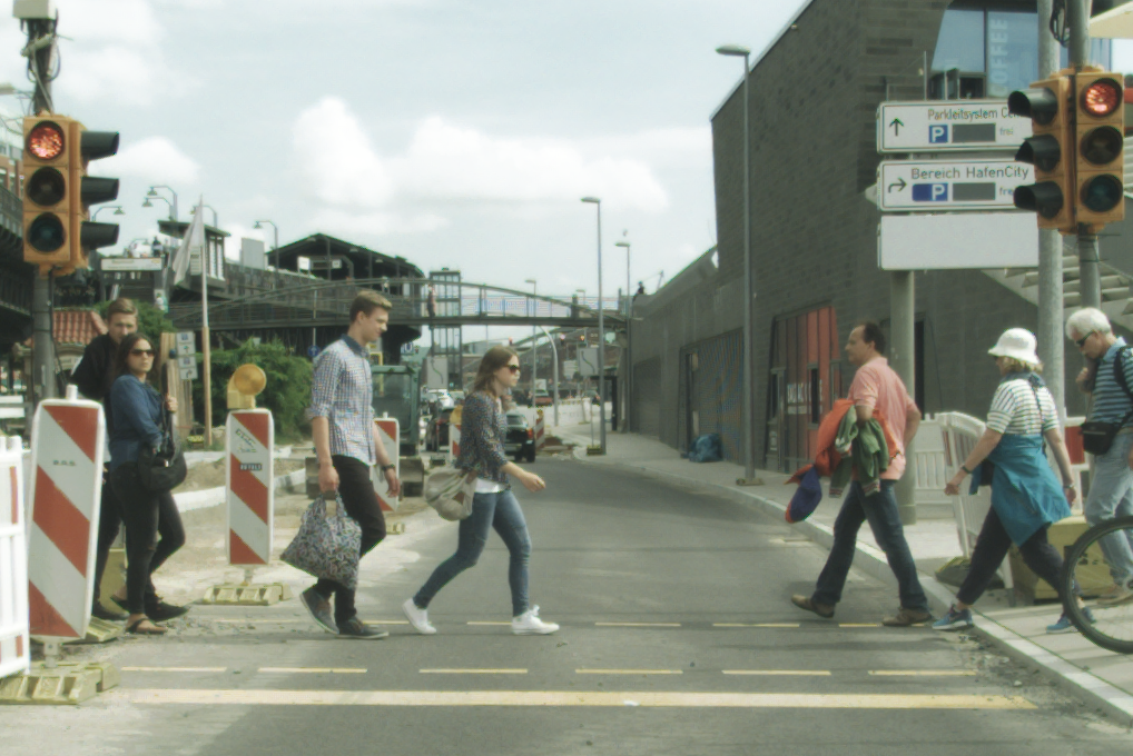
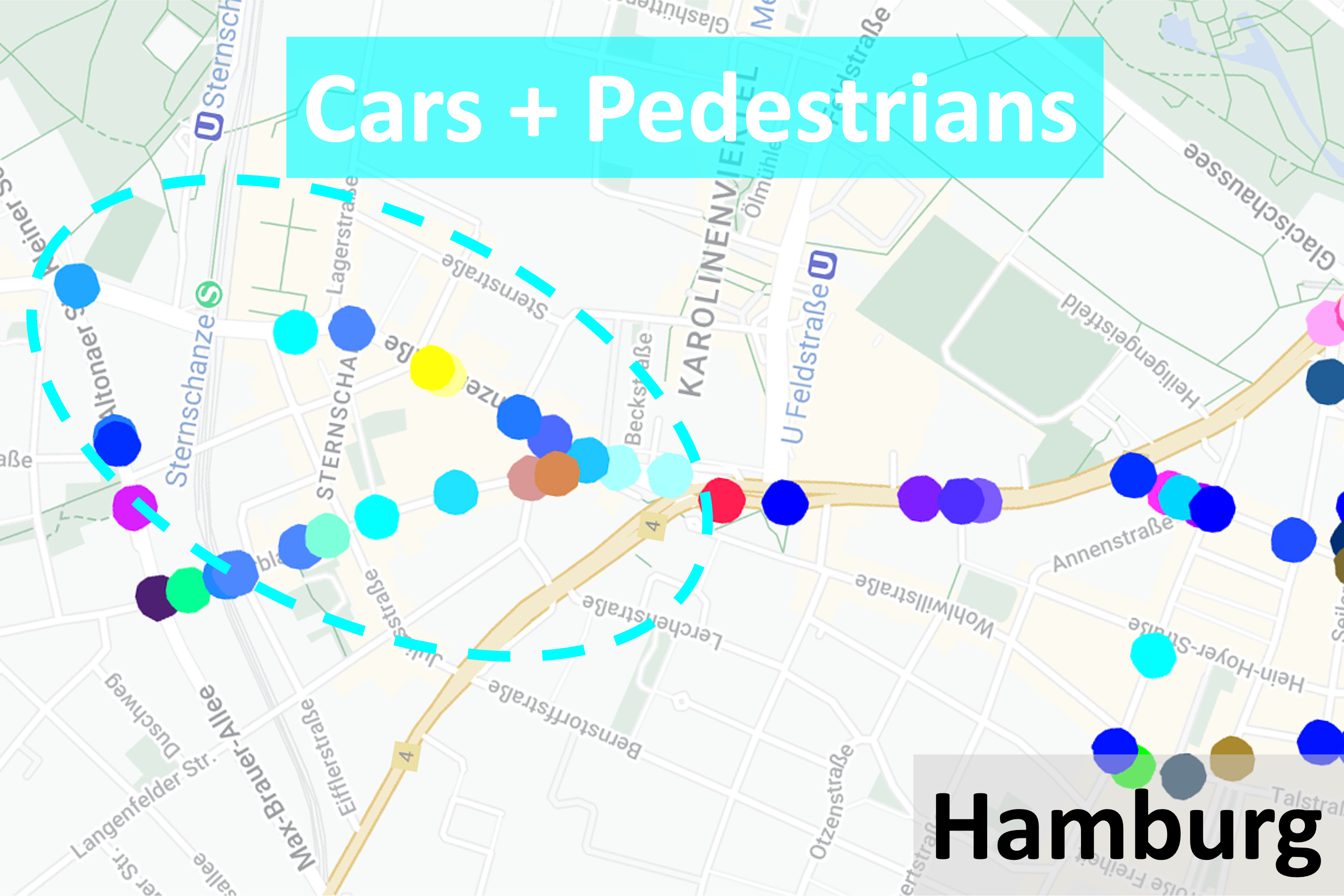
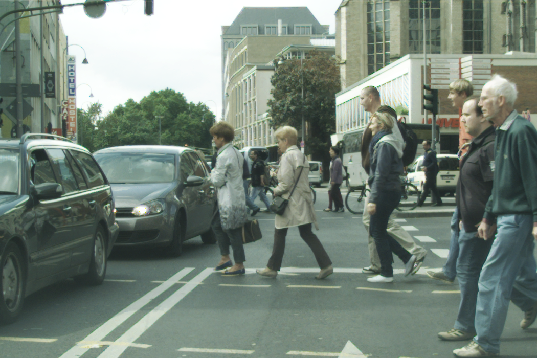
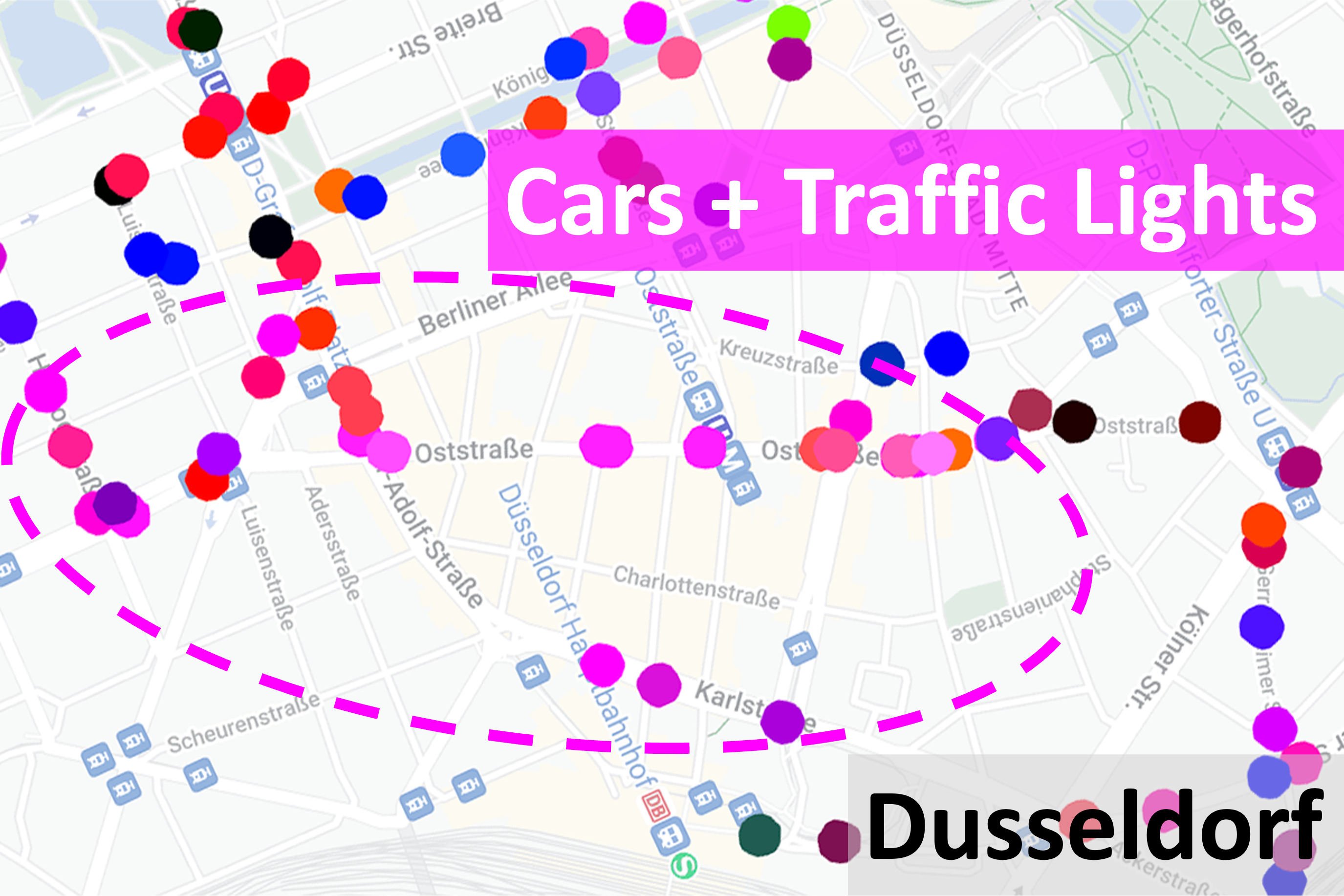
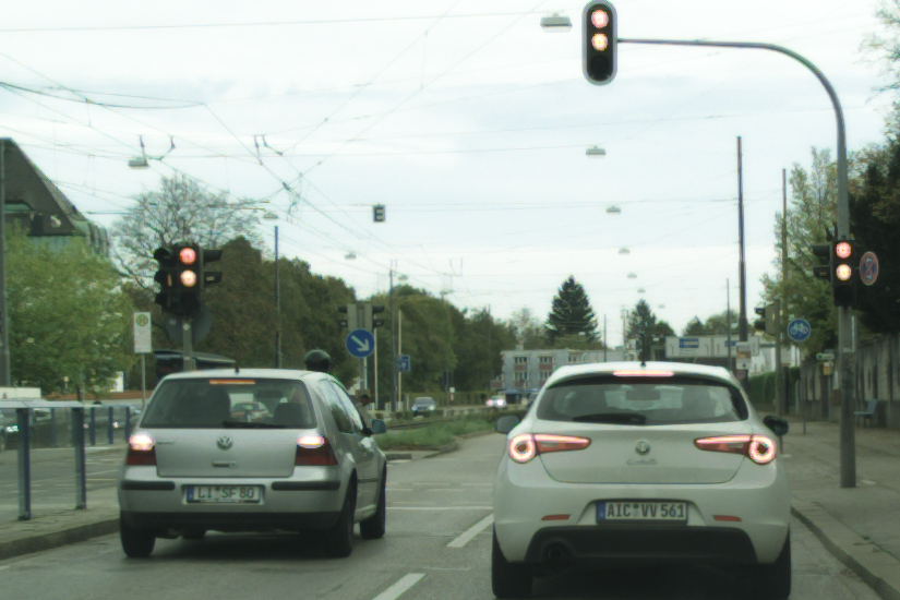
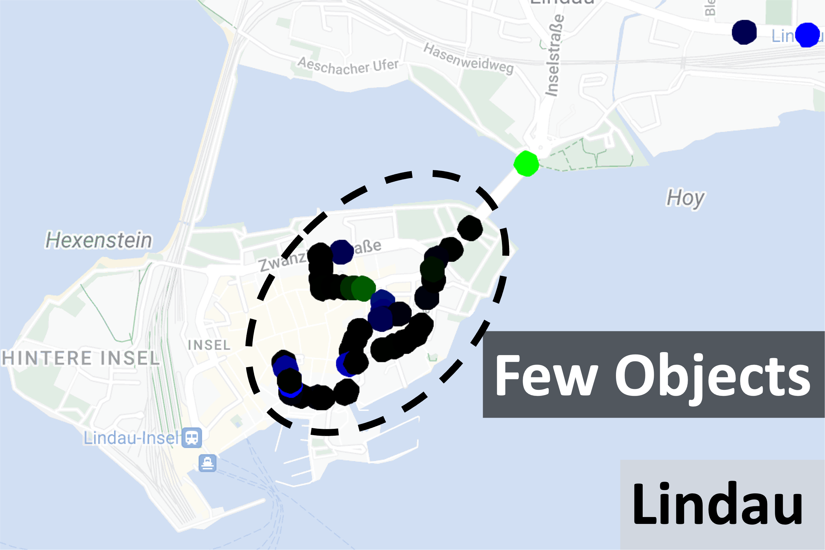
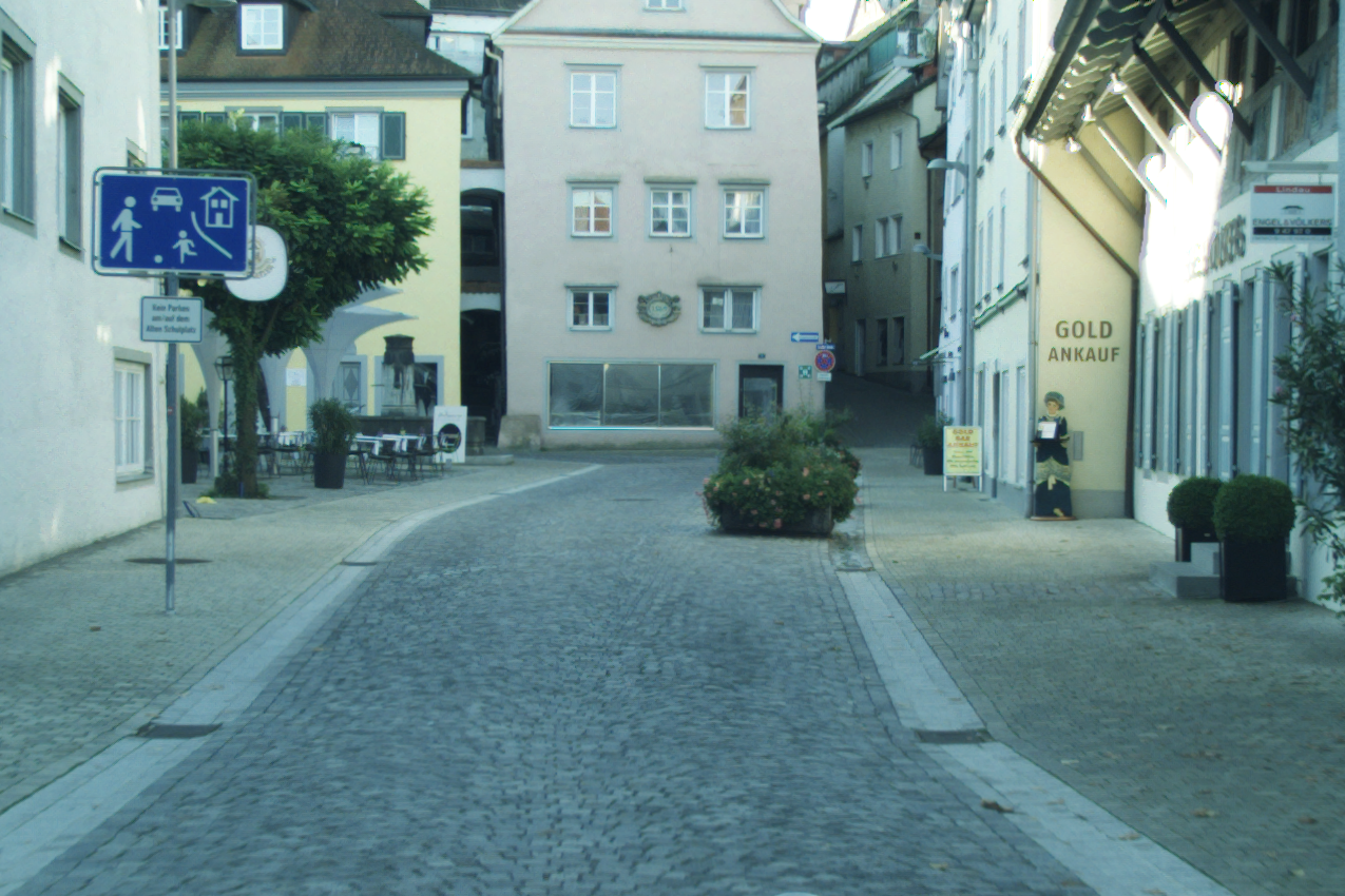
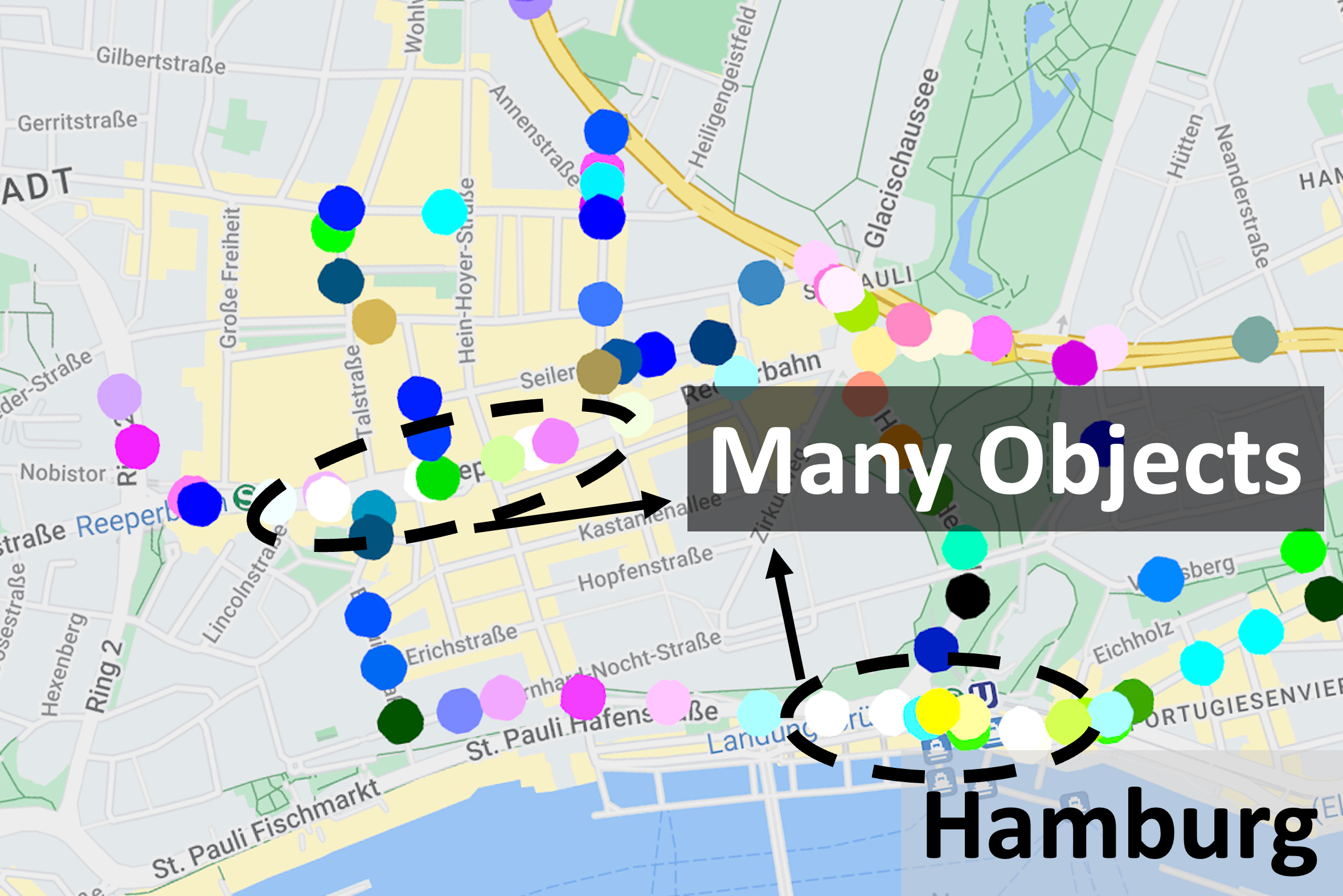
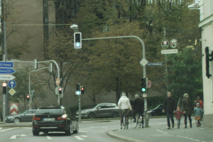
(c)

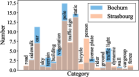
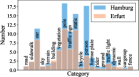
(a)                                                     (b)                                                     (d)

Figure 1: An example of regional similarities for the samples of Cityscapes on the map. (a) Traffic lights, pedestrians, and cars are dominant in certain-size regions, respectively. (b) All their binary combinations aggregate in certain-size regions. (c) There exist few objects or many objects in some regions. (d) The Significant difference in label distribution amongst the cities.

The remained paper are organized as following. Section II motivates this work with several case studies. Section III presents the partitioning mechanism. Section IV shows the design of the FedRAV framework. The experimental evaluations are presented in Section V. Section VI concludes this work.

II Preliminary Case Studies And Motivation

Before introducing a holistic framework, we motivate our work with a real-world example. We claim that the spatial distribution of vehicles’ collected data exhibits regional similarities, i.e., samples with similar label distributions tend to aggregate in nearby areas, forming regions. For example, urban and rural areas are usually divided into various sub-regions according to their diverse functions, i.e., schools, stadiums, commercial centers, transportation hubs, highways, country roads, and residential roads, etc. Vehicles traversing these regions tend to encounter more similar scenarios intra-regionally and encounter less similar scenarios inter-regionally. The claim is verified via analysis of realistic data from German cities in the following.

TABLE I: Color mapping table.

Color	$c_{i}^{r}$	$c_{i}^{g}$	$c_{i}^{b}$	Illustration of distribution
Red	255	0	0	Traffic Lights Dominant
Green	0	255	0	Pedestrians Dominant
Blue	0	0	255	Cars Dominant
Yellow	255	255	0	Abundant Traffic Lights & Pedestrians
Cyan	0	255	255	Abundant Cars & Pedestrians
Purple	255	0	255	Abundant Cars & Traffic Lights
Black	0	0	0	Three Categories Scarce
White	255	255	255	Three Categories Dominant

Specifically, the Cityscapes [8], a semantic segmentation dataset, consists of complex urban street scenes collected from $50$ cities of Germany, covering over $30$ different categories of traffic participants. The metadata of each image in the dataset provides the labels of different traffic participants and the spatial location of the collected data. We build the following visualization approach and choose three representative categories (i.e., traffic lights, pedestrians, and cars) to depict the data distribution of diverse categories. In order to intuitively depict the data distribution of samples on the map, the number of objects in each category of a sample is mapped to the color codes of RGB channels, where the colors red, green, and blue represent traffic lights $\omega_{1}$, pedestrians $\omega_{2}$, and cars $\omega_{3}$, respectively. The color code of RGB is an integer ranging from 0 to 255, and each color is denoted as a tuple $(c^{r},c^{g},c^{b})$ satisfying $\{c^{r},c^{g},c^{b}\}\in[0,255]$ and $\{c^{r},c^{g},c^{b}\}\in\mathcal{N}$. More formally, the red color code $c^{r}_{i}$ of sample $i$ is defined as a floor function,

$$\small c^{r}_{i}=\Big{\lfloor}\frac{l^{\omega_{1}}_{i}-\bar{l}^{\omega_{1}}_{\text{min}}}{\bar{l}^{\omega_{1}}_{\text{max}}-\bar{l}^{\omega_{1}}_{\text{min}}}\times 255\Big{\rfloor},$$ (1)

where $\bar{l}^{\omega_{1}}_{\text{max}}=\max\limits_{j}\{\bar{l}^{\omega_{1}}_{(j)}\}$ and $\bar{l}^{\omega_{1}}_{\text{min}}=\min\limits_{j}\{\bar{l}^{\omega_{1}}_{(j)}\}$. The subscript $j\in[M]$ denotes the $j$-th city among $M$ cities. $l^{\omega_{1}}_{i}$ represents the number of traffic lights in the sample $i$. $\bar{l}^{\omega_{1}}_{(j)}$ denotes the average quantity of traffic lights of the samples in the $j$-th city. The notations $\bar{l}^{\omega_{1}}_{\text{max}}$ and $\bar{l}^{\omega_{1}}_{\text{min}}$ represent the maximum and minimum average number of traffic lights of a sample among all $M$ cities.

Therefore, $c_{i}^{r}$ represents the richness of traffic light objects in the sample $i$. The larger value of $c_{i}^{r}$ depicts more abundant objects of traffic lights while the smaller value reflects the deficiency. $c_{i}^{r}$ is in value range $[0,255]$ and follows the rounding rule: if $c_{i}^{r}<0$, $c_{i}^{r}$ is rounded to $0$; if $c_{i}^{r}>255$, $c_{i}^{r}$ is rounded to $255$. Furthermore, $c_{i}^{g}$ and $c_{i}^{b}$ are defined similarly as, $c^{g}_{i}=\lfloor(l^{\omega_{2}}_{i}-\bar{l}^{\omega_{2}}_{\text{min}})/(\bar{l}^{\omega_{2}}_{\text{max}}-\bar{l}^{\omega_{2}}_{\text{min}})\times 255\rfloor$ and $c^{b}_{i}=\lfloor(l^{\omega_{3}}_{i}-\bar{l}^{\omega_{3}}_{\text{min}})/(\bar{l}^{\omega_{3}}_{\text{max}}-\bar{l}^{\omega_{3}}_{\text{min}})\times 255\rfloor$ respectively, following the same rounding rules as $c^{r}_{i}$. $c^{g}_{i}$ and $c^{b}_{i}$ depict the richness of pedestrians and cars in sample $i$.

As shown in Fig. 1, the distributions of samples are intuitively depicted on the Google Maps of cities via the above pre-defined color codes of the RGB channel. The codes reflect the label distribution of samples. Specifically, the Figs. 1(a)-(c) demonstrate some typical cases of the spatial distribution of samples in the Cityscapes dataset. The fundamental observation is that there exist 8 representative label distributions, whose details are summarized in Table I. It is observed that, certain patterns exist on the map, where samples with similar label distributions tend to aggregate in approximated regions.

The top two figures in Fig. 1(a) show regions where vehicles traverse multiple contiguous city blocks, where traffic lights or pedestrians are dominant in these blocks. The third figure shows a region where cars are crowded while traffic lights and pedestrians are insignificant. Fig. 1(b) demonstrates another three cases that two out of the three labels are dominant, where yellow regions show areas like harbors with many pedestrians and traffic lights, cyan regions show blocks with many cars and pedestrians appearing, and purple regions show popular commuting roads for cars together with many traffic lights but few pedestrians. In certain remote areas, there is scarcely any presence of traffic participants while in popular areas like tourist attractions, traffic participants of all three categories are abundant as shown in Fig. 1(c).

The collected vehicles’ data demonstrate dissimilarities across cities as shown in Fig. 1(d). The number of objects in 20 different labels is counted for different cities, leading to the comparison between Bochum and Strasbourg, and between Hamburg and Erfurt. In the first comparison, Bochum tends to have more poles, cars, and traffic lights since it is a greater city compared with the town Strasbourg, while Strasbourg tends to be more populous since many tourists aggregate locally. In the second comparison, as one of the greatest cities in Germany, Hamburg has more cars, poles, traffic signs and persons compared with Erfurt. Therefore, factors such as population, geography, culture, and economic development all affect the exhibited label distributions of samples collected in different cities, which substantiates that the spatial distributions of collected vehicle data do vary across regions. Based on the analysis above, we summarize the motivation below.

Motivation The spatial distribution of vehicles’ collected data exhibits visible regional similarities. The data distributions are more similar intra-regionally but less analogous inter-regionally. Therefore, partitioning regions adaptively is necessary for realizing FL in AVs.

III Regional Partitioning

Motivated by the regional similarities of the spatial distribution of AVs’ collected data, we introduce a novel distance in metric space to describe the similarity properties, which is referred to as Region-Wise Distance(RWD). Furthermore, we propose a new partitioning algorithm to divide large areas into sub-regions.

III-A Problem Formulation

We consider a vehicular network with $N$ AVs (a.k.a. clients) , $K$ region servers, and one central server. AVs distributed across $M$ cities or towns can traverse several city blocks along the roads. Each AV $i\in[N]$ has a local dataset $\mathcal{D}_{i}=\{x_{(i,j)},y_{(i,j)}\}^{|\mathcal{D}_{i}|}_{j=1}$ where $x_{(i,j)}$ is trainable image and $y_{(i,j)}$ is true label for the image classification task. $V_{i}=[v_{x},v_{y}]$ represents the coordinates of AV $i$. $L_{i}=[l^{1}_{i},l^{2}_{i},l^{3}_{i},\cdots,l^{m}_{i}]$ is the label vector of class distribution of $\mathcal{D}_{i}$ for $i$-th AV, where $l^{m}_{i}$ is the number of objects in $m$-th semantic category for AV $i$. We assume that a large area containing $N$ AVs is divided into $K$ sub-regions, i.e., $\{\mathcal{A}_{k}\}^{K}_{k=1}$ , and $U$ is the set of $k$ regional centroids. Let $\mathcal{X}=\{(V_{i},L_{i})\}^{N}_{i=1}$ denote a set of $N$ AVs. We formulate the problem of finding optimal regional structure $\{\mathcal{A}_{k}\}^{K}_{k=1}$ and regional centroids $U$ as Regional Structure Optimization (RSO) problem. The quantization error $\phi_{U}(\mathcal{X})$ is minimized, where

$$\small\textbf{P1}:\ \ \ \ \ \phi_{U}(\mathcal{X})=\sum_{x\in\mathcal{X}}\min_{u\in U}\textit{RWD}\left(x,u\right)^{2}$$ (2)

Subject to

$$\begin{array}[]{lc}\small\textit{RWD}\left(x,u\right)=||V_{x}-V_{u}||_{2}+\gamma\cdot[\zeta(C_{x}-C_{u})^{T}W\zeta(C_{x}-C_{u})]^{\frac{1}{2}}\\ \end{array}$$ (3)

$$\begin{array}[]{lc}\small|U|=K,|\mathcal{X}|=N&\\ \end{array}$$ (4)

The notation $\zeta(\cdot)$ represents the element-wise absolute value of the inside vector. The first constraint represents region-wise distance between AV $x$ and regional centroid $u$ where $\gamma$ is a hyperparameter controlling importance of the two components, $W\in\mathbb{R}^{m\times m}$ is a weight matrix and $C_{x}$ is $M$-relative abundance vector of AV $x$. Region-wise distance measures the similarity of data distributions for AVs in geographic space and embedding space of abundance. The abundance vector $C_{x}$ defines the relative richness of the categories in the local data of AV $x$. Specifically, we will discuss the details of the concepts of abundance and region-wise distance in Section III-B. The second constraint limits the number of regions and AVs. Now, the optimization problem aims to find $K$ subsets of $N$ AVs such that each AV can be assigned to a proper sub-region and data distributions are more similar intra-regionally. Thus, AVs in the same region $\mathcal{A}_{k}$ form a federation to jointly complete downstream learning tasks. $\phi_{U}(\mathcal{A}_{k})$ denotes the contribution of $\mathcal{A}_{k}\subset\mathcal{X}$ to the error. Then, $\delta(\mathcal{A}_{k})$ is used as an operator to indicate the mean coordinate of AVs indexed by $\mathcal{A}_{k}$, i.e., $\delta(\mathcal{A}_{k})=\frac{1}{|\mathcal{A}_{k}|}\sum_{i\in\mathcal{A}_{k}}V_{i}$ and use $\tau(\mathcal{A}_{k})$ to indicate the mean abundance of AVs indexed by $\mathcal{A}_{k}$, i.e., $\tau(\mathcal{A}_{k})=\frac{1}{|\mathcal{A}_{k}|}\sum_{i\in\mathcal{A}_{k}}C_{i}$.

III-B Region-Wise Distance

In a conventional partitioning setting, the large area is divided into sub-regions based on the $\ell_{2}$-norm of spatial locations of AVs. However, it does not consider similarities in label distribution across AVs. There is a trade-off between spatial location and label distribution in realistic situations. We tackle this problem via a control knob to combine spatial location with label distribution, which is described as follows.

Definition 1 (Spatial Distance). Assumed that $N$ AVs are located in the same Euclidean plane, and $V_{i}=[v_{x},v_{y}]$ is the coordinate of AV $i$. Then, the spatial distance between AV $i$ and AV $j$ is defined by,

$$\small d_{\text{spatial}}(i,j)=\|V_{i}-V_{j}\|_{2},\ \forall i,j\in[N].$$ (5)

Existing studies have used the cross-class $\ell_{2}$-norm distance to evaluate the similarity between label distributions. However, these measures are sensitive to changes in the number of objects of a particular class. Due to the absolute scale of these measures, regional partitioning may not benefit from them in realistic and challenging heterogeneous data distribution. Inspired by the visualization method in Section II, we extend the case to an M-dimensional label vector.

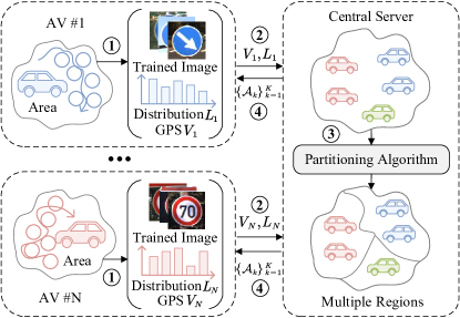
Figure 2: Illustration of partitioning mechanism. ① Collect data; ② upload coordinate $V$ and feature vector $L$; ③ divide areas into regions; ④ download regional structure $\{\mathcal{A}_{k}\}^{K}_{k=1}$.

Definition 2 ($M$-Relative Abundance). Given the label vector $L_{i}\in\mathbb{R}^{m}$ of local dataset $\mathcal{D}_{i}$ of AV $i$, the M-Relative Abundance of AV $i$ amongst all the AVs cross the $M$ cities is represented as $C_{i}=[c^{1}_{i},c^{2}_{i},c^{3}_{i}\cdots,c^{m}_{i}]$. Concretely, the abundance of $m$-th category $c^{m}_{i}$ is defined as,

$$\small c^{m}_{i}=\Big{\lfloor}\frac{l_{i}^{m}-\bar{l}_{\text{min }}^{m}}{\bar{l}_{\text{max }}^{m}-\bar{l}_{\text{min }}^{m}}\times 255\Big{\rfloor},$$ (6)

where we let $\bar{l}^{m}_{\text{max}}=\max\limits_{j}\{\bar{l}^{m}_{(j)}\}$ and $\bar{l}^{m}_{\text{min}}=\min\limits_{j}\{\bar{l}^{m}_{(j)}\}$. The subscript $j\in[M]$ denotes the $j$-th city among $M$ cities. $l^{m}_{i}$ represents the number of $m$-th category in the AV $i$. $\bar{l}^{m}_{(j)}$ denotes the average quantity of $m$-th category of all AVs in the $j$-th city. The notations $\bar{l}^{m}_{\text{max}}$ and $\bar{l}^{m}_{\text{min}}$ represent the maximum and minimum average number of $m$-th category of a AV among all $M$ cities, respectively. Specifically, Eq.(6). follows the same rounding rules as Eq.(1). Ranging from 0 to 255, $c^{m}_{i}$ demonstrates the relative abundance of category $m$ for AV $i$.

Definition 3 (Label Distance). Meanwhile, the label distance is defined by,

$$\small d_{\text{label}}(i,j)=\|C_{i}-C_{j}\|_{2},\ \forall i,j\in[N].$$ (7)

It presents a geometrical evaluation in embedding space of $M$-relative abundance vector. The generic form of the distance is given as follows,

$$\small d_{\text{label}}(i,j)=[\zeta(C_{i}-C_{j})^{T}W\zeta(C_{i}-C_{j})]^{\frac{1}{2}},\ \forall i,j\in[N],$$ (8)

where $W\in\mathbb{R}^{m\times m}$ is a weight matrix satisfying $W_{ij}\geq 0$. Here, we let $W=I$, which means that all categories are equally essential.

In order to obtain a optimal regional structure satisfying data similarities, we propose to apply region-wise distance to the optimization problem P1. As discussed earlier, a key challenge here is to achieve trade-off between spatial locations and label distribution. Therefore, a control knob $\gamma\in[0,1]$ is proposed to balance the spatial distance and label distance.

Definition 4 (Region-Wise Distance). Region-Wise Distance between AV $i$ and AV $j$ is defined by,

$$\small\textit{RWD}(i,j)=||V_{i}-V_{j}||_{2}+\gamma\cdot[\zeta(C_{i}-C_{j})^{T}W\zeta(C_{i}-C_{j})]^{\frac{1}{2}},$$ (9)

where $\forall i,j\in[N]$ and $\gamma$ is adjustable hyperparameter.

III-C Partitioning Mechanism

Our partitioning mechanism follows a client-server paradigm with one-shot communication, as shown in Fig. 2. The mechanism’s crux is thoroughly capturing the similarity between AVs by computing the region-wise distance. Therefore, multiple AVs are required to send their coordination $V$ and label vector $L$ to a central server. On the server side, we execute a partitioning algorithm to divide large areas of interest into sub-regions and send regional structure $\{\mathcal{A}_{k}\}^{K}_{k=1}$ back to AVs.

Specifically, the P1 is analogous to the Euclidean Clustering Problem, which is unfortunately NP-hard even for $K=2$. Due to NP-hardness, no polynomial-time algorithm exists unless P equals NP. Lloyd proposed a simple and fast heuristic called Lloyd’s algorithm[9] that begins with $K$ arbitrary initial solution and iteratively converges to a locally optimal solution. However, Lloyd’s algorithm is susceptible to improper initialization. K-Means++ seeding[10] can provide provably good initialization with $8(lnK+2)$-approximation to the global optimum in expectation. Inspired by the prior works, we propose a novel partition algorithm to solve P1 as shown in Algorithm 1. The algorithm first samples an initial centroid uniformly at random from the set of AVs $\mathcal{X}$ and adaptively samples $K-1$ additional centroids using seeding steps (lines 1-4). In each seeding iteration, the AV $x\in\mathcal{X}$ is added to the set of already sampled centroids $U$ with probability $\frac{\phi_{U}(\{x\})}{\phi_{U}(\mathcal{X})}$ where $\phi_{U}(\{x\})$ is the shortest region-wise distance from AV $x$ to the closest centroid that the Algorithm 1 has chosen. Then, the algorithm will use region-wise distance as a metric to repeat the standard Lloyd’s steps (lines 5-8) until a proper regional structure is found.

1

Input: A set $\mathcal{X}$ of $N$ AVs, number of regions $K>0$, control knob $0\leq\gamma\leq 1$, weight matrix $W\in\mathbb{R}^{m\times m}$.

2

Output: regional structure $\{\mathcal{A}_{k}\}^{K}_{k=1}$ and regional centroids $U$.

3

4$U\leftarrow$ Sample an AV uniformly at random from $\mathcal{X}$

5while $|U|<K$ do

6       Sample $x\in\mathcal{X}$ with probability $\frac{\phi_{U}(\{x\})}{\phi_{U}(\mathcal{X})}$ $\triangleright$ Sample centroids

7      $U\leftarrow U\cup\{x\}$

8

9while $U$ is not stable do

10       $\mathcal{A}_{r}\leftarrow\{i:\textit{RWD}(i,r)^{2}\leq\textit{RWD}(i,s)^{2},\forall s\in U\}$

11      $V_{r}=\delta(\mathcal{A}_{r})$ , $C_{r}=\tau(\mathcal{A}_{r})$

12      Update $U$ by $(V_{r},C_{r})$ $\triangleright$ Update centroids

13

14return $\{\mathcal{A}_{k}\}^{K}_{k=1}$ and $U$

Algorithm 1 Regional Partitioning Algorithm

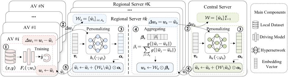
Figure 3: An overview of FedRAV Framework. The main operations consist of: ① local training on private dataset $\mathcal{D}$ ; ② upload model update $\Delta\boldsymbol{w}$; ③ model personalization; ④ intra-region model aggregation; ⑤ download personalized model $\boldsymbol{\tilde{w}}$.

IV Federated Region-learning Framework of Autonomous Vehicles (FedRAV)

In this section, we present the FedRAV framework that learns driving models via device-edge-cloud communication.

IV-A Problem Formulation

In the standard FL setting, the optimization objective aims to find a single global model. It assumes the global model is capable of learning empirical knowledge for every case. However, the prior studies like [5] have proved that a single model may not fit parameter space from models of multiple users. The leading cause of the problem is that local data heterogeneity leads to discrepant model parameter space. More specifically, the discrepant model disturbs the inter-client knowledge transfer. Therefore, to resolve these problems, we propose FedRAV framework that learns a personalized model for each AV and each region respectively.

The optimal regional structure $\{\mathcal{A}_{k}\}^{K}_{k=1}$ has been obtained in Section III. AV $i$ expects to learn personalized vehicular models $\boldsymbol{w}_{i}$ on private dataset $\mathcal{D}_{i}$. Thus, the local objective $F_{i}(\cdot;\cdot)$ of $i$-th vehicle is defined as,

$$\small F_{i}(\mathcal{D}_{i};\boldsymbol{w}_{i})\triangleq\frac{1}{|\mathcal{D}_{i}|}\sum_{j=1}^{|\mathcal{D}_{i}|}\ell\left(x_{(i,j)},y_{(i,j)};\boldsymbol{w}_{i}\right),$$ (10)

where $\ell(\cdot;\cdot)$ represents a user-defined loss function. In the training of each region $k$ in FedRAV, the vehicle-level joint optimization objectives are formulated as,

$$\small\textbf{P2}:\ \ \ \ \ \mathcal{W}_{k}^{*}=\operatorname*{arg\,min}_{\mathcal{W}_{k}}\frac{1}{\left|\mathcal{A}_{k}\right|}\sum_{i\in\mathcal{A}_{k}}{F_{i}}\left(\mathcal{D}_{i};\boldsymbol{w}_{i}\right),$$ (11)

where optimization variable $\mathcal{W}_{k}=[\boldsymbol{w}_{i}]_{i\in\mathcal{A}_{k}}$ represents the set of personalized vehicular models within the region $\mathcal{A}_{k}$. The optimization problem aims to find a set of personalized vehicular models fitting AVs’ parameter space, respectively. From a regional perspective, region $k$ also expects to learn personalized regional models $\boldsymbol{w}_{k}$ on union dataset $\mathcal{D}_{k}=\underset{i\in\mathcal{A}_{k}}{\cup}\mathcal{D}_{i}$. Specifically, AVs need not to transmit their own privacy-sensitive datasets to each region server or central server. Therefore, the regional objective $f_{k}$ is defined by,

$$\small f_{k}\left(\mathcal{D}_{k};\boldsymbol{w}_{k}\right)\triangleq\frac{1}{\left|\mathcal{D}_{k}\right|}\sum_{j=1}^{|\mathcal{D}_{k}|}\ell\left(x_{(k,j)},y_{(k,j)};\boldsymbol{w}_{k}\right).$$ (12)

We formulate region-level joint optimization objectives as,

$$\small\textbf{P3}:\ \ \ \ \ \mathcal{W}^{*}=\operatorname*{arg\,min}_{\mathcal{W}}\frac{1}{K}\sum^{K}_{k=1}{f_{k}}\left(\mathcal{D}_{k};\boldsymbol{w}_{k}\right),$$ (13)

where the optimization variable $\mathcal{W}=[\boldsymbol{w}_{k}]^{K}_{k=1}$ is the set of all the personalized regional models. Similarly, the optimization problem seeks to find a set of personalized regional models fitting parameter space related to regions.

IV-B Overview of FedRAV Framework

We now present our FedRAV framework that can resolve the above optimization problems P2 and P3 via hypernetworks. Specifically, hypernetworks are widely used in fields of natural language modeling and computer vision to generate model parameters for other neural network. Before delving into more detail, the overview of the federated optimization process is shown in Fig. 3. Concretely, the entire optimization process consists of the following three stages.

Federated Initialization. As shown in Fig. 3, each AV has a designated hypernetwork on the regional server side, and each region holds a corresponding hypernetwork on the central server side. Then, the hypernetwork $h(\boldsymbol{v};\boldsymbol{\varphi})$ is also a particular deep neural network that maintains a trainable embedding vector $\boldsymbol{v}$ as input and model parameter $\boldsymbol{\varphi}$. Before the FedRAV starts training, the embedding vector $\boldsymbol{v}$ and model parameter $\boldsymbol{\varphi}$ are initialized randomly. Given $\boldsymbol{v}$, the hypernetwork $h(\cdot;\cdot)$ can output the personalized mask vectors $\boldsymbol{\alpha}$ which can learn cross-client or cross-region information.

Local Personalization. Without loss of generality, suppose that AV $i$ executes local training with $\kappa_{1}$ iterations on the private dataset $\mathcal{D}_{i}$ and sends model update $\Delta\boldsymbol{w}_{i}$ to regional server $k$, as shown in the left part of Fig. 3. Then, the regional server $k$ can update the embedding vector $\boldsymbol{v}_{i}$ and model parameter $\boldsymbol{\varphi}_{i}$ via model update $\Delta\boldsymbol{w}_{i}$. Specifically, we will discuss the details of the update process in the next Section IV-C. As shown in the middle part of Fig. 3, the local personalization process of FedRAV takes place on the regional server $k$. Based on the updated embedding vector $\boldsymbol{v}_{i}$, the hypernetwork $h_{i}(\cdot;\cdot)$ can generate the new mask vectors $\boldsymbol{\alpha}_{i}$. FedRAV can obtain personalized vehicular models by using the mask vectors to weight the models shared by vehicles within the same region. Unlike FL approaches aggregate a single global model, FedRAV may fit each AV’s model parameter space, which gets rid of unprofitable models and ensures a better knowledge transfer.

Regional Personalization. We utilize the same trick of local personalization to personalize the regional model. Also, FedRAV provides a heuristic aggregation policy to obtain the regional model update $\Delta\boldsymbol{w}_{k}$, which is used to update the embedding vector $\boldsymbol{v}_{k}$ and hypernetwork model parameter $\boldsymbol{\varphi}_{k}$ in central server side, as shown in the right part of Fig. 3. We will discuss our heuristic policy for the intra-regional aggregation in Section IV-D. The details are summarized in Algorithm 2.

Input: Regional structure $\{\mathcal{A}_{k}\}^{K}_{k=1}$, local epochs $\kappa_{1}$, interval of intra-region aggregation $\kappa_{2}$, learning rate $\eta$, $\eta_{\boldsymbol{v}}$, $\eta_{\boldsymbol{\varphi}}$.

1

2

Output: Personalized vehicular models $\{\mathcal{W}_{k}\}^{k}_{k=1}$ and regional models ${\mathcal{W}}$.

3

4function CentralServerExecute:

5       Initialize $\mathcal{W}^{(t_{0})}=[\boldsymbol{\tilde{w}}^{(t_{0})}_{1},\cdots,\boldsymbol{\tilde{w}}^{(t_{0})}_{K}]$

6      for each round $t\in\{0,...,T-1\}$ do

7             for  each regional server $k=1,...,K$ in parallel do

8                   $\boldsymbol{\tilde{w}}^{(t+1)}_{k}\leftarrow\boldsymbol{\tilde{w}}^{(t)}_{k}+(\mathcal{W}^{(t)}\setminus\boldsymbol{\tilde{w}}^{(t)}_{k})\odot h_{k}(\boldsymbol{v}^{(t)}_{k};\boldsymbol{\varphi}^{(t)}_{k})$

9                  $\Delta\boldsymbol{w}_{k}=$ RegionUpdate($t$, $k$, $\boldsymbol{\tilde{w}}^{(t+1)}_{k},\mathcal{A}_{k}$)

10                  Update ${\mathcal{W}^{(t)}}$ according to $\Delta\boldsymbol{w}_{k}$

11                  $\boldsymbol{v}^{(t+1)}_{k}\leftarrow\boldsymbol{v}^{(t)}_{k}-\eta_{\boldsymbol{v}}\left(\nabla_{\boldsymbol{v}^{(t)}_{k}}\boldsymbol{\tilde{w}}^{(t+1)}_{k}\right)^{T}\Delta\boldsymbol{w}_{k}$

12                  $\boldsymbol{\varphi}^{(t+1)}_{k}\leftarrow\boldsymbol{\varphi}^{(t)}_{k}-\eta_{\boldsymbol{\varphi}}\left(\nabla_{\boldsymbol{\varphi}^{(t)}_{k}}\boldsymbol{\tilde{w}}^{(t+1)}_{k}\right)^{T}\Delta\boldsymbol{w}_{k}$

13            

14      

15      return personalized regional models ${\mathcal{W}^{(T-1)}}$

16

17function RegionUpdate($t$, $k$, $\boldsymbol{\tilde{w}}^{(t)}_{k}$, $\mathcal{A}_{k}$):

18       Initialize $\mathcal{W}^{(t)}_{k}=[\boldsymbol{\tilde{w}}^{(t)}_{i}]_{i\in\mathcal{A}_{k}}$ with $\boldsymbol{\tilde{w}}^{(t)}_{k}$

19      for each AV $i\in\mathcal{A}_{k}$ in parallel do

20             $\boldsymbol{\tilde{w}}^{(t+1)}_{i}\leftarrow\boldsymbol{\tilde{w}}^{(t)}_{i}+(\mathcal{W}^{(t)}_{k}\setminus\boldsymbol{\tilde{w}}^{(t)}_{i})\odot h_{i}(\boldsymbol{v}^{(t)}_{i};\boldsymbol{\varphi}^{(t)}_{i})$

21            $\Delta\boldsymbol{w}_{i}=$ AVUpdate($t$, $k$, $i$, $\boldsymbol{\tilde{w}}^{(t+1)}_{i}$)

22            Update ${\mathcal{W}^{(t)}_{k}}$ according to $\Delta\boldsymbol{w}_{i}$

23            $\boldsymbol{v}^{(t+1)}_{i}\leftarrow\boldsymbol{v}^{(t)}_{i}-\eta_{\boldsymbol{v}}\left(\nabla_{\boldsymbol{v}^{(t)}_{i}}\boldsymbol{\tilde{w}}^{(t+1)}_{i}\right)^{T}\Delta\boldsymbol{w}_{i}$ $\triangleright$ Eq.18

24            $\boldsymbol{\varphi}^{(t+1)}_{i}\leftarrow\boldsymbol{\varphi}^{(t)}_{i}-\eta_{\boldsymbol{\varphi}}\left(\nabla_{\boldsymbol{\varphi}^{(t)}_{i}}\boldsymbol{\tilde{w}}^{(t+1)}_{i}\right)^{T}\Delta\boldsymbol{w}_{i}$ $\triangleright$ Eq.19

25      

26      if  $t\equiv 0\pmod{\kappa_{2}}$ then

27             Aggregation $\boldsymbol{w}^{(t)}_{k}=\sum_{i\in\mathcal{A}_{k}}\frac{g\left(\lVert\tilde{w}^{(t)}_{i}-\bar{w}_{k}\rVert\right)}{\sum_{j\in\mathcal{A}_{k}}{g\left(\lVert\tilde{w}^{(t)}_{j}-\bar{w}_{k}\rVert\right)}}\tilde{w}^{(t)}_{i}$

28            return $\Delta\boldsymbol{w}_{k}=\boldsymbol{w}^{(t)}_{k}-\boldsymbol{\tilde{w}}^{(t)}_{k}$ to central server

29      

30

31function AVUpdate($t$, $k$, $i$, $\boldsymbol{\tilde{w}}^{(t)}_{i}$):

32       Initialize local model $\boldsymbol{w}^{(t)}_{i}=\boldsymbol{\tilde{w}}^{(t)}_{i}$

33      for local epoch $e=1,\cdots,\kappa_{1}$ do

34             $\boldsymbol{w}^{(t)}_{i}\leftarrow\boldsymbol{w}^{(t)}_{i}-\eta\nabla F_{i}\left(\boldsymbol{w}^{(t)}_{i}\right)$ $\triangleright$ Local Update

35      

36      return $\Delta\boldsymbol{w}_{i}=\boldsymbol{w}^{(t)}_{i}-\boldsymbol{\tilde{w}}^{(t)}_{i}$ to regional server

Algorithm 2 FedRAV Algorithm

IV-C Personalization via Hypernetworks

Inspired by [11] , a personalized model can be viewed as the linear combination of model parameters from other AVs. Due to the discrepancy of model parameter, we aim to estimate the proper linear combination coefficients via hypernetworks. Suppose that hypernetwork $h(\cdot;\cdot)$ can be parameterized by the embedding vector $\boldsymbol{v}$ and model parameter $\boldsymbol{\varphi}$, i.e., $h_{i}(\boldsymbol{v}_{i};\boldsymbol{\varphi}_{i})$ denotes hypernetwork designated by AV $i$ and $h_{k}(\boldsymbol{v}_{k};\boldsymbol{\varphi}_{k})$ denotes hypernetwork related to region $k$. Regional server $k$ holds a set of model parameters of AVs $\mathcal{W}_{k}=[\boldsymbol{\tilde{w}}_{i}]_{i\in\mathcal{A}_{k}}$ and central server has a set of model parameters of regions $\mathcal{W}=[\boldsymbol{\tilde{w}}_{k}]^{K}_{k=1}$. Accordingly, personalized vehicular model of AV $i$ is defined as follows,

$$\small\boldsymbol{w}_{i}=\tilde{\boldsymbol{w}}_{i}+(\mathcal{W}_{k}\setminus\tilde{\boldsymbol{w}}_{i})\odot h_{i}(\boldsymbol{v}_{i};\boldsymbol{\varphi}_{i}).$$ (14)

The first term $\boldsymbol{\tilde{w}}_{i}$ is the model parameter from AV $i$ that helps maintain the personalized part of the model. The second term represents empirical knowledge transferred from other AVs’ models. The notation $\odot$ calculates the inner product between the models and mask vectors. For simplicity, let $\boldsymbol{\alpha}_{i}=h_{i}(\boldsymbol{v}_{i};\boldsymbol{\varphi}_{i})$ which is called personalized mask vectors satisfying $\sum_{j\in\{\mathcal{A}_{k}\setminus i\}}\boldsymbol{\alpha}_{ij}=1$, i.e. the summation of all entries of $\boldsymbol{\alpha}_{i}$ equals $1$. Each element of $\boldsymbol{\alpha}_{i}$ is in $[0,1]$. Thus, $\boldsymbol{w}_{i}$ can be writed as,

$$\small\boldsymbol{w}_{i}=\tilde{\boldsymbol{w}}_{i}+\sum_{j\in\{\mathcal{A}_{k}\setminus i\}}\tilde{\boldsymbol{w}}_{j}\boldsymbol{\alpha}_{ij}.$$ (15)

Specifically, the larger value of $\boldsymbol{\alpha}_{ij}$ represents the greater contribution to the personalized model. Vice versa, FedRAV may discard the unprofitable models by setting the corresponding values $\boldsymbol{\alpha}_{ij}$ to zero. The adaptive mask vectors $\boldsymbol{\alpha}_{i}$ allow knowledge transfer across AVs or regions while alleviating the disturbance of unprofitable models.

Furthermore, we can readjust the optimization objective Eq. 11 according to the above analysis as follows,

$$\small\{(\boldsymbol{v}_{i}^{*},\boldsymbol{\varphi}_{i}^{*}),\cdots\}=\operatorname*{arg\,min}_{(\boldsymbol{v}_{i},\boldsymbol{\varphi}_{i}),\cdots}\frac{1}{\left|\mathcal{A}_{k}\right|}\sum_{i\in\mathcal{A}_{k}}{F_{i}}\left(\mathcal{D}_{i};\boldsymbol{w_{i}}\right),$$ (16)

where $\boldsymbol{w}_{i}=\boldsymbol{\tilde{w}}_{i}+(\mathcal{W}_{k}\setminus\boldsymbol{\tilde{w}}_{i})\odot h_{i}\left(\boldsymbol{v}_{i};\boldsymbol{\varphi}_{i}\right)$. Similarly, the optimization objective Eq. 13 can be rewritten as follows,

$$\small\{(\boldsymbol{v}_{k}^{*},\boldsymbol{\varphi}_{k}^{*}),\cdots\}=\operatorname*{arg\,min}_{(\boldsymbol{v}_{k},\boldsymbol{\varphi}_{k}),\cdots}\frac{1}{K}\sum_{k=1}^{K}{f_{k}}\left(\mathcal{D}_{k};\boldsymbol{w}_{k}\right),$$ (17)

where $\boldsymbol{w}_{k}=\boldsymbol{\tilde{w}}_{k}+(\mathcal{W}\setminus\boldsymbol{\tilde{w}}_{k})\odot h_{k}\left(\boldsymbol{v}_{k};\boldsymbol{\varphi}_{k}\right)$. Therefore, we transform the optimization of $\mathcal{W}_{k}$ and $\mathcal{W}$ to optimization of $\{(\boldsymbol{v}_{i},\boldsymbol{\varphi}_{i}),\cdots\}$ and $\{(\boldsymbol{v}_{k},\boldsymbol{\varphi}_{k}),\cdots\}$, respectively. By using the chain rule, the gradient of Eq. 16 is derived with respect to the optimization variable $\boldsymbol{v}_{i}$ as follows,

$$\small\nabla_{\boldsymbol{v}_{i}}F_{i}=\left(\nabla_{\boldsymbol{v}_{i}}\boldsymbol{w}_{i}\right)^{T}\nabla_{\boldsymbol{w}_{i}}F_{i}=\left[(\mathcal{W}_{k}\setminus\boldsymbol{\tilde{w}}_{i})\odot\nabla_{\boldsymbol{v}_{i}}h_{i}\right]^{T}\nabla_{\boldsymbol{w}_{i}}F_{i}.$$ (18)

For $\boldsymbol{\varphi}_{i}$, we also have

$$\small\nabla_{\boldsymbol{\varphi}_{i}}F_{i}=\left(\nabla_{\boldsymbol{\varphi}_{i}}\boldsymbol{w}_{i}\right)^{T}\nabla_{\boldsymbol{w}_{i}}F_{i}=\left[(\mathcal{W}_{k}\setminus\boldsymbol{\tilde{w}}_{i})\odot\nabla_{\boldsymbol{\varphi}_{i}}h_{i}\right]^{T}\nabla_{\boldsymbol{w}_{i}}F_{i}.$$ (19)

Similarly, the gradient of Eq.17 is obtained for $\boldsymbol{v}_{k}$ and $\boldsymbol{\varphi}_{k}$ as $\nabla_{\boldsymbol{v}_{k}}f_{k}=\left(\nabla_{\boldsymbol{v}_{k}}\boldsymbol{w}_{k}\right)^{T}\nabla_{\boldsymbol{w}_{k}}f_{k}$ and $\nabla_{\boldsymbol{\varphi}_{k}}f_{k}=\left(\nabla_{\boldsymbol{\varphi}_{k}}\boldsymbol{w}_{k}\right)^{T}\nabla_{\boldsymbol{w}_{k}}f_{k}$, respectively. Afterwards, FedRAV can update the embedding vector and model parameter of the hypernetwork via gradient descent. Note that, we simplify the computation of gradient $\nabla_{\boldsymbol{w}_{i}}F_{i}$ and $\nabla_{\boldsymbol{w}_{k}}f_{k}$ and replace them with pseudo-gradient $\Delta\boldsymbol{w}_{i}$ and $\Delta\boldsymbol{w}_{k}$ following [11] as shown in Algorithm 2. Our experiments (Section V) prove that the pseudo-gradient is highly efficient. In practice, FedRAV can execute the backpropagation of hypernetwork to obtain the gradients $\nabla_{\boldsymbol{v}_{i}}\boldsymbol{w}_{i}$, $\nabla_{\boldsymbol{\varphi}_{i}}\boldsymbol{w}_{i}$, $\nabla_{\boldsymbol{v}_{k}}\boldsymbol{w}_{k}$ and $\nabla_{\boldsymbol{\varphi}_{k}}\boldsymbol{w}_{k}$.

IV-D Intra-region Aggregation Policy

In order to optimize the personalized regional model, we propose a heuristic intra-region aggregation policy with a penalty function. $\mathcal{W}_{k}=[\boldsymbol{\tilde{w}}_{i}]_{i\in\mathcal{A}_{k}}$ denotes the set of models from AVs belonging to region $k$. $\bar{\boldsymbol{w}}_{k}=\frac{1}{|\mathcal{A}_{k}|}\sum_{i\in\mathcal{A}_{k}}\boldsymbol{\tilde{w}}_{i}$ denotes the average model of region $k$. Instead of average model $\bar{\boldsymbol{w}}_{k}$, the model that reflects the preferences of the majority of AVs in the region $k$ is also required, which is described as regional model. Specifically, the average model parameter $\bar{\boldsymbol{w}}_{k}$ is selected as the reference model parameter in the regional model parameter space. $\|\boldsymbol{\tilde{w}}_{i}-\boldsymbol{\bar{w}}_{k}\|$ represents the norm distance between $\boldsymbol{\tilde{w}}_{i}$ and average model $\boldsymbol{\bar{w}}_{k}$. Intuitively, the regional model prefers models closer to the average model.

According to the above analysis, the intra-region aggregation policy is formally proposed as follows,

$$\small\boldsymbol{w}_{k}=\sum_{i\in\mathcal{A}_{k}}\frac{g\left(\lVert\tilde{\boldsymbol{w}}_{i}-\bar{\boldsymbol{w}}_{k}\rVert\right)}{\sum_{j\in\mathcal{A}_{k}}{g\left(\lVert\tilde{\boldsymbol{w}}_{j}-\bar{\boldsymbol{w}}_{k}\rVert\right)}}\tilde{\boldsymbol{w}}_{i},$$ (20)

where $g(\cdot)=e^{-(\cdot)}$ is a penalty function. Function $g(\cdot)$ is a monotonically decreasing function defined on $[0,+\infty]$ with the value ranges $[0,1]$. For simplicity, let $\beta_{i}=\frac{g\left(\lVert\tilde{\boldsymbol{w}}_{i}-\bar{\boldsymbol{w}}_{k}\rVert\right)}{\sum_{j\in\mathcal{A}_{k}}{g\left(\lVert\tilde{\boldsymbol{w}}_{j}-\bar{\boldsymbol{w}}_{k}\rVert\right)}}$ which represents the contribution of $\tilde{\boldsymbol{w}}_{i}$ to the regional model. Specifically, $g(\cdot)$ will impose a greater penalty if the personalized vehicular model $\boldsymbol{\tilde{w}}_{i}$ is further from the average model $\bar{\boldsymbol{w}}_{k}$. Therefore, lower aggregation weight is assigned to model $\boldsymbol{\tilde{w}}_{i}$. Then, the region $k$ can compute the pseudo-gradient by $\Delta\boldsymbol{w}_{k}=\boldsymbol{w}_{k}-\boldsymbol{\tilde{w}}_{k}$ and upload it to the central server for updating hypernetwork, as shown in Algorithm 2.

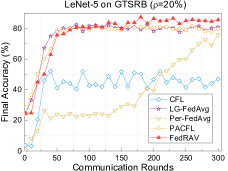
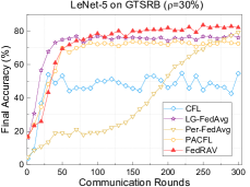
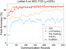
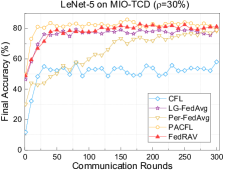
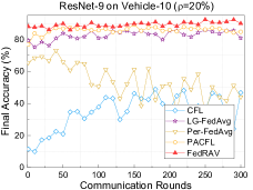
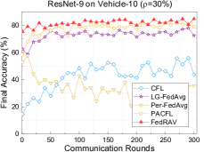
(a) GTSRB ($\rho=20\%$)             (b) GTSRB ($\rho=30\%$)              (c) MIO-TCD ($\rho=20\%$)          (d) MIO-TCD ($\rho=30\%$)              (e) Vehicle-10 ($\rho=20\%$)          (f) Vehicle-10 ($\rho=30\%$)

Figure 4: Comparison of different FL approaches.

V Experiments

V-A Experimental Setup

Datasets and Models. We consider traffic object classification task and evaluate our framework in three real-world datasets: GTSRB[12], MIO-TCD[13] and Vehicle-10, which are widely used to evaluate autonomous driving algorithms. GTSRB, the German traffic sign recognition benchmark, consists of 39270 images of 43 different traffic signs. The classification section of MIO-TCD contains a total of 52801 images from 11 categories of traffic participants. In this work, we also collected 36006 vehicle images from the Internet and divided them into ten categories, which we called Vehicle-10. For all experiments, we consider LetNet-5[14] for the GTSRB and MIO-TCD datasets, and ResNet-9[15] for the Vehicle-10.

Compared Baselines. First, we evaluate the effectiveness of our FedRAV framework. Then, we compare and evaluate the following single-model algorithms: FedAvg [1], FedProx [6], and FedNova [7]. In addition, we also evaluate several multi-model approaches: CFL [3], LG-FedAvg [16], Per-FedAvg [2], and PACFL [4].

Implementation Details. In all experiments, we suppose that 100 AVs participate in learning tasks. Unfortunately, the above three datasets do not provide metadata of vehicle GPS. We randomly generate location coordinates of 100 AVs for each dataset, ensuring that vehicles in proximity have comparatively similar data distributions. Note that this synthetic coordinate information of AV is only a supplement. In order to simulate the Non-IID label skewed setting, we randomly assign $\rho$ of the total labels of the dataset to each AV, i.e., $\rho=20\%$ or $\rho=30\%$. For all experiments, The number of training rounds is set to $T=300$, and $20\%$ of the AVs are sampled randomly to participate in the training process at each round. AV trains the local model by stochastic gradient descent with iteration $\kappa_{1}=10$ and batch-size $B=20$.

TABLE II: Quantitative comparison results across different datasets in ($\rho=20\%$ and $\rho=30\%$) Non-IID settings.

Dataset		GTSRB		MIO-TCD		Vehicle-10
Non-IID level $\rho$		$20\%$	$30\%$	$20\%$	$30\%$	$20\%$	$30\%$
Single-Model	FedAvg[1]	$84.98\pm 0.31$	$84.40\pm 1.87$	$63.93\pm 1.88$	$66.19\pm 0.94$	$62.18\pm 4.03$	$69.33\pm 6.04$
	FedProx[6]	$83.97\pm 0.95$	$\textbf{85.18}\pm\textbf{0.16}$	$64.25\pm 0.88$	$67.90\pm 1.04$	$56.03\pm 6.73$	$69.67\pm 6.83$
	FedNova[7]	$83.18\pm 1.05$	$85.13\pm 0.98$	$63.70\pm 3.66$	$67.57\pm 1.29$	$48.69\pm 8.47$	$68.65\pm 5.08$
Multi-Model	CFL[3]	$46.40\pm 1.34$	$53.34\pm 1.24$	$57.16\pm 0.95$	$52.83\pm 4.50$	$46.27\pm 1.01$	$44.92\pm 1.51$
	LG-FedAvg[16]	$80.55\pm 0.69$	$74.67\pm 1.20$	$86.42\pm 0.92$	$77.96\pm 1.63$	$81.69\pm 1.67$	$74.66\pm 1.84$
	Per-FedAvg[2]	$73.04\pm 4.82$	$78.23\pm 0.94$	$79.71\pm 1.81$	$77.89\pm 0.90$	$43.58\pm 13.2$	$31.78\pm 4.61$
	PACFL[4]	$79.31\pm 0.49$	$71.44\pm 0.94$	$88.44\pm 1.03$	$81.08\pm 1.90$	$86.43\pm 1.80$	$78.11\pm 0.85$
	FedRAV	$\textbf{86.55}\pm\textbf{0.83}$	$83.37\pm 1.21$	$\textbf{88.72}\pm\textbf{0.99}$	$\textbf{81.65}\pm\textbf{0.49}$	$\textbf{89.77}\pm\textbf{0.64}$	$\textbf{84.02}\pm\textbf{0.67}$

Evaluation Metrics. For single-model approaches, we evaluate the global model on the test set and report classification accuracy as experiment results. For multi-model approaches, each client holds a local test set in our experimental setting. We evaluate the personalized vehicular model on the local test set and use the average of final local test accuracy (a.k.a. final accuracy) to measure the performance of FL approaches.

V-B Performance Evaluation

As shown in Fig. 4, we observe that the FedRAV achieves the superior performance and outperforms the strong competitors on the most datasets with $K=5$, $\kappa_{1}=10$, $\kappa_{2}=10$, and $\gamma=0.5$. Besides, the CFL achieves the worst convergence on GTSRB and MIO-TCD datasets compared to other baselines, which owes to its failed clustering strategy. For example, CFL may partition a single AV into a separate cluster, leading to inadequate training. However, FedRAV can resolve this situation by gathering nearby AVs into a trainable region. In addition, Per-FedAvg converges with lower accuracy than other frameworks on the Vehicle-10 dataset. This is interpreted as highly Non-IID data that makes the approach suffer the suboptimal solution, i.e., optimization direction gradually deviates from the optimal solution. The accuracy curve illustrates that FedRAV can converge with similar accuracy as LG-FedAvg and PACFL before $100$ communication rounds. Henceforth, FedRAV achieves higher accuracy, whereas LG-FedAvg and PACFL converge at a lower accuracy. Therefore, FedRAV achieves comparable convergence and superior accuracy in Non-IID setting and does not induce more communication rounds in federated learning systems.

Table II presents the final accuracy over all baselines on three datasets. We find that most multi-model methods (LG-FedAvg, PACFL, and ours FedRAV) outperform the single-model methods on highly heterogeneous MIO-TCD and Vehicle-10 datasets, which further confirms the claim that the single model failed to fit heterogeneous client’s model parameter spaces. For the GTSRB dataset, single-model approaches converge the comparable accuracy with multi-model approaches. This is because the GTSRB dataset has weaker heterogeneity than the MIO-TCD and Vehicle-10. In particular, FedProx is slightly ahead of FedAvg on most datasets. FedRAV achieves superior performance and outperforms most of the state-of-the-art methods. Concretely, FedRAV improves final accuracy by $+6\%$ on GTSRB, $+2.3\%$ on MIO-TCD and $+8.08\%$ on Vehicle-10 for LG-FedAvg in $\rho=20\%$ setting, and enhances final accuracy by $+8.7\%$ on GTSRB, $+3.69\%$ on MIO-TCD and $+9.36\%$ on Vehicle-10 for LG-FedAvg in $\rho=30\%$ setting.

VI Conclusion

In this work, we propose a two-stage framework for learning personalized driving models from the scattered data collected from vehicles in various regions. It contains an efficient partitioning mechanism with one-shot communication for dividing large areas into sub-regions, and a FedRAV framework to employ the hypernetworks to learn personalized driving models against the heterogeneity, facilitating knowledge transfer among clients and regions. Finally, the extensive evaluations are conducted to verify the method’s effectiveness and superior performance compared to state-of-the-art methods.

References

- [1] B. McMahan, E. Moore, D. Ramage, S. Hampson, and B. A. y Arcas, “Communication-efficient learning of deep networks from decentralized data,” in Artificial intelligence and statistics. PMLR, 2017, pp. 1273–1282.
- [2] A. Fallah, A. Mokhtari, and A. Ozdaglar, “Personalized federated learning: A meta-learning approach,” arXiv preprint arXiv:2002.07948, 2020.
- [3] F. Sattler, K.-R. Müller, and W. Samek, “Clustered federated learning: Model-agnostic distributed multitask optimization under privacy constraints,” IEEE transactions on neural networks and learning systems, vol. 32, no. 8, pp. 3710–3722, 2020.
- [4] S. Vahidian, M. Morafah, W. Wang, V. Kungurtsev, C. Chen, M. Shah, and B. Lin, “Efficient distribution similarity identification in clustered federated learning via principal angles between client data subspaces,” in Proceedings of the AAAI Conference on Artificial Intelligence, vol. 37, no. 8, 2023, pp. 10 043–10 052.
- [5] Y. Zhao, M. Li, L. Lai, N. Suda, D. Civin, and V. Chandra, “Federated learning with non-iid data,” arXiv preprint arXiv:1806.00582, 2018.
- [6] T. Li, A. K. Sahu, M. Zaheer, M. Sanjabi, A. Talwalkar, and V. Smith, “Federated optimization in heterogeneous networks,” Proceedings of Machine learning and systems, vol. 2, pp. 429–450, 2020.
- [7] J. Wang, Q. Liu, H. Liang, G. Joshi, and H. V. Poor, “Tackling the objective inconsistency problem in heterogeneous federated optimization,” Advances in neural information processing systems, vol. 33, pp. 7611–7623, 2020.
- [8] M. Cordts, M. Omran, S. Ramos, T. Rehfeld, M. Enzweiler, R. Benenson, U. Franke, S. Roth, and B. Schiele, “The cityscapes dataset for semantic urban scene understanding,” in Proceedings of the IEEE conference on computer vision and pattern recognition, 2016, pp. 3213–3223.
- [9] S. Lloyd, “Least squares quantization in pcm,” IEEE transactions on information theory, vol. 28, no. 2, pp. 129–137, 1982.
- [10] D. Arthur and S. Vassilvitskii, “K-means++ the advantages of careful seeding,” in Proceedings of the eighteenth annual ACM-SIAM symposium on Discrete algorithms, 2007, pp. 1027–1035.
- [11] A. Shamsian, A. Navon, E. Fetaya, and G. Chechik, “Personalized federated learning using hypernetworks,” in International Conference on Machine Learning. PMLR, 2021, pp. 9489–9502.
- [12] S. Houben, J. Stallkamp, J. Salmen, M. Schlipsing, and C. Igel, “Detection of traffic signs in real-world images: The German Traffic Sign Detection Benchmark,” in International Joint Conference on Neural Networks, no. 1288, 2013.
- [13] Z. Luo, F. Branchaud-Charron, C. Lemaire, J. Konrad, S. Li, A. Mishra, A. Achkar, J. Eichel, and P.-M. Jodoin, “Mio-tcd: A new benchmark dataset for vehicle classification and localization,” IEEE Transactions on Image Processing, vol. 27, no. 10, pp. 5129–5141, 2018.
- [14] Y. LeCun, B. Boser, J. S. Denker, D. Henderson, R. E. Howard, W. Hubbard, and L. D. Jackel, “Backpropagation applied to handwritten zip code recognition,” Neural computation, vol. 1, no. 4, pp. 541–551, 1989.
- [15] K. He, X. Zhang, S. Ren, and J. Sun, “Deep residual learning for image recognition,” in Proceedings of the IEEE conference on computer vision and pattern recognition, 2016, pp. 770–778.
- [16] P. P. Liang, T. Liu, L. Ziyin, N. B. Allen, R. P. Auerbach, D. Brent, R. Salakhutdinov, and L.-P. Morency, “Think locally, act globally: Federated learning with local and global representations,” arXiv preprint arXiv:2001.01523, 2020.