Ground-state phase transitions in spin-1 Bose-Einstein condensates with spin-orbit coupling
Abstract
We investigate phase transitions of the ground state (GS) of spin-1 Bose-Einstein condensates under the combined action of the spin-orbit coupling (SOC) and gradient magnetic field. Introducing appropariate raising and lowering operators, we exactly solve the linear system. Analyzing the obtained energy spectrum, we conclude that simultaneous variation of the magnetic-field gradient and SOC strength leads to the transition of excited states into the GS. As a result, any excited state can transition to the GS, at appropriate values of the system’s parameters. The nonlinear system is solved numerically, showing that the GS phase transition, similar to the one in the linear system, still exists under the action of the repulsive nonlinearity. In the case of weak attraction, a mixed state appears near the GS transition point, while the GS transitions into an edge state under the action of strong attractive interaction.
I Introduction
Atomic Bose-Einstein condensates (BECs), thanks to their excellent experimental controllability, serve as versatile platforms for simulating and exploring various phenomena which were previously known in much more complex form in condensed-matter physics RepProgPhys.75.082401 ; Lewenstein . In particular, a great deal of interest was drawn to the BEC-enabled emulation of spin-orbit coupling (SOC), i.e., the effect of the electron spin on its motion in semiconductors. The original SOC plays a critical role in numerous quantum phenomena and applications, such as spin Hall effects RevModPhys.82.1959 , topological insulators RevModPhys.82.3045 , and the design of spintronic devices RevModPhys.76.323 , and more liu2020holding ; zhang2017spin ; han2018chiral ; lin2019effects ; zhang2019ground ; deng2012spin ; Liu2022Spin ; Li2013Double ; Zhu2022Vortex ; Zhu2022Main ; lu2015spin ; PRA_78_023616 ; FOP_Lu ; FOP_YYY ; FOP_YZHANG ; FOP_ZRX ; BEC-SOC GP eqns . In the past decade, one- nature09887 , two- Science.354.83 ; huang2016experimental , and three-dimensional Juzeliunas ; Science.372.271 synthetic SOC in binary atomic gases have been predicted and realized in experiments, providing pristine platforms for the observation of novel topological phenomena. The interplay between the synthetic SOC and intrinsic nonlinearity of ultracold atoms gives rise to a rich variety of matter-wave states, charactized by their topological properties and dynamical stability. These include plane waves Han Pu , vortices Kawakami ; Drummond ; Sakaguchi ; PhysRevE.89.032920 ; PhysRevE.94.032202 ; CNSNS ; xu2023vortex ; deng2024semi ; chen2020non ; guo2024stable , diverse species of solitons PhysRevLett.110.264101 ; 1D sol 2 ; 1D sol 3 ; 1D sol 4 ; Cardoso ; Lobanov ; 2D SOC gap sol Raymond ; SOC 2D gap sol Hidetsugu ; low-dim SOC ; yang2021matter ; liu2024osci ; wang2024bright ; li2023soliton ; kartashov2017solitons ; saka2022one ; karta2020stable , and skyrmions PhysRevLett.109.015301 ; dong2022vortex ; Skyrmion_ZYB ; Skyrmion_LCF . The experimental and theoretical achievements in this field are summarized in several reviews Spielman ; Galitski ; Ohberg ; Zhai ; SOC-sol-review ; tu2023ryd ; stepa2024spin ; zhang2023anha ; lyu2024super ; wang2022ground ; zhang2022farady ; li2022quantum ; xu2022three ; gangwar2022dynamics ; zhang2022spin ; zhang2023spin ; li2023bound ; CSF_YZJ .
The identification of the ground state (GS) in any setup, including BEC systems, is a problem of fundamental significance. In particular, an especially interesting possibility is to construct physically relevant systems which exhibit GS phase transitions, transforming original excited states into the GS as a result of variation of system’s parameters. In terms of the corresponding energy spectrum, the gap between the GS and the first excited state closes at the phase transition point. In this vein, it has been recently shown that in one- PhysRevA.106.063311 and two-dimensional PhysRevA.109.013326 two-component SOC BEC systems (in other words, in the SOC systems with spin 1/2) excited states with arbitrarily high quantum numbers can be transform into the GS by adjusting the SOC strength and the gradient magnetic field applied to the setup. Extending that work, we here aim to reveal a possibility of GS phase transitions in spin-1 (three-component) SOC BECs. It is natural to expect that, in comparison to their spin-1/2 counterparts, spin-1 systems exhibit more diverse properties Ma-Jia ; Adhikari ; He2022Multi ; Wang2023Non ; Lin2021Spin ; FOP_Song ; spin_1_PLA_QZHU ; spin_1_PRA_Gangwar ; spin_1_NJP_ZYP ; spin_1_PRA_Rajat ; spin_1_PRA_ZLC ; spin_1_PRA_LLU ; spin_1_PLA_JWANG . In particular, in the presence of repulsive and attractive spin-spin interactions, the GSs of the spin-1 systems are polar and ferromagnetic states ho , respectively.
In this work, we introduce a spin-1 SOC system which includes a gradient magnetic field and the harmonic-oscillator trapping potential. The linear version of the system with equal SOC strength and magnetic field gradient is solved exactly. Analysis of the respective energy spectrum reveals that simultaneously increase of these equal parameters reduces the system’s energy, so that higher energy levels feature larger reduction rates. Therefore, for suitable parameters, the system can undergo a GS phase transition, with any excited state being capable to transition into the GS. The full nonlinear system, including repulsive or attractive spin-spin interactions, is solved numerically. The solutions are mixed states, in the sense that they are built, essentially, as a superposition of several eigenstates of the linear system. In the case of relatively strong spin-spin attraction, the nonlinear system produces narrow (self-focused) edge states, so called because they spontaneously shift from the central position to an edge. This finding is explained by an analytical consideration. We analyze the results for the nonlinear system by monitoring magnetization of the eigensates.
The following presentation is structured as follows. The model is introduced in Section II. The exact linear solution is reported in Section III. Numerical solutions of the nonlinear system with repulsive and attractive interactions are produced in Sections. IV and V, respectively. The impact of the quadratic Zeeman effect on the system is discussed in Section VI. Finally, the paper is concluded by Section VII.
II The model
We consider an effectively one-dimensional spin-1 (three-component) 87Rb BEC under the action of SOC, the trapping harmonic potential, which is written in the scaled form as , and magnetic field
| (1) |
with constant gradient along the direction, while its -component is the bias factor, normalized to be . The form of SOC is chosen as that realized in the experiment nature09887 , i.e., , which corresponds to an equal-weight mixing of Rashba and Dresselhaus couplings. Here is the SOC strength, and the momentum operators are adopted in the scaled form, , by setting the atomic mass and the Planck’s constant to unity, i.e., . The standard set of spin-1 matrices is defined as
| (2) | ||||
For another form of SOC, such as , one may replace magnetic field (1) by , to produce the same results as those reported here.
The single-particule Hamiltonian corresponding to what is said above is written as
| (3) |
In the mean-field approximation, dynamics of the spinor wave functions, of the many-body condensate is governed by the system of Gross-Pitaevskii equations, which are presented here in the scaled form:
| (4) |
where is the total atomic density, and the local spin is
| (5) |
Further, coefficients and in Eq. (4) are strengths of the density-density and spin-spin interactions, respectively. We consider the natural case when the former interaction is repulsive, thus fixing (unless we set while addressing the linear system in Section 3), while the spin-spin interaction may have either sign.
Stationary solutions of Eq. (4) with chemical potential are sought for in the usual form,
| (6) |
with stationary wave functions
| (7) |
satisfying the following equations:
| (8) |
where stands for the complex conjugate. The total energy of the system is
| (9) |
Below, we exactly solve the linear system (8) with . Then, the nonlinear system is solved numerically, for the repulsive and attractive interactions alike.
Equations (4) are written in the scaled form. In physical units, a relevant value of the harmonic trapping frequency is Hz. The number of atoms in the condensates may be , which is sufficient for the experimental observation of the predicted patterns in full detail. The characteristic length, time and energy are identified as m, ms, and J, where kg is the atomic mass of 87Rb. The strength of SOC, denoted by , where is the laser wavelength, can be adjusted across a wide range of values, depending on the specific configurations of the laser system BEC-SOC GP eqns . Thus, shorter wavelengths of the laser illumination makes effective SOC strength greater. For instance, Nd:YLF lasers typically emit light with at nm or nm laser , which correspond, respectively, to the SOC strength of and .
III The exact solution of the linear system
Our first objective is to produce an exact solution of the linear version of Eq. (8) with (the balance between the SOC and gradient magnetic field). This linear problem amounts to the form of with Hamiltonian
| (10) |
To solve the linear problem exactly, we introduce an auxiliary operator,
| (11) |
where the raising and lowering operators are defined as and . The corresponding basis of wave functions with are provided by eigenstates of the harmonic oscillator LL , viz.,
| (12) |
where are the Hermite polynomials. Operators and act on wave function (12) according to the standard relations,
| (13) |
Note that the auxiliary operator (11) commutes with the Hamiltonian, i.e., , implying that they share the same eigenfunctions. Solving the eigenvalue equation
| (14) |
we obtain the corresponding eigenvalues,
| (15) |
The respective eigenfunctions for are
| (16) |
where the normalization coefficient ,
| (17) |
secures the usual condition,
| (18) |
For , the normalized wave function is
| (19) |
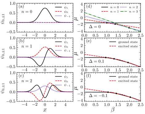
The quantum number in Eqs. (14) - (19) can be used to label the order of the eigenfunctions. Their typical profiles for are plotted in Figs. 1(a)-(c).
The eigenfunctions (16) and (19) are also eigenfunctions of the Hamiltonian , defined by Eq. (10) with the corresponding eigenvalues
| (20) |
It is seen that the SOC strength , which is equal to the magnetic-field gradient, in the case of the exact solution, alters the spectrum (20) of eigenvalues but does not affect the corresponding eigenfunctions (16). Figure 1(d) displays the dependence of on for the exact solution. Branches of with larger values of decrease more rapidly as functions of , which leads to intersections between the branches. The intersections between the ones corresponding to and , which carry, alternately, the minimum energies on two sides of the intersection points (i.e., the branches which represent the GS) directly imply the GS phase transitions. In other words, the combined effects of spin-orbit coupling and gradient magnetic field can close the gap between the ground state and first excited state, thereby inducing a GS phase transition. The corresponding critical points are obtained by solving equation :
| (21) |
Thus, by adjusting parameter , the states (16) with any quantum number can be transformed into the GS.
A basic principle of quantum mechanics is that, in the framework of the single Schrödinger equation, the GS cannot be degenerate LL . In the present case, the system of three coupled Schrödinger-like equations (8) violates this principle at critical points (21), as at these points two different eigenstates, corresponding to the intersecting branches , simultaneously represent the GS.
The analytical results were presented under the solvability condition . In the general case,
| (22) |
with offset between the magnetic field gradient and SOC strength , the linear system does not admit analytical solutions, but it can be solved approximately. To this end, solutions are looked for as finite combination of the harmonic-oscillator wave functions (12) truncated at :
| (23) |
where , and are coefficients to be determined. Here, we produce results for , which provides practically exact results. Substituting the ansatz based on Eqs. (22) and (23) in the linearization of Eq. (8), we obtain a set of coupled linear equations for , and :
| (24) |
Equations (24) can be solved by numerically by diagonalizion of the corresponding matrix. The corresponding GS phase transitions occur at intersection of the two lowest-energy branches, as shown in Figs. 1(e) and (f), which correspond to offsets and , respectively, in Eq. (22). The results clearly indicate that the GS phase transition occurs at , similar to what is found above in the exactly solvable linear system with .
IV Numerical results for the system with repulsive spin-spin interactions
Next, we address the spin-1 system in the full form, which is based on Eq. (4) including the nonlinear terms. To facilitate the comparison of nonlinear bound states with their linear counterparts, we here keep the same constraint which was imposed above to produce the exact solution of the linear system. In this case, the system’s GS can be found in a numerical form by means of the imaginary-time propagation method chiofalo ; Bao . In this context, we fix the total norm as , see Eq. (18). We used a -point grid to discretize the space, with ranging in the interval of . The spatial and time derivatives were handled by means of the Fourier transform and backward Euler scheme, respectively. The results definitely converged after steps.
We start the consideration of the nonlinear system with one featuring the repulsive spin-spin interaction, i.e., in Eq. (4). The term in the system’s energy accounting for the spin-spin interaction is
| (25) |
(recall is the total atomic density, and is the local spin defined as per Eq. (5)). To minimize the energy, local spins tend to evolve towards , which means the system will try to construct a polar state, with zero magnetization. Typical spinors corresponding to the polar states are
| (26) |
where , hence the local spin vector (5) is written as . In the polar state , particles are evenly distributed between the and components. In the polar state , all particles populate solely the component, hence the polar states always have .
In the general case, the magnetization vector of the spin-1 BEC is defined as wenlin
| (27) |
(recall is the matrix vector (2)), which obviously vanishes in the polar states. For linear solutions (16) and (19), takes values
| (28) |
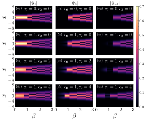
Figures 2 (), (),and () display maps of the distribution of absolute values of the three spinor components, in the numerically found GS for ranging from to , and . For the comparison’s sake, similar plots for the exact linear solution, with , are displayed in Figs. 2(). This is consistent with what is predicted by the exact linear solution (16). Note also that, with the increase of , the GS pattern develops a striped structure, which is a generic feature of SOC systems nature09887 ; stripe1 ; stripe2 . According to the linear solution (16), we can find that the wave functions of the three components are solutions of harmonic potential with adjacent quantum numbers. Due to the symmetry of the harmonic potential, the solutions alternate between odd and even parity as the quantum number increases. This leads to complementary properties between adjacent solutions, as shown in Figs. 2.
As the strength of the spin-spin repulsion increases, all critical points of the GS phase transition shift towards . This happens because, as mentioned above, the increase of drives all the system’s eigenstates closer to polar ones, hence a smaller difference between them needs a smaller SOC strength to perform the GS phase transition.
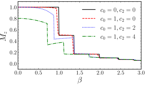
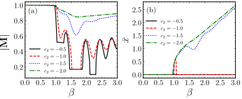
To produce a clear representation of the impact of the spin-spin interaction parameter on the GS magnetization , Fig. 3 depicts it as a function of for different fixed values of . It is seen that, in accordance with the above-mentioned trend of the suppression of the magnetization by the repulsive spin-spin interaction, decays with the increase of . Using Eq. (28), we obtain the decay rate of the magnetization with the increase of :
| (29) |
This result implies that, as increases, the decay of weakens, which is consistent with what is shown in Fig. 3.
The structure of the numerically found GS in can be analyzed if it represented by a superposition of the linear eigenstates (16),
| (30) |
where accounts for the weight of each eigenstate, satisfying the normalization condition, , which is a corollary of the unitary normalization adopted for . We used in our calculations, which efficiently provides sufficiently accurate results.
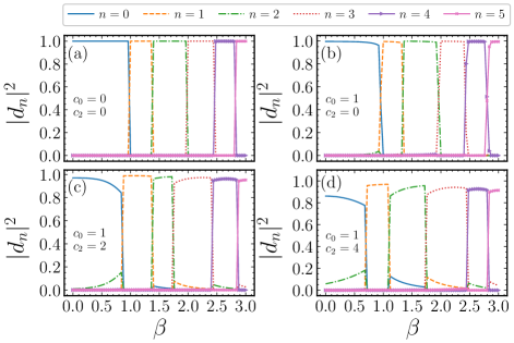
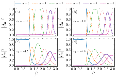
Figure 4 shows the dependence of weights on for (a) , (b) , (c) and (d) . Figure 4(a) corresponds to the linear solution, where the weights of the two eigenstates with adjacent quantum numbers, i.e., and , exhibit a discontinuous change at the GS phase transition point. For example, at the first phase transition point where , the weight decreases from 1 to 0, while the weight increases from 0 to 1. Figure 4(b) corresponds to , and we can see that the pattern is similar to the one in the linear system. As increases, Figs. 4(c) and (d) demonstrate that the system’s GS becomes a superposition of a pair of next-nearest-neighbor eigenstates, labeled by quantum number and . As previously mentioned, although the phase transition point has shifted closer to , it can still be easily identified in Fig. 4.
V Numerical results for the system with attractive spin-spin interactions
Next, we consider the nonlinear system with the attractive spin-spin attraction, i.e., in Eq. (4). Figure 5 displays maps of the distribution of absolute values of the three spinor components, in the numerically found GS for ranging from to , and , cf. Fig. 2. The figure exhibits completely different patterns for different values of . At and , we observe the presence of spatially symmetric GS, with , in Figs. 5() and (). For the stronger spin-spin attraction, viz., and , the GS take the form of spatially narrow edge states, strongly shifted to , at . The narrowness of the GS in this case is explained by the self-focusing effect of the attractive nonlinearity. The shift from the central position towards , which is explained analytically below, is possible, as Eq. (4) is not symmetric wih respect to the reflection, . The symmetry breaking is characterized by the dependence of on , as shown in Fig. 7(b), where is the average displacement.
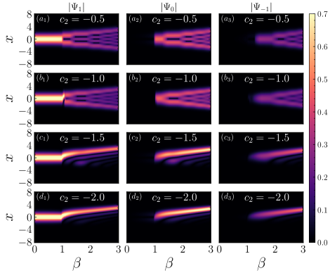
Figure 6 shows the dependence of weights on for and . First, it is clearly seen that, for , under the action of the spin-spin attraction (), the GS is virtually tantamount to the linear eigenstate with , the entire structure of the decomposition being nearly identical for and . Near the critical point of the linear system, mixed states emerge, which are chiefly formed as a superposion of eigenstates with quantum numbers and , with the weights satisfying . Far from the critical point, the GS reverts to a shape which is close to the respective linear eigenstate, as seen in Figs. 6(a) and (b). Thus, we conclude that, in the case of the weak spin-spin attraction, viz., for , the GS phase transition remains close to the one in the linear system, but between the mixed states, which are superpositions of states and . As the attractive interaction strengthens, viz., in the cases of and , the system’s GS becomes narrow edge (spatially shifted) states, which are, essentially, superpositions of several linear eigenstates, as seen in Figs. 6(c) and (d).
The mixed states, which are formed, approximately, by the superposition of two eigenstates, feature phase difference between the respective weights and (see Eq. (30)). Accordingly, one may consider as a real number, while . Then, the wave function of the mixed state is written as
| (31) |
where the eigenfunctions are defined in Eq. (16) and Eq. (19). The magnetization (27) corresponding to this wave function is
| (32) |
| (33) |
Note that, unlike the linear eigenstates, the -component of the magnetization of the mixed state does not vanish. It attains a maximum in the case when the two weights are equal, .
Figure 7(a) shows the dependence of the absolute value of the magnetization, , on for different values of the spin-spin-attraction coefficient . First, we find that, for the same , larger pushes closer to the limit value . For the mixed states corresponding to and , the curves include fragments downward-opening parabolas, which can be explained by the consideration of Eq. (32).
The formation of the edge (spatially-shifted) GS can be analyzed in terms of energy. To minimize the energy induced by spin-spin interactions, as given by Eq. (25) with , the local spin vector tends to have . Therefore, the respective GS tends to become a ferromagnetic state. Typical spinors corresponding to such states are
| (34) |
cf. expressions (26) for the polar states. The state corresponding to implies that all atoms are collected in the component, the same as in the linear solution (19) with . This is the reason why the spin-spin interaction does not affect states with quantum number at , as shown in Figs. 5 and 6.
The GS corresponding to spinor in Eq. (34), indicates that the wave functions of the three components are related by
| (35) |
In this case, the spin-orbit coupling and Zeeman splitting can be neglected because their energies,
| (36) | ||||
and
| (37) |
are vanishingly small. By substituting these approximations in Eq. (8), we reduce it to a single-component equation,
| (38) |
which features an effective potential . Thus the atoms tend to accommodate around the obvious minimum of the potential, , which is shifted off the central position, as seen in Figs. 5() and ().
VI The ground state of the system in the presence of the quadratic Zeeman shift
The above discussions focused only on the linear Zeeman effect; however, in actual experiments, the quadratic Zeeman shift can have a significant impact on the results. Incorporating the quadratic Zeeman effect, with strength , into Eq. (4) by introducing the respective Hamiltonian term , the modified Gross-Pitaevskii equation is written as wenlin ; QZ
| (39) |
where the magnetic field is the same as above, viz., . To eliminate the influence of spin-spin interactions on the system’s GS, we set in this section, while the density-density interaction is kept fixed at .
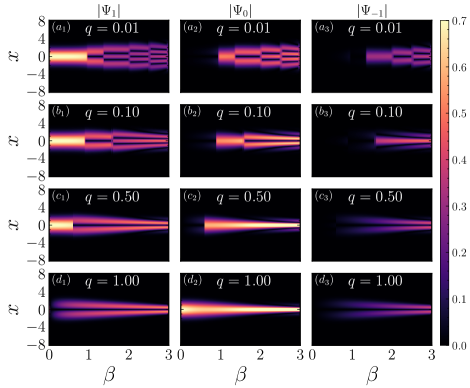
We employed the imaginary-time evolution method to produce the system’s GS for different values of . The numerical results are presented in Fig. 8. For small values of , such as , the GS phase transitions still occurs, being very similar to those reported above. However, as increases, specifically at , only a few lowest GS phase transitions take place. We also observe that, as increases, the range of the wave function distribution in the direction narrows.
For , the quadratic Zeeman effect is the dominant factor in the system. Thus, the distribution of the GS wave function can be determined by analyzing the energy induced by the quadratic Zeeman effect, with the energy expressed as
| (40) |
We further simplify Eq. (40) by introducing the unitary operator
| (41) |
where is the identity matrix of size . The physical meaning of this operator is the clockwise rotation by an angle around the -axis, which makes the magnetic field pointing in the direction. The rotation angle is determined by expressions
| (42) |
Till now, it is easy to check . With the aid of the unitary operator (41), the energy (40) can be simplified to:
| (43) |
It is evident that an effective potential emerges, which corresponds to the harmonic-oscillator one. As increases, the strength of the potential grows, leading to a narrowing of the wavefunction distribution along the -direction.
Being concerned with the GS of the system, we minimize energy . It is important to note that, when , the energy reaches its minimum, which is . Thus, we obtain the corresponding spinor
| (44) |
Next, we consider two essential spatial regions. The first one corresponds to , where we have and , obtaining and . The second region corresponds to , where and , resulting in and . These conclusions precisely explain the wavefunction distribution patterns observed in Figs. 8() and ()). In the former figure, the GS transition occurs at , and the pattern beyond this point is similar to the one in Fig. 8(). We conclude that the particles predominantly occupy component around , corresponding to . As gradually increases, the particles are transferred to components , until full occupancy is achieved, corresponding to the spinor .
VII Conclusion
This work is focused on the phase transition in the GS (ground state) in spin-1 BECs, considering the combined effects of SOC (spin-orbit coupling) and gradient magnetic fields. The linear system is solved exactly by means of the formulation using raising and lowering operators. Through the analysis of the energy spectrum, we have demonstrated that, following the variation of the magnetic-field gradient and SOC strength, the system undergoes a series of GS phase transitions, allowing all excited states to transition into the GS.
The nonlinear system, including the density-density and spin-spin interactions, has been solved numerically. In the case of the spin-spin repulsion, the results obtained for the nonlinear system are similar to their counterpart for the linear one. The results are drastically different in the case of the spin-spin attraction: the relatively weak interaction gives rise to bimodal mixed states near the GS phase-transition points of the linear system, while stronger interaction creates the narrow GS as the edge state shifted off the central position. The latter finding is explained by means of the analytical consideration. A natural continuation of the current work is to consider those problems in 2D, where we can explore the GS phase transitions of vortex states.
Acknowledgments
This work was supported by the GuangDong Basic and Applied Basic Research Foundation through grant No. 2023A1515110198, Natural Science Foundation of Guangdong Province through grants Nos. 2024A1515030131 and 2021A1515010214, Foundation for Distinguished Young Talents in Higher Education of Guangdong No. 2024KQNCX150, National Natural Science Foundation of China through grants Nos. 12274077, 62405054, 12475014 and 11905032, the Research Found of the Guangdong-Hong Kong-Macao Joint Laboratory for Intelligent Micro-Nano Optoelectronic Technology through grant No. 2020B1212030010, and Israel Science Foundation through Grant No. 1695/22.
References
- (1) P. Hauke, F. M. Cucchietti, L. Tagliacozzo, I. Deutsch, and M. Lewenstein, Can one trust quantum simulators? Rep. Prog. Phys. 75, 082401 (2012).
- (2) M. Lewenstein, A. Sanpera, and V. Ahufinger, Ultracold Atoms in Optical Lattices: Simulating Quantum Many-Body Systems (Oxford: Oxford University Press, 2012).
- (3) D. Xiao, M.-C. Chang, and Q. Niu, Berry phase effects on electronic properties, Rev. Mod. Phys. 82, 1959 (2010).
- (4) M. Z. Hasan and C. L. Kane, Colloquium: Topological insulators, Rev. Mod. Phys. 82, 3045 (2010).
- (5) I. Z̆utić, J. Fabian, and S. D. Sarma, Spintronics: Fundamentals and applications, Rev. Mod. Phys. 76, 323 (2004).
- (6) B. Liu, R. Zhong, Z. Chen, X. Qin, H. Zhong, Y. Li, and B. A. Malomed, Holding and transferring matter-wave solitons against gravity by spin-orbit-coupling tweezers, New J. Phys. 22, 043004 (2020).
- (7) X. F. Zhang, M. Kato, W. Han, S. G. Zhang, and H. Saito, Spin-orbit-coupled Bose-Einstein condensates held under a toroidal trap, Phys. Rev. A 95, 033620 (2017).
- (8) W. Han, X. F. Zhang, D. S. Wang, H. F. Jiang, W. Zhang, and S. G. Zhang, Chiral supersolid in spin-orbit-coupled Bose gases with soft-core long-range interactions, Phys. Rev. Lett. 121, 030404 (2018).
- (9) L. Wen, Y. Liang, J. Zhou, Y. Peng, L. Xia, L. B. Niu, and X. F. Zhang, Effects of linear Zeeman splitting on the dynamics of bright solitons in spin-orbit coupled Bose-Einstein condensates, Acta Phys. Sinica 68, 080301 (2019).
- (10) R. F. Zhang, Y. Zhang, and L. li, Ground states of spin-orbit-coupled Bose Einstein condensates in the presence of external magnetic field, Phys. Lett. A 383, 3175 (2019).
- (11) Y. Deng, J. Cheng, H. Jing, C. P. Sun, and S. Yi, Spin-orbit coupled dipolar Bose-Einstein condensates, Phys. Rev. Lett. 108, 125301 (2012).
- (12) K. Liu, H. He, C. Wang, Y. Chen, and Y. Zhang, Spin-orbit-coupled spin-1 Bose-Einstein condensates in a toroidal trap: Even-petal-number necklacelike state and persistent flow, Phys. Rev. A 105 013323 (2022).
- (13) Z. Li, J. Z. Wang, and L. B. Fu, Double Barrier Resonant Tunneling in Spin-Orbit Coupled Bose-Einstein Condensates, Chin. Phys. Lett. 30, 010301 (2013).
- (14) H. Zhu, S. G. Yin, and W. M. Liu, Vortex chains induced by anisotropic spin-orbit coupling and magnetic field in spin-2 Bose-Einstein condensates, Chin. Phys. B 31, 060305 (2022).
- (15) H. Zhu, S. G. Yin, and W. M. Liu, Manipulating vortices in F=2 Bose-Einstein condensates through magnetic field and spin-orbit coupling, Chin. Phys. B 31, 040306 (2022).
- (16) H. Lü, S. B. Zhu, J. Qian, and Y. Z. Wang, Spin-orbit coupled Bose-Einstein condensates with Rydberg-dressing interaction, Chin. Phys. B 24, 090308 (2015).
- (17) T. D. Stanescu, B. Anderson, and V. M. Galitski, Spin-orbit coupled Bose-Einstein condensates, Phys. Rev. A 78, 023616 (2008).
- (18) P. Lu, X. Zhang and C. Dai, Dynamics and formation of vortices collapsed from ring dark solitons in a two-dimensional spin-orbit coupled Bose-Einstein condensate, Front. Phys. 17, 42501 (2022).
- (19) Y. Yang, P. Gao, L. Zhao, and Zh. Yang, Kink-like breathers in Bose-Einstein condensates with helicoidal spin-orbit coupling,Front. Phys. 17, 32503 (2022).
- (20) Y. Zhang, M. E. Mossman, T. Busch, P. Engels, and C. Zhang, Properties of spin-orbit-coupled Bose-Einstein condensates, Front. Phys. 11, 118103 (2016).
- (21) R. X. Zhong, Z. P. Chen, C. Q. Huang, Z. H. Luo, H. S.Tan, B. A. Malomed, and Y. Y. Li, Self-trapping undertwo-dimensional spin-orbit coupling and spatially growing repulsive nonlinearity, Front. Phys. 13, 130311 (2018).
- (22) Y. Zhang, L. Mao, and C. Zhang, Mean-field dynamics of spin-orbit coupled Bose-Einstein condensates, Phys. Rev. Lett. 108, 035302 (2012).
- (23) Y.-J. Lin, K. Jiménez-García, and I. B. Spielman, Spin-orbit-coupled Bose-Einstein condensates, Nature (London)471, 83 (2011).
- (24) Z. Wu, L. Zhang, W. Sun, X.-T. Xu, B.-Z. Wang, S.-C. Ji, Y. Deng, S. Chen, X.-J. Liu, and J.-W. Pan, Realization of two-dimensional spin-orbit coupling for Bose-Einstein condensates, Science 354, 83 (2016).
- (25) L. Huang, Z. Meng, P. Wang, P. Peng, S. L. Zhang, L. Chen, D. Li, Q. Zhou, and J. Zhang, Experimental realization of two-dimensional synthetic spin-orbit coupling in ultracold Fermi gases, Nat. Phys. 12, 540 (2016).
- (26) B. M. Anderson, G. Juzeliūnas, V. M. Galitski, and I. B. Spieman, Synthetic 3D spin-orbit coupling, Phys. Rev. Lett. 108, 235301 (2012).
- (27) Z.-Y. Wang, X.-C. Cheng, B.-Z. Wang, J.-Y. Zhang, Y.-H. Lu, C.-R. Yi, S. Niu, Y. Deng, X.-J. Liu, S. Chen, and J.-W. Pan, Realization of an ideal Weyl semimetal band in a quantum gas with 3D spin-orbit coupling, Science 372, 271 (2021).
- (28) Y.-C. Zhang, Z.-W. Zhou, B. A. Malomed, and H. Pu, Stable solitons in three dimensional free space without the ground state: Self-trapped Bose-Einstein condensates with spin-orbit coupling, Phys. Rev. Lett. 115, 253902 (2015).
- (29) T. Kawakami, T. Mizushima and K. Machida, Textures of F=2 spinor Bose-Einstein condensates with spin-orbit coupling, Phys. Rev. A 84, 011607 (2011).
- (30) B. Ramachandhran, B. Opanchuk, X.-J. Liu, H. Pu, P. D. Drummond, and H. Hu, Half-quantum vortex state in a spin-orbit-coupled Bose-Einstein condensate, Phys. Rev. A85, 023606 (2012).
- (31) H. Sakaguchi, B. Li, and B. A. Malomed, Creation of two-dimensional composite solitons in spin-orbit-coupled self-attractive Bose-Einstein condensates in free space, Phys. Rev. E89, 032920 (2014).
- (32) H. Sakaguchi, E. Y. Sherman, and B. A. Malomed, Vortex solitons in two-dimensional spin-orbit coupled Bose-Einstein condensates: Effects of the Rashba-Dresselhaus coupling and Zeeman splitting, Phys. Rev. E94, 032202 (2016).
- (33) H. Sakaguchi and B. Li, Vortex lattice solutions to the Gross-Pitaevskii equation with spin-orbit coupling in optical lattices, Phys. Rev. A87, 015602 (2013).
- (34) H.-B. Luo, B. A. Malomed, W.-M. Liu, and L. Li, Bessel vortices in spin-orbit-coupled binary Bose-Einstein condensates with Zeeman splitting, Communications in Nonlinear Science and Numerical Simulation, 115, 106769 (2022).
- (35) X. Xu, F. Zhao, Y. Zhou, B. Liu, X. Jiang, B. A. Malomed, Y. Li, Vortex gap solitons in spin-orbit coupled Bose-Einstein condensates with competing nonlinearities, Communications in Nonlinear Science and Numerical Simulation 117, 106930 (2023).
- (36) X. Chen, Z. Deng, X. Xu, S. Li, Z. Fan, Z. Chen, B. Liu, Y. Li, Nonlinear modes in spatially confined spin-orbit-coupled Bose-Einstein condensates with repulsive nonlinearity, Nonlinear Dyn. 101, 569 (2020).
- (37) H. Deng, Ji. L, Zh. Chen, Y. Liu, D. Liu, Ch. Jiang, Ch. Kong, and B. A. Malomed, Semi-vortex solitons and their excited states in spin-orbit-coupled binary bosonic condensates, Phys. Rev. E 109, 064201 (2024).
- (38) Y. Guo, M. Idrees, J. Lin and H. Li, Stable stripe and vortex solitons in two dimensional spin-orbit coupled Bose-Einstein condensates, Commun. Theor. Phys. 76, 065003 (2024).
- (39) V. Achilleos, D. J. Frantzeskakis, P. G. Kevrekidis, and D. E. Pelinovsky, Matter-Wave Bright Solitons in Spin-Orbit Coupled Bose-Einstein Condensates, Phys. Rev. Lett. 110, 264101 (2013).
- (40) Y. Xu, Y. Zhang, and B. Wu, Bright solitons in spin-orbit-coupled Bose-Einstein condensates, Phys. Rev. A87, 013614 (2013).
- (41) L. Salasnich and B. A. Malomed, Localized modes in dense repulsive and attractive Bose-Einstein condensates with spin-orbit and Rabi couplings, Phys. Rev. A87, 063625 (2013).
- (42) Y. V. Kartashov, V. V. Konotop, and F. Kh. Abdullaev, Gap Solitons in a Spin-Orbit-Coupled Bose-Einstein Condensate, Phys. Rev. Lett. 111, 060402 (2013).
- (43) L. Salasnich, W. B. Cardoso, and B. A. Malomed, Localized modes in quasi-two-dimensional Bose-Einstein condensates with spin-orbit and Rabi couplings, Phys. Rev. A90, 033629 (2014).
- (44) V. E. Lobanov, Y. V. Kartashov, and V. V. Konotop, Fundamental, Multipole, and Half-Vortex Gap Solitons in Spin-Orbit Coupled Bose-Einstein Condensates, Phys. Rev. Lett. 112, 180403 (2014).
- (45) Y. Li, Y. Liu, Z. Fan, W. Pang, S. Fu, and B. A. Malomed, Two-dimensional dipolar gap solitons in free space with spin-orbit coupling, Phys. Rev. A95, 063613 (2017).
- (46) H. Sakaguchi and B. A, Malomed, One- and two-dimensional gap solitons in spin-orbit-coupled systems with Zeeman splitting, Phys. Rev. A97, 013607 (2018).
- (47) Y. V. Kartashov, L. Torner, M. Modugno, E. Ya. Sherman, B. A. Malomed, and V. V. Konotop, Multidimensional hybrid Bose-Einstein condensates stabilized by lower-dimensional spin-orbit coupling, Phys. Rev. Research 2, 013036 (2020).
- (48) Y. Yang, P. Gao, Z. Wu, L. C. Zhao, and Z. Y. Yang, Matter-wave stripe solitons induced by helicoidal spin-orbit coupling, Ann. Phys. 431, 168562 (2021).
- (49) F. Liu, H. Triki, Q. Zhou, Oscillatory nondegenerate solitons in spin-orbit coupled spin-1/2 Bose-Einstein condensates with weak Raman coupling, Chaos, Solitons and Fractals 186, 115257 (2024).
- (50) Q. Wang, J. Qin, J. Zhao, L. Qin, Y. Zhang, X. Feng, L. Zhou, Ch. Yang, Y. Zhou, Z. Zhu, W. Liu, and X. Zhao, Bright solitons in a spin-orbit-coupled dipolar Bose-Einstein condensate trapped within a double-lattice, Opt. Express 32, 6658 (2024).
- (51) X. Li, J. Qi, D. Zhao, W. Liu, Soliton solutions of the spin-orbit coupled binary Bose-Einstein condensate system. Acta Phys. Sin., 72, 106701 (2023).
- (52) Y. V. Kartashov and V. V. Konotop, Solitons in Bose-Einstein condensates with helicoidal spin-orbit coupling, Phys. Rev. Lett. 118, 190401 (2017).
- (53) H. Sakaguchi and B. A. Malomed, One- and two-dimensional solitons in spin-orbit-coupled Bose-Einstein condensates with fractional kinetic energy, J. Phys. B: At. Mol. Opt. Phys. 55, 155301 (2022).
- (54) Y. V. Kartashov, E. Y. Sherman, B. A. Malomed, and V.V. Konotop, Stable two-dimensional soliton complexes in Bose-Einstein condensates with helicoidal spin-orbit coupling, New J. Phys. 22, 103014 (2020)
- (55) T. Kawakami, T. Mizushima, M. Nitta, and K. Machida, Stable Skyrmions in SU(2) Gauged Bose-Einstein Condensates, Phys. Rev. Lett. 109, 015301 (2012).
- (56) B. Dong, S. Chen, X. Zhang, Vortex, stripe, Skyrmion lattice, and localized states in a spin-orbit coupled dipolar condensate, Annals of Physics 447, 169140 (2022).
- (57) G. Chen, T. Li, and Y. Zhang, Symmetry-protected skyrmions in three-dimensional spin-orbit-coupled Bose gases, Phys. Rev. A 91, 053624 (2015).
- (58) C. Liu and W. M. Liu, Spin-orbit-coupling-induced half-skyrmion excitations in rotating and rapidly quenched spin-1 Bose-Einstein condensates, Phys. Rev. A 86, 033602 (2012).
- (59) I. B. Spielman, Light induced gauge fields for ultracold neutral atoms, Annual Rev. Cold At. Mol. 1, 145 (2012).
- (60) P. Tu, Q. Wang, K. Shao, Y. Zhao, J. Ma, R. Su, and Y. Shi, Rydberg-dressed Bose-Einstein condensate with spin-orbit coupling confined in a radially periodic potential, J. Phys. B: At. Mol. Opt. Phys. 56, 15LT01 (2023).
- (61) V. A. Stephanovich, E. V. Kirichenko, G. Engel, and A. Sinner, Spin-orbit-coupled fractional oscillators and trapped Bose-Einstein condensates, Phys. Rev. E 109, 014222 (2024).
- (62) K. Zhang and Y. Chen, Anharmonicity-induced phase transition of spin-orbit coupled Bose-Einstein condensates, J. Phys. B: At. Mol. Opt. Phys. 56, 025303 (2023).
- (63) H. Lyu, Y. Chen, Q. Zhu, and Y. Zhang, Supercurrent-carrying supersolid in spin-orbit-coupled Bose-Einstein condensates, Phys. Rev. Research 6, 023048 (2024).
- (64) J. Wang, Y. Li, S. Yang, Ground-state phase diagrams in spin-orbit coupled spin-3 Bose-Einstein condensates, Physica A 597, 127244 (2022).
- (65) H. Zhang, Sh. Liu, and Y. Zhang, Faraday patterns in spin-orbit-coupled Bose-Einstein condensates, Phys. Rev. A 105, 063319 (2022).
- (66) J. Li , E. Ya Sherman, and A. Ruschhaupt, Quantum heat engine based on a spin-orbit- and Zeeman-coupled Bose-Einstein condensate, Phys. Rev. A 106, L030201 (2022).
- (67) S. Xu, Y. Lei, J. Du, Y. Zhao, R. Hua, J. Zeng, Three-dimensional quantum droplets in spin-orbit-coupled Bose-Einstein condensates, Chaos, Solitons and Fractals 164, 112665 (2022).
- (68) S. Gangwar, R. Ravisankar, P. Muruganandam, and P. Mishra, Dynamics of quantum solitons in Lee-Huang-Yang spin-orbit-coupled Bose-Einstein condensates, Phys. Rev. A 106, 063315 (2022).
- (69) X. Zhang, L. Wen, L. Wang, G.-P. Chen, R.-B. Tan, and H. Saito, Spin-orbit-coupled Bose gases with nonlocal Rydberg interactionsheld under a toroidal trap, Phys. Rev. A 105, 033306 (2022).
- (70) X. Zhang, L. Xu, S. Yang, Spin-density separation of spin-orbit coupled Bose-Einstein condensates under rotation, Phys. Lett. A, 487, 129128 (2023).
- (71) Ch. Li, V. V. Konotop, B. A. Malomed, Y. V. Kartashov, Bound states in Bose-Einstein condensates with radially-periodic spin-orbit coupling, Chaos, Solitons and Fractals 174, 113848 (2023).
- (72) V. Galitski and I. B. Spielman, Spin-orbit coupling in quantum gases, Nature (London)494, 49-54 (2013).
- (73) N. Goldman, G. Juzeliūnas, P. Öhberg, and I. B. Spielman, Light-induced gauge fields for ultracold atoms, Rep. Prog. Phys. 77, 126401 (2014).
- (74) B. A. Malomed, Creating solitons by means of spin-orbit coupling, EPL 122, 36001 (2018).
- (75) H. Zhai, Degenerate quantum gases with spin-orbit coupling: a review, Rep. Prog. Phys. 78, 026001 (2015).
- (76) Z. Ye, Y. Chen, Y. Zheng, X. Chen, B. Liu, Symmetry breaking of a matter-wave soliton in a double-well potential formed by spatially confined spin-orbit coupling, Chaos, Solitons and Fractals 130, 109418 (2020).
- (77) H.-B. Luo, B. A. Malomed, W.-M. Liu, and L. Li, Tunable energy-level inversion in spin-orbit-coupled Bose-Einstein condensates, Phys. Rev. A106, 063311 (2022).
- (78) H.-B. Luo, L. Li, B. A. Malomed, Y. Li, and B. Liu, Energy-level inversion for vortex states in spin-orbit-coupled Bose-Einstein condensates, Phys. Rev. A109, 013326 (2024).
- (79) D. Ma and C. Jia, Soliton oscillation driven by spin-orbit coupling in spinor condensates, Phys. Rev. A 100, 023629 (2019).
- (80) S. K. Adhikari, Phase separation of vector solitons in spin-orbit-coupled spin-1 condensates, Phys, Rev. A 100, 063618 (2019).
- (81) J. T. He, P. P. Fang, and J. Lin, Multi-type solitons in spin-orbit coupled spin-1 Bose-Einstein condensates, Chin. Phys. Lett. 39, 020301 (2022).
- (82) J. Wang, J. C. Liang, Z. F. Yu, A. Q. Zhang, and A. X. Zhang, Nonlinear modes coupling of trapped spin-orbit coupled spin-1 Bose-Einstein condensates, Chin. Phys. B 32, 090305 (2023).
- (83) J. Lin, T. He, J. Bai, B. Liu, and H. Y. Wang, Spin-orbit-coupled spin-1 Bose-Einstein condensates confined in radially periodic potential, Chin. Phys. B 30, 030302 (2021).
- (84) S. W. Song, L. Wen, C. F. Liu, S. C. Gou, and W. M. Liu, Ground states, solitons and spin textures in spin-1 Bose-Einstein condensates, Front. Phys. 8, 302 (2013).
- (85) Q. Zhu, L. Pan, Dynamical excitation of spin-orbit coupled spin-1 Bose-Einstein condensate in a narrow box trap, Phys. Lett. A 481, 129005 (2023).
- (86) J. Wang, J. Liang, Z. Yu, A. Zhang, A. Zhang, J. Xue, Magnetized and unmagnetized phases of trapped spin-orbit coupled spin-1 Bose-Einstein condensates, Phys. Lett. A 471, 128801 (2023).
- (87) S. Gangwar, R. Ravisankar, H. Fabrelli, P. Muruganandam, and P. Mishra, Emergence of unstable avoided crossing in the collective excitationsof spin-1 spin-orbit-coupled Bose-Einstein condensates, Phys. Rev. A 109, 043306 (2024).
- (88) Y. Chen, H. Lyu, Y. Xu and Y. Zhang, Elementary excitations in a spin-orbit-coupled spin-1 Bose-Einstein condensate, New J. Phys. 24, 073041 (2022).
- (89) Rajat, A. Roy, and S. Gautam, Collective excitations in cigar-shaped spin-orbit-coupled spin-1 Bose-Einstein condensates, Phys. Rev. A 106, 013304 (2022).
- (90) L. C. Zhao, X. W. Luo, and C. Zhang, Magnetic stripe soliton and localized stripe wave in spin-1 Bose-Einstein condensates, Phys. Rev. A 101, 023621 (2020).
- (91) J. Li, H. Luo, and L. Li, Bessel vortices in spin-orbit-coupled spin-1 Bose-Einstein condensates, Phys. Rev. A 106, 063321 (2022).
- (92) H. Zhao, K.-Y. Li, S.-B. Dai, Z.-H. Tu, Q.-G. Yang, S.-Q. Zhu, H. Yin, Z. Li, and Z.-Q. Chen, Nanosecond pulsed deep-red laser source by intracavity frequency-doubled crystalline Raman laser, Optics Letters 46, 13 (2021).
- (93) T.-L. Ho, Spinor Bose Condensates in Optical Traps, Phys. Rev. Lett. 81, 4 (1998).
- (94) L. D. Landau and E. M. Lifshitz, Quantum Mechanics: Nonrelativistic Theory (Nauka Publishers, Moscow, 1974).
- (95) M. L. Chiofalo, S. Succi, and M. P. Tosi, Ground state of trapped interacting Bose-Einstein condensates by an explicit imaginary-time algorithm, Phys. Rev. E 62, 7438-7444 (2000).
- (96) W. Z. Bao and Q. Du, Computing the ground state solution of Bose-Einstein condensates by a normalized gradient flow, SIAM J. Sci. Comp. 25, 1674-1697 (2004).
- (97) Y. Li, L. P. Pitaevskii, and S. Stringari, Quantum Tricriticality and Phase Transitions in Spin-Orbit Coupled Bose-Einstein Condensates, Phys. Rev. Lett. 108, 225301 (2012).
- (98) C. Wang, C. Gao, C.-M. Jian, and H. Zhai, Spin-Orbit Coupled Spinor Bose-Einstein Condensates, Phys. Rev. Lett. 105, 225301 (160403).
- (99) L. Wen, Q. Sun, H. Q. Wang, A. C. Ji, and W. M. Liu, Ground state of spin-1 Bose-Einstein condensates with spin-orbit coupling in a Zeeman field, Phys. Rev. A86, 043602 (2012).
- (100) J. Stenger, S. Inouye, D. M. Stamper-Kurn, H.-J. Miesner, A. P. Chikkatur and W. Ketterle, Spin domains in ground-state Bose-Einstein condensates, Nature (London)396, 345-348 (1998).