Analytical Formula for Fractional-Order Conditional Moments of Nonlinear Drift CEV Process with Regime Switching: Hybrid Approach with Applications
Division of Computational Science
Faculty of Science, Prince of Songkla University
Songkhla 90110, Thailand
kittisak.ch@psu.ac.th
&
Department of Mathematics and Computer Science
Faculty of Science, Chulalongkorn University
Bangkok 10330, Thailand
khamron.m@chula.ac.th
&
Department of Mathematics and Computer Science
Faculty of Science, Chulalongkorn University
Bangkok 10330, Thailand
6373011023@student.chula.ac.th
&
Department of Mathematics
Faculty of Science, Kasetsart University
Bangkok 10900, Thailand
phiraphat.sut@ku.th
Abstract
This paper introduces an analytical formula for the fractional-order conditional moments of nonlinear drift constant elasticity of variance (NLD-CEV) processes under regime switching, governed by continuous-time finite-state irreducible Markov chains. By employing a hybrid system approach, we derive exact closed-form expressions for these moments across arbitrary fractional orders and regime states, thereby enhancing the analytical tractability of NLD-CEV models under stochastic regimes. Our methodology hinges on formulating and solving a complex system of interconnected partial differential equations derived from the Feynman–Kac formula for switching diffusions. To illustrate the practical relevance of our approach, Monte Carlo simulations for process with Markovian switching are applied to validate the accuracy and computational efficiency of the analytical formulas. Furthermore, we apply our findings for the valuation of financial derivatives within a dynamic nonlinear mean-reverting regime-switching framework, which demonstrates significant improvements over traditional methods. This work offers substantial contributions to financial modeling and derivative pricing by providing a robust tool for practitioners and researchers who are dealing with complex stochastic environments.
Keywords Nonlinear drift CEV process Regime switching Markov chain Markovian switching Hybrid system VIX option
1 Introduction
In financial modeling, accurately capturing the stochastic behavior of asset prices is crucial for assessing risk, pricing derivatives, and guiding investment strategies. Standard models, such as the Black–Scholes model, while revolutionary, assume constant volatility and linear dynamics, limiting their ability to address real-world complexities, especially under volatile or turbulent market conditions. To better address these dynamics, researchers have turned to stochastic processes with flexible variance structures and regime-switching mechanisms, which allow models to adapt for shifting economic conditions and unexpected market events.
Among these advances, models incorporating constant elasticity of variance (CEV) have gained prominence for their ability to capture changing volatility patterns that depend on the asset price itself. The CEV model introduces a degree of elasticity that makes volatility proportional to the level of the underlying asset, capturing the empirically observed “leverage effect” seen in financial markets. However, while the CEV model has brought critical improvements, it remains limited in handling nonlinear dynamics and varying market conditions over time.
The nonlinear drift constant elasticity of variance (NLD-CEV) process builds on the flexibility of the CEV model, integrating a nonlinear drift component and regime-switching capability to adapt dynamically across market environments. This process is particularly suited for capturing the asymmetries and conditional heteroscedasticity that are characteristic of asset returns, where market regimes fluctuate according to changing economic conditions. The NLD-CEV model incorporates continuous-time finite-state Markov chains, allowing the process parameters to transition between different states. This regime-switching mechanism enables the model to adjust dynamically, accounting for sudden changes in volatility or drift, which are common in markets influenced by external shocks or cyclical shifts.
Our proposed is motivated by the limitations of previous models, such as the extended Cox–Ingersoll–Ross (ECIR) process, which, while incorporating mean-reversion and regime-switching dynamics, relies primarily on linear drift components and lacks the elasticity offered by the NLD-CEV approach. In the ECIR process, the model captures conditional moments through a system of partial differential equations (PDEs) under Markov switching, enabling applications in VIX options pricing. However, ECIR’s linearity may limit its application in scenarios requiring greater adaptability to changing market volatility. The NLD-CEV model addresses this gap by introducing a nonlinear drift term, which allows for more robust modeling of asymmetrical market responses and variance elasticity.
In this paper, we develop an analytical framework to calculate fractional-order conditional moments for the NLD-CEV process with regime switching. Using a hybrid system approach, we derive closed-form solutions for these moments, enhancing both the analytical tractability and computational efficiency of the model. Our approach is grounded in the Feynman–Kac formula, adapted for regime-switching diffusion processes, leading to a recursive system of PDEs for the fractional moments. We also explore the model’s asymptotic properties in a two-state regime-switching scenario, assessing how variations in the Markov chain intensity matrix and parameter configurations affect the conditional moments and overall process behavior. This analysis demonstrates the ability of the NLD-CEV model to handle a wide range of market scenarios, extending its applicability beyond that of traditional models.
To validate the efficacy of our approach, we conduct Monte Carlo simulations, comparing the performance of our closed-form solutions to traditional computational methods. The results illustrate not only the accuracy but also the computational efficiency of our analytical formulas in capturing conditional moments. Moreover, we apply the NLD-CEV model for the valuation of financial derivatives, such as options, highlighting its practical relevance and superiority over traditional models in capturing market complexities. Our findings present a valuable contribution to the fields of financial modeling and derivative pricing, equipping researchers and practitioners with a powerful tool for navigating stochastic environments characterized by nonlinear dynamics and regime-switching behavior.
The paper is organized as follows. In Section 2, we define the nonlinear drift constant elasticity of variance (NLD-CEV) process with regime switching, setting up the necessary framework and assumptions that underpin our model. Section 3 delves into the hybrid system of partial differential equations (PDEs) derived from the Feynman–Kac formula for switching diffusions, laying out the analytical foundation for computing fractional-order conditional moments under a regime-switching structure. Moreover, we present in this section the main analytical results, including explicit closed-form formulas for conditional moments, and examine the influence of different parameter configurations and Markov chain states. Section 4 provides a method for stochastic differential equations with Markovian switching and validates our theoretical findings through Monte Carlo simulations, comparing the efficiency and accuracy of the formulas against conventional numerical methods. Finally, Section 5 discusses practical applications of the NLD-CEV model in financial contexts, particularly in pricing derivatives such as VIX options, illustrating the model’s adaptability to real-world financial data. Section 6 concludes the paper with a summary of our findings and potential directions for future research.
2 The -state regime-switching NLD-CEV process
The constant elasticity of variance (CEV) diffusion process, first introduced by Cox [1] in 1975, is viewed as an extension of the Ornstein–Uhlenbeck (OU) process, particularly for applications in finance. Since its inception, the CEV model has been explored and expanded across various fields. In recent studies, Araneda et al. [2] investigated the sub-fractional CEV model, while while Cao et al. [3] examined variance swap pricing under a hybrid CEV-stochastic volatility framework, demonstrating the model’s adaptability to contemporary financial challenges.
2.1 Nonlinear drift constant elasticity of variance process
The first generalized version of Cox’s CEV process was proposed by Marsh and Rosenfeld [4], who incorporated time-dependent parameters and a nonlinear drift term, resulting in what we now call the nonlinear drift CEV (NLD-CEV) process as in [5]. The NLD-CEV model can be formulated as:
| (1) |
where , , and are time-dependent parameters over with initial value . Here, the diffusion term aligns with the structure in Cox’s original CEV model, but the drift term introduces nonlinearity, distinguishing it from the traditional formulation.
Varying the parameter produces several well-known processes within the NLD-CEV framework. When , the model becomes an extended Cox–Ingersoll–Ross (ECIR) process, demonstrating mean-reversion characteristics. For , it aligns with the OU process, while for , it approximates the lognormal process studied by Merton. Furthermore, for , the NLD-CEV process exhibits mean-reversion, and when , it corresponds to the inverse Feller (or 3/2) stochastic volatility model or 3/2-SVM.
Evidence suggests that nonlinearity in the drift component of the NLD-CEV model is particularly well-suited for modeling the behavior of financial derivatives, especially those influenced by interest rate dynamics [6]. For instance, empirical findings by Chan et al. demonstrate that models with more effectively capture short-term rate movements compared to models where . The NLD-CEV process is divided into two cases, each characterized by a distinct range of values for . In the first case, where , we set , and the process becomes
| (2) |
To guarantee the existence of a unique pathwise strong solution for (2), the two following existence and uniqueness conditions are required:
Assumption 1. The parameters and in the NLD-CEV process (1) are strictly positive and smooth functions depending on the temporal variable . Moreover, is locally bounded on .
Assumption 2. The process in (1) holds the inequality, .
In the second case, where , we set , resulting in
| (3) |
It is noteworthy that as , both cases of the NLD-CEV process converge, with in each scenario, linking the model to a lognormal process. To guarantee the existence of a unique pathwise strong solution for (3), the following existence and uniqueness conditions are required:
Assumption 3. The parameters and in the NLD-CEV process (1) are strictly positive and smooth functions depending on the temporal variable . Moreover, is locally bounded on .
2.2 NLD-CEV process with regime switching
Since the NLD-CEV model has limitations in its ability to account for broader economic factors as mentioned in the introduction part, we present a regime-switching version of this model where the constant parameters are allowed to transition between different states following a Markov chain ,
| (4) |
where denotes the state space. When the situation is believed to be in state , the continuous-time irreducible -state Markov chain with generator , which is independent of , is defined as
where and satisfies . If , the transition rate from to satisfies and . This Markov chain serves as a representation of the evolving financial market regime, exerting a substantial influence on the dynamics of the index. To take into consideration the effect of regime switching, we assume a two-state Markov chain; however, extending this to a scenario with an arbitrary but finite number of states is relatively straightforward. From Sutthimat, Mekchay and Rujivan [5], we proposed two different cases according to with regime-switching model (4) as following.
In the case of , we set . For , the regime-switching NLD-CEV process can be written as
| (5) |
In the case of , we set . For , the regime-switching NLD-CEV process can be written as
| (6) |
This paper proposes analytical formula for fractional-order conditional moments of -state regime-switching NLD-CEV process under the risk-neutral measure and sigma-field . Specifically, we consider moments of the form
| (7) |
which is defined on the space , for , and the th state is in the state space . These analytical formulas are beneficial to market practitioners who require precise calculations for pricing financial derivatives, particularly when the -state regime-switching NLD-CEV process is employed to represent the dynamics of volatility or interest rates. For example, Ahn and Gao [7] derived the conditional moments of the stochastic volatility model (SVM), which corresponds to equation (1) with or (3) with — to analyze the distribution of their model using term-structure data; this process is also known as the inverse Feller (IF) process. However, their formula involves integral forms of Kummer’s and Gamma functions, which are not available in closed form. In 2003, Zhou [6] needed the conditional moments of the process (1) for to estimate parameters using the generalized method of moments (GMM). Since the required moments lacked closed-form expressions, Zhou approximated the first and second moments through a diffusion process by applying Itô’s lemma. To make the Heston hybrid model affine, Grzelak and Oosterlee [8] employed a first-order Taylor expansion to approximate the conditional -moment of the CIR process (which corresponds to process (2) when with constant parameters). In 2014, Rujivan and Zhu [9] calculated the first and second conditional moments to derive a closed-form value for a discretely sampled variance swap based on the ECIR process within the Heston model.
In the context of conditional expectation, a key question arises: can we compute the conditional expectation directly from the transition probability density function (PDF)? We begin to introduce the ECIR process,
| (8) |
where the parameter functions; , , and are continuous on . The transition PDF of the ECIR process is related to Laguerre polynomials , see also in [10], gamma function and a time-varying dimension . Recently, Rujivan et al. [11] presented the transition PDF, , for the ECIR process (8), as follows
for and , can be expressed as
where
and . In particular, if for all then
Applying Itô’s lemma, along with the transformation in (1), yields an ECIR process as follows
| (9) |
where , , and . When the parameters and are substituted in (9), they yield processes (2) and (3), respectively. This implies that we can directly transform the ECIR process’s transition PDF to obtain the transition PDF for the NLD-CEV process, see also in [7].
However, deriving conditional expectations (such as conditional moments) directly from the transition PDF are difficult, and this becomes even more complicated for conditional moments -state regime-switching NLD-CEV process. To overcome this issue, the Feynman–Kac formula for switching diffusions, which is well-suited for SDEs with Markovian switching, is utilized.
3 Conditional moments: A hybrid system of PDEs approach
This section presents closed-form formulas for the fractional-order conditional moments of the processes (5) and (6). The Feynman–Kac formula for switching diffusions introduced by Baran et al. [12] is applied the solution of the corresponding PDE is expressed as a combination of indicator functions of finite sums (12) and (14) whose coefficients can be solved to obtain closed-form expressions. This section starts with introducing the hybrid system of PDEs which connects the systems of PDEs and SDEs (5) and (6). In the context of the existence of a unique pathwise strong solution, Assumptions 4 and 5 are required for (5), and Assumption 6 is required for (6).
Assumption 4. For any , the parameters and in the NLD-CEV process (5) are strictly positive and smooth functions depending on the temporal variable . Moreover, is locally bounded on .
Assumption 5. For any , the process in (5) holds the inequality, .
Assumption 6. For any , the parameters and in the NLD-CEV process (6) are strictly positive and smooth functions depending on the temporal variable . Moreover, is locally bounded on .
3.1 Hybrid system of PDEs when
A hybrid system of PDEs is established from the Feynman–Kac formula for switching diffusions related to the fractional-order conditional moments in (7) and the -state regime-switching NLD-CEV process in (6), as presented in the following theorem.
Theorem 1.
Proof.
The solution to (10) provides closed-form expressions for the conditional moments of the process under the probability measure . Specifically, these moments can be derived by expressing as a sum of terms involving rational power of weighted by coefficients , which are determined through a recursive system. This formulation allows us to compute conditional moments iteratively, capturing the impact of regime-switching dynamics through matrix operations involving and . By solving for the coefficients at each step, the fractional-order conditional moments of can be expressed as follows,
| (12) |
where , is the indicator function. The coefficients for are the solutions of
and for , for , can be solved backward iteratively through the following system
where , , for ,
and when , see a rigorous proof for the 2-state regime-switching NLD-CEV process in Section 3.3.
3.2 Hybrid system of PDEs when
A hybrid system of PDEs is established from the Feynman–Kac formula for switching diffusions related to the fractional-order conditional moments in (7) and the -state regime-switching NLD-CEV process in (6), as presented in the following theorem.
Theorem 2.
As described previously in Section 3.1, solving for the coefficients at each step, the fractional-order conditional moments of , which is the solution of the system of PDEs in (13), can be expressed as follows,
| (14) |
where , is the indicator function. The coefficients for are the solutions of
and for , can be solved iteratively through the following system
where
and when , see a rigorous proof for the 2-state regime-switching NLD-CEV process in Section 3.4.
3.3 The -state regime-switching NLD-CEV process when
This section focuses on deriving an explicit formula for the fractional-order conditional moments of the 2-state regime-switching NLD-CEV process under the parameter range . Building on the hybrid system approach introduced earlier, the conditional moments are derived by applying a system of PDEs tailored to the NLD-CEV dynamics under regime-switching. The following theorem establishes the formal solution to this system, offering insight into the behavior of conditional moments within a 2-state switching framework. Before proceeding with the theorem, and following statements in Section 3.1, let and .
Theorem 3.
Suppose that follows the system of SDEs (5) on with initial values and . The conditional -moment for is
| (15) |
where , is the indicator function, and for can be solved by the system of recursive matrix differential equation:
| (16) | ||||
| (17) |
with the initial conditions and , where
Proof.
By the result of Yao et al. [13], the conditional moments in (15) satisfies the PDE,
| (18) |
with where subject to the initial condition at ,
The proof is divided into two cases depending on the state for . For , we obtain the initial conditions by comparing the coefficients of (15). Next, we compute equation (18) by substituting its partial derivatives with respect to (15), which are
to obtain the simplified form that
| (19) |
with initial conditions for all . Consequently, we obtain the case of state by directly following the previous case
| (20) |
where and for all . From (19) and (20) are equivalent to (16) and (17), the proof is complete. ∎
The following theorem addresses the case where the parameters of both states are similar, allowing for a simplified analysis of the regime-switching NLD-CEV process. This condition enables the derivation of more tractable expressions for the conditional moments, as the similarities in parameters reduce the complexity of the resulting system of equations. By focusing on this specific scenario, the theorem provides insights into the process behavior under near-identical regime conditions.
Theorem 4.
Suppose that follows the system of SDEs (5) such that and on with initial values and . The conditional -moment for is defined by
| (21) |
where the product’s term equals when .
Proof.
We use the eigenvalue method to solve the system of ODE with constant coefficients. The eigenvalues and eigenvectors of are respectively and corresponding to and for . Let and . From [14], the solution of the homogeneous problem (16) can be solved as following.
| (22) |
The solution to the non-homogeneous problem (17) is a combination of the solution to the homogeneous equation (16), , and a particular solution, ,
| (23) |
Since the solution of homogeneous part with respect to , we use the same idea of (22) to obtain that . In the part of particular solution, we assume that
| (24) |
where and is the unknown parameter function. From (17) and
this implies that
Then, the unknown parameter function can be written in the definite integral form as
| (25) |
We conclude from (23)–(25), the solution of the non-homogeneous problem (17) is represented by
| (26) |
The benefit formulas are provided to solve (26) based on the specific index for each case,
where and are arbitrary functions, which yield inductively to capture
| (27) |
for all , where
| (28) |
The definite repeated integrals (28) are rewritten by substituting to obtain
| (29) |
where we use Proposition 2.3 from [15] in the second equality. Since both components of the solution (27) are the same, we have
| (30) |
for all . When , the equation (30) with the product term set equal to is equivalent to (22). From (15) and (30), the proof is complete. ∎
It is worth noting that formula (21) corresponds directly to Equation (17) in [5], highlighting the consistency between these results. The following theorem further illustrates that Theorem 3 can be effectively applied to calculate the conditional -moment, providing a practical framework for evaluating fractional-order moments within the NLD-CEV model under specific conditions.
Theorem 5.
Suppose that follows the system of SDEs (5) on with initial values and . The conditional -moment is defined by
where , is the indicator function, and and for can be calculated by the following:
and where
Proof.
We first consider the system of recursive ODEs in Theorem 3 when ,
| (31) | ||||
| (32) |
with the initial conditions and . We note the eigenvalues and eigenvectors of the diagonalizable matrix ,
where and . Consequently, we have and defined by the theorem statement. Let and . Then, the solution of the homogeneous problem (31) can be found by applying the above eigenvalues and eigenvectors,
| (33) |
where and are defined in the theorem statement. To investigate the non-homogeneous problem (32), we also note the simple eigenvalues and eigenvectors of the diagonalizable matrix , i.e., and with corresponding to and , respectively. Let and . We obtain the solution of (32) by using (26) and (33) as follows.
where and are defined in the theorem statement. ∎
3.4 The -state regime-switching NLD-CEV process when
This subsection follows a structure similar to the previous one, with proofs that align closely with those provided earlier. Due to their similarity, detailed proofs are omitted here, focusing instead on the main results and their applications. Before proceeding with the theorem, and following Section 3.2, let and .
Theorem 6.
Suppose that follows the system of SDEs (6) on with initial values and . The conditional -moment for is defined by
where , is the indicator function, and for can be solved by the system of recursive matrix differential equation:
| (34) | ||||
| (35) |
with the initial conditions and , where
Proof.
The proof is similarly to Theorem 3 and omitted. ∎
The following theorem addresses the scenario where the parameters are treated as constant functions, simplifying the model’s structure and allowing for direct analytical solutions under these fixed conditions.
Theorem 7.
Suppose that follows the system of SDEs (6) such that and on with initial values and . The conditional -moment for is defined by
where the product’s term equals when .
Proof.
The proof is similarly to Theorem 4 and omitted. ∎
The following Theorem is to illustrate the use of Theorem 6 in the case of the conditional -moment.
Theorem 8.
Suppose that follows the system of SDEs (6) on with initial values and . The conditional -moment is defined by
| (36) |
where , is the indicator function, and and for can be calculated by the following:
and where
Proof.
The proof is similarly to Theorem 5 and omitted. ∎
4 Euler–Maruyama method for SDEs with Markovian switching
As discussed in Section 3, the theoretical frameworks introduced in this paper yield explicit formulas for conditional moments, as outlined in Theorems 3 and 6, utilizing the Euler–Maruyama (EM) method. A pertinent question for market practitioners concerns the accuracy and computational efficiency of these newly derived formulas. To address this, results generated from the formulas are compared against those obtained through Monte Carlo simulations. For the hybrid system implementation, the EM method tailored for SDEs with Markovian switching, as developed by Yuan and Mao [16], is applied to simulate approximate solutions for SDEs with switching regimes. The simulations were conducted in MATLAB R2021a on a system with an Intel(R) Core(TM) i5-10500 CPU @3.10GHz, 16GB RAM, running Windows 11 Pro (64-bit).
Let represent a continuous-time, irreducible 2-state Markov chain with initial state and step size . Denote as the generator matrix of , where each transition rate from state to state is defined by and . The probability of transitioning from state at time to state at time is given by
for . To simulate a discrete Markov chain , where , proceed as follows:
-
1.
Compute the one-step transition probability matrix, .
-
2.
Set the initial state . Draw a uniformly distributed random number on to determine the next state according to
and set .
-
3.
Repeat step 2 for each until is reached such that equals the final simulation time, yielding the discrete Markov chain .
The Euler–Maruyama method is then applied to the discrete Markov chain to simulate processes (5) and (6) and approximate conditional moments. Let be the time-discretized approximation of , with , , , and . The EM approximation for (4) is given by
| (37) |
where follows a standard normal distribution, as detailed in Algorithm 1.
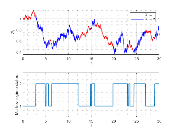
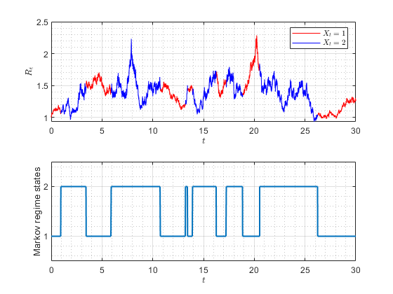
To simulate a sample path with 10,000 time steps, parameters for process (5) are set as follows: , , , , , and . For process (6), the parameters are chosen as , , , , , and . Both processes begin in state , with and . In Figure 1, red lines mark intervals when the processes are in state 1, while blue lines represent intervals in state 2. Two scenarios are depicted: in the time interval , process (5) switches states seventeen times, whereas process (6) switches twelve times.
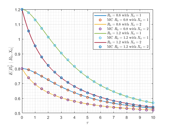
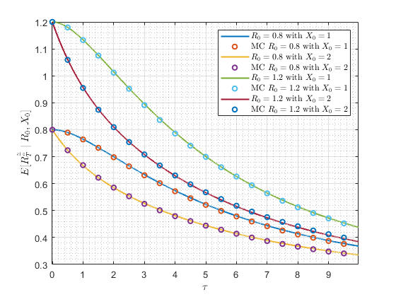
It is interesting to determine the effectiveness of our method compared to the regime-switching model and some other well-known models. The comparisons with relative difference for as displayed in Figures 2 and 3.
when and .
when and .
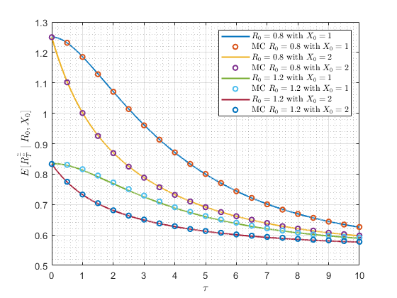
when and .
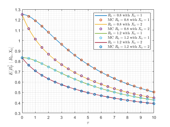
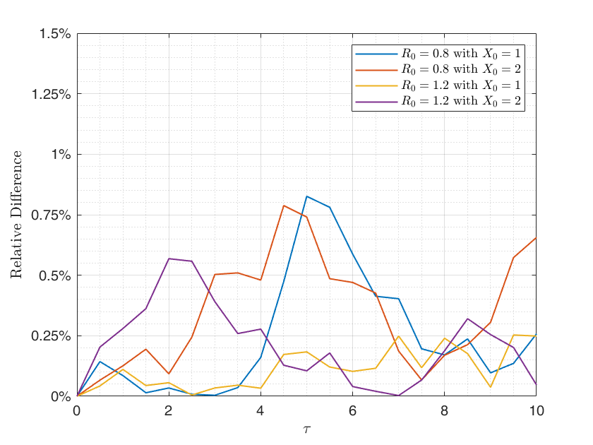
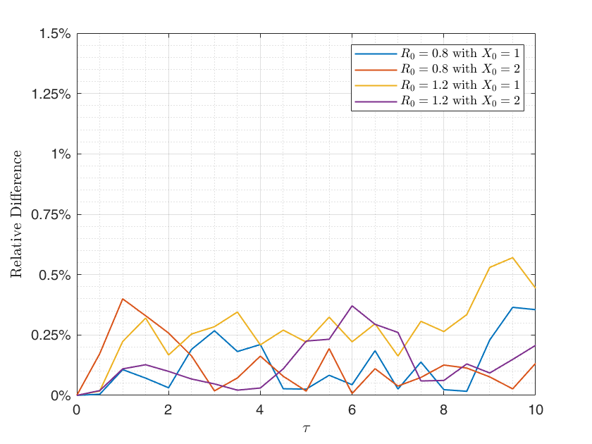
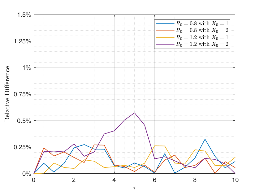
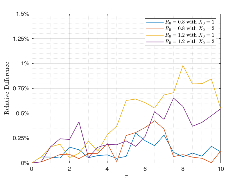
Figures 2 and 3 show that the results obtained from both the closed-form solution and the Monte Carlo simulations align precisely with the relative difference no greater than 1.00%. This indicates that our closed-form formulas, utilized for computing the conditional moments in Theorems 3 and 6, do not contain any algebraic errors.
5 Financial applications on VIX option pricing
The VIX, a 30-day implied volatility measure derived from S&P 500 index options, is essential for assessing market sentiment and managing volatility risk. Accurate pricing of VIX derivatives depends on using a model that captures the complex nature of volatility. This study presents a novel approach to VIX option pricing, introducing a closed-form formula based on the NLD-CEV model with regime switching. The NLD-CEV model offers several advantages over traditional models, such as the Cox–Ingersoll–Ross (CIR) model, by incorporating mean reversion and enabling data-driven estimation of the elasticity parameter . This flexibility addresses a key limitation of commonly used models like the square root and 3/2 models, which assume fixed values of at 1 and 3, respectively. Empirical evidence suggests that often falls outside this range, underscoring the need for a model that allows for data-driven parameter estimation [17, 18].
Leveraging the theoretical basis of the NLD-CEV model, this research develops a VIX option pricing formula with practical implications. The ability to derive a closed-form solution for fractional-order conditional moments in the NLD-CEV process enables efficient and accurate option price calculations. This methodology bridges the gap between advanced mathematical modeling and practical financial applications, significantly enhancing option pricing techniques for volatility derivatives.
This section applies the derived closed-form formula to price VIX options within a 2-state regime-switching NLD-CEV framework. The focus is on European call options on the VIX index, a critical tool in volatility trading and risk management. Consider a European call option with maturity date and strike price . The fair value of this option at any time is defined by
| (38) |
where is the risk-free rate, denotes the time to maturity, represents the VIX level at time , and indicates the regime state at time .
To efficiently compute the expectation in Equation (38), the Laguerre expansion method by Dufresne [19] is employed. This approach expresses the European call option price as an infinite series,
| (39) |
where satisfy , and denotes the generalized Laguerre polynomial of order with parameter . The coefficients are given in terms of the conditional moments of ,
| (40) |
for , where . Implementing this option pricing formula involves several steps. First, suitable values for and are chosen to satisfy and ensure that for all . This choice of parameters guarantees the convergence of the Laguerre series and facilitates calculation of the coefficients. Next, the closed-form formula for the NLD-CEV process expectation is used to obtain the moments . These moments are subsequently applied to calculate the coefficients in (40). Finally, the option price is computed using a truncated version of the series in (39).
This method provides substantial benefits in VIX option pricing, including fast computation and high accuracy enabled by closed-form solutions. By aligning with the NLD-CEV framework, this approach ensures that the option pricing model accurately reflects the VIX dynamics. Applying these theoretical findings to a practical quantitative finance problem demonstrates potential improvements in pricing and hedging strategies for volatility trading and risk management. This work advances the development of sophisticated option pricing methodologies, linking rigorous mathematical modeling with tangible financial applications.
6 Conclusion and discussion
In this study, we presented an analytical framework for the fractional-order conditional moments of the NLD-CEV process with regime-switching dynamics. By integrating a nonlinear drift component and accommodating elasticity in variance, our approach offers a versatile modeling tool for financial markets, especially in pricing derivatives like VIX options, where volatility and market shifts play critical roles. The hybrid system approach adopted here allows for exact closed-form solutions, which significantly enhances computational efficiency compared to traditional Monte Carlo simulations.
Our numerical results underscore the computational advantages of the closed-form formulas derived in this study. In particular, we observe substantial reductions in computational time, with accuracy that aligns closely with MC simulation outcomes. This computational efficiency is invaluable in practical applications where rapid pricing and risk assessment are essential. Furthermore, our results demonstrate that the NLD-CEV model captures nuanced dynamics by adjusting to changes in economic conditions through regime-switching, thereby providing more accurate reflections of market realities than many traditional models.
The applications explored, specifically in VIX options and options pricing, highlight the practical utility of our model in financial engineering. The model’s adaptability to shifts in market sentiment and volatility makes it well-suited for environments characterized by sudden economic changes. By incorporating regime-switching elements, the NLD-CEV model not only enhances accuracy in volatility modeling but also addresses some limitations inherent in simpler processes by capturing nonlinear responses to market shocks.
Future research could extend this work by exploring multi-regime settings and incorporating additional stochastic elements to further refine the model’s adaptability to market complexities. Additionally, empirical validation using a broader dataset of financial instruments could provide insights into optimizing model parameters for specific financial contexts. This research contributes a significant step toward more efficient and accurate pricing methodologies, bridging advanced stochastic modeling techniques with concrete financial applications.
References
- [1] John Cox. Notes on option pricing I: Constant elasticity of variance diffusions. Unpublished note, Stanford University, Graduate School of Business, 1975.
- [2] Axel A Araneda and Nils Bertschinger. The sub-fractional cev model. Physica A: Statistical Mechanics and its Applications, 574:125974, 2021.
- [3] Jiling Cao, Jeong-Hoon Kim, and Wenjun Zhang. Pricing variance swaps under hybrid cev and stochastic volatility. Journal of Computational and Applied Mathematics, 386:113220, 2021.
- [4] Terry A Marsh and Eric R Rosenfeld. Stochastic processes for interest rates and equilibrium bond prices. The Journal of Finance, 38(2):635–646, 1983.
- [5] Phiraphat Sutthimat, Khamron Mekchay, and Sanae Rujivan. Closed-form formula for conditional moments of generalized nonlinear drift CEV process. Applied Mathematics and Computation, 428:127213, 2022.
- [6] Hao Zhou. Itô conditional moment generator and the estimation of short-rate processes. Journal of Financial Econometrics, 1(2):250–271, 2003.
- [7] Dong-Hyun Ahn and Bin Gao. A parametric nonlinear model of term structure dynamics. The Review of Financial Studies, 12(4):721–762, 1999.
- [8] Lech A Grzelak and Cornelis W Oosterlee. On the Heston model with stochastic interest rates. SIAM Journal on Financial Mathematics, 2(1):255–286, 2011.
- [9] Sanae Rujivan and Song-Ping Zhu. A simple closed-form formula for pricing discretely-sampled variance swaps under the heston model. The ANZIAM Journal, 56(1):1–27, 2014.
- [10] SP Mirevski and L Boyadjiev. On some fractional generalizations of the Laguerre polynomials and the Kummer function. Computers & Mathematics with Applications, 59(3):1271–1277, 2010.
- [11] Sanae Rujivan, Athinan Sutchada, Kittisak Chumpong, and Napat Rujeerapaiboon. Analytically computing the moments of a conic combination of independent noncentral chi-square random variables and its application for the extended Cox–Ingersoll–Ross process with time-varying dimension. Mathematics, 11(5):1276, 2023.
- [12] Nicholas A Baran, George Yin, and Chao Zhu. Feynman–Kac formula for switching diffusions: connections of systems of partial differential equations and stochastic differential equations. Advances in Difference Equations, 2013:1–13, 2013.
- [13] Nicholas A Baran, George Yin, and Chao Zhu. Feynman–Kac formula for switching diffusions: connections of systems of partial differential equations and stochastic differential equations. Advances in Difference Equations, 2013:1–13, 2013.
- [14] Jay A Wood. The chain rule for matrix exponential functions. The College Mathematics Journal, 35(3):220–222, 2004.
- [15] Roudy El Haddad. Repeated Integration and Explicit Formula for the -th Integral of . arXiv preprint arXiv:2102.11723, 2021.
- [16] Chenggui Yuan and Xuerong Mao. Convergence of the Euler–Maruyama method for stochastic differential equations with Markovian switching. Mathematics and Computers in Simulation, 64(2):223–235, 2004.
- [17] Brice Dupoyet, Robert T Daigler, and Zhiyao Chen. A simplified pricing model for volatility futures. Journal of Futures Markets, 31(4):307–339, 2011.
- [18] Zhigang Tong. Modelling vix and vix derivatives with reducible diffusions. International Journal of Bonds and Derivatives, 3(2):153–175, 2017.
- [19] Daniel Dufresne. Laguerre series for asian and other options. Mathematical Finance, 10(4):407–428, 2000.