Transforming Engineering Diagrams:
A Novel Approach for P&ID Digitization using Transformers

Abstract

The digitization of complex technical systems, such as Piping and Instrumentation Diagrams (P&IDs), is crucial for efficient maintenance and operation of complex systems in hydraulic and process engineering. Previous approaches often rely on separate modules that analyze diagram elements individually, neglecting the diagram’s overall structure. We address this limitation by proposing a novel approach that utilizes the Relationformer, a state-of-the-art deep learning architecture, to extract graphs from P&IDs. Our method leverages the ability of the Relationformer to simultaneously detect objects and their relationships in images, making it suitable for the task of graph extraction from engineering diagrams. We apply our proposed approach to both real-world and synthetically created P&ID datasets, and evaluate its effectiveness by comparing it with a modular digitization approach based on recent literature. We present PID2Graph, the first publicly accessible P&ID dataset featuring comprehensive labels for the graph structure, including symbols, nodes and their connections that is used for evaluation. To understand the effect of patching and stitching of both of the approaches, we compare values before and after merging the patches. For the real-world data, the Relationformer achieves convincing results, outperforming the modular digitization approach for edge detection by more than 25%. Our work provides a comprehensive framework for assessing the performance of P&ID digitization methods and opens up new avenues for research in this area using transformer architectures. The P&ID dataset used for evaluation will be published and publicly available upon acceptance of the paper.

1 Introduction

The design process of complex technical systems starts with a conceptual engineering drawing that describes the properties of hydraulic components and instrumentation as well as their interconnections. These properties and relationships can be represented by an attributed, directed graph or relational structured data formats. Machine-readable information about technical systems can be used to support planning and operation of these systems through simulation using state-of-the-art frameworks. Nowadays, such plans are created digitally using CAD software and stored as machine-readable data. However, there is a large old stock of such plans in non-digital form. Furthermore, the exchange of such plans often takes place via rendered images or PDF files. This is linked to a rising demand for digitization of such documents. One type of diagrams are Piping and Instrumentation Diagrams (P&ID). A P&ID is a detailed diagram used in the chemical process industry, which describes the equipment installed in a plant, along with instrumentation, controls, piping etc. and is used during planning, operation and maintenance [34].

This paper presents several contributions to the field of P&ID digitization. Firstly, we describe methods for digitizing P&IDs based on a recent Transformer Network along with the Modular Digitization Approach based on previous work. We describe the metrics used for evaluating the performance of our proposed method, providing a comprehensive framework for assessing its effectiveness. We then compare our proposed methods using synthetically created engineering diagrams and engineering diagrams from a real-world system. To facilitate further research and development, we publish the small test dataset PID2Graph. Notably, this dataset is, to the best of our knowledge, the first publicly available P&ID dataset that contains real-world data and annotations for the full graph, including symbols and their connections.

2 Related Work

Engineering diagram digitization primarily involves two key tasks: extracting components and their interconnections. The successful digitization of Piping and Instrumentation Diagrams (P&IDs) enables the automated creation of accurate simulation models, as demonstrated by previous research. For instance, Paganus et al. [25] generated models from text-based descriptions, while Stürmer et al. [32] developed a pipeline for generating simulation models directly from digitized engineering diagrams. P&ID digitization can be approached in two ways: as a series of separate sub-problems solved by one module per sub-problem or as an image-to-graph problem.

2.1 Modular Engineering Diagram Digitization

The most commonly employed method to digitize P&IDs is utilizing separate deep learning models or algorithms for symbol detection, text detection, and line detection. The connection detection usually is not evaluated. This approach was first proposed by Rahul et al. [29] and has since been refined in subsequent work [21, 9]. Here, Convolutional Neural Networks (CNN) are employed for symbol and text detections. Afterwards, probabilistic hough transform or other traditional computer vision algorithms are applied to detect lines. To combine these detections, a graph describing the components and their interconnections is created. A recent review by Jamieson et al. [13] provides an in-depth analysis of existing literature on deep learning-based engineering diagram digitization. In contrast to employing CNNs for symbol detection (e.g., [23, 7]), alternative approaches have been explored, including the use of segmentation techniques [22] or Graph Neural Networks (GNNs) [27]. Additionally, other studies have focused on related but distinct tasks, such as line and flow direction detection [15] or line classification [16].

The principles of engineering diagram digitization can be extended to other domains, even if the application domain or diagram type differs from P&IDs. A recent study by Theisen et al. [33] has demonstrated the digitization of process flow diagrams (PFDs), leveraging a dataset comprising approximately 1,000 images sourced from textbooks. The connections and graph were extracted by skeletonizing the image. However, the connection extraction was not evaluated due to missing labels for this task. Other approaches deal with electrical engineering diagrams [4, 37], handwritten circuit diagram digitization [2], mechanical engineering sketches [6] or construction diagrams [14].

2.2 Image to Graph

Another possibility to tackle engineering diagram digitization is framing it as an image-to-graph problem. He et al. [10] introduce a road graph extraction algorithm that is able to extract a graph describing a road network from satellite images using neural networks. A similar problem is described by Belli et al. [3], where a Generative Graph Transformer is described to extract graphs from images of road networks. Although the problem of identifying connections in diagrams is similar to extracting connections from engineering diagrams, the challenges of identifying specific symbols and extracting different types of relationships remain. The Scene Graph Generation (SGG) task involves solving these challenges, where objects from an image are extracted and the relationships between them are determined [38]. One transformer network dealing with SGG is SGTR+ [18]. A recent framework combining SGG and road network extraction is the Relationformer proposed by Shit et al. [31]. The Relationformer, an enhancement of deformable DETR (DEtection TRansformer) [39], combines advanced object detection with relation prediction and is shown to outperform existing methods. Since its release, the Relationformer has successfully been adapted for further work like crop field extraction [36]. Metrics that have been used to evaluate graph extraction evaluation are manifold. For the problem of road network extraction from images, the metrics Streetmovers-Distance [3], TOPO [5, 3] or APLS Metric [35] were introduced. Another commonly used relation metric is the scene graph generation metric $\text{mR@}K$. Objects are matched by IOU (or similar metrics) and the (object, relation, object)-tuples are ranked by confidence. The $K$ most confident results are then used to calculate the mean recall. For scene graph generation, this approach with using only the top-$K$ results is used because the annotations are highly incomplete due to the high amount of possible relations. [19]

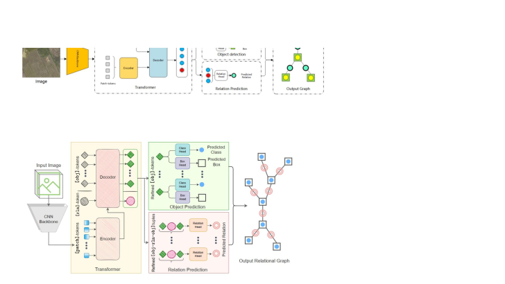
Figure 1: Overview of the Relationformer [31] and the Modular Digitization Approach to digitize engineering diagrams. The preprocessing step patches and adjusts the data, which is then fed into each method to produce a graph representation as output.

2.3 Datasets

Developing effective models for P&ID digitization requires P&IDs that are accurately labeled with symbols and connections. Unfortunately, existing research has mostly been evaluated on private datasets not made publicly available due to concerns around copyright and intellectual property rights. Some approaches use synthetic data [23, 26] or augment their data applying Generative Adversarial Networks (GANs) [8]. The only published dataset for P&ID digitization is Dataset-P&ID by Paliwal et al. [26] consisting of 500 synthetic P&IDs with 32 different symbol classes. The data includes annotations for symbols, lines, and text, which are valuable resources. However, the graph structure annotations are not provided, and the lines between symbols are drawn using a simplified grid layout. Additionally, one lines style can change between dashed and solid forms. These limitations may impact the effectiveness of certain models or methods trained or evaluated with this dataset.

3 Methods

Due to its supposed ability to be adaptable, we apply the Relationformer model in the context of engineering diagram digitization, and compare it to a method that breaks down the digitization task into separate sub-tasks of detecting symbols, text, lines, and then extracting graphs, referred to as Modular Digitization Approach in this paper. Both the proposed Relationformer and the Modular Digitization Approach share a common goal of identifying and classifying symbols and lines within P&IDs. Their outputs are unified in the form of a graph representation, where each node contains a bounding box and symbol class, while edges have an edge class. The models will be trained and evaluated with the classes listed in Tab. 1, i.e. seven symbol classes and two line classes. The workflow for the preprocessing step and both methods is visually depicted in Fig. 1 and are discussed in detail in the subsequent sections.

3.1 Preprocessing

Due to the high resolution of P&IDs alongside with big size differences between symbols, the input resolution for the models would have to be high in order to still accurately depict symbols and lines. We use patching to split the full diagram resized to 4500x7000 into multiple patches with an overlap of at least $50\text{\,}\mathrm{\char 37\relax}$. During both model processing steps, each patch is independently processed and then combined with its neighbors to form a complete graph representation.

Table 1: Classes of symbols and edges used for training and evaluation.

Symbols			Lines
General	Pump/Compressor	Arrow	Solid
Tank/Vessel	Instrumentation	Inlet/Outlet	Non-Solid
Valve

3.2 Relationformer

The Relationformer is described as in the original paper [31] and implemented in a modified form to adapt to P&IDs. The Relationformer is based on deformable DETR [39] and consists of a CNN backbone, a transformer encoder-decoder architecture and heads for object detection and relation prediction (see Fig. 1). The main difference to deformable DETR is the decoder architecture and the relation prediction head. The decoder uses $N+1$ tokens as the first input, where $N$ is the number of object-tokens and a single relation-token. The second input are the contextualized image features from the encoder. The objection detection head consists of two components. Firstly, Fully Connected Networks (FCNs) are employed to predict the location of each object within the image, in form of a bounding box that define the spatial extent of each object. Secondly, a single layer classification module is used, assigning a class label to each detected object. Thus, the output of the object detection head consists of the class and bounding box of the object. The relation prediction head has a pairwise object-token and a shared relation-token, where a multi layer-perceptron (MLP) predicts the relation $\tilde{e}^{ij}_{\text{rln}}=\text{MLP}_{\text{rln}}({o^{i},r,o^{j}}_{i\neq j})$ for every object-token pair $o^{i}$ and $o^{j}$ with the relation-token $r$.

According to [31], the loss function for training the Relationformer includes the object detection regression (reg) and classification (cls) losses as well as global intersection over union (gIoU) loss and the relation loss (rln) with their respective weighting factors $\lambda$ and is given by Eq. 1.

$$\mathcal{L}_{total} =\sum_{i=1}^{N}[\mathbbm{1}_{v^{i}_{\text{cls}}\notin\varnothing}(\lambda_{\text{reg}}\mathcal{L}_{\text{reg}}(\boldsymbol{v}_{\text{box}}^{i},\tilde{\boldsymbol{v}}_{\text{box}}^{i})$$ (1)

$$+\lambda_{\text{gIoU}}\mathcal{L}_{\text{gIoU}}(\boldsymbol{v}_{\text{box}}^{i},\tilde{\boldsymbol{v}}_{\text{box}}^{i}))]$$

$$+\lambda_{\text{cls}}\sum_{i=1}^{N}\mathcal{L}_{\text{cls}}(v_{\text{cls}}^{i},\tilde{v}^{i}_{\text{cls}})$$

$$+\lambda_{\text{rln}}\sum_{{i,j}\in\mathcal{R}}\mathcal{L}_{\text{rln}}(e_{\text{rln}}^{ij},\tilde{e}_{\text{rln}}^{ij})$$

The bounding box coordinates are given as $\boldsymbol{v}_{\text{box}}^{i}$ for the ground truth and as $\tilde{\boldsymbol{v}}_{\text{box}}^{i}$ for the prediction. Objects are matched with the Hungarian matching algorithm [17]. If they have a relation, the relation is classified as ’valid’ and otherwise ’background’. As there is a connection from every object to every other object, the number of relations that is of the ’background’ kind would dominate over ’valid’ relations, which is why $\mathcal{R}$ is describing only a subset of the relations between the $i$-th to the $j$-th object, where only three random ’background’ relations are sampled for each ’valid’ relation.

To adapt the Relationformer model for training on the patched data, several modifications were made to the input graph. In addition to the pre-existing symbol classes, new node categories were introduced to capture key features of the diagram’s structure: line ankles, crossings and borders. Nodes get appended to the graph accordingly with a bounding box around the center of the node that has a uniform size, analogously to the procedure described in the original Relationformer paper regarding road networks. A border bounding box is created when a line gets cut during patching at the position where the line intersects the border of the patch. Examples for this patched images and graphs can be seen in Fig. 2.

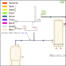
(a)

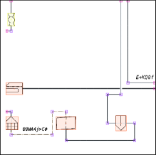
(b)

Figure 2: Two example patches obtained after dividing the full diagram of OPEN100 (a) and the Synthetic Test Data (b), with border nodes (pink) and bounding boxes (several colors) marking where lines exit each patch. These patches serve as input to the Relationformer for training, testing and evaluation.

Afterwards, the predicted graphs for single patches are merged into a graph representing the complete plan. The merge process consists of the following steps:

1. Lowering the confidence score for each bounding box in a patch with the function $\hat{c}=c-\alpha\cdot e^{-3|d\frac{2}{S}|}$, where $\hat{c}$ is the modified confidence score, $c$ is the original confidence score, $S$ is the size of the patch, $d$ is the smallest distance between the bounding box and the patch border and $\alpha$ is the maximal amount of the weighting $\alpha=0.4$. Therefore, symbols with bounding boxes closer to the patch border are more likely to be cut off, as there is a possibility the same symbols is included to a bigger extent in another patch;

2. Filtering predictions with a low confidence score in order to ignore them during the merging process;

3. Collecting and resizing all bounding boxes for the complete plan;

4. Non-maximum suppression (NMS) with a high IOU threshold to merge duplicates;

5. Weight-boxed fusion (WBF) with a lower IOU threshold to combine information from bounding boxes;

6. Cleaning up the graph by removing self-loops and non-connected nodes.

3.3 Modular Digitization Approach

An alternate, more commonly used approach involves separately detecting symbols, text and lines and then merging them together into a graph, following earlier work of Stürmer et al. [32], as can be seen in Fig. 1.

Symbol Detection

The first step in this process is detecting symbols. An improved Faster R-CNN [20] approach is trained to do this. The patching and merging of the input data is done as described in Sec. 3.2. Because no graph structure is considered by this object detector, the classes for crossings, ankles and border nodes do not exist.

Text Detection

In addition to symbol detection, text within the diagram is identified, including labels, notes and text inside of symbols and tables. CRAFT [1] as implemented in EasyOCR [12] is used to achieve this. It can handle text in various languages, fonts and styles, making it versatile for different types of diagrams. The output of CRAFT consists of bounding boxes containing text. Notably, this text detection functionality serves as an auxiliary mechanism for filtering purposes only, rather than being evaluated. Filtering text prevents the line detection module from incorrectly classifying textual elements as graph connections.

Line Detection

The third component of this pipeline is the detection of straight lines and identification of multiple smaller segments belonging to dashed lines. Bounding boxes resulting from symbol- and line detection are used to filter out elements from the graph that are not connecting symbols. Horizontal and vertical lines are detected through the application of dilation and erosion operations, followed by the calculation of their convex hulls. Furthermore, line thinning and Progressive Probabilistic Hough Transform are used to detect non-vertical and non-horizontal lines that were not detected before. Small line segments are assumed to be dashes of a dashed line. To reconstruct the dashed lines, the dashes are clustered using the DBSCAN algorithmus and merged together.

Graph Generation

The final step is the generation of a comprehensive graph, which brings together detected symbols and lines. To achieve this, we assign start and end points of a detected line to either the closest symbol or the nearest corresponding point of another line. If three or more lines have their start or end points connected, a crossing node is created. If there is an ankle between two linked line segments, an ankle node is created. The resulting graph is then refined (in the same way as the Relationformer) by removing self-loops and unused nodes.

3.4 Datasets

To address the gap of missing complex and real-world datasets, we have created our own datasets with detailed annotations for symbols and connections. The synthetic data is generated using templates scrambled and cutout from P&ID standardization and legends. Our algorithm randomly places these templates on a canvas and connects them in a way that forms a connected graph. If lines intersect, a crossing node is created. Furthermore, this data includes various line types, such as solid and dashed lines, to enhance the realism of our digitization task and add data diversity. To further simplify the data and focus on the essential graph structure, additional information such as tables, legends and frames are removed. The patched training dataset is augmented with various transformations, comprising small angle rotations, $90\text{\,}\mathrm{\SIUnitSymbolDegree}$ rotations, horizontal and vertical flips, minor adjustments to brightness and contrast, random scaling, and image blurring.

The training data consist of synthetic and real-world data. Synthetic 700 is a synthetic dataset with 700 different symbol templates collected from a broad range of sources. Additionally, we have manually annotated 60 real-world P&IDs from various plants.

For the PID2Graph Synthetic data, synthetic plans with only symbols from [30] based on ISO 10628 [11] are included.

PID2Graph OPEN100 is used to further validate our method. It includes 12 manually annotated publicly available P&IDs from the OPEN100 reactor [24]. Notably, these plans do not contain dashed lines, allowing us to assess the robustness of our model in a scenario where this feature is absent.

To enable a comparison with previous work, we also evaluate our methods on Dataset-P&ID from Paliwal et al. [26]. This dataset includes annotations in the form of bounding boxes for 32 different symbols and start and end points of line segments, rather than in a graph format. We convert these annotations to align with the format used in our other datasets. Specifically, we map the 32 symbol classes to our classes as outlined in Table 1, and we connect overlapping line segments to create edges. Since these edges may include both dashed and solid segments, we assign a unified edge label across all edges.

An in depth comparison of the datasets can be found in Sec. S3 in the supplementary material.

3.5 Metrics

We evaluate the quality of graph construction using conventional object detection metrics, where each detected bounding box corresponds to a node in the graph along with a metric for measuring edge detection performance.

3.5.1 Node Detection

To comprehensively measure the performance of our method in constructing graph nodes, we employ two metrics. Firstly, mean Average Precision (mAP) is used to evaluate the estimation of individual symbols, considering only classes from Tab. 1 that do not involve crossings and ankles, as these categories relate to graph connectivity rather than symbol representation.

The second metric used is average precision (AP) across all symbols, crossings and ankles. However, unlike the first metric, each symbol is assigned to the same class, because an error or a confusion in the assignment of the class to a node is not decisive for the entire graph reconstruction, as long as the node exists. This allows us to evaluate the consistency and accuracy of our method in constructing the graphs structure. Both metrics are calculated using an Intersection over Union (IOU) threshold of $0.5$. We choose this threshold because exact bounding box localization is not crucial for our application.

3.5.2 Edge Detection

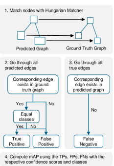
Figure 3: Description of the implemented metric for calculating the edge mAP.

Line detection describes the task of detecting the position of a line in the pixel space and it’s type, which is used by previous approaches. In contrast, edge detection is the task of detecting edges between two objects or nodes. An edge detection metric should reflect the task as independently as possible from node detection. This is inherently difficult, because an edge is always associated with two nodes. If one of the nodes is missing, the edge will be missing as well. For a false positive node, there may be edges connected to that node that would never exist if the node had not been detected in the first place. Several commonly used metrics are described in Sec. 2.2. However, the length of lines on a P&ID diagram does not necessarily correlate with the actual length of pipes or other components, and thus the metrics for road network extraction is not suitable to evaluate the quality of reconstructed graphs in this domain. In case of the engineering diagram digitization, where the connections are distinct and finite, $\text{mR@}K$ is also not suited for the digitization problem. Thus, we propose a metric for edge detection mean Average Precision (edge mAP) using the Hungarian matching algorithm as depicted in Fig. 3. The Hungarian matching algorithm is used to solve assignment problems by optimally pairing elements from two sets while minimizing the overall cost to match nodes from one graph to another using the nodes bounding boxes to use the gIoU as the cost function. Average precision (AP) is calculated using the precision-recall curve. A detailed description of the algorithm for edge mAP computation is Algorithm S1 in the supplementary material.

The evaluation metric is illustrated through an example calculation in Fig. 4. This example demonstrates that the metric places greater importance on correctly predicted edges and nodes than on not predicted or wrongly predicted ones, particularly when such predictions are made adjacent to incorrectly detected crossing nodes.

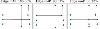
Figure 4: Exemplary values of the edge mAP metric with the ground truth graph on the left and two other graphs in the middle and on the right. The graph in the middle misses two edges, and the one on the right adds several edges by falsely predicted crossing nodes.

3.6 Model Training

The Relationformer and Faster R-CNN are trained on a mix of the Synthetic 700 data and real world P&IDs, as presented in Tab. 2. First, we pre-train both methods on a large set of $2000$ synthetic P&IDs, which are patched and augmented multiple times to create a vast pool of $170\,944$ samples for training and $8998$ samples for validation. Next, we fine-tune the models on a mix of the 60 real world P&IDs and a subset of 500 synthetic P&IDs. To increase the presence of real data in the training set, we augment each real world P&ID three times as much as each synthetic P&ID. This results in $44\,019$ samples for training and $2317$ samples for validation in the second training phase. Approximately 37% of the training set comprised patches from real-world data, while 63% consisted of patches from synthetic plans. During this second phase of training, we stop when either the loss stabilizes or the validation loss begins to rise, indicating potential overfitting. Additional training details are listed in the supplementary material.

Table 2: Amount of P&IDs and samples used for both training sets.

	Pre-Training Set	Training Set
Training Samples	$170\,944$	$44\,019$
Validation Samples	$8998$	$2317$
Real World P&IDs	0	$60$
Synthetic P&IDs	$2000$	$500$

4 Results

Table 3: Performance comparison of the Modular Digitization and Relationformer on both test sets with higher values highlighted as bold. As in the Modular Digitzation the graph construction is done after patch merging, no values can be given for node AP and edge mAP for patches.

	Modular Digitization								Relationformer
	Patched				Stitched				Patched				Stitched
	Symbols	Nodes	Edges		Symbols	Nodes	Edges		Symbols	Nodes	Edges		Symbols	Nodes	Edges
	mAP	AP	mAP		mAP	AP	mAP		mAP	AP	mAP		mAP	AP	mAP
PID2Graph OPEN100	86.58	-	-		76.99	52.14	45.89		73.49	82.18	76.79		73.14	83.63	75.46
PID2Graph Synthetic	78.74	-	-		74.15	85.16	50.26		78.62	87.44	93.86		78.36	96.89	88.95
Dataset-P&ID [26]	85.87	-	-		83.95	89.32	85.46		80.32	96.59	92.46		76.69	97.72	95.07

The results are presented in Tab. 3. Our experiments on the patched OPEN100 data with the Relationformer model demonstrate good performance in detecting symbols (73.49%), nodes (82.18%) and connections (76.79%). When evaluated on full plans, the performance stays the same (around 1% increase or decrease). For the synthetic data, the symbol detection mAP has similar values after stitching the patches, while the stitching has a significant influence on node and edge detection, rising the node AP by 9.45% to 96.89% and lowering the edge mAP by 4.91% to 88.95%. In contrast, the modular digitization shows a more moderate performance, achieving decent symbol detection on the OPEN100 data on patches (86.58%) but struggling with node detection (52.15%) and edge detection (45.89%), similar to its performance on synthetic data.

Both methods demonstrate strong results on Dataset-P&ID, with modular digitization again showing better values only for symbol detection.

To investigate the impact of larger symbols, we conducted experiments on the OPEN100 data using an enlarged patch size to encompass bigger symbols within a single patch. Additionally, we performed experiments on a subset of the OPEN100 data that consisted only of plans where all symbols could be accommodated entirely within a patch. The results can be seen in Tab. 4. When increasing patch size from originally (1500, 1500) to (2000, 2000), which should facilitate better inclusion of larger symbols, the symbol and node detection value of the Relationformer drop by at least 10%, while the values of the Modular Digitization stay around the same. When using the small symbol subset, both methods show improved performance, with a gain of 9.49% for symbol detection by the Relationformer and 10.49% by the Modular Digitization. Moreover, the results show that the Modular Digitization’s performance drops significantly from patched to stitched on the full OPEN100 data. However, its performance increases when using only the subset with small symbols. This suggests that the stitching process struggles with larger symbols.

Table 4: Ablation studies for the Relationformer and Modular Digitization for the OPEN100 data on different patch sizes and a test subset containing only objects that fit into a patch completely.

	Data	Patch Size	Symbols	Nodes	Edges
			mAP	AP	AP
	Patched	(2000, 2000)	86.52	-	-
Modular Digitization	Stitched	(2000, 2000)	76.74	57.49	55.08
	Patched, Small Symbol Subset	(1500, 1500)	86.51	-	-
	Stitched, Small Symbol Subset	(1500, 1500)	87.48	62.26	53.95
	Patched	(2000, 2000)	62.23	50.11	69.88
Relation$-$ former	Stitched	(2000, 2000)	62.42	56.15	67.67
	Patched, Small Symbol Subset	(1500, 1500)	80.07	82.90	73.08
	Stitched, Small Symbol Subset	(1500, 1500)	82.74	83.80	75.16

The performance of the Relationformer on the OPEN100 data is further investigated by examining the confusion matrix in Fig. 5. Notably, the ’general’ class exhibits a high degree of confusion, with pumps being frequently misclassified as symbols belonging to this category. The confusion with the ’general’ class is consistent with the other datasets (see Sec. S4 in the supplementary material for the remaining confusion matrices).

To gain a better understanding of the detection capabilities and graph reconstruction quality, we have also visually inspected the predictions. Fig. 6 illustrates the merged graph for an entire plan. Overall, the graph is correctly constructed, though there are some noticeable misclassifications of instrumentation symbols and additional false positive diagonal connections between crossings and symbols. More detection examples are included in Sec. S6 in the supplementary material.

5 Discussion

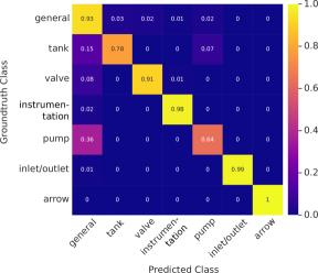
Figure 5: Confusion matrix for the stiched symbol detection results of the Relationformer for the OPEN100 data.

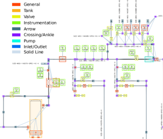
Figure 6: Extract of a digitization result of the Relationformer for one merged P&ID from the OPEN100 test data. The legend shows the class names of the predictions.

The Relationformer shows good results on every task, while the Modular Digitization shows especially bad results on the edge detection. The results highlight several challenges that need to be addressed in order to achieve accurate graph reconstruction and relation detection. The symbol detection module of the Modular Digitization however achieves better performance in correctly classifying symbols on the OPEN100 data.

The Modular Digitization has the disadvantage of being highly dependent on previous steps, where each step, especially line detection, is reliant on using good parameters. The Relationformer enables end-to-end training without significant adjustment after training. This property is expected to facilitate good generalization across different domains.

One of the primary difficulties lies in the patching and merging process. Errors occurred during the patching process itself, resulting in incorrect input data for our models used for training. When splitting the P&ID diagrams into patches, this can lead to the truncation of symbols. When only a fragment of a symbol remains, it can be difficult to distinguish it from other symbols or even lines, making it difficult for our models to train and evaluate on this data.

A problem with detecting symbols and differentiating between classes is the ”general” class. This class encompasses a diverse range of symbols, resulting in high intra-class variation. As a consequence, models struggle to generalize effectively across these disparate symbols, making evaluation and pinpointing specific issues within this category more challenging. The confusion matrices of the Relationformer support this assertion, as the general class is the class with the highest confusion across all datasets. The general detection and localization of symbols appear to be quite effective, as indicated by high node AP scores. However, improving the classification of symbols not seen during training and assigning more specific labels remains a focus for future work.

The metrics applied are based on classical symbol detection techniques and include a custom-defined metric. We used an IoU threshold of 0.5 to evaluate our methods, which is relatively low compared to other object detection tasks. A potential challenge in using a higher IoU threshold lies in the uncertainty of manually annotated data, as these annotations are less precise than the automatically generated bounding boxes for synthetic data. The utility of the edge metric warrants consideration, since it disproportionately penalizes incorrect edge predictions compared to missed edges. Furthermore, the edge detection metric relies on accurately matching nodes between the ground truth and predicted graphs based on bounding boxes. However, if a method accurately predicts edges, the metric will reflect this performance appropriately.

Additionally, our study underscores the importance of collecting and utilizing larger datasets with real-world diagrams including big symbols. Even though dashed or non-continuous lines are not present in the OPEN100 data, the results on the synthetic data suggests that the Relationformer is also able to classify line types accurately.

6 Conclusion

In this study, we address the challenge of digitizing engineering diagrams of complex technical systems, specifically Piping and Instrumentation Diagrams (P&IDs). Leveraging the state-of-the-art Relationformer architecture, we propose a novel approach that simultaneously detects objects and their relationships from engineering diagrams. Our methods not only detect bounding boxes and lines, but extract a graph describing the system and its structure. We demonstrate the effectiveness of our method on both real-world and synthetically created P&ID datasets, achieving superior results compared to a modular digitization approach. The dataset used for evaluation is made publicly available. The achieved metrics for node detection (83.63% AP) and edge detection (75.46% edge mAP) showcase the potential of transformer architectures in this domain.

Supplementary Material

S1 Edge Metric Calculation

We calculate the metric for edge detection mean Average Precision (mAP) as described in Algorithm S1. The Hungarian matching algorithm [17] is used to match nodes (mapping $M$) from the ground truth graph $G_{\text{true}}$ to the predicted graph $G_{\text{pred}}$ using the nodes (denoted with $V$) bounding boxes. All edges $e_{u,v}$ from node $u$ to node $v$ of the predicted graph have a confidence score and a class. An edge $e_{\hat{u},\hat{v}}$ is an edge in the ground truth graph and also has a class. The average precision function from the Python library scikit-learn [28] is used to calculate the average precision.

Algorithm S1 Edge mAP Computation

1:Input: $G_{\text{true}}(V_{\text{true}},E_{\text{true}})$, $G_{\text{pred}}(V_{\text{pred}},E_{\text{pred}})$

2:Initialize:

3:$(\text{TP, FP, FN})\leftarrow(\text{empty list, empty list, empty list})$

4:$M\leftarrow$ HungarianMatcher($V_{\text{true}},V_{\text{pred}}$) $:V_{\text{true}}\to V_{\text{pred}}$

5:for each predicted edge $e_{u,v}\in E_{\text{pred}}$ do

6:       $e_{\hat{u},\hat{v}}$ $\leftarrow$ $e_{M^{-1}(u),M^{-1}(v)}$

7:       if $e_{\hat{u},\hat{v}}\in E_{\text{true}}$ then

8:             if class($e_{u,v}$) = class($e_{\hat{u},\hat{v}}$) then

9:                    TP.insert($(\text{class}(e_{u,v}),\text{conf\_score}(e_{u,v}))$)

10:             else

11:                    FP.insert($(\text{class}(e_{u,v}),\text{conf\_score}(e_{u,v}))$)              

12:       else

13:             FP.insert($(\text{class}(e_{u,v}),\text{conf\_score}(e_{u,v}))$)        

14:for each true edge $e_{\hat{u},\hat{v}}\in E_{\text{true}}$ do

15:       $e_{u,v}\leftarrow e_{M(\hat{u}),M(\hat{v})}$

16:       if $e_{u,v}\notin E_{\text{pred}}$ then

17:             FN.insert($\text{class}(e_{\hat{u},\hat{v}})$)        

18:$\text{mAP}_{\text{edge}}\leftarrow\frac{1}{|\text{classes}|}\sum_{c\in\text{classes}}\text{AP}_{c}(\text{TP, FP, FN})$

19:Return: $\text{mAP}_{\text{edge}}$

S2 Training

The relevant hyperparameters can be seen in Tab. S1 and Tab. S2. For both Relationformer and Faster R-CNN with the Modular Digitization, we employ a 0.95:0.05 training-validation split, allocating the majority of the data to training. This partitioning is deliberate, given the transformer network’s propensity for requiring substantial amounts of data to achieve good performance.

Table S1: Hyperparameters used to train the Relationformer.

Hyperparameter	Value
Batch Size	20
Image Size	(512, 512)
Epochs	80
Learning Rate	1e-4
Learning Rate Backbone	3e-5
Number of Queries	401
Backbone	ResNet-101
$\lambda_{\text{box}}$	2
$\lambda_{\text{cls}}$	2
$\lambda_{\text{card}}$	1
$\lambda_{\text{node}}$	4
$\lambda_{\text{edge}}$	3
Randomize Edge Directions	Yes

Table S2: Hyperparameters used to train Faster R-CNN for symbol detection.

Hyperparameter	Value
Batch Size	16
Image Size	(1024, 1024)
Epochs	40
Learning Rate	5e-4

Table S3: Dataset statistics prior to splitting and augmentation. Real-world P&IDs exhibit significantly higher data variability compared to synthetic counterparts.

	# of Nodes per Plan	# of Edges per Plan	# of Symbols, Crossings & Ankles	# of Edges	Symbol Area (px) Mean ± Std	Usage
Synthetic 700	$131$ ± $14$	$133$ ± $15$	$183\,901$	$188\,550$	$6071$ ± $22\,059$	Train
Real World	$497$ ± $338$	$457$ ± $338$	$17\,218$	$14\,649$	$5776$ ± $54\,328$	Train
Dataset-P&ID	$452$ ± $86$	$505$ ± $91$	$51\,182$	$137\,449$	$3350$ ± $4291$	Test
PID2Graph Synthetic	$131$ ± $14$	$133$ ± $15$	$23\,323$	$23\,994$	$4208$ ± $8993$	Test
PID2Graph OPEN100	$382$ ± $125$	$381$ ± $126$	$2173$	$2100$	$13\,644$ ± $69\,234$	Test
PID2Graph OPEN100 Subset	$414$ ± $44$	$412$ ± $47$	$793$	$765$	$12\,442$ ± $60\,297$	Test

S3 Datasets

In this section, we provide additional information on the datasets used for training and PID2Graph, our dataset used for evaluation. The OPEN100 P&IDs are taken from the OPEN100 nuclear energy project [24], while the synthetic data is generated using templates (symbol image and text label). The PID2Graph Synthetic dataset only consists of ISO 10628 [11] symbols taken from [30].

S3.1 Dataset Details

The datasets analyzed in this study prior to patching are summarized in Tab. S3, which reveals key characteristics. Specifically, the table reports the total number of symbols and edges, mean values for node and edge counts per plan, as well as the size distribution of symbols. Notably, real-world P&IDs exhibit a tendency towards increased complexity, characterized by higher mean numbers of nodes and edges per plan, as well as greater variance compared to synthetic data.

The relative distribution of symbol classes, excluding crossings and ankles, is depicted in Fig. S1 and Tab. S4. A notable pattern emerges across all datasets: the ’general’ class overwhelmingly dominates the distribution in every dataset except OPEN100. This phenomenon can be attributed to the fact that the general class comprises a broad range of symbols, resulting in its disproportionate representation. Notably, however, there are several classes with remarkably low instance counts on individual plans.

The relative distribution of edge classes is shown in Fig. S2 and Tab. S4. Notably, the OPEN100 dataset stands out as being entirely devoid of non-solid edges. In contrast, the non-solid edge class makes up between 10% and 20% of all edges in the the other datasets.

Table S4: Frequency of symbol object classes and edge classes among the datasets.

	Real World	PID2Graph OPEN100	PID2Graph Synthetic	Synthetic 700	Dataset- P&ID
Valve	0.201	0.179	0.112	0.187	0.475
Inlet/Outlet	0.058	0.067	0.0	0.006	0.0
Instrumen- tation	0.094	0.243	0.0	0.065	0.201
General	0.479	0.163	0.679	0.549	0.296
Tank	0.007	0.024	0.122	0.062	0.0
Arrow	0.155	0.313	0.011	0.007	0.028
Pump	0.005	0.011	0.075	0.124	0.0
Solid	0.934	1.0	0.792	0.798	1.0
Non-Solid	0.066	0.0	0.208	0.202	0.0

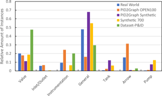
Figure S1: Symbol class distribution: Frequency of symbol object classes among the datasets, showing relative abundance of each class type.

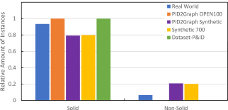
Figure S2: Edge Class Distribution: Relative frequency of each edge class across the datasets.

S3.2 Dataset Structure

For each P&ID, we provide an annotation file in the .graphml-Format. The nodes and edges have attributes that are their bounding boxes and classes. The dataset is structured as shown in Fig. S3.

for tree= font=, grow’=0, child anchor=west, parent anchor=south, anchor=west, calign=first, s sep’=0.9em, edge path= [draw, edge] (!u.south west) +(7.5pt,0) |- node[fill,inner sep=1.25pt] (.child anchor)edge label; , before typesetting nodes= if n=1 insert before=[,phantom] , fit=band, before computing xy=l=15pt, [PID2Graph/ [Complete/ [PID2Graph Synthetic/ [0.png ] [0.graphml ] [… ] ] [PID2Graph OPEN100/ [0.png ] [0.graphml ] [… ] ] ] [Patched/ [PID2Graph Synthetic/ [0/ [0.png ] [0.graphml ] [… ] ] [… ] ] [PID2Graph OPEN100/ [0/ [0.png ] [0.graphml ] [… ] ] [… ] ] ] ]

Figure S3: Structure of the dataset with images and folders.

In Fig. S4, we provide an excerpt of ground truth annotations for a single OPEN100 plan, highlighting the manually drawn bounding boxes that enclose symbols and edges connecting node centers. The latter are computed from the respective box centroids.

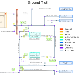
Figure S4: Segment of an annotated diagram from the OPEN100 data, showcasing manually annotated bounding boxes and edges. The annotation represents the ground truth used for evaluation purposes.

S4 Further Analysis of General Class

The confusion matrix of the Relationformer on the PID2Graph OPEN100 dataset is shown in Fig. 5, while the confusion matrices of the Relationformer on the PID2Graph Synthetic and Dataset-P&ID are shown in Fig. S5.

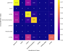
(a)

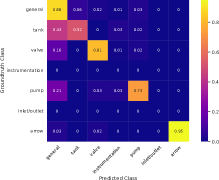
(b)

Figure S5: Confusion matrices for stitched symbol detection results of the Relationformer for (a) Dataset-P&ID and (b) PID2Graph Synthetic.

The confusion is the highest with the ’general’ class for PID2Graph and Dataset-P&ID, with confusion ranging up to 43%.

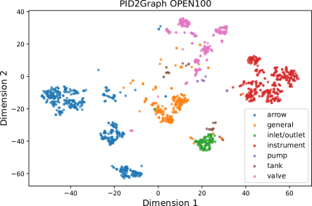
(a)

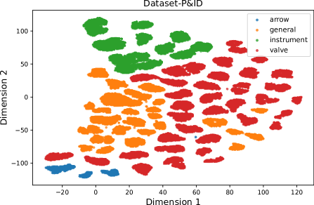
(b)

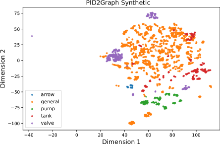
(c)

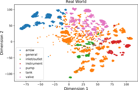
(d)

Figure S6: 2D t-SNE visualization of features by class for (a) PID2Graph OPEN100, (b) Dataset-P&ID, (c) PID2Graph Synthetic and (d) Real World.

To gain deeper insight into the diversity within each class, we extracted feature vectors from every symbol in our dataset using ResNet-101 with an input size of (224, 224). We then applied t-SNE to visualize these features in a 2D space (see Fig. S6). This analysis reveals that the ’general’ class exhibits the highest degree of centralization and overlap with other classes across all datasets. This also suggests substantial intra-class variability for the ’general’ category.

S5 Dataset-P&ID Comparison

The line detection precision of DigitizePID is not directly comparable to edge mAP, however we display both of them.

Our evaluation methods required converting the Dataset-P&ID [26] data into a graph structure (as described in Section 3.4). Notably, we used an Intersection-over-Union (IoU) threshold of 75% for calculating mAP values, which is higher than the 50% threshold used in our other experiments. The line detection precision of DigitizePID is not directly comparable to our edge mAP results, but both metrics are presented for reference.

Table S5: Performance comparison of the Modular Digitization, the Relationformer and DigitizePID on the synthetic Dataset-P&ID dataset.

Dataset-P&ID [26], Stitched
	Symbols	Nodes	Edges	Lines
	mAP	AP	mAP	Accuracy
Modular Digit.	69.82	85.42	85.46	-
Relationformer	43.04	75.85	95.07	-
DigitizePID [26]	92.50	-	-	91.13

Despite this, the results show that both Modular Digitization and Relationformer perform poorly compared to DigitizePID, likely due to differences in IoU thresholds and bounding box styles. Specifically, the loose-fitting bounding boxes in Dataset-P&ID, combined with smaller symbol sizes (cf. Sec. S3.1), resulted in non-detections at this higher IoU. However, our results indicate that the Relationformer’s edge detection is robust and effective.

S6 Additional Examples

We show additional prediction examples for both the Relationformer and Modular Digitization Approach on the OPEN100 data (Figs. S7 and S8) and on the synthetic data (Figs. S9 and S10).

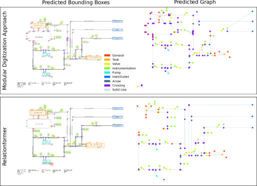
Figure S7: Comparison of digitization results obtained using the Modular Digitization Approach (top) versus the Relationformer (bottom) on an exemplary P&ID from the OPEN100 dataset. Note that this plan is excluded from the small symbol subset and it can be seen that the big tank in the upper left has not been detected correctly by either approach.

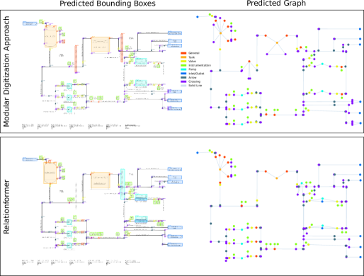
Figure S8: Another comparison of digitization results obtained using the Modular Digitization Approach (top) versus the Relationformer (bottom) on an different P&ID from the OPEN100 dataset.

Figure S9: Comparison of digitization results obtained using the Modular Digitization Approach (top) versus the Relationformer (bottom) on a P&ID from the synthetic ISO10628 dataset.

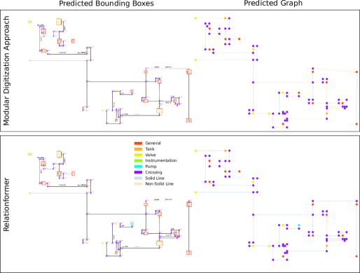
Figure S10: Comparison of digitization results obtained using the Modular Digitization Approach (top) versus the Relationformer (bottom) on a P&ID from the synthetic ISO10628 dataset.

References

- Baek et al. [2019] Youngmin Baek, Bado Lee, Dongyoon Han, Sangdoo Yun, and Hwalsuk Lee. Character region awareness for text detection, 2019.
- Bayer et al. [2023] Johannes Bayer, Amit Kumar Roy, and Andreas Dengel. Instance segmentation based graph extraction for handwritten circuit diagram images, 2023.
- Belli and Kipf [2019] Davide Belli and Thomas Kipf. Image-conditioned graph generation for road network extraction, 2019.
- Bhanbhro et al. [2023] Hina Bhanbhro, Yew Kwang Hooi, Worapan Kusakunniran, and Zaira Hassan Amur. A symbol recognition system for single-line diagrams developed using a deep-learning approach. Applied Sciences, 13(15):8816, 2023.
- Biagioni and Eriksson [2012] James Biagioni and Jakob Eriksson. Inferring road maps from global positioning system traces. Transportation Research Record: Journal of the Transportation Research Board, 2291(1):61–71, 2012.
- Bickel et al. [2024] Sebastian Bickel, Stefan Goetz, and Sandro Wartzack. Symbol detection in mechanical engineering sketches: Experimental study on principle sketches with synthetic data generation and deep learning. Applied Sciences, 14(14):6106, 2024.
- Cha et al. [2019] Jae-Min Cha, Kim Taewoo, Taekyong Lee, and Duhwan Mun. Features recognition from piping and instrumentation diagrams in image format using a deep learning network. Energies, 12(23):4425, 2019.
- Elyan et al. [2020] Eyad Elyan, Laura Jamieson, and Adamu Ali-Gombe. Deep learning for symbols detection and classification in engineering drawings. Neural networks : the official journal of the International Neural Network Society, 129:91–102, 2020.
- Gada [2021] Mihir Gada. Object detection for p&id images using various deep learning techniques. In 2021 International Conference on Computer Communication and Informatics (ICCCI), pages 1–5. IEEE, 2021.
- He et al. [2020] Songtao He, Favyen Bastani, Satvat Jagwani, Mohammad Alizadeh, Hari Balakrishnan, Sanjay Chawla, Mohamed M. Elshrif, Samuel Madden, and Mohammad Amin Sadeghi. Sat2graph: Road graph extraction through graph-tensor encoding. In Computer Vision – ECCV 2020, pages 51–67. Springer International Publishing and Imprint Springer, Cham, 2020.
- ISO Central Secretary [2012] ISO Central Secretary. Diagrams for the chemical and petrochemical industry — Part 2: Graphical symbols. Standard, International Organization for Standardization, 2012.
- JadedAI [2023] JadedAI. Easyocr, 2023.
- Jamieson et al. [2024a] Laura Jamieson, Carlos Francisco Moreno-García, and Eyad Elyan. A review of deep learning methods for digitisation of complex documents and engineering diagrams. Artificial Intelligence Review, 57(6), 2024a.
- Jamieson et al. [2024b] Laura Jamieson, Carlos Francisco Moreno-Garcia, and Eyad Elyan. Towards fully automated processing and analysis of construction diagrams: Ai-powered symbol detection. International Journal on Document Analysis and Recognition (IJDAR), 2024b.
- Kim et al. [2022] Byung Chul Kim, Hyungki Kim, Yoochan Moon, Gwang Lee, and Duhwan Mun. End-to-end digitization of image format piping and instrumentation diagrams at an industrially applicable level. Journal of Computational Design and Engineering, 2022.
- Kim and Kim [2023] Gwangsik Kim and Byung Chul Kim. Classification of functional types of lines in p&ids using a graph neural network. IEEE Access, 11:73680–73687, 2023.
- Kuhn [1955] H. W. Kuhn. The hungarian method for the assignment problem. Naval Research Logistics Quarterly, 2(1-2):83–97, 1955.
- Li et al. [2024] Rongjie Li, Songyang Zhang, and Xuming He. Sgtr+: End-to-end scene graph generation with transformer, 2024.
- Li et al. [2022] Xingchen Li, Long Chen, Jian Shao, Shaoning Xiao, Songyang Zhang, and Jun Xiao. Rethinking the evaluation of unbiased scene graph generation. In 33rd British Machine Vision Conference 2022, BMVC 2022, London, UK, November 21-24, 2022. BMVA Press, 2022.
- Li et al. [2021] Yanghao Li, Saining Xie, Xinlei Chen, Piotr Dollar, Kaiming He, and Ross Girshick. Benchmarking detection transfer learning with vision transformers, 2021.
- Mani et al. [2020] Shouvik Mani, Michael A. Haddad, Dan Constantini, Willy Douhard, Qiwei Li, and Louis Poirier. Automatic digitization of engineering diagrams using deep learning and graph search. In 2020 IEEE/CVF Conference on Computer Vision and Pattern Recognition Workshops (CVPRW), pages 673–679. IEEE, 2020.
- Moreno-Garcia et al. [2020] Carlos Francisco Moreno-Garcia, Pam Johnston, and Bello Garkuwa. Pixel-based layer segmentation of complex engineering drawings using convolutional neural networks. In 2020 International Joint Conference on Neural Networks (IJCNN), pages 1–7. IEEE, 2020.
- Nurminen et al. [2020] Jukka K. Nurminen, Kari Rainio, Jukka-Pekka Numminen, Timo Syrjänen, Niklas Paganus, and Karri Honkoila. Object detection in design diagrams with machine learning. In Progress in Computer Recognition Systems, pages 27–36. Springer International Publishing, Cham, 2020.
- Open100 [30.08.2024] Energy Impact Center Open100. Open100 — nuclear energy. https://www.open-100.com/, 30.08.2024.
- Paganus et al. [2018] Niklas Paganus, Marko Luukkainen, Karri Honkoila, and Tommi Karhela. Automatic generation of dynamic simulation models based on standard engineering data. In Proceedings of The 9th EUROSIM Congress on Modelling and Simulation, EUROSIM 2016, pages 776–782. Linköping University Electronic Press, 2018.
- Paliwal et al. [2021a] Shubham Paliwal, Arushi Jain, Monika Sharma, and Lovekesh Vig. Digitize-pid: Automatic digitization of piping and instrumentation diagrams. In Trends and Applications in Knowledge Discovery and Data Mining, pages 168–180, Cham, 2021a. Springer International Publishing.
- Paliwal et al. [2021b] Shubham Paliwal, Monika Sharma, and Lovekesh Vig. Ossr-pid: One-shot symbol recognition in p&id sheets using path sampling and gcn. International Joint Conference on Neural Network (IJCNN), 2021b.
- Pedregosa et al. [2011] F. Pedregosa, G. Varoquaux, A. Gramfort, V. Michel, B. Thirion, O. Grisel, M. Blondel, P. Prettenhofer, R. Weiss, V. Dubourg, J. Vanderplas, A. Passos, D. Cournapeau, M. Brucher, M. Perrot, and E. Duchesnay. Scikit-learn: Machine learning in Python. Journal of Machine Learning Research, 12:2825–2830, 2011.
- Rahul et al. [2019] Rohit Rahul, Shubham Paliwal, Monika Sharma, and Lovekesh Vig. Automatic information extraction from piping and instrumentation diagrams. In 8th International Conference on Pattern Recognition Applications and Methods, 2019.
- Sandoval [2023] Steven Baltakatei Sandoval. Baltakatei engineering drawing templates. https://gitlab.com/baltakatei/BK-2020-04, 2023. This work is licensed under the Creative Commons Attribution 4.0 International License. To view a copy of this license, visit http://creativecommons.org/licenses/by/4.0/.
- Shit et al. [2022] Suprosanna Shit, Rajat Koner, Bastian Wittmann, Johannes Paetzold, Ivan Ezhov, Hongwei Li, Jiazhen Pan, Sahand Sharifzadeh, Georgios Kaissis, Volker Tresp, and Bjoern Menze. Relationformer: A unified framework for image-to-graph generation. In Computer Vision – ECCV 2022, pages 422–439. Springer Nature Switzerland and Imprint Springer, Cham, 2022.
- Stürmer et al. [12/15/2023 - 12/17/2023] Jan Marius Stürmer, Marius Graumann, and Tobias Koch. Demonstrating automated generation of simulation models from engineering diagrams. In 2023 International Conference on Machine Learning and Applications (ICMLA), pages 1156–1162. IEEE, 12/15/2023 - 12/17/2023.
- Theisen et al. [2023] Maximilian F. Theisen, Kenji Nishizaki Flores, Lukas Schulze Balhorn, and Artur M. Schweidtmann. Digitization of chemical process flow diagrams using deep convolutional neural networks. Digital Chemical Engineering, 6:100072, 2023.
- Toghraei [2019] Moe Toghraei. Piping and instrumentation diagram development. John Wiley & Sons Inc, Hoboken, NJ, USA, first edition edition, 2019.
- van Etten et al. [2018] Adam van Etten, Dave Lindenbaum, and Todd M. Bacastow. Spacenet: A remote sensing dataset and challenge series, 2018.
- Xia et al. [2024] Liegang Xia, Ruiyan Liu, Yishao Su, Shulin Mi, Dezhi Yang, Jun Chen, and Zhanfeng Shen. Crop field extraction from high resolution remote sensing images based on semantic edges and spatial structure map. Geocarto International, 39(1), 2024.
- Yang et al. [2024] Lvyang Yang, Jiankang Zhang, Huaiqiang Li, Longfei Ren, Chen Yang, Jingyu Wang, and Dongyuan Shi. A comprehensive end-to-end computer vision framework for restoration and recognition of low-quality engineering drawings. Engineering Applications of Artificial Intelligence, 133:108524, 2024.
- Zhu et al. [2022] Guangming Zhu, Liang Zhang, Youliang Jiang, Yixuan Dang, Haoran Hou, Peiyi Shen, Mingtao Feng, Xia Zhao, Qiguang Miao, Syed Afaq Ali Shah, and Mohammed Bennamoun. Scene graph generation: A comprehensive survey, 2022.
- Zhu et al. [2020] Xizhou Zhu, Weijie Su, Lewei Lu, Bin Li, Xiaogang Wang, and Jifeng Dai. Deformable detr: Deformable transformers for end-to-end object detection, 2020.