Rational Ruijsenaars–Schneider model

with cosmological constant

Anton Galajinsky  
Tomsk Polytechnic University, 634050 Tomsk, Lenin Ave. 30, Russia

Tomsk State University of Control Systems and Radioelectronics,
Lenin ave. 40, 634050 Tomsk, Russia

e-mail: galajin@tpu.ru

The Ruijsenaars–Schneider models are integrable dynamical realizations of the Poincaré group in $1+1$ dimensions, which reduce to the Calogero and Sutherland systems in the nonrelativistic limit. In this work, a possibility to construct a one–parameter deformation of the Ruijsenaars–Schneider models by uplifting the Poincaré algebra in $1+1$ dimensions to the anti de Sitter algebra is studied. It is shown that amendments including a cosmological constant are feasible for the rational variant, while the hyperbolic and trigonometric systems are ruled out by our analysis. The issue of integrability of the deformed rational model is discussed in some detail. A complete proof of integrability remains a challenge.

Keywords: Ruijsenaars-Schneider models, anti de Sitter algebra, cosmological constant

1. Introduction

The Ruijsenaars-Schneider models [1, 2] comprise interesting examples of integrable many–body systems, equations of motion of which involve particle velocities. They furnish dynamical realizations of the Poincaré group in $1+1$ dimensions, which includes translations in temporal and spatial directions and the Lorentz boost, and reduce to the celebrated Calogero and Sutherland models [3, 4] in the nonrelativistic limit. By this reason, the former are conventionally regarded as relativistic generalizations of the latter. The relativistic systems of such a type proved relevant for various physical applications including dualities (for a review and further references see [5]).

As is well known, the Poincaré algebra can be regarded as a contraction of the (anti) de Sitter algebra in which a cosmological constant tends to zero [6]. A natural question arises whether the analysis in [1] can be extended so as to include a cosmological constant.

The goal of this work is to study a possibility to construct a one–parameter deformation of the Ruijsenaars–Schneider models by uplifting the Poincaré algebra in $1+1$ dimensions to the anti de Sitter algebra. As shown below, amendments including a cosmological constant are feasible for the rational variant, while the hyperbolic and trigonometric systems are ruled out by our analysis.

The work is organized as follows. In the next section, the original construction in [1] is briefly reviewed.

In Sect. 3, starting with the anti de Sitter algebra, which is a one–parameter deformation of the Poincaré algebra in $1+1$ dimensions, and properly modifying the generators which furnish a dynamical realization, two functional equations are obtained, which determine interaction potential. The first equation coincides with that in [1]. The second restriction is shown to be compatible with the rational model but it rules out the trigonometric and hyperbolic variants. Because the anti de Sitter algebra in $1+1$ dimensions is isomorphic to the conformal algebra $so(2,1)$, the generalized rational model in this work provides a new dynamical realization of the conformal group $SO(2,1)$ within the framework of many–body mechanics in one dimension.

In Sect. 4, equations of motion of the rational Ruijsenaars–Schneider model with a cosmological constant are constructed. The derivation relies upon specific subsidiary functions, which via the Poisson bracket generate interaction potential of interest. Similar formalism has previously proved useful for constructing supersymmetric extensions [7]. Like in the nonrelativistic case [8], the presence of a cosmological constant results in an effective confining potential which renders particles motion (quasi)periodic.

The issue of integrability is discussed in Sect. 5. Constants of motion characterizing the three–body case are explicitly constructed.

We summarize our results and discuss possible further developments in the concluding Sect. 6.

Throughout the paper, summation signs are written out explicitly, i.e. no summation over repeated indices is understood.

2. The Ruijsenaars–Schneider models

The Ruijsenaars–Schneider models were originally introduced in [1] as dynamical realizations of the Poincaré group in $1+1$ dimensions (for a review see [2]). The key feature of the construction is that the angle $\varphi$ which specifies the Lorentz transformation in two–dimensional spacetime

$$\left(\begin{array}[]{cccc}ct^{\prime}\\ x^{\prime}\\ \end{array}\right)=\left(\begin{array}[]{cccc}\cosh{\varphi}&\sinh{\varphi}\\ \vspace{0.2cm}\sinh{\varphi}&\cosh{\varphi}\\ \end{array}\right)\left(\begin{array}[]{cccc}ct\\ x\\ \end{array}\right)$$ (1)

is represented as the ratio of the rapidity $\theta$ and the speed of light $c$

$$\varphi=\frac{\theta}{c}$$ (2)

and $\theta$ is taken to be a dynamical variable instead of the velocity $v$ used within the special relativity.

The well known relation

$$\tanh{\frac{\theta}{c}}=-\frac{v}{c}$$

links (1) to the conventional form of the Lorentz boost

$$t^{\prime}=\frac{t-\frac{v}{c^{2}}x}{\sqrt{1-{\left(\frac{v}{c}\right)}^{2}}},\qquad x^{\prime}=\frac{x-vt}{\sqrt{1-{\left(\frac{v}{c}\right)}^{2}}},$$ (3)

as well as yields

$$H=\frac{mc^{2}}{\sqrt{1-{\left(\frac{v}{c}\right)}^{2}}}=mc^{2}\cosh{\frac{\theta}{c}}$$ (4)

for the energy of a free relativistic particle. The rightmost expression in (4) is the Ruijsenaars–Schneider Hamiltonian for a single relativistic particle moving on a real line. Particle’s momentum $P$ is found from the relativistic mass–shell condition

$${\left(\frac{H}{c}\right)}^{2}-P^{2}=m^{2}c^{2}\quad\rightarrow\quad P=mc\sinh{\frac{\theta}{c}}.$$ (5)

In order to construct a many–body interacting generalization, one invokes the symmetry argument. Considering $\theta$ in (1), (2) to be an infinitesimal parameter

$$t^{\prime}=t+\frac{\theta}{c^{2}}x,\qquad x^{\prime}=x+\theta t,$$

one finds the generator of the Lorentz transformation $K=\frac{1}{c^{2}}x\partial_{t}+t\partial_{x}$ which jointly with the generators of the temporal and spatial translations $H=\partial_{t}$ and $P=\partial_{x}$ obeys the structure relations of the Poincaré algebra in two spacetime dimensions

$$[H,P]=0, [H,K]=P, [P,K]=\frac{1}{c^{2}}H.$$ (6)

Eqs. (4), (5) and (6) underlie the Ruijsenaars–Schneider construction [1, 2] which is implemented within the Hamiltonian framework. Firstly, one notices that the functions

$$H=mc^{2}\sum_{i=1}^{N}\cosh{\left(\frac{p_{i}}{mc}\right)}, P=mc\sum_{i=1}^{N}\sinh{\left(\frac{p_{i}}{mc}\right)}, K=-m\sum_{i=1}^{N}x_{i}$$ (7)

defined on a phase space parametrized by the canonical pairs $(x_{i},p_{i})$, $i=1,\dots,N$, obey the algebra (6) under the conventional Poisson bracket $\{x_{i},p_{j}\}=\delta_{ij}$. Then one alters the first two expressions in (7) by introducing the interaction potential

$$H=mc^{2}\sum_{i=1}^{N}\cosh{\left(\frac{p_{i}}{mc}\right)}\prod_{k\neq i}f(x_{i}-x_{k}),\quad P=mc\sum_{i=1}^{N}\sinh{\left(\frac{p_{i}}{mc}\right)}\prod_{k\neq i}f(x_{i}-x_{k}),$$ (8)

with $f(x)$ to be fixed below, keeps $K$ intact, and finally demands the structure relations (6) to be satisfied under the Poisson bracket. The brackets involving $K$ hold automatically, while $\{H,P\}=0$ forces one to assume that $f(x)$ is an even function of its argument which additionally obeys the functional equation [1]

$$\sum_{i=1}^{N}\partial_{i}\prod_{j\neq i}f^{2}(x_{i}-x_{j})=0,$$ (9)

where $\partial_{i}=\frac{\partial}{\partial x_{i}}$.

Taking into account the nonrelativistic limit

$$\lim_{c\to\infty}(H_{rel}-mc^{2}N)=H_{nr},$$

and appealing to earlier results by Calogero [3] and Sutherland [4] on integrable nonrelativistic many–body systems, one can construct three explicit solutions to the functional equation (9)

$$f_{r}(x)={\left(1+\frac{g^{2}}{m^{2}c^{2}x^{2}}\right)}^{\frac{1}{2}},\qquad f_{tr}(x)={\left(1+\frac{\sinh^{2}{\left(\frac{\nu g}{mc}\right)}}{\sin^{2}{\left(\nu x\right)}}\right)}^{\frac{1}{2}},$$ (10)

$$f_{h}(x)={\left(1+\frac{\sin^{2}{\left(\frac{\nu g}{mc}\right)}}{\sinh^{2}{\left(\nu x\right)}}\right)}^{\frac{1}{2}},$$

where $g$ and $\nu$ are arbitrary real parameters. They give rise to what is nowadays known as the rational, trigonometric, and hyperbolic Ruijsenaars–Schneider models [1].

3. Rational Ruijsenaars–Schneider model with cosmological constant

As is well known, the Poincaré algebra (6) can be viewed as a contraction of the (anti) de Sitter algebra

$$[H,P]=\pm\frac{1}{R^{2}}K, [H,K]=P, [P,K]=\frac{1}{c^{2}}H,$$ (11)

in which the characteristic time $R$ goes to infinity [6]. In physics literature, $\pm\frac{1}{c^{2}R^{2}}$ is identified with the cosmological constant. Our objective in this section is to study a possibility to deform the Ruijsenaars–Schneider models above so as to include a cosmological constant. For physical reasons (see Eq. (16) below), we focus on the anti de Sitter algebra (negative cosmological constant), which corresponds to the lower sign in $[H,P]$ above.

A natural starting point is to alter a free particle realization of the Poincaré algebra in the preceding section

$$H=mc^{2}F(x)\cosh{\frac{p}{mc}},\qquad P=mcF(x)\sinh{\frac{p}{mc}},\qquad K=-mx,$$ (12)

where $(x,p)$ is a canonical pair obeying the Poisson bracket $\{x,p\}=1$, and $F(x)$ is a function to be fixed below. Demanding the structure relations (11) to hold under the Poisson bracket, one finds the differential equation to fix $F(x)$

$$c^{2}R^{2}F(x)F^{\prime}(x)-x=0,\qquad\rightarrow\qquad F(x)=\pm\sqrt{\alpha+\frac{x^{2}}{c^{2}R^{2}}},$$ (13)

where $\alpha$ is a constant of integration.

Because the nonrelativistic limit of the (anti) de Sitter algebra results in the Newton–Hooke algebra [6], consistency requires the nonrelativistic limit of the Hamiltonian $H$ in (12) to reproduce that of a particle moving in the Newton–Hooke spacetime [8]

$$\lim_{c\to\infty}(H-mc^{2})=\frac{1}{2m}p^{2}+\frac{m}{2R^{2}}x^{2},$$ (14)

where the latter term describes the universal cosmological attraction within the nonrelativistic framework. Eq. (14) determines the form of the factor $F(x)$ entering (12)

$$F(x)=\sqrt{1+\frac{x^{2}}{c^{2}R^{2}}}.$$ (15)

Note that, had one started with the de Sitter algebra involving $[H,P]=\frac{1}{R^{2}}K$ (positive cosmological constant), one would have obtained an unstable mechanical system governed by the Hamiltonian

$$H=\frac{1}{2m}p^{2}-\frac{m}{2R^{2}}x^{2}$$ (16)

in the nonrelativistic limit. For physical reasons, this instance should be discarded.

A single–particle pattern above, suggests the way of how to proceed when building an interacting system. One starts with the ansatz

$$H=mc^{2}\sum_{i=1}^{N}\sqrt{1+\frac{x_{i}^{2}}{c^{2}R^{2}}}\cosh{\left(\frac{p_{i}}{mc}\right)}\prod_{k\neq i}f(x_{i}-x_{k}),$$

$$P=mc\sum_{i=1}^{N}\sqrt{1+\frac{x_{i}^{2}}{c^{2}R^{2}}}\sinh{\left(\frac{p_{i}}{mc}\right)}\prod_{k\neq i}f(x_{i}-x_{k}),$$

$$K=-m\sum_{i=1}^{N}x_{i},$$ (17)

where $f(x)$ is assumed to be an even function of its argument, which is independent of the parameter $R$, and requires the structure relations (11) to hold under the Poisson bracket. Like in the preceding section, all restrictions upon the form of $f(x)$ come from the bracket $\{H,P\}=-\frac{1}{R^{2}}K$. Collecting terms without the factor $\frac{1}{R^{2}}$, one reproduces the functional relation (9), while terms involving $\frac{1}{R^{2}}$ yield

$$\sum_{i=1}^{N}\left(2x_{i}-\partial_{i}\left(x_{i}^{2}\prod_{j\neq i}f^{2}(x_{i}-x_{j})\right)\right)=0.$$ (18)

Because the restriction (9) continues to hold, three prepotentials (10) can be checked against the additional condition (18), which is a consequence of the presence of a cosmological constant in the Lie algebra structure relations (11). It is straightforward to verify that only the rational model passes the hurdle.

Focusing on the rational model and analyzing the nonrelativisit limit $\lim_{c\to\infty}(H_{rel}-mc^{2}N)=H_{nr}$, one reproduces the Calogero model in the harmonic trap

$$H_{nr}=\frac{1}{2m}\sum_{i=1}^{N}p_{i}^{2}+\sum_{i<j}^{N}\frac{g^{2}}{m{(x_{i}-x_{j})}^{2}}+\frac{m}{2R^{2}}\sum_{i=1}^{N}x_{i}^{2}.$$ (19)

Within the nonrelativistic framework, the latter term correctly represents the universal cosmological attraction [8].

To summarize, eqs. (S0.Ex5), in which $f(x)=f_{r}(x)$ and $f_{r}(x)$ is given in (10), determine a one–parameter deformation of the rational Ruijsenaars–Schneider system originating from the anti de Sitter algebra (11). Because the latter is isomorphic to the conformal algebra $so(2,1)$, eqs. (S0.Ex5) can alternatively be viewed as providing a new dynamical realization of the conformal group $SO(2,1)$ within the framework of many–body mechanics in one dimension.

4. Equations of motion

It is interesting to inquire how the presence of the cosmological constant affects the original equations of motion and particle dynamics. To this end, it proves convenient to represent the Hamiltonian in (S0.Ex5) in the manifestly positive–definite form

$$H=\sum_{i=1}^{N}\left(\lambda^{+}_{i}\lambda^{+}_{i}+\lambda^{-}_{i}\lambda^{-}_{i}\right),$$ (20)

where

$$\lambda^{\pm}_{i}={\left(\frac{mc^{2}}{2}e^{\pm\frac{p_{i}}{mc}}\sqrt{1+\frac{x_{i}^{2}}{c^{2}R^{2}}}\prod_{k\neq i}f_{r}(x_{i}-x_{k})\right)}^{\frac{1}{2}},$$ (21)

with $f_{r}(x)$ in (10), and then compute the algebra of the subsidiary functions $\lambda^{\pm}_{i}$

$$\{\lambda^{+}_{i},\lambda^{+}_{j}\}=\frac{1}{2}W(x_{i}-x_{j})\lambda^{+}_{i}\lambda^{+}_{j},\qquad\{\lambda^{-}_{i},\lambda^{-}_{j}\}=-\frac{1}{2}W(x_{i}-x_{j})\lambda^{-}_{i}\lambda^{-}_{j},$$

$$\{\lambda^{+}_{i},\lambda^{-}_{j}\}=-\frac{1}{2}\lambda^{+}_{i}\lambda^{-}_{i}\left(\frac{1}{mc\left(1+\frac{x_{i}^{2}}{c^{2}R^{2}}\right)}\frac{x_{i}}{c^{2}R^{2}}-\sum_{k\neq i}W(x_{i}-x_{k})\right)\delta_{ij}$$ (22)

where $\delta_{ij}$ is the Kronecker delta and $W(x_{i}-x_{j})$ reads

$$W(x_{i}-x_{j})=\left\{\begin{aligned} 0\qquad\qquad,&\qquad i=j\\ \frac{1}{mc\left(x_{i}-x_{j}\right)\left(1+\frac{{(mc)}^{2}{\left(x_{i}-x_{j}\right)}^{2}}{g^{2}}\right)},&\qquad i\neq j\\ \end{aligned}\right.$$ (23)

Note that $W(x)$ is independent of the cosmological constant.

Taking into account the Poisson brackets

$$\{x_{i},\lambda^{\pm}_{j}\}=\pm\frac{1}{2mc}\lambda^{\pm}_{j}\delta_{ij},$$ (24)

one can easily obtain the Hamiltonian equations of motion which govern the evolution of $x_{i}$ and $\lambda^{\pm}_{i}$ over time

$${\dot{x}}_{i}=\frac{1}{mc}\left({\left(\lambda^{+}_{i}\right)}^{2}-{\left(\lambda^{-}_{i}\right)}^{2}\right),$$ (25)

$${\dot{\lambda}}^{+}_{i}=\sum_{j\neq i}W(x_{i}-x_{j})\lambda^{+}_{i}{\left(\lambda^{+}_{j}\right)}^{2}-\lambda^{+}_{i}{\left(\lambda^{-}_{i}\right)}^{2}\left(\frac{1}{mc\left(1+\frac{x_{i}^{2}}{c^{2}R^{2}}\right)}\frac{x_{i}}{c^{2}R^{2}}-\sum_{j\neq i}W(x_{i}-x_{j})\right),$$

$${\dot{\lambda}}^{-}_{i}=-\sum_{j\neq i}W(x_{i}-x_{j})\lambda^{-}_{i}{\left(\lambda^{-}_{j}\right)}^{2}+\lambda^{-}_{i}{\left(\lambda^{+}_{i}\right)}^{2}\left(\frac{1}{mc\left(1+\frac{x_{i}^{2}}{c^{2}R^{2}}\right)}\frac{x_{i}}{c^{2}R^{2}}-\sum_{j\neq i}W(x_{i}-x_{j})\right).$$

The first equation in (25) allows one to express momenta $p_{i}$ in terms of $x_{i}$ and ${\dot{x}}_{i}$

$$e^{\pm\frac{p_{i}}{mc}}=\frac{\pm{\dot{x}}_{i}+y_{i}}{c\sqrt{1+\frac{x_{i}^{2}}{c^{2}R^{2}}}\prod_{k\neq i}f_{r}(x_{i}-x_{k})},$$ (26)

where we denoted

$$y_{i}=\sqrt{{\dot{x}}_{i}^{2}+c^{2}\left(1+\frac{x_{i}^{2}}{c^{2}R^{2}}\right)\prod_{k\neq i}f_{r}^{2}(x_{i}-x_{k})},$$ (27)

while differentiating ${\dot{x}}_{i}$ with respect to the temporal variable and taking into account (25) and (26), one obtains the desired equations of motion

$${\ddot{x}}_{i}=mc\sum_{j\neq i}W(x_{i}-x_{j})\left({\dot{x}}_{i}{\dot{x}}_{j}+y_{i}y_{j}\right)$$

$$\quad\quad-\left(\frac{x_{i}}{R^{2}}-mc^{3}\left(1+\frac{x_{i}^{2}}{c^{2}R^{2}}\right)\sum_{j\neq i}W(x_{i}-x_{j})\right)\prod_{k\neq i}f_{r}^{2}(x_{i}-x_{k}),$$ (28)

with $y_{i}$ given in (27). The terms involving $\frac{1}{R^{2}}$ comprise the difference with the original rational Ruijsenaars–Schneider model.

A qualitative difference in particle dynamics is illustrated in Fig. 1 and Fig. 2. The former depicts a numerical solution of the equations of motion of the three–body model with vanishing cosmological constant for a particular choice of the free parameters $m=c=g=1$ and initial conditions $x_{1}(0)=1$, ${\dot{x}}_{1}(0)=0.1$ (blue), $x_{2}(0)=2$, ${\dot{x}}_{2}(0)=0.2$ (orange), $x_{3}(0)=3$, ${\dot{x}}_{3}(0)=0.3$ (green) on the time interval $t\in[0,10^{6}]$. The latter displays solutions of (S0.Ex10) with $R=10^{5}$ for the same choise of the free parameters, initial conditions, and time interval. As is seen from the graphs, in the former case the motion is unbounded, while in the latter case the particles move along (quasi)periodic orbits.

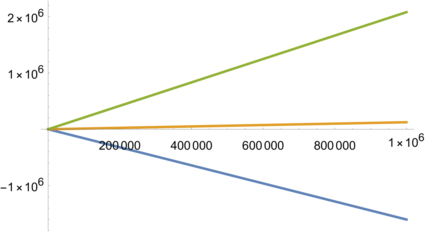
Figure 1: The graph of $x_{i}$ versus $t$ for the three–body rational Ruijsenaars–Schneider system with $m=c=g=1$, $x_{1}(0)=1$, ${\dot{x}}_{1}(0)=0.1$ (blue), $x_{2}(0)=2$, ${\dot{x}}_{2}(0)=0.2$ (orange), $x_{3}(0)=3$, ${\dot{x}}_{3}(0)=0.3$ (green) and $t\in[0,10^{6}]$.

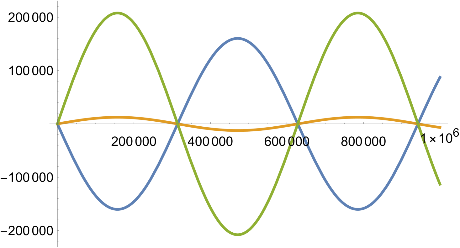
Figure 2: The graph of $x_{i}$ versus $t$ for the three–body rational Ruijsenaars–Schneider system with the cosmological constant derived from $R=10^{5}$, and $m=c=g=1$, $x_{1}(0)=1$, ${\dot{x}}_{1}(0)=0.1$ (blue), $x_{2}(0)=2$, ${\dot{x}}_{2}(0)=0.2$ (orange), $x_{3}(0)=3$, ${\dot{x}}_{3}(0)=0.3$ (green), $t\in[0,10^{6}]$.

Eqs. (S0.Ex10) reduce to

$${\ddot{x}}_{i}=\sum_{j\neq i}\frac{2g^{2}}{m^{2}{\left(x_{i}-x_{j}\right)}^{3}}-\frac{x_{i}}{R^{2}}$$ (29)

in the nonrelativistic limit $c\to\infty$, which correctly reproduce the Lagrangian equations of motion associated with the Calogero model in the harmonic trap (19). Within the nonrelativistic framework, the Hooke’s term $-\frac{x_{i}}{R^{2}}$ describes the universal cosmological attraction [8]. As is seen in (S0.Ex10), its relativistic analogue is realized in a rather more fanciful way.

A salient feature of the Ruijsenaars–Schneider systems is that they are integrable. As explained in [1, 2], the integrability is maintained if one considers reduced models governed by either $H^{+}=\sum_{i=1}^{N}\lambda^{+}_{i}\lambda^{+}_{i}$ or $H^{-}=\sum_{i=1}^{N}\lambda^{-}_{i}\lambda^{-}_{i}$. In each case, the canonical equations of motion

$${\dot{x}}_{i}=\pm\frac{1}{mc}{\left(\lambda^{\pm}_{i}\right)}^{2},\qquad{\dot{\lambda}}^{\pm}_{i}=\pm\sum_{j\neq i}W(x_{i}-x_{j})\lambda^{\pm}_{i}{\left(\lambda^{\pm}_{j}\right)}^{2}$$ (30)

can be rewritten in the geodesic form

$${\ddot{x}}_{i}=2mc\sum_{j\neq i}W(x_{i}-x_{j}){\dot{x}}_{i}{\dot{x}}_{j},$$ (31)

with $W(x_{i}-x_{j})$ exposed in (23). Note that ${\dot{x}}_{i}>0$ for the dynamical system governed by $H^{+}$ meaning that particles are moving from left to right (right moving modes). For the model determined by $H^{-}$, they move in the opposite direction (left moving modes).

Although such models degenerate to free dynamics ${\ddot{x}}_{i}=0$ in the nonrelativistic limit, they have been extensively studied in the past. Most notably, the corresponding equations of motion can be put into the Lax form [3]. As follows from $W(x_{i}-x_{j})$ in (23), the explicit dependence on the cosmological constant is absent for the reduced systems, which correlates with the fact that in each respective case one has modes of one and the same type only, their relative motion being insensible to the universal cosmological attraction.

5. The issue of integrability

A salient feature of the Ruijsenaars–Schneider systems is that they are integrable. This is usually demonstrated by considering the Poisson–commuting set of functions [1]

$$S^{+}_{1}=\sum_{i=1}^{N}e^{\frac{p_{i}}{mc}}\prod_{j\neq i}f(x_{i}-x_{j}),$$ (32)

$$S^{+}_{2}=\sum_{i<j}^{N}e^{\frac{p_{i}}{mc}+\frac{p_{j}}{mc}}\prod_{k\neq i,j}f(x_{i}-x_{k})f(x_{j}-x_{k}),$$

$$S^{+}_{3}=\sum_{i<j<k}^{N}e^{\frac{p_{i}}{mc}+\frac{p_{j}}{mc}+\frac{p_{k}}{mc}}\prod_{l\neq i,j,k}f(x_{i}-x_{l})f(x_{j}-x_{l})f(x_{k}-x_{l}),$$

$$\dots$$

where $\dots$ designate higher order invariants of similar structure, verifying that $S^{-}_{i}$, $i=1,\dots,N$, which follow from $S^{+}_{i}$ by reversing the sign of each $p_{i}$, can be algebraically built from $S^{+}_{i}$: $S^{-}_{i}=S^{+}_{N-i}/S^{+}_{N}$, with $S^{+}_{0}=1$, and finally observing that the Hamiltonian in (8) is a linear combination of $S^{+}_{1}$ and $S^{-}_{1}$.

Because $S^{+}_{i}$ commute under the Poisson bracket, any member of the set can be chosen to define a Hamiltonian of an integrable system of the Ruijsenaars–Schneider type. In particular, the Hamiltonians $S^{\pm}_{1}$ govern the dynamics of the right/left movers discussed in the preceding section.

Introducing subsidiary functions similar to $\lambda^{+}_{i}$ in (21)

$$L^{+}_{i}={\left(e^{\frac{p_{i}}{mc}}\prod_{k\neq i}f_{r}(x_{i}-x_{k})\right)}^{\frac{1}{2}},$$ (33)

one can rewrite (32) in the equivalent form

$$S^{+}_{1}=\sum_{i=1}^{N}{\left(L^{+}_{i}\right)}^{2},\qquad S^{+}_{2}=\sum_{i<j}^{N}{\left(L^{+}_{i}\right)}^{2}{\left(L^{+}_{j}\right)}^{2}f^{-2}_{r}(x_{i}-x_{j}),$$

$$S^{+}_{3}=\sum_{i<j<k}^{N}{\left(L^{+}_{i}\right)}^{2}{\left(L^{+}_{j}\right)}^{2}{\left(L^{+}_{k}\right)}^{2}f^{-2}_{r}(x_{i}-x_{j})f^{-2}_{r}(x_{i}-x_{k})f^{-2}_{r}(x_{j}-x_{k}),$$

$$\dots.$$ (34)

In this notation, the fact that the functions Poisson–commute is verified with the use of the relations

$$\{L^{+}_{i},L^{+}_{j}\}=\frac{1}{2}W(x_{i}-x_{j})L^{+}_{i}L^{+}_{j},$$

$$\{L^{+}_{i},f^{-2}_{r}(x_{j}-x_{k})\}=-W(x_{j}-x_{k})f^{-2}_{r}(x_{j}-x_{k})L^{+}_{i}\left(\delta_{ij}-\delta_{ik}\right),$$ (35)

where $W(x_{j}-x_{k})$ is defined in (23) and $\delta_{ij}$ is the Kronecker delta.

If a cosmological constant is present, a natural modification of (32) reads

$$\mathcal{S}^{+}_{1}=\sum_{i=1}^{N}e^{\frac{p_{i}}{mc}}\sqrt{1+\frac{x_{i}^{2}}{c^{2}R^{2}}}\prod_{j\neq i}f_{r}(x_{i}-x_{j}),$$

$$\mathcal{S}^{+}_{2}=\sum_{i<j}^{N}e^{\frac{p_{i}}{mc}+\frac{p_{j}}{mc}}\sqrt{\left(1+\frac{x_{i}^{2}}{c^{2}R^{2}}\right)\left(1+\frac{x_{j}^{2}}{c^{2}R^{2}}\right)}\prod_{k\neq i,j}f_{r}(x_{i}-x_{k})f_{r}(x_{j}-x_{k}),$$

$$\mathcal{S}^{+}_{3}=\sum_{i<j<k}^{N}e^{\frac{p_{i}}{mc}+\frac{p_{j}}{mc}+\frac{p_{k}}{mc}}\sqrt{\left(1+\frac{x_{i}^{2}}{c^{2}R^{2}}\right)\left(1+\frac{x_{j}^{2}}{c^{2}R^{2}}\right)\left(1+\frac{x_{k}^{2}}{c^{2}R^{2}}\right)}$$

$$\qquad\times\prod_{l\neq i,j,k}f_{r}(x_{i}-x_{l})f_{r}(x_{j}-x_{l})f_{r}(x_{k}-x_{l}),$$

$$\dots$$

while $\mathcal{S}^{-}_{i}$ are obtained by reversing the sign of each $p_{i}$. The fact that $\mathcal{S}^{+}_{i}$ form a Poisson–commuting set of functions can be established by deforming $L^{+}_{i}$ in (33) as follows

$$L^{+}_{i}\quad\rightarrow\quad\mathcal{L}^{+}_{i}={\left(e^{\frac{p_{i}}{mc}}\sqrt{1+\frac{x_{i}^{2}}{c^{2}R^{2}}}\prod_{k\neq i}f_{r}(x_{i}-x_{k})\right)}^{\frac{1}{2}},$$ (37)

rewriting $\mathcal{S}^{+}_{i}$ in terms of $\mathcal{L}^{+}_{i}$ like in eqs. (S0.Ex14) above, and finally verifying that $\mathcal{L}^{+}_{i}$ obey the same algebraic relations (S0.Ex16) as the original $L^{+}_{i}$.

In contrast to the flat case, $\mathcal{S}^{-}_{i}$ are no longer expressible in terms of $\mathcal{S}^{+}_{i}$, in particular

$$\{\mathcal{S}^{+}_{1},\mathcal{S}^{-}_{1}\}=-\frac{2}{mc^{3}R^{2}}\sum_{i=1}^{N}x_{i},$$ (38)

which means that the above analysis of integrability should be modified accordingly. Rewriting the Hamiltonian in (S0.Ex5) in terms of $\mathcal{S}^{\pm}_{1}$

$$H=\frac{mc^{2}}{2}\left(\mathcal{S}^{+}_{1}+\mathcal{S}^{-}_{1}\right),$$ (39)

and taking into account the Poisson brackets

$$\{\mathcal{S}^{\pm}_{1},\sum_{i=1}^{n}x_{i}\}=\mp\frac{1}{mc}\mathcal{S}^{\pm}_{1},$$ (40)

one can readily construct a conserved quantity

$$I_{1}=\mathcal{S}^{+}_{1}\mathcal{S}^{-}_{1}-\frac{1}{c^{2}R^{2}}{\left(\sum_{i=1}^{n}x_{i}\right)}^{2},$$ (41)

which links to the Casimir invariant of the anti de Sitter algebra (11).

Because the Hamiltonian (39) is symmetric under the interchange of $\mathcal{S}^{+}_{1}$ and $\mathcal{S}^{-}_{1}$, it seems natural to search for other integrals of motion in the form symmetric under the interchange of $\mathcal{S}^{\pm}_{i}$

$$\mathcal{S}^{+}_{2}+\mathcal{S}^{-}_{2}+\dots,\qquad\mathcal{S}^{+}_{3}+\mathcal{S}^{-}_{3}+\dots,\qquad\mbox{etc.}$$ (42)

where $\dots$ designate extra contributions needed in order to ensure the commutativity with $H$. It appears that the missing contributions can be built in terms of the elementary monomials in $x_{i}$

$$M_{1}=\sum_{i=1}^{N}x_{i},\qquad M_{2}=\sum_{i<j}^{n}x_{i}x_{j},\qquad M_{3}=\sum_{i<j<k}^{n}x_{i}x_{j}x_{k},\qquad\dots$$ (43)

In particular, a direct inspection of the three–body case reveals the following constants of motion

$$I_{2}=\mathcal{S}^{+}_{2}+\mathcal{S}^{-}_{2}+\frac{2}{c^{2}R^{2}}M_{2},\qquad I_{3}=\mathcal{S}^{+}_{3}+\mathcal{S}^{-}_{3}-\frac{m}{cR^{2}}\{\mathcal{S}^{+}_{1},M_{3}\}+\frac{m}{cR^{2}}\{\mathcal{S}^{-}_{1},M_{3}\},$$ (44)

where the last two terms are compactly written in terms of the Poisson brackets.

Curiously enough, the first integrals $I_{1}$, $I_{2}$, and $I_{3}$ do not commute with each other yielding higher order invariants. This means that even more sophisticated analysis is needed in order to establish the Liouville integrability of the model at hand. In the latter regard, it is important to stress that the Lax representation for the equations of motion without a cosmological constant is known in the literature for the right/left movers only [3]. Were it available for the full system governed by the Hamiltonian in (8), an amendment to include the cosmological constant would be rather straightforward. A transparent algebraic scheme enabling one to build Poisson commuting and functionally independent integrals of motion for the system under consideration remains a challenge.

6. Conclusion

To summarize, in this work the original construction of Ruijsenaars and Schneider in [1] was extended so as to include a cosmological constant. Specifically, starting with the anti de Sitter algebra (11), which is a one–parameter deformation of the Poincaré algebra in $1+1$ dimensions, and properly modifying the generators which furnish a dynamical realization, two functional equations were obtained, which determined possible interactions. The first equation coincided with that in [1]. The second restriction proved compatible with the rational model but ruled out the trigonometric and hyperbolic variants. The issue of integrability was discussed in some detail. In particular, constants of motion characterizing the three–body case were explicitly constructed.

Turning to possible further developments, the most intriguing issue is to build a handy algebraic scheme of constructing Poisson–commuting and functionally independent integrals of motion for the system at hand. It appears one has to reconsider the issue of representing the equations of motion of the complete rational Ruijsenaars–Schneider model in flat space (not just the right or left movers) in the Lax form. In the latter regard, a link to reductions of matrix models [5] seems to provide a promising avenue. A matrix model progenitor of the rational Ruijsenaars–Schneider model with a cosmological constant is worth studying as well.

In a series of recent works [7], [9]–[13], supersymmetric extensions of the Ruijsenaars–Schneider models were built and their integrability was studied. It would be interesting to explore whether the analysis in this work is compatible with supersymmetry.

Acknowledgements

This work was supported by the Russian Science Foundation, grant No 23-11-00002.

References

[1]
S. Ruijsenaars, H. Schneider, A new class of integrable systems and its relation to
solitons, Annals Phys. 170 (1986) 370.
[2]
S. Ruijsenaars, Systems of Calogero–Moser type. In: G. Semenoff, L. Vinet L. (eds).
Particles and fields. CRM series in mathematical physics. Springer (1999).
[3]
F. Calogero, Classical many–body problems
amenable to exact treatments, Lecture Notes in Physics: Monographs 66,
Springer, 2001.
[4]
B. Sutherland, Beautiful models: 70 years of exactly solved quantum many-body problems,
World Scientific Publishing Company, 2004.
[5]
V. Fock, A. Gorsky, N. Nekrasov, V. Rubtsov, Duality in integrable systems and gauge theories,
JHEP 07 (2000) 028, hep-th/9906235.
[6]
H. Bacry, J. Levy–Leblond, Possible kinematics, J. Math. Phys. 9 (1968) 1605.
[7]
A. Galajinsky, Ruijsenaars–Schneider three–body models with supersymmetry,
JHEP 04 (2018) 079, arXiv:1802.08011.
[8]
G.W. Gibbons, C.E. Patricot, Newton–Hooke space–times, Hpp waves and the cosmological constant,
Class. Quant. Grav. 20 (2003) 5225, hep-th/0308200.
[9]
O. Blondeau-Fournier, P. Desrosiers, P. Mathieu, Supersymmetric
Ruijsenaars–Schneider model, Phys. Rev. Lett. 114 (2015) 121602, arXiv:1403.4667.
[10]
S. Krivonos, O. Lechtenfeld, On supersymmetric
Ruijsenaars–Schneider models, Phys. Lett. B 807 (2020) 135545, arXiv:2005.06486.
[11]
N. Kozyrev, S. Krivonos, O. Lechtenfeld, New approach to supersymmetric
Ruijsenaars–Schneider model, Proc. of Science 394 (2021) 018, arXiv:2103.02925.
[12]
A. Galajinsky, Integrability of supersymmetric Ruijsenaars–Schneider
three–body system,
JHEP 11 (2023) 008, arXiv:2309.13891.
[13]
A. Galajinsky, Remarks on integrability of supersymmetric Ruijsenaars–Schneider three–body models,
JHEP 05 (2024) 129, arXiv:2403.09204.