A Priori Bounds for Hénon-like Renormalization

Abstract.

We formulate and prove a priori bounds for the renormalization of Hénon-like maps (under certain regularity assumptions). This provides a certain uniform control on the small-scale geometry of the dynamics, and ensures pre-compactness of the renormalization sequence. In a sequel to this paper [Y], a priori bounds are used in the proof of the main results, including renormalization convergence, finite-time checkability of the required regularity conditions and regular unicriticality of the dynamics.

1. Introduction

In dynamics, a priori bounds refer to uniform geometric control over a certain class of dynamical systems at all scales. This concept can also be understood as the precompactness of the renormalization orbits within that class in an appropriate topology. Establishing a priori bounds is often the most challenging step in the development of renormalization theory, as it is essential for achieving asymptotic universality of the dynamical systems on small scales.

In one-dimensional dynamics, both real and complex, there have been many occasions in the past forty years when a priori bounds were successfully established and led to desired conclusions. This includes the theory of circle diffeomorphisms ([Her1], [Yo], [GoYa]), real one-dimensional unimodal maps ([Gu], [Su], [LYam]), critical circle maps ([Sw], [Her2], [DF], [Yam]), and complex quadratic-like maps ([L3], [KaL], [DuL2]), Siegel maps ([Mc], [InSh], [DuL1]).

A priori bounds serve as a crucial first step in proving renormalization convergence by providing a uniform control over the size of the iterates of the map across renormalization steps. Without a priori bounds, the iterated maps could grow unboundedly or deviate significantly at each scale, making it impossible to apply the renormalization operator in a consistent way. These bounds thus ensure that each rescaled map remains within a confined range, preserving the conditions necessary for the renormalization process to reveal stable, convergent patterns and self-similarity across iterations.

In higher-dimensional settings, obtaining such bounds is even more challenging. Consequently, developments in two-dimensional renormalization theories so far rely either on perturbative methods based on the robustness of one-dimensional theories (see [DCLMa] and the references therein) or the aid of computer assistance (see [GaJoMa] and the references therein).

In this series of papers, we set the stage for theoretical non-perturbative a priori bounds machinery for real two-dimensional Hénon-like maps. The work begins with [CLPY1], where we introduce a class of regularly unicritical, infinitely renormalizable diffeomorphisms. For maps in this class, we show that the return maps to renormalization domains are regular Hénon-like, meaning they have topological 2D horsehoe shapes that converge super-exponentially fast to 1D parabolic shapes. This property is the entrance point to the current paper, where we establish crucial a priori bounds for this class of maps that provide us with the bounded distortion and uniform differentiable shapes of all the renormalizations. In the forthcoming paper ([Y]), these results will be used for establishing renormalization convergence and universality in the class of Hénon-like maps. Furthermore, it will be shown that the aforementioned assumptions on the return maps are only required up to some finite scale, as a priori bounds ensure that they are automatically satisfied for any number of deeper renormalizations. This gives an opening for a rigorous search (with some computer assistance) of parameters in the Hénon family that are infinitely renormalizable in the Feigenbaum universality class.

1.1. Statement of the Main Theorem

A Hénon-like map $F:B\to F(B)\Subset B$ is a diffeomorphism defined on a rectangle $B=I\times J\subset\mathbb{R}^{2}$ of the form

$$F(x,y)=(f(x,y),x)\hskip 14.22636pt\text{for}\hskip 14.22636pt(x,y)\in B,$$ (1.1)

such that for any $y\in J$, the map $f(\cdot,y):I\to I$ is a unimodal map. One may visualize the action of $F$ as bending $B$ into a U-shape, and then turning it on its side. See Figure 1. We refer to $\Pi_{\operatorname{1D}}(F)(x):=f(x,0)$ as the 1D profile of $F$.

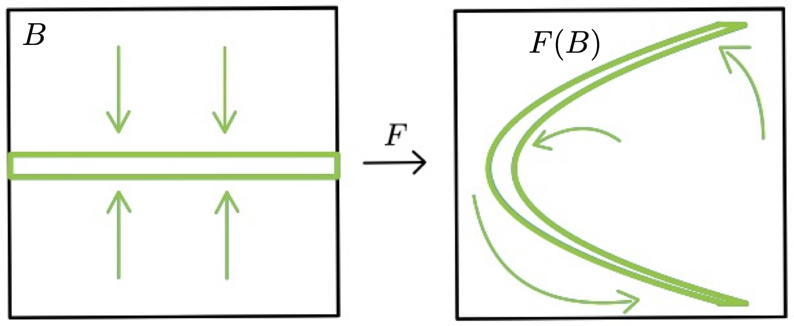
Figure 1. Hénon-like mapping.

We say that $F$ is Hénon-like renormalizable if there is a subdomain $\mathcal{B}^{1}\Subset B$ that is $R$-periodic:

$$F^{i}(\mathcal{B}^{1})\cap\mathcal{B}^{1}=\varnothing\text{, when $1\leq i<R$ \quad and \quad}F^{R}(\mathcal{B}^{1})\Subset\mathcal{B}^{1},$$

and the return map $F^{R}|_{\mathcal{B}^{1}}$ is again Hénon-like after a smooth change-of-coordinates $\Phi:\mathcal{B}^{1}\to B^{1}$, referred to as a straightening chart, that preserve the genuine horizontal foliation. In this case, the pair $(F^{R},\Phi)$ is referred to as a Hénon-like return. We define the (Hénon-like) renormalization $\mathcal{R}(F)$ of $F$ as the Hénon-like map obtained via a suitable affine rescaling of $\Phi\circ F^{R}\circ\Phi^{-1}$ that normalizes the width of the domain $B^{1}$. See Figure 2.

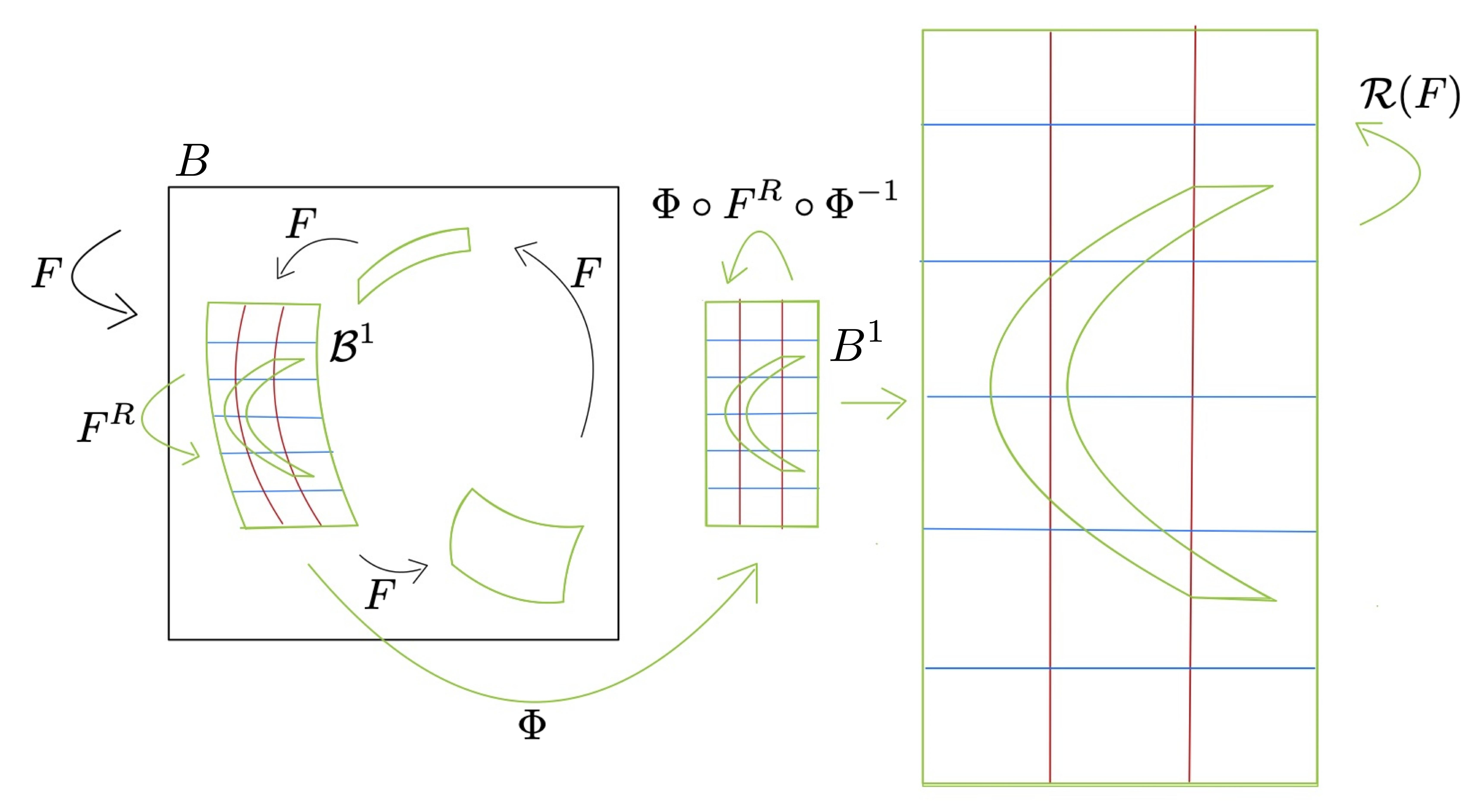
Figure 2. Hénon-like renormalization.

As in the one dimensional setting, one is confronted with the problem that the geometry of the new Hénon-like map may not be controlled. To address this issue, we incorporate Pesin theoretic ideas to the renormalization method. This involves keeping track of the regularity of points, which can then be used to control the geometry of dynamics in the higher-dimensional setting (see Appendix A). Loosely speaking, a Hénon-like return $(F^{R},\Phi:\mathcal{B}^{1}\to B^{1})$ is regular, and $F$ is regularly Hénon-like renormalizable if there is a sufficiently dominant exponential contraction of a vertical foliation of $\mathcal{B}^{1}$ under $F^{i}$ for $1\leq i\leq R$. For the precise definition, see Definition 2.1.

Remark 1.1.

As noted above, it is shown in [CLPY1] that for a regularly unicritical infinitely renormalizable diffeomorphism, the return maps are eventually regular Hénon-like.

The Hénon-like map $F:B\to B$ is $N$-times topologically renormalizable for some $N\in\mathbb{N}\cup\{\infty\}$ if there exist sequences

$$B=:\mathcal{B}^{0}\Supset\mathcal{B}^{1}\Supset\ldots\hskip 14.22636pt\text{and}\hskip 14.22636pt1=:R_{0}<R_{1}<\ldots$$

such that for $1\leq n\leq N$, the set $\mathcal{B}^{n}$ is an $R_{n}$-periodic Jordan domain. If there exists $\mathbf{b}\geq 2$ such that

$$r_{n-1}:=R_{n}/R_{n-1}\leq\mathbf{b}\hskip 14.22636pt\text{for all}\hskip 14.22636pt1\leq n\leq N,$$

then we say that the combinatorics of renormalization for $F$ is of ($\mathbf{b}$-)bounded type. Suppose for $1\leq n\leq N$, there exists a straightening chart $\Psi^{n}:\mathcal{B}^{n}\to B^{n}$ such that $(F^{R_{n}},\Psi^{n})$ is a Hénon-like return. Then the sequence

$$\{(F^{R_{n}},\Psi^{n}:\mathcal{B}^{n}\to B^{n})\}_{n=1}^{N}$$ (1.2)

is said to be nested. Conjugating $\Psi^{n}\circ F^{R_{n}}\circ(\Psi^{n})^{-1}$ by an affine map that normalizes the width of $B^{n}$, we obtain the $n$th renormalization $\mathcal{R}^{n}(F)$ of $F$.

In the one dimensional context, a priori bound refers to a uniform control of the distortion of the derivatives along renormalization intervals. For the two dimensional context, we propose to consider the distortion of the derivative along some particular type of curves. More precisely, consider a $C^{1}$-diffeomorphism $G:U\to G(U)$ defined on a domain $U\subset\mathbb{R}^{2}$. For a $C^{1}$-curve $\gamma\subset U$, let $\phi_{\gamma}:[0,|\gamma|]\to\gamma$ be the arc-length parameterization of $\gamma$. Denote $G_{\gamma}:=\phi_{G(\gamma)}\circ G\circ\phi_{\gamma}^{-1}$. The distortion of $G$ along $\gamma$ is defined as

$$\operatorname{Dis}(G,\gamma):=\sup_{s,t\in(0,|\gamma|)}\frac{|G_{\gamma}^{\prime}(s)|}{|G_{\gamma}^{\prime}(t)|}.$$

Main Theorem.

Consider a $C^{6}$-Hénon-like map $F:B\to B$. Suppose for $N\in\mathbb{N}\cup\{\infty\}$, the map $F$ has $N$ nested regular Hénon-like returns given by (1.2) with combinatorics of bounded type. For $1\leq n\leq N$, let $\gamma^{n}$ be a genuine horizontal arc contained in $\mathcal{B}^{n}$. Then $\operatorname{Dis}(F^{R_{n}},\gamma^{n})$ is uniformly bounded.

Remark 1.2.

In the Main theorem, the uniform bound on $\operatorname{Dis}(F^{R_{n}},\gamma^{n})$ depends only on certain finite geometric data about the map and the parameters of regularity (listed in (3.2) and (4.3)). In particular, the bound does not depend on $n$ or $N$.

Suppose that $N=\infty$. For $n\in\mathbb{N}$, consider the 1D profile $f_{n}:=\Pi_{\operatorname{1D}}\circ\mathcal{R}^{n}(F)$ of the $n$th renormalization of $F$. A consequence of the Main Theorem is that there exists a $C^{2}$-diffeomorphism $\phi_{n}$ and a constant $a_{n}\in\mathbb{R}$ such that the unimodal map $f_{n}$ decomposes into

$$f_{n}(\cdot)=(\phi_{n}(\cdot))^{2}+a_{n}.$$

It follows that the sequence $\{f_{n}\}_{n=1}^{\infty}$ is pre-compact in the space of unimodal maps in the $C^{1}$-topology.

1.2. Sketch of the Proof

The proof of a priori bounds for 1D unimodal maps relies on the Koebe Distortion Principle that controls the ratio distortion for compositions of 1D diffeomorphisms. This principle combines the Denjoy Lemma (that controls the distortion away from the critical points) with the negative Schwarzian derivative property near the critical points (that gives control of the cross ratio distortion at these moments). In turn, the Denjoy Lemma fundamentally relies on the disjointness of the intervals in the cycle of a periodic subinterval, which ensures that their total length remains uniformly bounded.

Turning to the 2D case, consider the regular Hénon-like returns given by (1.2). For concreteness, assume that $N=\infty$. For $n\geq 0$, we analyze how much distortion is induced on a horizontal cross-section $\mathcal{I}^{n}$ of the renormalization domain $\mathcal{B}^{n}$ by the return map $F^{R_{n}}$. However, in this 2D setting, it is not obvious whether the 1D Koebe Distortion Principle can still be applied. For instance, a union of disjoint arcs in 2D space may have arbitrarily large total length. Moreover, since a Hénon-like map is a diffeomorphism, it is not clear what, if anything, plays the role of its critical point. The following outlines our approach to overcoming these issues.

As our first task, we locate the dynamical critical value $v_{0}$ given by

$$\{v_{0}\}=\bigcup_{n=1}^{\infty}F^{R_{n}}(\mathcal{B}^{n}).$$

The point $v_{0}$ has a well-defined strong-stable manifold $W^{ss}(v_{0})$ and center manifold $W^{c}(v_{0})$ that have a quadratic tangency at $v_{0}$ (see Figure 3). Using the quantitative estimates provided in Appendix A, we prove that the vertical foliations on $\mathcal{B}^{n}$ induced by $\Psi^{n}$ converge super-exponentially fast to $W^{ss}(v_{0})$. Moreover, the image $F^{R_{n}}(\gamma_{h})$ of any horizontal arc $\gamma_{h}\subset\mathcal{B}^{n}$ is super-exponentially close to a subarc of $W^{c}(v_{0})$.

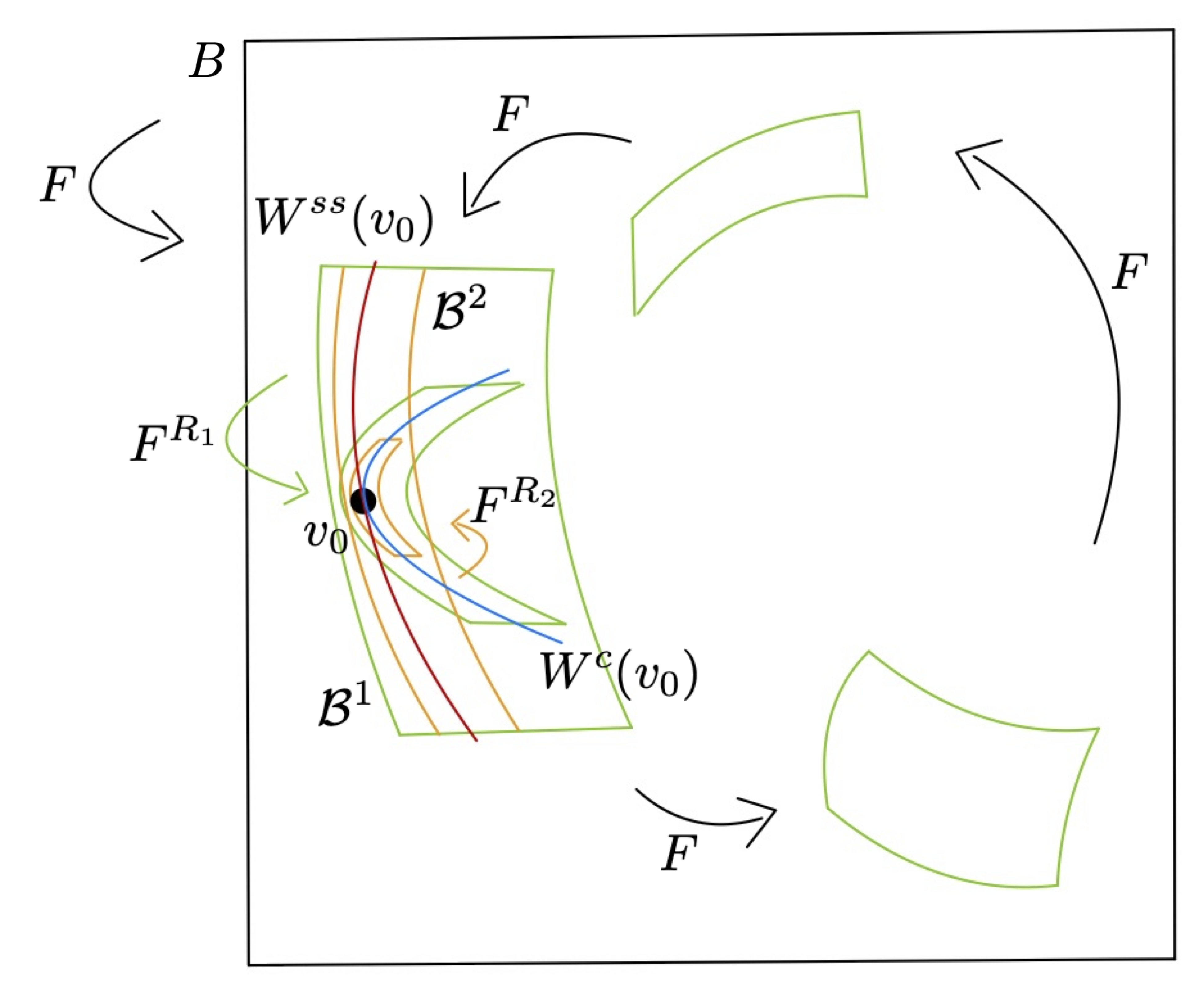
Figure 3. The critical value $v_{0}$ of an infinitely regularly Hénon-like renormalizable map $F$.

Assume that $\mathcal{I}^{m}\supset\mathcal{I}^{n}\ni v_{0}$ for $m\leq n$. For $n\geq n_{0}$ with $n_{0}\geq 0$ sufficiently large, there exists a well-defined projection map $\mathcal{P}^{n}:\mathcal{B}^{n}\to\mathcal{I}^{n}$ induced by the vertical foliation on $\mathcal{B}^{n}$. Since the vertical foliation on $\mathcal{B}^{n}$ converge super-exponentially to $W^{ss}(v_{0})$, and $W^{c}(v_{0})$ has a quadratic tangency with $W^{ss}(v_{0})$, applying $\mathcal{P}^{n}$ on a curve $\gamma$ sufficiently close to a subarc of $W^{c}(v_{0})$ has the effect of applying a 1D quadratic map near its critical point.

By replacing $F$ with $F^{n_{0}}$, we can assume that $n_{0}=0$. Then by applying the projections $\mathcal{P}^{m}$ for $0\leq m<n$, we can confine the orbit of $\mathcal{I}^{n}$ under $F$ to the fixed one-dimensional curve $\mathcal{I}^{0}$. This reduces the 2D dynamics of $F$ on $B=\mathcal{B}^{0}$ to the 1D mapping scheme on $\mathcal{I}^{0}$ that gives the transitions from one projected iterated image of $\mathcal{I}^{n}$ to another.

The main difficulty is that the foliation on $\mathcal{B}^{m}$, through which $\mathcal{P}^{m}$ is defined, is only invariant up to $R_{m}$ iterates. If $\mathcal{P}^{m}$ is naively applied to the part of the orbit of $\mathcal{I}^{n}$ contained in $\mathcal{B}^{m}$, then the resulting projections to $\mathcal{I}^{0}$ do not faithfully represent the original 2D dynamics of $F$ acting on $\mathcal{I}^{n}$. For example, if $m\ll n$, then it is possible that the projections under $\mathcal{P}^{m}$ of two iterated images of $\mathcal{I}^{n}$ are not disjoint.

For this reason, the 1D reduction must be done in a more careful way. At various moments in the orbit of $\mathcal{I}^{n}$, multiple projections from different scales of renormalization may be applied before they are “undone” to recover the original dynamics. In this procedure, we heavily rely on the fact that for bounded type combinatorics, the configuration of the cycle of $\mathcal{B}^{m+s}$ for $s\in\{1,2\}$ within $\mathcal{B}^{m}$ resembles the 1D combinatorial structure (including some 2D version of the Denjoy disjointedness property). Then once the 2D dynamics of $F$ is properly reduced to a 1D mapping scheme, the Koebe Distortion Principle can be applied to obtain the desired bound on the distortion.

1.3. Notations and conventions

Unless otherwise specified, we adopt the following notations and conventions.

Any diffeomorphism on a domain in $\mathbb{R}^{2}$ is assumed to be orientation-preserving. The projective tangent space at a point $p\in\mathbb{R}^{2}$ is denoted by $\mathbb{P}^{2}_{p}$.

Given a number $\eta>0$, we use $\bar{\eta}$ to denote any number that satisfy

$$\eta<\bar{\eta}<C\eta^{D}$$

for some uniform constants $C>1$ and $D>1$ (if $\eta>1$) or $D\in(0,1)$ (if $\eta<1$) that are independent of the map being considered. Additionally, we allow $\bar{\eta}$ to absorb any uniformly bounded coefficient or power. So for example, if $\bar{\eta}>1$, then we may write

$$\text{``}\;\;10\bar{\eta}^{5}=\bar{\eta}\;\;\text{''}.$$

Similarly, we use $\underline{\eta}$ to denote any number that satisfy

$$c\eta^{d}<\underline{\eta}<\eta$$

for some uniform constants $c\in(0,1)$ and $d\in(0,1)$ (if $\eta>1$) or $d>1$ (if $\eta<1$) that are independent of the map being considered. As before, we allow $\underline{\eta}$ to absorb any uniformly bounded coefficient or power. So for example, if $\underline{\eta}>1$, then we may write

$$\text{``}\;\;\tfrac{1}{3}\underline{\eta}^{1/4}=\underline{\eta}\;\;\text{''}.$$

These notations apply to any positive real number: e.g. ${\bar{\varepsilon}}>\varepsilon$, $\underline{\delta}<\delta$, ${\bar{L}}>L$, etc.

Note that $\bar{\eta}$ can be much larger than $\eta$ (similarly, $\underline{\eta}$ can be much smaller than $\eta$). Sometimes, we may avoid the $\bar{\eta}$ or $\underline{\eta}$ notation when indicating numbers that are somewhat or very close to the original value of $\eta$. For example, if $\eta\in(0,1)$ is a small number, then we may denote $\eta^{\prime}:=(1-\bar{\eta})\eta$. Then $\underline{\eta}\ll\eta^{\prime}<\eta$.

We use $n,m,i,j$ to denote integers (and less frequently $l,k$). The letter $i$ is never the imaginary number. Typically (but not always), $n\in\mathbb{N}$ and $m\in\mathbb{Z}$. We typically use $N,M$ to indicate fixed integers (often related to variables $n,m$).

We typically denote constants used for estimate bounds by $C,K\geq 1$ (less frequently $c>0$).

We use calligraphic font $\mathcal{U},\mathcal{T},\mathcal{I},$ etc, for objects in the phase space and regular fonts $U,T,I,$ etc, for corresponding objects in the linearized/uniformized coordinates. A notable exception are for the invariant manifolds $W^{ss},W^{c}$.

We use $p,q$ to indicate points in the phase space, and $z,w$ for points in linearized/uniformized coordinates.

For any set $X_{m}\subset\Omega$ with a numerical index $m\in\mathbb{Z}$, we denote

$$X_{m+l}:=F^{l}(X_{m})$$

for all $l\in\mathbb{Z}$ for which the right-hand side is well-defined. Similarly, for any direction $E_{p_{m}}\in\mathbb{P}^{2}_{p_{m}}$ at a point $p_{m}\in\Omega$, we denote

$$E_{p_{m+l}}:=DF^{l}(E_{p_{m}}).$$

Define

$$\pi_{h}(x,y):=x,\hskip 14.22636pt\pi_{v}(x,y):=y,\hskip 14.22636pt\Pi_{h}(x,y):=(x,0)\hskip 14.22636pt\text{and}\hskip 14.22636pt\Pi_{v}(x,y):=(0,y).$$

2. Precise Definitions

2.1. Charts

For $z\in\mathbb{R}^{2}$, denote the space of tangent directions at $z$ by $\mathbb{P}^{2}_{z}$. Let $E^{gv}_{z},E^{gh}_{z}\in\mathbb{P}^{2}_{z}$ be the genuine vertical and horizontal directions at $z$ respectively.

A $C^{r}$-chart is a $C^{r}$-diffeomorphism $\Phi:\mathcal{B}\to B$ from a quadrilateral $\mathcal{B}\subset\mathbb{R}^{2}$ to a rectangle $B=I\times J\subset\mathbb{R}^{2}$, where $I,J\subset\mathbb{R}$ are intervals. The vertical/horizontal direction $E^{v/h}_{p}\in\mathbb{P}^{2}_{p}$ at $p\in\mathcal{B}$ (associated to $\Phi$) are given by

$$E^{v/h}_{p}:=D\Phi^{-1}\left(E^{gv/gh}_{\Phi(p)}\right).$$

The chart $\Phi$ is said to be genuinely vertical/horizontal if $E^{v/h}_{p}=E^{gv/gh}_{p}$ for all $p\in\mathcal{B}$.

A vertical leaf in $\mathcal{B}$ is a curve $l^{v}$ such that

$$l^{v}\subseteq\Phi^{-1}(\{a\}\times\pi_{v}(B))\hskip 14.22636pt\text{for some}\hskip 14.22636pta\in\pi_{h}(B).$$

If the above containment is an equality, then $l^{v}$ is said to be full. A (full) horizontal leaf $l^{h}$ in $\mathcal{B}$ is defined analogously.

Let $p\in\mathcal{B}$ and $E_{p}\in\mathbb{P}^{2}_{p}$. Denote $z:=\Phi(p)$ and $E_{z}:=D\Phi(E_{p}).$ For $t>0$, the direction $E_{p}$ is said to be $t$-vertical in $\mathcal{B}$ if

$$\frac{\measuredangle(E_{z},E_{z}^{gv})}{\measuredangle(E_{z},E_{z}^{gh})}<t.$$

A $t$-horizontal direction in $\mathcal{B}$ is analogously defined.

A $C^{0}$-curve $\Gamma^{v}\subset\mathcal{B}$ is said to be vertical in $\mathcal{B}$ if $\Phi(\Gamma^{v})$ is a vertical graph in $B$ in the usual sense. That is, there exists an interval $I^{v}\subseteq\pi_{v}(B)$ and a map $g_{v}:I^{v}\to\pi_{h}(B)$ such that

$$\Phi(\Gamma^{v})=\mathcal{G}^{v}(g_{v}):=\{(g_{v}(y),y)\;|\;y\in I^{v}\}.$$

If $I^{v}=\pi_{v}(B)$, then $\Gamma^{v}$ is said to be vertically proper in $\mathcal{B}$. A horizontal or a horizontally proper curve $\Gamma^{h}$ in $\mathcal{B}$ is analogously defined. If $\Gamma^{v}$ is $C^{r}$, and $\|g_{v}^{\prime}\|_{C^{r-1}}\leq t$ for some $t\geq 0$, then we say that $\Gamma^{v}$ is $t$-vertical (in $C^{r}$) in $\mathcal{B}$. Note that $\Gamma^{v}$ is a (vertically proper) $0$-vertical curve if and only if it is a (full) vertical leaf.

If $\Gamma^{v}$ is $C^{2}$, and $g_{v}$ has a unique critical point $c\in I^{v}$ of quadratic type: $g_{v}^{\prime}(c)=0$ and

$$\kappa_{\Phi}(\Gamma^{v}):=g_{v}^{\prime\prime}(c)\neq 0,$$ (2.1)

then $\Gamma^{v}$ is a vertical quadratic curve in $\mathcal{B}$. We refer to $\kappa_{\Phi}(\Gamma^{v})$ as the valuable curvature of $\Gamma^{v}$ in $\mathcal{B}$.

Let $\mathcal{E}^{v}:\mathcal{B}\to T^{1}(\mathcal{B})$ be the $C^{r-1}$-unit vector field given by

$$\mathcal{E}^{v}(p):=D\Phi^{-1}(E^{gv}_{\Phi(p)}).$$

A $C^{r-1}$-unit vector field ${\tilde{\mathcal{E}}}^{v}:\mathcal{U}\to T^{1}(\mathcal{U})$ defined on a domain $\mathcal{U}\subset\mathcal{B}$ is said to be $t$-vertical in $C^{r-1}$ in $\mathcal{B}$ for some $t\geq 0$ if $\|{\tilde{\mathcal{E}}}^{v}-\mathcal{E}^{v}\|_{C^{r-1}}\leq t$.

Let $\tilde{\Phi}:\tilde{\mathcal{B}}\to\tilde{B}$ be another chart with $\tilde{\mathcal{B}}\subset\mathcal{B}$. We define the following relations between $\Phi$ and $\tilde{\Phi}$.

• We say that $\tilde{\mathcal{B}}$ is vertically proper in $\mathcal{B}$ if every full vertical leaf in $\tilde{\mathcal{B}}$ is vertically proper in $\mathcal{B}$.

• We say that $\Phi$ and $\tilde{\Phi}$ are horizontally equivalent on $\tilde{\mathcal{B}}$ if every horizontal leaf in $\tilde{\mathcal{B}}$ is a horizontal leaf in $\mathcal{B}$.

• For $t\geq 0$, we say that $\tilde{\mathcal{B}}$ is $t$-vertical in $\mathcal{B}$ if $\Phi$ and $\tilde{\Phi}$ are horizontally equivalent, and the unit vector field given by

  $${\tilde{\mathcal{E}}}^{v}(p):=D\tilde{\Phi}^{-1}(E^{gv}_{\tilde{\Phi}(p)})\hskip 14.22636pt\text{for}\hskip 14.22636ptp\in\tilde{\mathcal{B}}$$

  is $t$-vertical in $C^{r-1}$ in $\mathcal{B}$.

• We say that $\Phi$ and $\tilde{\Phi}$ are equivalent on $\tilde{\mathcal{B}}$ if $\tilde{\mathcal{B}}$ is $0$-vertical in $\mathcal{B}$.

Let $\Psi:\mathcal{B}\to B$ be a chart satisfying the following properties.

• There exists $q\in\mathcal{B}$ such that $\Psi(q)=0\in B$.

• Let

  $$\mathcal{I}^{h}(t):=\Psi^{-1}(t,0)\hskip 14.22636pt\text{for}\hskip 14.22636ptt\in\pi_{h}(B),$$

  and

  $$\mathcal{I}^{v}(s):=\Psi^{-1}(0,s)\hskip 14.22636pt\text{for}\hskip 14.22636pts\in\pi_{v}(B).$$

  Then $\|(\mathcal{I}^{h/v})^{\prime}\|\equiv 1$.

In this case, we say that $\Psi$ is centered (at $q$). Clearly, for any chart $\Phi:\mathcal{B}\to D$ and any point $q\in\mathcal{B}$, there exists a unique chart $\Psi:\mathcal{B}\to B$ equivalent to $\Phi$ that is centered at $q$.

Suppose that $\Psi:(\mathcal{B},q)\to(B,0)$ is centered at some point $q\in\mathcal{B}$. Let $\Gamma^{h}\subset\mathcal{B}$ be a horizontal $C^{r}$-curve, so that $\Psi(\Gamma^{h})$ is the horizontal graph in $B$ of a $C^{r}$-map $g_{h}:I^{h}\to\pi_{v}(B)$ defined on an interval $I^{h}\subset\pi_{h}(B)$. We say that $\Gamma^{h}$ is $t$-horizontal in $C^{r}$ in $\mathcal{B}$ if $\|g_{h}\|_{C^{r}}\leq t$. In particular, $\Gamma^{h}$ is $0$-horizontal in $\mathcal{B}$ if and only if $\Gamma^{h}$ is a subarc of the full horizontal leaf containing $q$.

2.2. Regularity

For an integer $r\geq 2$, consider a $C^{r}$-diffeomorphism $F:B\to F(B)\Subset B$ defined on a domain $B\subset\mathbb{R}^{2}$. Let $L\geq 1$; $\varepsilon,\lambda\in(0,1)$ and $M\in\mathbb{N}\cup\{\infty\}$. A point $p\in B$ is $M$-times forward $(L,\varepsilon,\lambda)$-regular along $E_{p}^{+}\in\mathbb{P}^{2}_{p}$ if for $s\in\{0,1\}$, we have

$$L^{-1}\lambda^{(1+\varepsilon)m}\leq\frac{\|DF^{m}|_{E^{+}_{p}}\|^{s+1}}{(\operatorname{Jac}_{p}F^{m})^{s}}\leq L\lambda^{(1-\varepsilon)m}\hskip 14.22636pt\text{for all}\hskip 14.22636pt1\leq m\leq M.$$ (2.2)

Intuitively, when $s=0$, the condition gives exponential contraction along $E_{p}$, and when $s=1$, it gives the domination of this contraction (there is exponential repulsion in the projective tangent space of other directions from $E_{p}$). Similarly, $p$ is $M$-times backward $(L,\varepsilon,\lambda)$-regular along $E^{-}_{p}\in\mathbb{P}^{2}_{p}$ if for $s\in\{0,1\}$,

$$L^{-1}\lambda^{(1+\varepsilon)m}\leq\frac{(\operatorname{Jac}_{p}F^{-m})^{s}}{\|DF^{-m}|_{E^{-}_{p}}\|^{s+1}}\leq L\lambda^{(1-\varepsilon)m}\hskip 14.22636pt\text{for all}\hskip 14.22636pt1\leq m\leq M.$$ (2.3)

The constants $L$, $\varepsilon$ and $\lambda$ are referred to as an irregularity factor, a marginal exponent and a contraction base respectively.

If $\varepsilon$ is sufficiently small (independently of $F$), then the local dynamics of $F$ near the forward (or backward resp.) orbit of $p$ can be quasi-linearized up to the $M$th iterate, see Theorem A.2. If $M=\infty$, this implies in particular that $p$ has a $C^{r}$-smooth strong-stable manifold (or center manifold resp.), see Theorem A.15. It should be noted that the center manifold at an infinitely backward regular point $p$ is not uniquely defined; however, its $C^{r}$-jet at $p$ is unique, see Theorem A.16. Henceforth, any marginal exponent will be assumed to be sufficiently small.

Definition 2.1.

Let $F:B\to B$ be a Hénon-like map. A Hénon-like return $(F^{R},\Phi:\mathcal{B}^{1}\to B^{1})$ is said to be $(L,\varepsilon,\lambda)$-regular if the following conditions hold. Let

$$E_{p}^{v/h}:=D\Psi^{-1}\left(E^{gv/gh}_{\Psi(p)}\right).$$

• Every $p\in\mathcal{B}^{1}$ is $R$-times forward $(L,\varepsilon,\lambda)$-regular along $E^{v}_{p}$.

• Every $q\in F^{R}(\mathcal{B}^{1})\Subset\mathcal{B}^{1}$ is $R$-times backward $(L,\varepsilon,\lambda)$-regular along $E^{h}_{q}$.

• For any $p\in\mathcal{B}^{1}$, we have $\measuredangle(E^{v}_{p},E^{h}_{p})>1/L$.

In this case, we say that $F$ is $(L,\varepsilon,\lambda)$-regularly Hénon-like renormalizable.

3. Convergence of the Straightening Charts

Let $r\geq 2$ be an integer, and consider a $C^{r+1}$-Hénon-like map $F:B\to B$. For some $N\in\mathbb{N}\cup\{\infty\}$; $L\geq 1$ and $\varepsilon,\lambda\in(0,1)$, suppose that $F$ has $N$ nested $(L,\varepsilon,\lambda)$-regular Hénon-like returns given by (1.2). Furthermore, assume that $N$ is sufficiently large, so that for some smallest number $0\leq n_{0}\leq N$, we have

$$\overline{K_{0}}\lambda^{\varepsilon R_{n_{0}}}<\eta,$$ (3.1)

where $\eta\in(0,1)$ is independent of $F$, and

$${K_{0}}={K_{0}}(L,\lambda,\varepsilon,\lambda^{1-\varepsilon}\|DF^{-1}\|,\|DF\|_{C^{r}},r)\geq 1$$ (3.2)

is a uniform constant.

For $n_{0}\leq n\leq N$ and $m\in\mathbb{Z}$, denote $\mathcal{B}^{n}_{m}:=F^{m}(\mathcal{B}^{n})$. Observe that $\mathcal{B}^{n+1}_{R_{n+1}}\Subset\mathcal{B}^{n}_{R_{n}}.$ Let

$$v_{0}\in\mathcal{Z}_{0}:=\bigcap_{n=1}^{N}\mathcal{B}^{n}_{R_{n}},$$

be a point to be specified later (as the critical value of $F$). Without loss of generality, assume that $\Psi^{n}$ is centered at $v_{0}$.

In this section, we describe the asymptotic behavior of the centered straightening charts $\{\Psi^{n}\}_{n=1}^{N}$ for the renormalizations of $F$.

Remark 3.1.

In this section, we do not assume that the combinatorics of the renormalizations of $F$ is necessarily of bounded type.

Define

$$I^{n}_{0}:=\pi_{h}(B^{n}_{0})\hskip 14.22636pt\text{and}\hskip 14.22636pt\mathcal{I}^{n}_{0}:=(\Psi^{n})^{-1}(I^{n}_{0}\times\{0\}).$$

Then it follows that $I^{n}_{0}\Subset I^{1}_{0}$ and $\Psi^{n}|_{\mathcal{I}^{n}_{0}}=\Psi^{1}|_{\mathcal{I}^{n}_{0}}.$ Denote $\mathcal{I}^{n}_{m}:=F^{m}(\mathcal{I}^{n}_{0})$ for $m\in\mathbb{Z}$.

For $p_{0}\in\mathcal{B}^{n}_{0}$, write $z_{0}:=\Psi^{n}(p_{0})$, and let

$$E^{h}_{p_{0}}:=D(\Psi^{n})^{-1}(E^{gh}_{z_{0}})\hskip 14.22636pt\text{and}\hskip 14.22636ptE^{v,n}_{p_{0}}:=D(\Psi^{n})^{-1}(E^{gv}_{z_{0}}).$$

Additionally, let

$$E^{h,n}_{p_{R_{n}-1}}:=DF^{R_{n}-1}(E^{h}_{p_{0}})\hskip 14.22636pt\text{and}\hskip 14.22636ptE^{v}_{p_{R_{n}-1}}:=DF^{-1}(E^{h}_{p_{R_{n}}})=DF^{R_{n}-1}(E^{v,n}_{p_{0}}).$$

By increasing $L$ by a uniform amount if necessary (see Proposition A.1), we may assume that every $q\in\mathcal{B}^{n}_{R_{n}-1}$ is $(R_{n}-1)$-times backward $(L,\varepsilon,\lambda)$-regular along $E^{v}_{q}$.

Proposition 3.2 (Vertical extension of charts).

For $n_{0}\leq n\leq N$, the $n$th centered straightening chart can be extended to $\Psi^{n}:\hat{\mathcal{B}}^{n}_{0}\to\hat{B}^{n}_{0}$ such that the following properties hold.

1. The quadrilateral $\hat{\mathcal{B}}^{n}_{0}$ is vertically proper and $\eta$-vertical in $\mathcal{B}^{n_{0}}_{0}$.

2. We have $\|(\Psi^{n})^{\pm 1}\|_{C^{r}}<{K_{0}}$, and

   $$\|\Psi^{n}\circ(\Psi^{n+1})^{-1}-\operatorname{Id}\|_{C^{r}}<\lambda^{(1-{\bar{\varepsilon}})R_{n}}.$$ (3.3)

3. Every point $q_{0}\in\hat{\mathcal{B}}^{n}_{0}$ is $R_{n}$-times forward $({K_{0}},\varepsilon,\lambda)$-regular along $E^{v,n}_{q_{0}}$.

Proof.

For $p_{0}\in\mathcal{B}^{n}_{0}$, let

$$\{\Phi_{p_{m}}:\mathcal{U}_{p_{m}}\to U_{p_{m}}\}_{m=0}^{R_{n}}$$

be a linearization of $F$ along the $R_{n}$ forward orbit of $p_{0}$ with vertical direction $E^{v,n}_{p_{0}}$. Let $\mathcal{E}^{v,n}_{p_{m}}:\mathcal{U}_{p_{m}}\to T^{1}(\mathcal{U}_{p_{m}})$ be the $C^{r}$-unit vector field given by $\mathcal{E}^{v,n}_{p_{m}}(q)\in E^{v,n}_{q}$ for $q\in\mathcal{U}_{p_{m}}.$

Let $l^{v,{n_{0}}}_{p_{0}}$ be the full vertical leaf in $\mathcal{B}^{n_{0}}_{0}$ containing $p_{0}$. For $q_{0}\in l^{v,n_{0}}_{p_{0}}$, let

$$\{\Phi_{q_{m}}:\mathcal{U}_{q_{m}}\to U_{q_{m}}\}_{m=0}^{R_{n_{0}}}$$

be a linearization of $F$ along the $R_{n_{0}}$ forward orbit of $q_{0}$ with vertical direction $E^{v,{n_{0}}}_{q_{0}}$ given by Theorem A.2.

Let $M$ be a nearest integer to $R_{n_{0}}/2$. By Lemma A.3, we see that $\mathcal{U}_{p_{M}}\supset\mathbb{D}_{p_{M}}\left(\lambda^{{\bar{\varepsilon}}M}\right).$ Lemma A.11 implies that Corollary A.8 applies to all points in the $M$-times truncated regular neighborhood $\mathcal{U}_{q_{0}}^{M}$ at $q_{0}$. The $R_{n_{0}}$-times forward regularity at all points in $\mathcal{B}^{n_{0}}_{0}$ together with (3.1) implies that

$$\check{\mathcal{U}}_{q_{M}}:=F^{M}(\mathcal{U}_{q_{0}}^{M})\subset\mathcal{U}_{p_{M}}.$$

By Proposition A.1, $q_{M}$ and $p_{M}$ are $M$-times forward $(\lambda^{-{\bar{\varepsilon}}M},\varepsilon,\lambda)_{v}$-regular along $E^{v,{n_{0}}}_{q_{M}}$ and $E^{v,n}_{p_{M}}$ respectively. Hence, Proposition A.9 implies that $\mathcal{E}^{v,n}_{p_{M}}|_{\check{\mathcal{U}}_{q_{M}}}$ is $\lambda^{(1-{\bar{\varepsilon}})M}$-vertical in $C^{0}$ in $\mathcal{U}_{q_{M}}$. Moreover, the bounds on $\|\Phi_{p_{M}}\|_{C^{r}}$ and $\|\Phi_{q_{M}}\|_{C^{r}}$ given by Theorem A.2 imply that

$$\|D\Phi_{q_{M}}(\mathcal{E}^{v,n}_{p_{M}})\|_{C^{r-1}}<\lambda^{-{\bar{\varepsilon}}M}.$$

Extend $\mathcal{E}^{v,n}_{p_{0}}$ to $\mathcal{U}_{q_{0}}^{M}$ as

$$\mathcal{E}^{v,n}_{p_{0}}|_{\mathcal{U}_{q_{0}}^{M}}:=DF^{-M}(\mathcal{E}^{v,n}_{p_{M}}|_{\check{\mathcal{U}}_{q_{M}}}).$$

Then by Proposition A.14, we have

$$\|\mathcal{E}^{v,n}_{p_{0}}-\mathcal{E}^{v,{n_{0}}}_{q_{0}}\|_{C^{r}}\leq\lambda^{(1-{\bar{\varepsilon}})M}(1+\|D\Phi_{q_{0}}^{-1}\|_{C^{r-1}})(1+\|D\Phi_{q_{M}}(\mathcal{E}^{v,n}_{p_{M}})\|_{C^{r-1}})\leq\eta.$$

Rectifying the vertical directions near $l^{v,{n_{0}}}_{p_{0}}$ given by $\mathcal{E}^{v,n}_{p_{0}}$, we obtain the desired extension of $\Psi^{n}$.

Observe that for $0\leq k\leq M$

$$\measuredangle(E^{v,n}_{q_{k}},E^{v,n_{0}}_{q_{k}})<\lambda^{(1-{\bar{\varepsilon}})(R_{n_{0}}-k)}.$$

It follows that

$$\frac{1}{\sqrt{2}}<\frac{\|DF^{k}|_{E^{v,n}_{q_{0}}}\|}{\|DF^{k}|_{E^{v,{n_{0}}}_{q_{0}}}\|}<\sqrt{2}.$$

Concatenating with the forward $M$-times $(\lambda^{-{\bar{\varepsilon}}M},\varepsilon,\lambda)$-regularity of $q_{M}$, we see that

$$\frac{\lambda^{{\bar{\varepsilon}}M}}{\sqrt{2}L}\lambda^{(1+\varepsilon)(M+i)}\leq\|DF^{M+i}|_{E^{v,n}_{q_{0}}}\|\leq\sqrt{2}L\lambda^{-{\bar{\varepsilon}}M}\lambda^{(1-\varepsilon)(M+i)}.$$

Since $n_{0}$ is assumed to be the smallest number that satisfies (3.1), we have $\lambda^{-{\bar{\varepsilon}}M}<K_{0}$. The claimed $R_{n}$-times forward regularity of $q_{0}$ along $E^{v,n}_{q_{k}}$ follows.

Lastly, replacing the renormalization depth ${n_{0}}$ in the above argument by $n$, we obtain (3.3). ∎

Consider $C^{r}$-curves $\Gamma_{1},\Gamma_{2}\subset\mathbb{R}^{2}$ with $|\Gamma_{1}|\geq|\Gamma_{2}|$. For $i\in\{1,2\}$, let $\phi_{\Gamma_{i}}:J_{i}\subset\mathbb{R}\to\Gamma_{i}$ be a parameterization of $\Gamma_{i}$ such that

• $|\phi_{\Gamma_{i}}^{\prime}|\equiv 1$;

• $J_{1}\supset J_{2}$;

• $\|\phi_{\Gamma_{1}}|_{J_{2}}-\phi_{\Gamma_{2}}\|_{C^{r}}$ is minimal.

In this case, define

$$\|\Gamma_{1}\|_{C^{r}}:=\|\phi_{\Gamma_{1}}\|\hskip 14.22636pt\text{and}\hskip 14.22636pt\operatorname{dist}_{C^{r}}(\Gamma_{1},\Gamma_{2}):=\|\phi_{\Gamma_{1}}|_{J_{2}}-\phi_{\Gamma_{2}}\|_{C^{r}}.$$ (3.4)

Lemma 3.3.

For $n_{0}\leq n\leq N$, let $l^{n}_{0}$ be a full horizontal leaf in $\hat{\mathcal{B}}^{n}_{0}$. Denote $l^{n}_{m}:=F^{m}(l^{n}_{0})$ for $m\in\mathbb{Z}$. Then we have $\|l^{n}_{R_{n}-1}\|_{C^{r}}<{K_{0}}$; and

$$\operatorname{dist}_{C^{r}}(l^{n}_{R_{n}-1},l^{n+1}_{R_{n+1}-1})<\lambda^{(1-{\bar{\varepsilon}})R_{n}}.$$

Proof.

For $p_{-1}\in\mathcal{Z}_{-1}:=F^{-1}(\mathcal{Z}_{0}),$ let

$$\{\Phi_{p_{-m}}:\mathcal{U}_{p_{-m}}\to U_{p_{-m}}\}_{m=1}^{R_{N}}$$

be a linearization of $F$ along the $R_{N}$-times backward orbit of $p_{-1}$ with vertical direction $E^{v}_{p_{-1}}$ (if $N=\infty$, then $R_{\infty}=\infty$). Let $\mathcal{V}_{-R_{n}}$ be the connected component of $F^{-R_{n}+1}(\mathcal{U}_{p_{-1}}^{R_{n}})\cap\hat{\mathcal{B}}^{n}_{0}$ containing $p_{-R_{n}}$. Note that $\Psi^{n}|_{\mathcal{V}_{-R_{n}}}$ defines a chart on $\mathcal{V}_{-R_{n}}$, so that $\mathcal{V}_{-R_{n}}$ is $0$-vertical in $\hat{\mathcal{B}}^{n}_{0}$. Moreover, arguing as in the proof of Proposition 3.2, we see that $\mathcal{V}_{-R_{n}}$ is also vertically proper in $\hat{\mathcal{B}}^{n}_{0}$.

Consider the map

$$H_{n}(x,y)=(h_{n}(x),e_{n}(x,y)):=\Phi_{p_{-1}}\circ F^{R_{n}-1}\circ(\Psi^{n})^{-1}(x,y)$$

for $(x,y)\in\Psi^{n}(\mathcal{V}_{-R_{n}})$. Denote

$$F_{p_{-n}}:=\Phi_{p_{-n+1}}\circ F\circ(\Phi_{p_{-n}})^{-1}.$$

Then

$$H_{n}=F_{p_{-2}}\circ\ldots\circ F_{p_{-R_{n}}}\circ\Phi_{p_{-R_{n}}}\circ(\Psi^{n})^{-1}.$$ (3.5)

By Theorem A.2, we see that

$$\|\Phi_{p_{-R_{n}}}\circ(\Psi^{n})^{-1}\|_{C^{r}}<\lambda^{-{\bar{\varepsilon}}R_{n}}.$$

Applying Proposition A.12, we conclude that

$$\|e_{n}\|_{C^{r}}<\lambda^{(1-{\bar{\varepsilon}})R_{n}}.$$ (3.6)

The result follows. ∎

Proposition 3.4 (Locating the critical value).

If $N=\infty$, then the following statements hold.

1. For any point $p_{0}\in\mathcal{Z}_{0}$, there exists a unique strong stable direction $E^{ss}_{p_{0}}\in\mathbb{P}^{2}_{p_{0}}$ such that

   $$\|E^{v,n}_{p_{0}}-E^{ss}_{p_{0}}\|<\lambda^{(1-{\bar{\varepsilon}})R_{n}}\hskip 14.22636pt\text{for}\hskip 14.22636ptn\geq n_{0}.$$

   Moreover, $p_{0}$ is infinitely forward $(L,\varepsilon,\lambda)$-regular along $E^{ss}_{p_{0}}$.

2. Any point $p_{-1}\in\mathcal{Z}_{-1}:=F^{-1}(\mathcal{Z}_{0})$ is infinitely backward $(L,\varepsilon,\lambda)$-regular along $E^{v}_{p_{-1}}$. Moreover, there exists a unique center direction $E^{c}_{p_{-1}}\in\mathbb{P}^{2}_{p_{-1}}$ such that

   $$\|E^{h,n}_{p_{-1}}-E^{c}_{p_{-1}}\|<\lambda^{(1-{\bar{\varepsilon}})R_{n}}\hskip 14.22636pt\text{for}\hskip 14.22636ptn\geq n_{0}.$$

3. There exists a unique point $v_{0}\in\mathcal{Z}_{0}$ such that

   $$E^{ss}_{v_{0}}=DF(E^{c}_{v_{-1}}).$$

   Moreover, the strong stable manifold $W^{ss}(v_{0})$ and the center manifold $F(W^{c}(v_{-1}))$ have a quadratic tangency at $v_{0}$.

Proof.

The first and second claim follow immediately from Propositions A.9 and A.10.

For $n\geq n_{0}$, recall that $\mathcal{I}^{n}_{R_{n}}$ is a vertical quadratic curve in $\mathcal{B}^{n}_{0}$. Let $v^{n}_{0}\in\mathcal{I}^{n}_{0}$ be the unique point such that

$$E^{v,n}_{v^{n}_{R_{n}}}=DF^{R_{n}}(E^{h}_{v^{n}_{0}}).$$

By Proposition 3.2 and Lemma 3.3, we have

$$\operatorname{dist}(v^{n}_{R_{n}},v^{n+1}_{R_{n+1}})<\lambda^{(1-{\bar{\varepsilon}})R_{n}}.$$

Thus, there exists a unique point $v_{0}\in\mathcal{Z}_{0}$ such that

$$\operatorname{dist}(v^{n}_{R_{n}},v_{0})<\lambda^{(1-{\bar{\varepsilon}})R_{n}}\hskip 14.22636pt\text{and}\hskip 14.22636pt\operatorname{dist}_{C^{r}}(\mathcal{I}^{n}_{R_{n}},W^{c}(v_{0}))<\lambda^{(1-{\bar{\varepsilon}})R_{n}}.$$

By (3.3), we see that $W^{ss}(v_{0})$ and $W^{c}(v_{0})$ have a quadratic tangency at $v_{0}$.

Lastly, let $\mathcal{U}_{v_{0}}$ be a neighborhood of $v_{0}$. Then there exists a uniform constant $k>0$ such that for all $n$ sufficiently large, if $p_{R_{n}}\in\mathcal{I}^{n}_{R_{n}}\setminus\mathcal{U}_{v_{0}}$ then

$$\measuredangle(E^{v,n}_{p_{R_{n}}},DF^{R_{n}}(E^{h}_{p_{0}}))>k.$$

Thus, $v_{0}$ is the unique point in $\mathcal{Z}_{0}$ satisfying $E^{ss}_{v_{0}}=E^{c}_{v_{0}}.$ ∎

We define the critical value $v_{0}\in\mathcal{Z}_{0}$ as follows. If $N=\infty$, let $v_{0}$ be the point given in Proposition 3.4 iii). Otherwise, let $v_{0}$ be the unique point in $\mathcal{I}^{N}_{R_{N}}$ such that

$$DF^{R_{N}}(E^{h}_{v_{-R_{N}}})=E^{v,N}_{v_{0}}$$

(recall that such a point exists since $\mathcal{I}^{N}_{R_{N}}$ is a vertical quadratic curve in $\mathcal{B}^{N}_{0}$). Define the critical point as $v_{-1}:=F^{-1}(v_{0})$.

Theorem 3.5 (Valuable charts).

Let ${K_{0}}\geq 1$ be the constant given in (3.2). There exist charts

$$\Phi_{0}:(\mathcal{B}_{0},v_{0})\to(B_{0},0)\hskip 14.22636pt\text{and}\hskip 14.22636pt\Phi_{-1}:(\mathcal{B}_{-1},v_{-1})\to(B_{-1},0)$$

such that

• $\Phi_{0}$ is centered at $v_{0}$ and is genuine horizontal;

• $\mathcal{B}_{0}\supset\mathcal{B}^{n_{0}}_{0}$, $\mathcal{B}_{-1}\supset\mathcal{B}^{n_{0}}_{R_{n_{0}}-1}$ and $F(\mathcal{B}_{-1})\Subset\mathcal{B}_{0}$;

• $\|\Phi_{i}^{\pm 1}\|_{C^{r}}<{K_{0}}$ for $i\in\{0,-1\}$; and

• we have

  $$\Phi_{0}\circ F\circ\Phi_{-1}^{-1}(x,y)=(f_{0}(x)-\lambda y,x)\hskip 14.22636pt\text{for}\hskip 14.22636pt(x,y)\in B_{-1},$$ (3.7)

  where $f_{0}:(\pi_{h}(B_{-1}),0)\to(\pi_{h}(B_{0}),0)$ is a $C^{r}$-map that has a unique critical point at $0$ such that

  $$\|f_{0}^{\prime\prime}\|_{C^{r-2}}<{K_{0}}\hskip 14.22636pt\text{and}\hskip 14.22636pt\kappa_{F}:=\inf_{x\in\pi_{h}(B_{-1})}f_{0}^{\prime\prime}(x)>0.$$ (3.8)

Moreover, the following properties hold for $n_{0}\leq n\leq N$.

1. We have

   $$\|\Phi_{0}\circ(\Psi^{n})^{-1}-\operatorname{Id}\|_{C^{r}}<\lambda^{(1-{\bar{\varepsilon}})R_{n}}.$$

2. Let

   $$H_{n}:=\Phi_{-1}\circ F^{R_{n}-1}\circ(\Psi^{n})^{-1}.$$

   Then $H_{n}(x,y)=(h_{n}(x),e_{n}(x,y))$, where $h_{n}:I^{n}_{0}\to h_{n}(I^{n}_{0})$ is a $C^{r}$-diffeomorphism and $e_{n}$ is a $C^{r}$-map such that

   $$\lambda^{{\bar{\varepsilon}}R_{n}}<|h_{n}^{\prime}(x)|<\lambda^{-{\bar{\varepsilon}}R_{n}}\hskip 14.22636pt\text{for}\hskip 14.22636ptx\in I^{n}_{0}\hskip 14.22636pt\text{and}\hskip 14.22636pt\|e_{n}\|_{C^{r}}<\lambda^{(1-{\bar{\varepsilon}})R_{n}}.$$ (3.9)

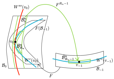
Figure 4. Geometry near the critical value $v_{0}$ and the critical point $v_{-1}$ (if $N=\infty$). For $n\geq n_{0}$, we have $v_{0}\in\hat{\mathcal{B}}^{n}_{0}\subset\mathcal{B}_{0}$ and $v_{-1}\in\hat{\mathcal{B}}^{n}_{R_{n}-1}\subset\mathcal{B}_{-1}$. There exist charts $\Phi_{0}:\mathcal{B}_{0}\to B_{0}$ and $\Phi_{-1}:\mathcal{B}_{-1}\to B_{-1}$ such that $\Phi_{0}\circ F\circ\Phi_{-1}$ is Hénon-like (see (3.7)). The charts $\Psi^{n}$ converges to $\Phi_{0}$

Proof.

For $t\geq 0$ and $X\subset\mathbb{R}^{2}$, denote

$$X(t):=\{p\in\mathbb{R}^{2}\;|\;\operatorname{dist}(p,X)\leq t\}.$$

Let

$$\mathcal{B}_{0}:=\mathcal{B}^{n_{0}}_{0}(\lambda^{{\bar{\varepsilon}}R_{n_{0}}})\hskip 14.22636pt\text{and}\hskip 14.22636pt\mathcal{C}^{n}_{0}:=\hat{\mathcal{B}}^{n}_{0}(\lambda^{{\bar{\varepsilon}}R_{n}})\setminus\hat{\mathcal{B}}^{n}_{0}.$$

By (3.3), there exists a $C^{r}$-diffeomorphism $\Phi_{0}$ defined in a neighborhood of $\mathcal{Z}_{0}$ such that

$$\|\Phi_{0}\circ(\Psi^{n})^{-1}-\operatorname{Id}\|_{C^{r}}<\lambda^{(1-{\bar{\varepsilon}})R_{n}}\hskip 14.22636pt\text{for all}\hskip 14.22636ptn_{0}\leq n\leq N.$$

Moreover, $\Phi_{0}$ can be extended a centered chart $\Phi_{0}:(\mathcal{B}_{0},v_{0})\to(B_{0},0)$ such that

$$\Phi_{0}|_{\hat{\mathcal{B}}^{n}_{0}\setminus(\hat{\mathcal{B}}^{n+1}_{0}\cup\mathcal{C}^{n+1}_{0})}=\Psi^{n}|_{\hat{\mathcal{B}}^{n}_{0}\setminus(\hat{\mathcal{B}}^{n+1}_{0}\cup\mathcal{C}^{n+1}_{0})}$$

and

$$\|\Phi_{0}\circ(\Psi^{n}|_{\mathcal{C}^{n+1}_{0}})^{-1}-\operatorname{Id}\|_{C^{r}}<\lambda^{(1-{\bar{\varepsilon}})R_{n}}.$$

Let $\mathcal{I}^{h}_{-1}:=\mathcal{I}^{N}_{R_{N}-1}\ni v_{-1}$ if $N<\infty$, and $\mathcal{I}^{h}_{-1}:=W^{c}(v_{-1})$ if $N=\infty$. Observe that $F(\mathcal{I}^{h}_{-1})\ni v_{0}$ is a vertical quadratic curve in $\mathcal{B}_{0}$. Denote

$$J^{v}_{0}:=\pi_{v}\circ\Phi_{0}\circ F(\mathcal{I}^{h}_{-1}).$$

Then there exists a $C^{r}$-map

$$f_{0}:(J^{v}_{0},0)\to(\pi_{h}(B_{0}),0)$$

with a unique quadratic critical point at $0$ such that

$$\Phi_{0}\circ F(\mathcal{I}^{h}_{-1})=\{(f_{0}(y),y)\;|\;y\in J^{v}_{0}\}.$$

The $C^{r}$-bound on $f_{0}$ follows from Proposition 3.2 and Lemma 3.3.

Let $C\geq 1$ be the uniform constant given in (3.1). Let

$$D_{0}:=\{(f_{0}(y)+t,y)\in B_{0}\;|\;|t|\leq\lambda{K_{0}}^{-1}\;\text{and}\;y\in J^{v}_{0}\},$$

and

$$\mathcal{B}_{-1}:=(\Phi_{0}\circ F)^{-1}(D_{0}).$$

We define $\Phi_{-1}:(\mathcal{B}_{-1},v_{-1})\to(B_{-1},0)$ to be the unique chart satisfying

$$\Phi_{0}\circ F\circ\Phi_{-1}^{-1}(x,y)=(f_{0}(x)-\lambda y,x)\hskip 14.22636pt\text{for}\hskip 14.22636pt(x,y)\in B_{-1}.$$

Consider the decomposition of $H_{n}$ given in (3.5). The second inequality in (3.9) is given by (3.6). The upper bound in the first inequality follows immediately from Proposition A.12. For the lower bound, we observe that

$$\|\left(\Phi_{p_{-R_{n}}}\circ(\Psi^{n})^{-1}\right)^{-1}\|_{C^{1}}<\lambda^{-{\bar{\varepsilon}}R_{n}}$$

by Theorem A.2. The lower bound now follows immediately from Theorem A.2 ii) and iii). ∎

Denote

$$I^{h/v}_{i}:=\pi_{h/v}(B_{i})\hskip 14.22636pt\text{and}\hskip 14.22636pt\mathcal{I}^{h}_{i}:=\Phi_{i}^{-1}(I^{h}_{i}\times\{0\})\hskip 14.22636pt\text{for}\hskip 14.22636pti\in\{0,-1\}.$$ (3.10)

Observe that

$$I^{h}_{0}\Supset I^{n_{0}}_{0}\Supset I^{n_{0}+1}_{0}\Supset\ldots\hskip 14.22636pt\text{and}\hskip 14.22636ptI^{h}_{-1}\Supset h_{n_{0}}(I^{n_{0}}_{0})\Supset h_{n_{0}+1}(I^{n_{0}+1}_{0})\Supset\ldots.$$

Moreover, if $X\subset\mathcal{B}^{n}_{0}$, then (3.9) implies

$$\Phi_{-1}\circ F^{R_{n}-1}(X)\subset h_{n}(I^{n}_{0})\times[-\lambda^{(1-{\bar{\varepsilon}})R_{n}},\lambda^{(1-{\bar{\varepsilon}})R_{n}}].$$ (3.11)

We record the following consequences of Theorem 3.5.

Lemma 3.6.

Let $f_{0}:I^{h}_{-1}\to I^{h}_{0}$ be the map with a unique critical point at $0$ given in Theorem 3.5. Then

$$\frac{\kappa_{F}}{2}x^{2}<f_{0}(x)<\frac{{K_{0}}}{2}x^{2}\hskip 14.22636pt\text{and}\hskip 14.22636pt\kappa_{F}|x|<|f_{0}^{\prime}(x)|<{K_{0}}|x|.$$

Lemma 3.7.

Let

$$I^{h,\pm}_{-1}:=\{x\in I^{h}_{-1}\;|\;\pm x>0\}\hskip 14.22636pt\text{and}\hskip 14.22636ptg_{\pm}:=\left(f_{0}|_{I^{h,\pm}_{-1}}\right)^{-1}.$$

Denote $\theta:={K_{0}}/\kappa_{F}$. Then for $1\leq i\leq r$, we have

$$|g_{\pm}^{(i)}(t)|<\frac{\bar{\theta}}{|t|^{i-1/2}}\hskip 14.22636pt\text{for}\hskip 14.22636ptt>0.$$

Proof.

By Theorem 3.5 and Lemma 3.6, we have

$$\|f_{0}^{\prime\prime}\|_{C^{r-2}}<{K_{0}},\hskip 14.22636ptt<\frac{{K_{0}}x^{2}}{2}\hskip 14.22636pt\text{and}\hskip 14.22636pt|f_{0}^{\prime}(x)|>\kappa_{F}|x|.$$

The result now follows from Lemma C.2. ∎

4. 1D-Like Reduction

For some $N\in\mathbb{N}\cup\{\infty\}$, let $F$ be the $N$-times regularly Hénon-like renormalizable map considered in Section 3.

4.1. Valuable projections

Consider the valuable charts $\Phi_{0}$ and $\Phi_{-1}$ given in Theorem 3.5. Define $P_{-1}:(\mathcal{B}_{-1},v_{-1})\to(I^{h}_{-1},0)$ and $P^{n}_{0}:(\hat{\mathcal{B}}^{n}_{0},v_{0})\to(I^{n}_{0},0)$ for $n_{0}\leq n\leq N$ by

$$P_{-1}:=\pi_{h}\circ\Phi_{-1}\hskip 14.22636pt\text{and}\hskip 14.22636ptP^{n}_{0}:=\pi_{h}\circ\Psi^{n}.$$

Denote

$$I^{n}_{R_{n}-1}:=P_{-1}(\hat{\mathcal{B}}^{n}_{R_{n}-1})=P_{-1}(\mathcal{I}^{n}_{R_{n}-1})=h_{n}(I^{n}_{0}).$$

Define the $n$th (valuable) projection map $\mathcal{P}^{n}_{0}:\hat{\mathcal{B}}^{n}_{0}\to\mathcal{I}^{n}_{0}$ by

$$\mathcal{P}^{n}_{0}:=(\Psi^{n})^{-1}\circ\Pi_{h}\circ\Psi^{n}.$$

Observe that $\mathcal{P}^{n}_{0}|_{\mathcal{I}^{n}_{0}}=\operatorname{Id}$.

We record the following immediate consequence of Theorem A.2 and Propositions A.13 and A.14.

Lemma 4.1.

For $n_{0}\leq n\leq N$, denote $\lambda_{n}:=\lambda^{(1-{\bar{\varepsilon}})R_{n}}$. Then for $0<t<\lambda^{-{\bar{\varepsilon}}R_{n}}$, the following statements hold.

1. Let $\tilde{E}_{p_{0}}\in\mathbb{P}^{2}_{p_{0}}$ be a $t$-horizontal direction at $p_{0}\in\hat{\mathcal{B}}^{n}_{0}$. Then $\tilde{E}_{p_{R_{n}-1}}$ is $(1+t)\lambda_{n}$-horizontal in $\mathcal{B}_{-1}$.

2. Let $E_{p_{R_{n}-1}}\in\mathbb{P}^{2}_{p_{R_{n}-1}}$ be a $t$-vertical direction at $p_{R_{n}-1}\in\hat{\mathcal{B}}^{n}_{R_{n}-1}$. Then $E_{p_{0}}$ is $t\lambda_{n}$-vertical in $\hat{\mathcal{B}}^{n}_{0}$.

3. Let $\Gamma^{h}_{0}$ be a curve that is $t$-horizontal in $C^{r}$ in $\hat{\mathcal{B}}^{n}_{0}$. Then $F^{R_{n}-1}(\Gamma^{h}_{0})$ is $(1+t)^{r}\lambda_{n}$-horizontal in $C^{r}$ in $\hat{\mathcal{B}}_{-1}$.

4. Let $\Gamma^{v}_{R_{n}-1}$ be a curve that is $t$-vertical in $C^{r}$ in $\hat{\mathcal{B}}^{n}_{R_{n}-1}$. Then $F^{-R_{n}+1}(\Gamma^{v}_{R_{n}-1})$ is $t\lambda_{n}$-vertical in $C^{r}$ in $\hat{\mathcal{B}}^{n}_{0}$.

By Lemma 4.1 iii), $\mathcal{I}^{n}_{R_{n}-1}$ is $\eta_{n}$-horizontal in $\mathcal{B}_{-1}$. Thus, there exists a $C^{r}$-map $g_{n}:I^{n}_{R_{n}-1}\to\mathbb{R}$ with $\|g_{n}\|_{C^{r}}<\lambda_{n}$ such that

$$\Phi_{-1}(\mathcal{I}^{n}_{R_{n}-1})=\{(x,g_{n}(x))\;|\;x\in I^{n}_{R_{n}-1}\}.$$

Define $G_{n}:I^{n}_{R_{n}-1}\to\Phi_{-1}(\mathcal{I}^{n}_{R_{n}-1})$ by $G_{n}(x):=(x,g_{n}(x)).$ Define the $n$th critical projection map $\mathcal{P}^{n}_{-1}:P_{-1}^{-1}(I^{n}_{R_{n}-1})\to\mathcal{I}^{n}_{R_{n}-1}$ by

$$\mathcal{P}^{n}_{-1}:=\Phi_{-1}^{-1}\circ G_{n}\circ P_{-1}.$$ (4.1)

Lemma 4.2.

For $n_{0}\leq n\leq N$, let $\Gamma_{0}$ be a horizontal curve in $\hat{\mathcal{B}}^{n}_{0}$. Then

$$F^{R_{n}-1}|_{\Gamma_{0}}=(\mathcal{P}^{n}_{-1}|_{\Gamma_{R_{n}-1}})^{-1}\circ F^{R_{n}-1}\circ\mathcal{P}^{n}_{0}|_{\Gamma_{0}}.$$

Proof.

Note that $\mathcal{P}^{n}_{-1}$ is a projection along the vertical foliation $\mathcal{F}^{v}_{-1}$ on $\mathcal{B}_{-1}$, and $\mathcal{P}^{n}_{0}$ is a projection along the vertical foliation on $\hat{\mathcal{B}}^{n}_{0}$ obtained by pulling back $\mathcal{F}^{v}_{-1}$ by $F^{-R_{n}+1}$. The claim follows immediately. ∎

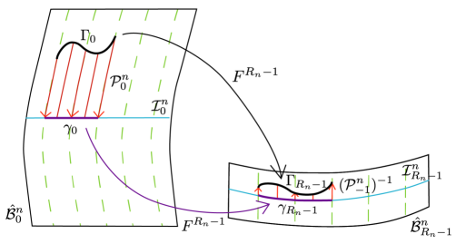
Figure 5. Projections $\mathcal{P}^{n}_{0}:\hat{\mathcal{B}}^{n}_{0}\to\mathcal{I}^{n}_{0}$ and $\mathcal{P}^{n}_{-1}:\hat{\mathcal{B}}^{n}_{R_{n}-1}\to\mathcal{I}^{n}_{R_{n}-1}$ near the critical value $v_{0}$ and critical point $v_{-1}$ respectively. On any horizontal curve $\Gamma_{0}\subset\hat{\mathcal{B}}^{n}_{0}$, the iterate $F^{R_{n}-1}$ commutes with these projections.

4.2. Passing near the critical value

Let $K_{0}\geq 1$ be the uniform constant given in (3.2). Assume that $n_{0}\leq N$ is the smallest number such that

$$\overline{K_{1}}\lambda^{\varepsilon R_{n_{0}}}<\eta,$$ (4.2)

where

$$K_{1}=K_{1}({K_{0}},\kappa_{F})\geq 1$$ (4.3)

is a uniform constant.

Let $z=(a,b)\in B_{0}=I^{h}_{0}\times I^{v}_{0}$. For $t\geq 0$, define

$$V_{z}(t):=[a-t,a+t]\times I^{v}_{0}.$$

For $p\in\hat{\mathcal{B}}^{n}_{0}$ and $t\geq 0$, denote

$$\mathcal{V}_{p}^{n}(t):=(\Psi^{n})^{-1}(V_{\Psi^{n}(p)}(t))\subset\hat{\mathcal{B}}^{n}_{0}.$$

We record the following immediate consequences of Lemmas 3.6 and 3.7, and (4.2).

Lemma 4.3.

For $n_{0}\leq n\leq N$, let $E_{p_{-1}}\in\mathbb{P}^{2}_{p_{-1}}$ be a $\lambda^{{\bar{\varepsilon}}R_{n}}$-horizontal direction at $p_{-1}\in\mathcal{B}_{-1}$. If

$$p_{0}\in\hat{\mathcal{B}}^{n}_{0}\setminus\mathcal{V}^{n}_{v_{0}}(\lambda^{{\bar{\varepsilon}}R_{n}})$$

then $E_{p_{0}}$ is $\lambda^{-{\bar{\varepsilon}}R_{n}}$-horizontal in $\hat{\mathcal{B}}^{n}_{0}$. Similarly, let $\Gamma_{-1}$ be $\lambda^{{\bar{\varepsilon}}R_{n}}$-horizontal curve in $\mathcal{B}_{-1}$. If

$$\Gamma_{0}:=F(\Gamma_{-1})\subset\hat{\mathcal{B}}^{n}_{0}\setminus\mathcal{V}^{n}_{v_{0}}(\lambda^{{\bar{\varepsilon}}R_{n}})\hskip 14.22636pt\text{with}\hskip 14.22636ptt>\lambda^{{\bar{\varepsilon}}R_{n}},$$

then $\Gamma_{0}$ is $\lambda^{-{\bar{\varepsilon}}R_{n}}$-horizontal in $C^{r}$ in $\hat{\mathcal{B}}^{n}_{0}$.

Lemma 4.4.

For $n_{0}\leq n\leq N$, let $\tilde{E}_{p_{0}}\in\mathbb{P}^{2}_{p_{0}}$ be a $\lambda^{{\bar{\varepsilon}}R_{n}}$-vertical direction at $p_{0}\in\hat{\mathcal{B}}^{n}_{0}$. If

$$p_{0}\in\hat{\mathcal{B}}^{n}_{R_{n}}\setminus\mathcal{V}^{n}_{v_{0}}(\lambda^{{\bar{\varepsilon}}R_{n}}),$$

then $\tilde{E}_{p_{0}}$ is $\lambda^{-{\bar{\varepsilon}}R_{n}}$-vertical in $\mathcal{B}_{-1}$. Similarly, let $\tilde{\Gamma}_{0}$ be $\lambda^{{\bar{\varepsilon}}R_{n}}$-vertical curve in $\hat{\mathcal{B}}^{n}_{0}$. If

$$\tilde{\Gamma}_{0}\subset\hat{\mathcal{B}}^{n}_{R_{n}}\setminus\mathcal{V}^{n}_{v_{0}}(\lambda^{{\bar{\varepsilon}}R_{n}}),$$

then $\tilde{\Gamma}_{-1}:=F^{-1}(\tilde{\Gamma}_{0})$ is $\lambda^{-{\bar{\varepsilon}}R_{n}}$-vertical in $C^{r}$ in $\mathcal{B}_{-1}$.

4.3. 1D-Like Structure

Henceforth, suppose that the combinatorics of renormalizations of $F$ are of $\mathbf{b}$-bounded type for some integer $\mathbf{b}\geq 2$. Moreover, assume that $\varepsilon$ is sufficiently small so that $\mathbf{b}{\bar{\varepsilon}}<1$. By only considering every other returns if necessary, we may also assume without loss of generality that $r_{n}:=R_{n+1}/R_{n}\geq 3$ for ${n_{0}}\leq n\leq N$.

Let $z=(a,b),w=(c,d)\in B_{0}=I^{h}_{0}\times I^{v}_{0}$. Denote

$$m:=\min\{a,c\}\hskip 14.22636pt\text{and}\hskip 14.22636ptM:=\max\{a,c\}.$$

For $t\geq 0$, define

$$V_{[z,w]}(t):=[m-t,M+t]\times I^{v}_{0}.$$

For $n_{0}\leq n\leq N$; $p,q\in\hat{\mathcal{B}}^{n}_{0}$ and $t\geq 0$, denote

$$\mathcal{V}_{[p,q]}^{n}(t):=(\Psi^{n})^{-1}(V_{[\Psi^{n}(p),\Psi^{n}(q)]}(t)).$$

Let $s\in\{0,1,2\}$. For $n_{0}\leq n\leq N-s$ and $k\geq-1$, denote

$$a^{n}_{k}:=P^{n}_{0}(v_{kR_{n}})\hskip 14.22636pt\text{and}\hskip 14.22636ptb^{n,s}_{k}:=P^{n}_{0}(v_{kR_{n}+R_{n+s}})=a^{n}_{k+R_{n+s}/R_{n}}.$$

Define

$$\hat{B}^{n,s}_{kR_{n}}:=V_{[a^{n}_{k},b^{n,s}_{k}]}(\lambda^{{\bar{\varepsilon}}R_{n}})\hskip 14.22636pt\text{and}\hskip 14.22636pt\hat{\mathcal{B}}^{n,s}_{kR_{n}}:=(\Psi^{n})^{-1}(\hat{B}^{n,s}_{kR_{n}}).$$

In particular, we have

$$\hat{\mathcal{B}}^{n}_{0}\supset\hat{\mathcal{B}}^{n,0}_{0}:=\mathcal{V}^{n}_{[v_{0},v_{R_{n}}]}(\lambda^{{\bar{\varepsilon}}R_{n}}).$$

See Figure 6.

Definition 4.5.

For $n_{0}\leq n<N$ and $1\leq s\leq N-n$, we say that the Hénon-like return $(F^{R_{n}},\Psi^{n})$ has 1D-like structure of depth $s$ if:

1. $\hat{\mathcal{B}}^{n,s}_{lR_{n}}\cap\hat{\mathcal{B}}^{n,s}_{kR_{n}}=\varnothing$ for $0\leq l,k<R_{n+s}/R_{n}$ with $l\neq k$;

2. $a^{n}_{0}=0<b^{n,s}_{0}<a^{n}_{k}\,,\,b^{n,s}_{k}<b^{n,s}_{1}<a^{n}_{1}$ for $2\leq k<R_{n+s}/R_{n}$; and

3. $F^{R_{n}}(\hat{\mathcal{B}}^{n,s}_{kR_{n}})\Subset\hat{\mathcal{B}}^{n,s}_{(k+1)R_{n}\;(\operatorname{mod}\;R_{n+s})}$ for $0\leq k<R_{n+s}/R_{n}$.

Proposition 4.6.

[Y, Proposition 6.5] Let $n_{0}\leq n\leq N$. Suppose that $F^{R_{n}}|_{\mathcal{B}^{n}_{0}}$ is twice non-trivially topological renormalizable with combinatorics of $\mathbf{b}$-bounded type. Then for $m=n-s$ with $s=O(1)$, the Hénon-like return $(F^{R_{m}},\Psi^{m})$ has 1D-like structure of depth $s$. In particular, $\hat{\mathcal{B}}^{n,0}_{0}$ is $R_{n}$-periodic.

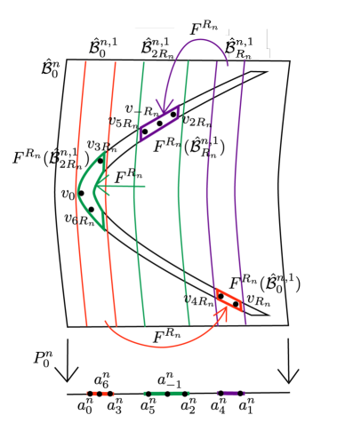
Figure 6. The 1D-like structure of depth $1$ of $(F^{R_{n}},\Psi^{n})$ for $n\geq n_{0}$ (for $r_{n}:=R_{n+1}/R_{n}=3$). The $R_{n+1}$-periodic domains $\hat{\mathcal{B}}^{n,1}_{0}$, $\hat{\mathcal{B}}^{n,1}_{R_{n}}$ and $\hat{\mathcal{B}}^{n,1}_{2R_{n}}$ containing $v_{0}$, $v_{R_{n}}$ and $v_{2R_{n}}$ respectively are vertically proper and pairwise disjoint in $\hat{\mathcal{B}}^{n}_{0}$. Moreover, $F^{R_{n}}(\hat{\mathcal{B}}^{n,1}_{kR_{n}})\Subset\hat{\mathcal{B}}^{n,1}_{(k+1)R_{n}\;(\operatorname{mod}\;R_{n+1})}$. Under the projection $P^{n}_{0}:\hat{\mathcal{B}}^{n}_{0}\to I^{n}_{0}\subset\mathbb{R}$, the orbit $\{v_{kR_{n}}\}_{k=-1}^{r_{n}}$ of the critical value are mapped to $\{a^{n}_{k}\}_{k=-1}^{r_{n}}$.

By Proposition 4.6, we may henceforth assume without loss of generality that for all $n_{0}\leq n\leq N$ such that $F^{R_{n}}|_{\mathcal{B}^{n}_{0}}$ is twice non-trivially renormalizable, we have

$$\mathcal{B}^{n}_{0}:=\hat{\mathcal{B}}^{n,0}_{0}:=\mathcal{V}^{n}_{[v_{0},v_{R_{n}}]}(\lambda^{{\bar{\varepsilon}}R_{n}}).$$ (4.4)

Lemma 4.7.

Let $n_{0}\leq n\leq N$. Suppose that $F^{R_{n}}|_{\mathcal{B}^{n}_{0}}$ is twice topological renormalizable with combinatorics of $\mathbf{b}$-bounded type. For $s\in\{1,2\}$ and $m:=n-s$, let $\Gamma_{0}$ be a $\lambda^{-{\bar{\varepsilon}}R_{m}}$-horizontal curve in $\mathcal{B}^{n}_{0}$. Then the following statements hold for $1\leq k\leq R_{n}/R_{m}$:

1. $\Gamma_{(k-1)R_{m}}$ is $\lambda^{-{\bar{\varepsilon}}R_{m}}$-horizontal in $\mathcal{B}^{m}_{0}$; and

2. $\Gamma_{kR_{m}-1}$ is $\lambda^{(1-{\bar{\varepsilon}})R_{m}}$-horizontal in $\mathcal{B}_{-1}$.

Proof.

The result is an immediate consequence of Lemmas 4.1 iii) and 4.3, and Proposition 4.6. ∎

5. Critical Recurrence

Let $F$ be the infinitely regularly Hénon-like renormalizable map with combinatorics of bounded type considered in Subsection 4.3 (with $N=\infty$). In this section, we prove the following result.

Theorem 5.1.

We have

$$\mathcal{Z}_{0}:=\bigcap_{n=1}^{\infty}\mathcal{B}^{n}_{R_{n}}=\{v_{0}\}.$$

Consequently, the orbit of $v_{0}$ is recurrent.

Proof.

Let

$$\mathcal{Y}_{0}:=\bigcap_{n=1}^{\infty}\mathcal{B}^{n}_{0},\hskip 14.22636pt\mathcal{I}^{\infty}_{0}:=\mathcal{I}^{h}_{0}\cap\mathcal{Y}_{0}\hskip 14.22636pt\text{and}\hskip 14.22636ptI^{\infty}_{0}:=\pi_{h}\circ\Phi_{0}(\mathcal{I}^{\infty}_{0}).$$

Note that every point $p_{0}\in\mathcal{Y}_{0}$ is infinitely forward $(L,\varepsilon,\lambda)$-regular. Moreover, arguing as in the proof of Proposition 3.2, we see that $W^{ss}(p_{0})$ is vertically proper in $\mathcal{B}^{1}_{0}$. Let $W^{ss}_{\operatorname{loc}}(p_{0})$ be the connected component of $W^{ss}(p_{0})\cap\mathcal{B}^{1}_{0}$ containing $p_{0}$. Then we have

$$\mathcal{Y}_{0}=\bigcup_{p_{0}\in\mathcal{I}^{\infty}_{0}}W^{ss}_{\operatorname{loc}}(p_{0}).$$

Since $\mathcal{Y}_{i}:=F^{i}(\mathcal{Y}_{0})\subset\mathcal{B}^{n}_{i}$ for all $n\in\mathbb{N}$ such that $0\leq i<R_{n}$, we see that

$$\mathcal{Y}_{i}\cap\mathcal{Y}_{0}=\varnothing\hskip 14.22636pt\text{for}\hskip 14.22636pti\in\mathbb{N}.$$

We claim that $\mathcal{Y}_{0}=W^{ss}_{\operatorname{loc}}(v_{0})$. Suppose towards a contradiction that this is not true. By (3.7) and (3.11), this means that there exists a uniform constant $b>0$ such that $(0,b)\subset I^{\infty}_{0}$.

Recall that for $n\in\mathbb{N}$, the curve $\mathcal{I}^{n}_{R_{n}}$ is vertical quadratic in $\mathcal{B}^{n}_{0}$. Let $c^{n}_{0}\in\mathcal{I}^{n}_{0}$ be the unique point such that

$$E^{gv}_{\Psi^{n}\left(c^{n}_{R_{n}}\right)}=D(\Psi^{n}\circ F^{R_{n}})\left(E^{h}_{c^{n}_{0}}\right).$$

By Theorem 3.5 ii), we see that $\Phi_{-1}(\mathcal{I}^{n}_{R_{n}-1})$ is $\lambda^{(1-{\bar{\varepsilon}})R_{n}}$-horizontal in $\mathcal{B}_{-1}$. Hence, by Theorem 3.5 i), we have

$$\|c^{n}_{R_{n}}-v_{0}\|<\lambda^{(1-{\bar{\varepsilon}})R_{n}}.$$

Let $M\in\mathbb{N}$ be sufficiently large so that for $n\geq M$, we have

$$P^{n}_{0}(c^{n}_{R_{n}})<\lambda^{(1-{\bar{\varepsilon}})R_{n}}<\lambda^{{\bar{\varepsilon}}R_{M}}<b/2.$$

Note that for $0\leq k<R_{n}/R_{M}$, we have

$$\mathcal{B}^{n}_{kR_{M}}\cap\mathcal{B}^{n}_{0}=\varnothing.$$

Thus, applying Lemma 4.3 and proceeding by induction, we see that the curve $\mathcal{I}^{n}_{kR_{M}}$ is $\lambda^{-{\bar{\varepsilon}}R_{M}}$-horizontal in $\mathcal{B}^{M}_{0}$, and $\mathcal{I}^{n}_{(k+1)R_{M}-1}$ is $\lambda^{(1-{\bar{\varepsilon}})R_{M}}$-horizontal in $\mathcal{B}_{-1}$.

Define $\mathcal{B}^{n}_{-kR_{M}}$ for $0\leq k<R_{n}/R_{M}$ inductively as follows. Suppose that

• $F^{kR_{M}}(\mathcal{B}^{n}_{kR_{M}})\Subset\mathcal{B}^{n}_{0}$;

• $\Psi^{M}(\mathcal{B}^{n}_{-kR_{M}})$ is a vertically proper quadrilateral in $B^{M}_{0}$, whose side boundaries are $\lambda^{(1-{\bar{\varepsilon}})R_{M}}$-vertical; and

• $\mathcal{B}^{n}_{-kR_{M}}\supset\mathcal{I}^{n}_{R_{n}-kR_{M}}$.

Since $\mathcal{B}^{n}_{0}$ is $R_{n}$-periodic (see Proposition 4.6 iii)), property i) implies that

$$\mathcal{B}^{n}_{-kR_{M}}\cap\mathcal{B}^{n}_{-iR_{M}}=\varnothing\hskip 14.22636pt\text{for}\hskip 14.22636pt0\leq i<k.$$

This, together with property ii) ensure that

$$F^{-1}(\mathcal{B}^{n}_{-kR_{M}})\cap\mathcal{B}^{M}_{R_{M}-1}$$

consists of exactly two connected components (unless $k=0$, in which case there is only one connected component). Let $\mathcal{B}^{n}_{-kR_{M}-1}$ be the component containing $\mathcal{I}^{n}_{R_{n}-kR_{M}-1}$. Define

$$\mathcal{B}^{n}_{-(k+1)R_{M}}:=F^{-R_{M}+1}(\mathcal{B}^{n}_{-kR_{M}-1}).$$

By Lemma 4.4, we see that

$$\partial\mathcal{B}^{n}_{-kR_{M}-1}\setminus\partial\mathcal{B}^{M}_{R_{M}-1}$$

consists of two $\lambda^{-{\bar{\varepsilon}}R_{M}}$-vertical curves $\Gamma^{n,\pm}_{-kR_{M}-1}$ in $\mathcal{B}_{-1}$, and

$$\Gamma^{n,\pm}_{-(k+1)R_{M}}:=F^{-R_{M}+1}(\Gamma^{n,\pm}_{-kR_{M}-1})$$

are $\lambda^{(1-{\bar{\varepsilon}})R_{M}}$-vertical and vertically proper in $\mathcal{B}^{M}_{0}$.

Since the sets

$$\mathcal{B}^{n}_{-(k+1)R_{M}}\supset\mathcal{I}^{n}_{R_{n}-(k+1)R_{M}}\hskip 14.22636pt\text{for}\hskip 14.22636pt0\leq k<R_{n}/R_{M}$$

are disjoint, the intervals

$$I^{n}_{kR_{M}}:=P^{M}_{0}(\mathcal{I}^{n}_{kR_{M}})$$

must be disjoint in $I^{M}_{0}$.

Consider the diffeomorphism $h_{M}$ given in Theorem 3.5 ii). Define

$$g_{k}^{n}(x):=\mathcal{P}^{M}_{0}\circ F\circ(\mathcal{P}^{M}_{-1}|_{\mathcal{I}^{n}_{(k+1)R_{M}-1}})^{-1}(h_{M}(x),0)\hskip 14.22636pt\text{for}\hskip 14.22636ptx\in I^{n}_{kR_{M}}.$$

Since $\mathcal{I}^{n}_{(k+1)R_{M}-1}$ and $\mathcal{I}^{n}_{(k+1)R_{M}}$ are uniformly horizontal in $\mathcal{B}_{-1}$ and $\mathcal{B}_{0}$ respectively, it follows that $\|g_{k}^{n}\|_{C^{r}}$ is uniformly bounded. Moreover,

$$\sum_{k=0}^{R_{n}/R_{M}-1}|I^{n}_{kR_{M}}|<|I^{M}_{0}|.$$

Thus, we conclude from Theorem B.1 that

$$G^{n}:=g_{R_{n}/R_{M}-1}^{n}\circ\ldots\circ g_{0}^{n}$$

has uniformly bounded distortion.

Let

$$I^{n+1}_{-R_{n}}=P^{M}_{0}(\mathcal{B}^{n+1}_{-R_{n}}).$$

Then $I^{n+1}_{-R_{n}}$ and $I^{n+1}_{0}$ are disjoint intervals in $I^{n}_{0}$. Moreover, $|I^{n+1}_{0}|$ is uniformly bounded below, while

$$|I^{n+1}_{-R_{n}}|,|I^{n+1}_{R_{n}}|\to 0\hskip 14.22636pt\text{as}\hskip 14.22636ptn\to\infty.$$

However,

$$G^{n}(I^{n+1}_{-R_{n}})=I^{n+1}_{0}\hskip 14.22636pt\text{and}\hskip 14.22636ptG^{n}(I^{n+1}_{0})=I^{n+1}_{R_{n}}.$$

This contradicts the fact that $G^{n}$ has uniformly bounded distortion. The result follows. ∎

6. A Priori Bounds

Let $r\geq 2$ be an integer, and consider a $C^{r+4}$-Hénon-like map $F:B\to B$. For some $N\in\mathbb{N}\cup\{\infty\}$; $L\geq 1$ and $\varepsilon,\lambda\in(0,1)$, suppose that $F$ has $N$ nested $(L,\varepsilon,\lambda)$-regular Hénon-like returns given by (1.2) with combinatorics of $\mathbf{b}$-bounded type for some integer $\mathbf{b}\geq 3$. By only considering every other returns if necessary, we may also assume without loss of generality that $r_{n}:=R_{n+1}/R_{n}\geq 3$ for ${n_{0}}\leq n\leq N$. Assume that $\varepsilon$ is sufficiently small so that $\mathbf{b}{\bar{\varepsilon}}<1$. Also assume that $N$ is sufficiently large, so that for some smallest number $0\leq n_{0}\leq N$, we have (4.2). Lastly, suppose that $F^{R_{N}}|_{\mathcal{B}^{N}_{0}}$ is twice non-trivially topologically renormalizable (so that the Hénon-like returns of $F$ have 1D-like structure of depth $2$ by Proposition 4.6).

6.1. The outline of strategy

For $n_{0}\leq n\leq N$, consider the horizontal cross-section of the $n$th renormalization domain $\mathcal{B}^{n}_{0}$:

$$\mathcal{I}^{n}_{0}:=(\Psi^{n})^{-1}(I^{n}_{0}\times\{0\})=\mathcal{I}^{h}_{0}\cap\mathcal{B}^{n}_{0}\ni v_{0}.$$

See (3.10). We want to prove that $\operatorname{Dis}(F^{R_{n}},\mathcal{I}^{n}_{0})$ is uniformly bounded.

The general strategy is to reduce the 2D dynamics of $F$ acting on $\mathcal{I}^{n}_{0}$ to a 1D mapping scheme for which standard 1D arguments can be applied to control distortion. Below we give a broad description of this 1D mapping scheme using simpler notations to better convey the main ideas. In the actual proof, the 1D scheme is derived from the 2D dynamics it is modeling, which forces the notations to become more complicated.

Fix some intervals $I_{0},I_{-1}\subset\mathbb{R}$. For $1\leq n\leq N$, let $\{A^{n}_{i}\}_{i=0}^{R_{n}-1}$ and $\{{\check{A}}^{n}_{i}\}_{i=0}^{R_{n}-1}$ be collections of pairwise disjoint subintervals in $I_{0}$ and $I_{-1}$ respectively so that $0\in{\check{A}}^{n}_{R_{n}-1}\subset I_{-1}$. Consider the following mapping scheme for $1\leq i\leq R_{n}$:

• a $C^{2}$-diffeomorphism

  $$\phi^{n}_{i}:A^{n}_{i-1}\to{\check{A}}^{n}_{i-1}:=\phi^{n}_{i}(A^{n}_{i-1})$$

  with uniformly bounded $C^{2}$-norm; and

• a quadratic power map

  $$g^{n}_{i}:{\check{A}}^{n}_{i-1}\to A^{n}_{i}:=g^{n}_{i}({\check{A}}^{n}_{i-1})$$

  given by

  $$g^{n}_{i}(x)=x^{2}+a^{n}_{i}\hskip 14.22636pt\text{for some}\hskip 14.22636pta^{n}_{i}\in\mathbb{R}.$$

Define

$$H_{i}:=\phi^{n}_{i}\circ g^{n}_{i-1}\circ\phi^{n}_{i-1}\circ\ldots\circ g^{n}_{1}\circ\phi^{n}_{1}.$$

Suppose that the domains of $\phi^{n}_{i}$ for $1\leq i\leq R_{n}$ can be extended so that $g^{n}_{i}\circ H_{i}$ maps a strictly larger interval $\tilde{A}^{n}_{0,i}\Supset A^{n}_{0}$ diffeomorphically onto an image $g^{n}_{i}\circ H_{i}(\tilde{A}^{n}_{0,i})$ that contains the two adjacent neighbors $A^{n}_{\iota_{-}(i)}$ and $A^{n}_{\iota_{+}(i)}$ of $A^{n}_{i}$ (or at least subintervals in $A^{n}_{\iota_{\pm}(i)}$ of commensurate lengths). Then we can apply Koebe distortion theorem (see Section B) to conclude that $H_{R_{n}}|_{A^{n}_{0}}$ has uniformly bounded distortion.

We now give a brief description of how the 2D dynamics of $F$ acting on the curve $\mathcal{I}^{n}_{0}$ is reduced to the above 1D mapping scheme. The main idea is to weave into the dynamics of $F$ systematic applications of projections near the critical value $v_{0}$. This confines the orbit of $\mathcal{I}^{n}_{0}$ to lie in a fixed union of curves $\{\mathcal{I}^{n_{0}}_{i}\}_{i=0}^{R_{n_{0}}-1}$. These projections are then “undone” near the critical point $v_{-1}$ to recover the original dynamics. See the definitions of the maps $H^{n}_{i}$ and $\hat{H}_{i}$, as well as Lemmas 6.2 and 6.3. See also Figure 7.

The pairwise disjointedness of the collection of images $\{\mathcal{J}^{n}_{i}\}_{i=0}^{R_{n}-1}$ of $\mathcal{I}^{n}_{0}$ under $\hat{H}_{i}$ relies on the 1D combinatorial structures of the renormalizations of the 2D map $F$ established in Section 4.3. See Figure 6 and Lemma 6.10.

Contributions by quadratic power maps in the composition $\hat{H}_{i}$ arise in the following way. When the inverse projection is applied near the critical point $v_{-1}$, it is onto a nearly horizontal curve (approximating a subarc of a center manifold of $v_{-1}$). Under one iterate of $F$, this curve is mapped to a subarc of a vertical quadratic curve near the critical value $v_{0}$. Then projecting along a vertical foliation to the transverse horizontal arc $\mathcal{I}^{n_{0}}_{0}\supset\mathcal{I}^{n}_{0}$ produces the effect of applying a quadratic power map. See Proposition 6.18.

Lastly, the extension of $\hat{H}_{i}$ to a strictly larger domain $\tilde{\mathcal{I}}^{n}_{0,i}\Supset\mathcal{I}^{n}_{0}$ so that the image $\hat{H}_{i}(\tilde{\mathcal{I}}^{n}_{0,i})$ covers (commensurate portions of) the adjacent neighbors $\mathcal{J}^{n}_{\iota_{\pm}(i)}$ of $\mathcal{J}^{n}_{i}$ is done in Propositions 6.14 and 6.17.

6.2. The proof of the Main Theorem

First, we need the following lemma (which requires the 3 additional degrees of smoothness assumed in this section). Recall that $P^{n}_{0}:=\pi_{h}\circ\Psi^{n}$ for $n_{0}\leq n\leq N$.

Lemma 6.1.

Let $\kappa_{F},K_{1}>0$ be the constants given in Theorem 3.5 and (4.3) respectively. Consider a $C^{r+3}$-map $g:I\to\mathbb{R}$ on an interval $I\subset I^{h}_{-1}$ such that $\|g\|_{C^{2}}<\underline{\kappa_{F}}$. Denote $G(x):=(x,g(x)).$ Then there exist $a\in I^{h}_{0}$ and a $C^{r}$-diffeomorphism $\psi:I\to\psi(I)$ with

$$\|\psi^{\pm 1}\|_{C^{r}}<K_{1}(1+\|g\|_{C^{r+3}})$$

such that we have

$$Q(x):=P^{n}_{0}\circ F\circ\Phi_{-1}^{-1}\circ G(x)=\kappa_{F}\cdot(\psi(x))^{2}+a$$ (6.1)

where defined.

Proof.

By Theorem 3.5 i), it suffices to show that there exists $\tilde{\psi}_{g}$ with

$$\|\tilde{\psi}^{\pm 1}\|_{C^{r}}<{K_{1}}(1+\|g\|_{C^{r+3}})$$

such that

$$\tilde{Q}(x):=\pi_{h}\circ\Phi_{0}\circ F\circ\Phi_{-1}^{-1}\circ G(x)=\kappa_{F}\cdot(\tilde{\psi}(x))^{2}+\tilde{a}.$$

By (3.7), we have $\tilde{Q}=f_{0}-\lambda\cdot g.$ By the bound on $\|g\|_{C^{2}}$, we see that $\tilde{Q}$ has a unique critical point, $\tilde{Q}^{\prime\prime}(x)$ is bounded below by $c\kappa_{F}$ for some uniform constant $c>0$, and

$$\|\tilde{Q}^{\prime\prime}\|_{C^{r+1}}<{K_{1}}(1+\|g\|_{C^{r+3}}).$$

The result now follows from Lemma C.3. ∎

For $n_{0}\leq n\leq N$, define a sequence of maps $\{H^{n}_{i}\}_{i=0}^{\infty}$ as follows. First, let $H^{n_{0}}_{i}:=F^{i}.$ Proceeding inductively, suppose $H^{n-1}_{i}$ is defined. Write $i=j+kR_{n}$ with $k\geq 0$ and $0\leq j<R_{n}$. Define

$$H^{n}_{i}:=H^{n-1}_{j}\circ\mathcal{P}^{n}_{0}\circ F^{kR_{n}},$$

where

$$\mathcal{P}^{n}_{0}:=(\Psi^{n})^{-1}\circ\Pi_{h}\circ\Psi^{n}$$

is the $n$th projection map near the critical value $v_{0}$. Observe that $H^{n}_{i}$ is well-defined on $\mathcal{B}^{n}_{0}$.

Lemma 6.2.

Let $s\in\{1,2\}$ and $n_{0}\leq n\leq N-s$. Then $H^{n}_{i}|_{\mathcal{I}^{n+s}_{1}}$ is a diffemorphism for $0\leq i<R_{n+s}$.

Proof.

The statement is clearly true for $n={n_{0}}$. Suppose the statement is true for $n-1$. If $i<R_{n}$, then

$$H^{n}_{i}|_{\mathcal{I}^{n+s}_{1}}=H^{n-1}_{i}|_{\mathcal{I}^{n+s}_{1}}$$

is a diffeomorphism. Suppose the same is true for $i<(k-1)R_{n}$ with $2\leq k<R_{n+s}/R_{n}$. Observe that

$$H^{n}_{kR_{n}}=\mathcal{P}^{n}_{0}\circ F^{kR_{n}}.$$

By Lemma 4.7 i), the map $\mathcal{P}^{n}_{0}|_{\mathcal{I}^{n+s}_{kR_{n}}}$ is a diffeomorphism. For $i=j+kR_{n}$ with $j<R_{n}$, we have

$$H^{n}_{i}:=H^{n-1}_{j}\circ\mathcal{P}^{n}_{0}\circ F^{kR_{n}}.$$

Since

$$\mathcal{P}^{n}_{0}(\mathcal{I}^{n+s}_{kR_{n}})\subset\mathcal{I}^{n}_{0},$$

the result follows. ∎

Recall the definition of $\mathcal{P}^{n}_{-1}$ for $n_{0}\leq n\leq N$ given in (4.1).

Lemma 6.3.

For $s\in\{1,2\}$ and $n_{0}\leq n\leq N-s$, let $\Gamma_{0}$ be a $C^{r}$-curve which is $\lambda^{-{\bar{\varepsilon}}R_{n}}$-horizontal in $\mathcal{B}^{n+s}_{0}$. Then for $1\leq k\leq R_{n+s}/R_{n}$, we have

$$F^{kR_{n}-1}|_{\Gamma_{0}}=\left(\mathcal{P}^{n_{0}}_{-1}|_{\Gamma_{kR_{n}-1}}\right)^{-1}\circ H^{n}_{kR_{n}-1}|_{\Gamma_{0}}.$$

Proof.

If $k=1$, then the result follows immediately from Lemma 4.2. Suppose the result is true for some $n_{0}\leq n<N-s$ and $1\leq k<R_{n+s}/R_{n}$. By definition, we have

$$H^{n}_{(k+1)R_{n}-1}=H^{n}_{kR_{n}-1}\circ F^{R_{n}}.$$

If $\Gamma_{0}$ is a $C^{r}$-curve which is $\lambda^{-{\bar{\varepsilon}}R_{n}}$-horizontal in $\mathcal{B}^{n+s}_{0}$, then by Lemma 4.7 i), we see that $\Gamma_{R_{n}}:=F^{R_{n}}(\Gamma_{0})$ is a $C^{r}$-curve which is $\lambda^{-{\bar{\varepsilon}}R_{n}}$-horizontal in $\mathcal{B}^{n}_{0}$. Thus, by induction, we have

$$F^{kR_{n}-1}|_{\Gamma_{R_{n}}}=\left(\mathcal{P}^{n_{0}}_{-1}|_{\Gamma_{(k+1)R_{n}-1}}\right)^{-1}\circ H^{n}_{kR_{n}-1}|_{\Gamma_{R_{n}}}.$$

Composing on the right by $F^{R_{n}}|_{\Gamma_{0}}$, the result is true in this case.

Finally, suppose that the result is true for some $n_{0}\leq n<N-s$ and $k=R_{n+1}/R_{n}$. Let $\gamma_{0}:=\mathcal{P}^{n+1}_{0}(\Gamma_{0})$. By the induction hypothesis, we have:

$$F^{R_{n+1}-1}|_{\gamma_{0}}=\left(\mathcal{P}^{n_{0}}_{-1}|_{\gamma_{R_{n+1}-1}}\right)^{-1}\circ H^{n}_{R_{n+1}-1}|_{\gamma_{0}}.$$

Applying Lemma 4.2:

$$F^{R_{n+1}-1}|_{\Gamma_{0}} =\left(\mathcal{P}^{n+1}_{-1}|_{\Gamma_{R_{n+1}-1}}\right)^{-1}\circ\left(\mathcal{P}^{n_{0}}_{-1}|_{\gamma_{R_{n+1}-1}}\right)^{-1}\circ H^{n}_{R_{n+1}-1}\circ\mathcal{P}^{n+1}_{0}|_{\Gamma_{0}}$$

$$=\left(\mathcal{P}^{n_{0}}_{-1}|_{\Gamma_{R_{n+1}-1}}\right)^{-1}\circ H^{n+1}_{R_{n+1}-1}|_{\Gamma_{0}}.$$

∎

Figure 7. Visualization of the map $H^{n_{0}}_{i}$ for $0\leq i<R_{n_{0}+1}$ acting on the horizontal curve $\mathcal{I}^{n_{0}+1}_{0}\subset\mathcal{I}^{n_{0}}_{0}$ (for $r_{n_{0}}:=R_{n_{0}+1}/R_{n_{0}}=3$). The orbit of $\mathcal{I}^{n_{0}+1}_{0}$ makes returns to $\mathcal{B}^{n_{0}}_{0}\ni v_{0}$ under $F^{kR_{n}}$ for $0\leq k<r_{n_{0}}$. At these moments, the projection map $\mathcal{P}^{n_{0}}_{0}$ is applied to $\mathcal{I}^{n_{0}+1}_{kR_{n_{0}}}$ to bring it down to $\mathcal{I}^{n_{0}}_{0}$. These projections are then “undone” in $\mathcal{B}^{n_{0}}_{R_{n_{0}}-1}\ni v_{-1}$ to return to $\mathcal{I}^{n_{0}+1}_{(k+1)R_{n_{0}-1}}$. For $n>n_{0}$, the multiple projections (at various depths) can be applied to the orbit of $\mathcal{I}^{n}_{0}$ near $v_{0}$ before they are undone near $v_{-1}$.

We also define another sequence of maps $\{\hat{H}_{i}\}_{i=0}^{R_{N}-1}$ as follows (if $N=\infty$, then $R_{N}=\infty$). If $i<2R_{n_{0}}$, let $\hat{H}_{i}:=F^{i}.$ Otherwise, let $n_{0}\leq n<N$ be the largest number such that $i\geq 2R_{n}$, and define $\hat{H}_{i}:=H^{n}_{i}.$ Observe that by Lemma 6.3, we have

$$\hat{H}_{R_{n}-1}|_{\mathcal{I}^{n}_{0}}=H^{n-1}_{R_{n}-1}|_{\mathcal{I}^{n}_{0}}=\mathcal{P}^{n_{0}}_{-1}|_{\mathcal{I}^{n}_{R_{n}-1}}\circ F^{R_{n}-1}|_{\mathcal{I}^{n}_{0}}.$$ (6.2)

Remark 6.4.

In the definition of $\hat{H}_{i}:=H^{n}_{i}$, we set $n$ to be the largest number such that $i\geq 2R_{n}$ rather than $i\geq R_{n}$ for the following technical reason. Observe that

$$H^{n}_{R_{n}}(\mathcal{I}^{n+1}_{0})=\mathcal{P}^{n}_{0}(\mathcal{I}^{n+1}_{R_{n}}).$$

The domain of $\mathcal{P}^{n}_{0}$ is equal to $\mathcal{B}^{n}_{0}$, whose right vertical boundary is $\lambda^{{\bar{\varepsilon}}R_{n}}$ distance away from $\mathcal{I}^{n+1}_{R_{n}}$. Hence, $H^{n}_{R_{n}}|_{\mathcal{I}^{n+1}_{0}}$ does not extend to a horizontal curve $\tilde{\mathcal{I}}^{n+1}_{0,i}$ substantially larger than $\mathcal{I}^{n+1}_{0}$ (so that its image would cover the adjacent neighbors of $H^{n}_{R_{n}}(\mathcal{I}^{n+1}_{0})$), since if it did, then $F^{R_{n}}(\tilde{\mathcal{I}}^{n+1}_{0,i})$ would lie outside of the domain $\mathcal{B}^{n}_{0}$ of $\mathcal{P}^{n}_{0}$.

The remainder of the section is devoted to the proof of the following theorem, whose corollary immediately implies the Main Theorem.

Theorem 6.5.

There exists a uniform constant

$$\mathbf{K}=\mathbf{K}(L,\lambda,\varepsilon,\lambda^{1-\varepsilon}\|DF^{-1}\|,\|DF\|_{C^{5}},\|F^{R_{n_{0}}}|_{\mathcal{B}^{n_{0}}}\|_{C^{6}},\kappa_{F})\geq 1$$

such that for all $n_{0}\leq n\leq N$, we have

$$\operatorname{Dis}(\hat{H}_{i},\mathcal{I}^{n}_{0})<\mathbf{K}\hskip 14.22636pt\text{for}\hskip 14.22636pt0\leq i<R_{n}.$$

Corollary 6.6.

For $n_{0}\leq n\leq N$, let $h_{n}:I^{n}_{0}\to h_{n}(I^{n}_{0})$ be the diffeomorphism given in Theorem 3.5 ii). Then $\operatorname{Dis}(h_{n},I^{n}_{0})<\mathbf{K}$, where $\mathbf{K}>1$ is the uniform constant given in Theorem 6.5.

Observe that any number $2R_{n_{0}}\leq i<R_{N}$ can be uniquely expressed as

$$i=j+a_{n_{0}}R_{n_{0}}+a_{n_{0}+1}R_{n_{0}+1}+\ldots+a_{n}R_{n}$$

for some $n_{0}\leq n<N$, where

1. $0\leq j<R_{n_{0}}$;

2. $0\leq a_{m}<r_{m}$ for ${n_{0}}\leq m<n$; and

3. $2\leq a_{n}<2r_{n}$.

In this case, we denote

$$i:=j+[a_{n_{0}},a_{n_{0}+1},\ldots,a_{n}].$$

We extend this notation to $i<2R_{n_{0}}$ by writing

$$i=j+[a_{n_{0}}]\hskip 14.22636pt\text{for some}\hskip 14.22636pta_{n_{0}}\in\{0,1\}$$

We record the following easy observation.

Lemma 6.7.

Let $2R_{n_{0}}\leq i<R_{N}$ be given by

$$i=j+[a_{n_{0}},\ldots,a_{n}].$$

Then we have

$$\hat{H}_{i}=H^{n}_{i}=F^{j}\circ\left(\mathcal{P}^{n_{0}}_{0}\circ F^{a_{n_{0}}R_{n_{0}}}\right)\circ\ldots\circ\left(\mathcal{P}^{n}_{0}\circ F^{a_{n}R_{n}}\right).$$

For $n_{0}\leq n\leq N$, we define a collection of arcs $\{\mathcal{J}^{n}_{i}\}_{i=0}^{R_{n}-1}$ by

$$\mathcal{J}^{n}_{i}:=\hat{H}_{i}(\mathcal{I}^{n}_{0})\hskip 14.22636pt\text{for}\hskip 14.22636pt0\leq i<R_{n}.$$ (6.3)

See Figure 8.

Lemma 6.8.

Let $n_{0}\leq n\leq N$ and $0\leq i<R_{n}$. If

$$i=[0,\ldots,0,a_{m},a_{m+1},\ldots,a_{k}]$$

for some ${n_{0}}\leq m\leq k<n$, then we have $\mathcal{J}^{n}_{i}\subset\mathcal{I}^{m}_{0}.$ Moreover, we have

$$\mathcal{J}^{n}_{i+l}=H^{m-1}_{l}(\mathcal{J}^{n}_{i})\hskip 14.22636pt\text{for}\hskip 14.22636pt0\leq l<R_{m}.$$

Proof.

Observe that

$$\mathcal{P}^{k}_{1}\circ F^{a_{k}R_{k}}(\mathcal{I}^{k+1}_{1})\subset\mathcal{I}^{k}_{1}.$$

By Lemma 6.7, the result follows from induction. ∎

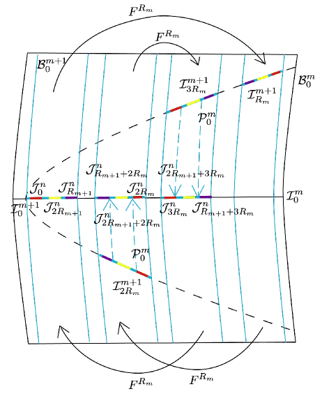
Figure 8. Arcs $\mathcal{J}^{n}_{i}:=\hat{H}_{i}(\mathcal{I}^{n}_{0})$ with $0\leq i<R_{n}$ that are contained in $\mathcal{I}^{m}_{0}$ for some $m<n$. For $0\leq k<r_{m+1}$, we have $\mathcal{J}^{n}_{kR_{m+1}}\subset\mathcal{I}^{m+1}_{0}$. For $2\leq l<r_{m}$, we have $\mathcal{J}^{n}_{kR_{m+1}+lR_{m}}=\mathcal{P}^{m}_{0}\circ F^{R_{m}}(\mathcal{J}^{n}_{kR_{m+1}})$.

Lemma 6.9.

For $n_{0}\leq n\leq N$ and $0\leq i<R_{n}$, we have $\mathcal{J}^{n}_{i}\subset\mathcal{I}^{n_{0}}_{i\;(\operatorname{mod}\;R_{n_{0}})}.$

Proof.

The result follows immediately from Lemma 6.8. ∎

Let $\Gamma:[0,1]\to\mathbb{R}^{2}$ be a parameterized Jordan arc. For

$$0\leq a<b<c<d\leq 1,$$

consider the subarcs $\Gamma_{1}:=\Gamma(a,b)$ and $\Gamma_{2}:=\Gamma(c,d)$ of $\Gamma$. We denote $\Gamma_{1}<_{\Gamma}\Gamma_{2}.$ Let $\Gamma_{3}$ be another subarc of $\Gamma$. We denote $\Gamma_{1}\leq_{\Gamma}\Gamma_{3}$ if either $\Gamma_{1}<_{\Gamma}\Gamma_{3}$ or $\Gamma_{1}=\Gamma_{3}.$

Henceforth, we consider $\mathcal{I}^{n_{0}}_{0}$ with parameterization given by

$$\mathcal{I}^{n_{0}}_{0}(t):=(\Psi^{n_{0}})^{-1}(t,0)\hskip 14.22636pt\text{for}\hskip 14.22636ptt\in I^{n_{0}}_{0}.$$

Note that $\mathcal{I}^{n_{0}}_{0}\circ P^{n_{0}}_{0}=\mathcal{P}^{n_{0}}_{0}.$ Moreover,

$$P^{n_{0}}_{0}(v_{0})=0<P^{n_{0}}_{0}(v_{R_{n_{0}}}).$$

Lemma 6.10.

For $s\in\{1,2\}$; $n_{0}\leq n\leq N-s$ and $1<k<R_{n+s}/R_{n}$, we have

$$\mathcal{J}^{n+s}_{0}<_{\mathcal{I}^{n_{0}}_{0}}\mathcal{J}^{n+s}_{kR_{n}}<_{\mathcal{I}^{n_{0}}_{0}}\mathcal{J}^{n+s}_{R_{n}}.$$

Proof.

Observe that

• For $s\in\{1,2\}$:

  $$\mathcal{J}^{n+s}_{R_{n}}=H^{n-1}_{R_{n}}(\mathcal{I}^{n+s}_{0})=\mathcal{P}^{n-1}_{0}\circ F^{R_{n}}(\mathcal{I}^{n+s}_{0}).$$

• For $1<k<sr_{n}$:

  $$\mathcal{J}^{n+s}_{kR_{n}}=H^{n}_{kR_{n}}(\mathcal{I}^{n+s}_{0})=\mathcal{P}^{n}_{0}\circ F^{kR_{n}}(\mathcal{I}^{n+s}_{0}).$$

In the case $s=1$, and the case $s=2$ and $1<k<2r_{n}$ follow immediately from Proposition 4.6.

Replacing $n$ by $n+1$ and applying the above conclusion, we see that for $1<l<r_{n+1}$:

$$\mathcal{J}^{n+2}_{0}<_{\mathcal{I}^{n_{0}}_{0}}\mathcal{J}^{n+2}_{lR_{n+1}}<_{\mathcal{I}^{n_{0}}_{0}}\mathcal{J}^{n+2}_{R_{n+1}}.$$

Note that for $2<k<r_{n}$:

$$\mathcal{J}^{n+2}_{lR_{n+1}+kR_{n}}=H^{n}_{kR_{n}}|_{\mathcal{I}^{n+1}_{0}}(\mathcal{J}^{n+2}_{lR_{n+1}}).$$

The result now follows from Lemma 6.2. ∎

Let $\Gamma_{0}:[0,|\Gamma_{0}|]\to\mathbb{R}^{2}$ be a $C^{1}$-curve parameterized by its arclength. Let $\Gamma_{1}:=\Gamma_{0}(l,|\Gamma_{0}|-l)$ for some $0<l<|\Gamma_{0}|/2$ be a subarc of $\Gamma_{0}$. We denote $\Gamma_{1}=\Gamma_{0}[-l]$ and $\Gamma_{0}=\Gamma_{1}[+l]$. Let $\Gamma_{2}$ be a $C^{1}$-curve such that $\Gamma_{1}\subset\Gamma_{2}\subset\Gamma_{0}$. We denote

$$\Gamma_{0}\{-l\}=\Gamma_{2}=\Gamma_{1}\{+l\}.$$

Lastly, if $\Gamma_{3}$ and $\Gamma_{4}$ are $C^{1}$-curves in $\mathbb{R}^{2}$ and we have $\Gamma_{3}[-l]\subset\Gamma_{4}\subset\Gamma_{3}[+l],$ then we denote $\Gamma_{4}=\Gamma_{3}\{\sim l\}.$ See Figure 9. These notations can be extended to intervals in $\mathbb{R}$ in the obvious way.

Figure 9. Illustration of the relations between $\Gamma_{0}=\Gamma_{1}[+l]$, $\Gamma_{1}=\Gamma_{0}[-l]$, $\Gamma_{0}\{-l\}=\Gamma_{2}=\Gamma_{1}\{+l\}$ (above); and $\Gamma_{3}$ and $\Gamma_{4}=\Gamma_{3}\{\sim l\}$ (below).

Let ${n_{0}}<n\leq N$, and consider the collection of arcs $\{\mathcal{J}^{n}_{i}\}_{i=0}^{R_{n}-1}$. By Lemma 6.9 and Lemma 6.10, for $2R_{n_{0}}\leq i<R_{n}$, there exist unique numbers $0\leq\iota^{n}_{-}(i),\iota^{n}_{+}(i)<R_{n}$ such that

$$\iota^{n}_{\pm}(i)=i\;(\operatorname{mod}\;R_{n_{0}}),$$

and the arcs $\mathcal{J}^{n}_{\iota^{n}_{-}(i)}$ and $\mathcal{J}^{n}_{\iota^{n}_{+}(i)}$ are the two nearest neighbors of $\mathcal{J}^{n}_{i}$ (one on each side) in $\mathcal{I}^{n_{0}}_{i\;(\operatorname{mod}\;R_{n_{0}})}$. Define $\hat{\mathcal{J}}^{n}_{i}$ as the convex hull of $\mathcal{J}^{n}_{\iota^{n}_{-}(i)}\cup\mathcal{J}^{n}_{i}\cup\mathcal{J}^{n}_{\iota^{n}_{+}(i)}$ in $\mathcal{I}^{n_{0}}_{i\;(\operatorname{mod}\;R_{n_{0}})}$.

We also define a subarc $\tilde{\mathcal{J}}^{n}_{i}$ of $\mathcal{I}^{n_{0}}_{i\;(\operatorname{mod}\;R_{n_{0}})}$ containing $\mathcal{J}^{n}_{i}$ as follows. Write

$$i=j+[a_{n_{0}},a_{n_{0}+1},\ldots,a_{m}]$$

for some ${n_{0}}\leq m<n$. If $m<n-1$, define

$$\tilde{\mathcal{J}}^{n}_{i}:=\hat{\mathcal{J}}^{n}_{i}[+\lambda^{{\bar{\varepsilon}}R_{m}}].$$

Otherwise, define

$$\tilde{\mathcal{J}}^{n}_{i}:=\hat{\mathcal{J}}^{n}_{i}[-\lambda^{{\bar{\varepsilon}}R_{n-1}}].$$

Proposition 6.11.

There exists a uniform constant $K>0$ such that for $n_{0}\leq n\leq N$, we have

$$\sum_{i=2R_{n_{0}}}^{R_{n}-1}|\tilde{\mathcal{J}}^{n}_{i}|<K.$$

Proof.

Observe that

$$\sum_{i=2R_{n_{0}}}^{R_{n}-1}|\tilde{\mathcal{J}}^{n}_{i}|<\sum_{i=2R_{n_{0}}}^{R_{n}-1}|\hat{\mathcal{J}}^{n}_{i}|+\sum_{m={n_{0}}}^{n-1}2R_{m+1}\lambda^{{\bar{\varepsilon}}R_{m}}.$$

By Lemma 6.10, the maximum number of overlaps among arcs in $\{\hat{\mathcal{J}}^{n}_{i}\}_{2R_{n_{0}}}^{R_{n}-1}$ is three. Hence, the above sum has a uniform upper bound. ∎

Lemma 6.12.

For $n_{0}\leq n\leq N$, let $\Gamma_{0}\subset\mathcal{I}^{n}_{0}$ be an arc. Then we have

$${K_{0}}^{-1}\lambda^{{\bar{\varepsilon}}i}<\frac{\left|H^{n}_{i}(\Gamma_{0})\right|}{\left|\Gamma_{0}\right|}<{K_{0}}\lambda^{-{\bar{\varepsilon}}i}\hskip 14.22636pt\text{for}\hskip 14.22636pt0\leq i<R_{n},$$

where $K_{0}\geq 1$ is the uniform constant given in (3.2).

Proof.

For $p_{0}\in\Gamma_{0}$, let $E_{p_{0}}\in\mathbb{P}^{2}_{p_{0}}$ be the direction tangent to $\Gamma_{0}$ at $p_{0}$. Note that $p_{0}$ is $R_{n}$-times forward $(L,\varepsilon,\lambda)$-regular along $E^{v}_{p_{0}}$. Thus, by Theorems 3.5 and A.2, and Corollary A.8, we have

$${K_{0}}^{-1}\lambda^{{\bar{\varepsilon}}l}<\|DF^{l}|_{E_{p_{0}}}\|<{K_{0}}\lambda^{-{\bar{\varepsilon}}l}\hskip 14.22636pt\text{for}\hskip 14.22636pt0\leq l<R_{n}.$$

By Proposition 4.6 and Lemma 4.7 i), the curve $\Gamma_{kR_{m}}:=F^{kR_{m}}(\Gamma_{0})$ for $0\leq k<r_{m}$ is $\lambda^{-{\bar{\varepsilon}}R_{m}}$ horizontal in $\mathcal{B}^{m}_{0}$. Hence, by Theorem 3.5, we see that

$${K_{0}}^{-1}\lambda^{{\bar{\varepsilon}}R_{m}}<\|D\mathcal{P}^{m}_{0}|_{E_{p_{kR_{m}}}}\|<{K_{0}}.$$

Write

$$i=j+[a_{n_{0}},\ldots,a_{m}]$$

for some ${n_{0}}\leq m<n$. Then by Lemma 6.7 we have

$$H^{n}_{i}=F^{j}\circ\mathcal{P}^{n_{0}}_{0}\circ F^{a_{n_{0}}R_{n_{0}}}\circ\ldots\circ\mathcal{P}^{m}_{0}\circ F^{a_{m}R_{m}}.$$

Concatenating the previous estimates, we obtain the desired result. ∎

Lemma 6.13.

For $s\in\{1,2\}$; $n_{0}\leq n\leq N-s$ and $2\leq k<2r_{n}$, let $X_{-1}\subset\mathcal{B}^{n}_{R_{n}-1}$ be a set such that

$$\mathcal{P}^{n_{0}}_{-1}(X_{-1})=\mathcal{J}^{n+s}_{kR_{n}-1}.$$

Then

$$\mathcal{P}^{n}_{0}\circ F(X_{-1})=\mathcal{J}^{n+s}_{kR_{n}}\{\sim\lambda^{(1-{\bar{\varepsilon}})R_{n}}\}.$$

Proof.

By Lemma 6.3, we have

$$\mathcal{I}^{n+s}_{kR_{n}-1}=\left(\mathcal{P}^{n_{0}}_{-1}|_{\mathcal{I}^{n+s}_{kR_{n}-1}}\right)^{-1}(\mathcal{J}^{n+s}_{kR_{n}-1})=\left(\mathcal{P}^{n_{0}}_{-1}|_{\mathcal{I}^{n+s}_{kR_{n}-1}}\right)^{-1}\circ\mathcal{P}^{n_{0}}_{-1}(X_{-1}).$$

Since

$$\mathcal{J}^{n+s}_{kR_{n}}=\mathcal{P}^{n}_{0}\circ F(\mathcal{I}^{n+s}_{kR_{n}-1}),$$

the claim follows from (3.7) and (3.11). ∎

Proposition 6.14.

For $n_{0}\leq n\leq N-2$ and $2R_{n}\leq i<2R_{n+1}$, there exists an arc $\mathcal{K}_{0,i}$ containing $\mathcal{I}^{n+2}_{0}$ such that the following properties are satisfied.

1. We have $\mathcal{K}_{0,i}\supset\mathcal{K}_{0,i+1}$.

2. The map $\hat{H}_{i}|_{\mathcal{K}_{0,i}}$ is a diffeomorphism.

3. We have $\hat{H}_{i}(\mathcal{K}_{0,i})\supset\tilde{\mathcal{J}}^{n+1}_{i}$.

4. Denote $\mathcal{K}_{i}:=F^{i}(\mathcal{K}_{0,i}).$ Then for $2<k\leq 2r_{n}$, the arc $\mathcal{K}_{kR_{n}-1}$ is $\lambda^{(1-{\bar{\varepsilon}})R_{n}}$-horizontal in $\mathcal{B}_{-1}$, and

   $$\mathcal{K}_{kR_{n}}\subset\mathcal{B}^{n}_{R_{n}}\setminus\mathcal{V}_{v_{0}}(\lambda^{{\bar{\varepsilon}}R_{n}}).$$

Proof.

We first extend $\mathcal{I}^{n_{0}+1}_{2{n_{0}}-1}$ to an arc $\mathcal{K}_{2R_{n_{0}}-1}\subset\mathcal{B}_{-1}$ such that $\mathcal{K}_{2R_{n_{0}}-1}$ is $\lambda^{(1-{\bar{\varepsilon}})R_{n_{0}}}$-horizontal in $\mathcal{B}_{-1}$, and the curve $\mathcal{K}_{2R_{n_{0}}}:=F(\mathcal{K}_{2R_{n_{0}}-1})$ maps diffeomorphically onto $\mathcal{I}^{n_{0}}_{0}\setminus\mathcal{V}_{v_{0}}(\lambda^{{\bar{\varepsilon}}R_{n_{0}}})$ under $\mathcal{P}^{n_{0}}_{0}|_{\mathcal{K}_{2R_{n_{0}}}}$. We define

$$\mathcal{K}_{0,2R_{n_{0}}}:=F^{-2R_{n_{0}}}(\mathcal{K}_{2R_{n_{0}}}).$$

Proceeding by induction, suppose the result holds for $i\leq(k-1)R_{n}$ with $2<k\leq 2r_{n}$. For $0\leq l<R_{n}$, define

$$\mathcal{K}_{0,(k-1)R_{n}+l}:=\mathcal{K}_{0,(k-1)R_{n}}.$$

Observe that

$$\hat{H}_{(k-1)R_{n}+l}=H^{n}_{l}\circ F^{(k-1)R_{n}}.$$

Thus, property ii) follows from Lemma 6.2; property iii) follows from Lemmas 6.8 and 6.12; and property iv) for $\mathcal{K}_{kR_{n}-1}$ follows from Lemma 4.7 ii).

If $k<2r_{n}$, then define $\mathcal{K}_{kR_{n}}$ to be the component of $F(\mathcal{K}_{kR_{n}-1})\setminus\mathcal{V}_{v_{0}}(\lambda^{{\bar{\varepsilon}}R_{n}})$ containing $\mathcal{I}^{n+2}_{kR_{n}}$. By Lemma 4.7 i), $\mathcal{K}_{kR_{n}}$ maps injectively under $\mathcal{P}^{n}_{0}$. Lastly, property iii) follows from Lemma 6.13.

If $k=2r_{n}$, then define $\mathcal{K}_{2R_{n+1}}$ to be the component of

$$F(\mathcal{K}_{2R_{n+1}-1})\cap\left(\mathcal{B}^{n+1}_{0}\setminus\mathcal{V}_{v_{0}}(\lambda^{{\bar{\varepsilon}}R_{n+1}})\right)$$

containing $\mathcal{I}^{n+3}_{2R_{n+1}}$. Properties ii) and iii) for $\mathcal{K}_{2R_{n+1}}$ can be checked similarly as above. ∎

By Lemma 6.10, for $n_{0}\leq n\leq N-2$, there exists a unique number $2\leq\chi_{n}<r_{n}$ such that

$$\mathcal{J}^{n+1}_{0}<_{\mathcal{I}^{n_{0}}_{0}}\mathcal{J}^{n+1}_{\chi_{n}R_{n}}\leq_{\mathcal{I}^{n_{0}}_{0}}\mathcal{J}^{n+1}_{kR_{n}}\hskip 14.22636pt\text{for all}\hskip 14.22636pt1\leq k<r_{n}.$$

After relabelling $\iota^{n}_{\pm}$ if necessary, the following results hold.

Lemma 6.15.

Let $n_{0}\leq n\leq N-2$. Then

$$\iota^{n+1}_{+}(i)=i+\chi_{n}R_{n}\hskip 14.22636pt\text{for}\hskip 14.22636pt2R_{n_{0}}\leq i<R_{n}.$$

Proof.

The claim follows immediately from Lemmas 6.2 and 6.8. ∎

Lemma 6.16.

Let ${n_{0}}+2\leq n\leq N$. For $1\leq m\leq n-2$ and $2\leq k<2r_{m}$, there exists $1\leq i<2r_{m}$ such that

$$\iota_{-}^{n}(kR_{m})=\iota_{-}^{m+2}(kR_{m})=iR_{m}.$$

Proof.

By Lemmas 6.10, 6.2 and 6.8, we see that the extremal intervals in $\mathcal{J}^{m+1}_{lR_{m}}$ for $0\leq l<r_{m}$ are $\mathcal{J}^{n}_{lR_{m}}$ and $\mathcal{J}^{n}_{lR_{m}+R_{m+1}}$. Moreover, by Lemma 6.15, we have

$$\mathcal{J}^{n}_{\iota_{+}^{n}(lR_{m}+jR_{m+1})}\subset\mathcal{J}^{m+1}_{lR_{m}}\hskip 14.22636pt\text{for}\hskip 14.22636ptj\in\{0,1\}.$$

The claim follows. ∎

Proposition 6.17.

For ${n_{0}}+2\leq n\leq N$ and $2R_{n_{0}}\leq i<R_{n}$, there exists an arc $\tilde{\mathcal{I}}^{n}_{0,i}$ such that the following conditions hold for all $2R_{n_{0}}\leq j\leq i$.

1. We have $\mathcal{I}^{n}_{0}\subset\tilde{\mathcal{I}}^{n}_{0,i}\subset\mathcal{K}_{0,i}$.

2. Denote

   $$\tilde{\mathcal{J}}^{n}_{j,i-j}:=\hat{H}_{j}(\tilde{\mathcal{I}}^{n}_{0,i}).$$

   Then we have

   $$\tilde{\mathcal{J}}^{n}_{j,i-j}\subset\tilde{\mathcal{J}}^{n}_{j}\hskip 14.22636pt\text{and}\hskip 14.22636pt\tilde{\mathcal{J}}^{n}_{i,0}\supset\tilde{\mathcal{J}}^{n}_{i}.$$

Proof.

First consider the case when $i<2R_{n-1}$. Proceeding by induction, suppose that the result is true for $j\leq kR_{m}$ with ${n_{0}}\leq m\leq n-2$ and $2\leq k<2r_{m}$. Then the result holds for $kR_{m}<j<(k+1)R_{m}$ by Lemmas 6.2 and 6.8.

Note that we have,

$$\mathcal{P}^{m}_{0}(\mathcal{K}_{kR_{m}})\supset\tilde{\mathcal{J}}^{m+2}_{kR_{m}}\supset\mathcal{J}^{m+2}_{\iota^{m+2}_{-}(kR_{m})}\cup\mathcal{J}^{m+2}_{kR_{m}}\cup\mathcal{J}^{m+2}_{\iota^{m+2}_{+}(kR_{m})},$$

where by Lemmas 6.15 and 6.16, we have

$$\mathcal{J}^{m+2}_{\iota^{m+2}_{-}(kR_{m})}=\mathcal{J}^{m+2}_{\iota^{n}_{-}(kR_{m})}\supset\mathcal{J}^{n}_{\iota^{n}_{-}(kR_{m})}\hskip 14.22636pt\text{and}\hskip 14.22636pt\mathcal{J}^{m+2}_{kR_{m}}\supset\mathcal{J}^{n}_{kR_{m}}\cup\mathcal{J}^{n}_{\iota^{n}_{+}(kR_{m})}.$$

Hence, there exists an arc $\mathcal{I}_{kR_{m}}^{\prime}\subset\mathcal{K}_{kR_{m}}$ such that

$$\mathcal{P}^{m}_{0}(\mathcal{I}_{kR_{m}}^{\prime})=\tilde{\mathcal{J}}^{m+2}_{kR_{m}}.$$

By Lemmas 6.12 and 6.3, we have

$$\mathcal{P}^{n_{0}}_{-1}\circ F^{R_{m}-1}(\mathcal{I}_{kR_{m}}^{\prime})=\hat{\mathcal{J}}^{m+2}_{(k+1)R_{m}-1}[+\lambda^{{\bar{\varepsilon}}R_{m}}].$$

Thus, by Lemmas 6.13 and 6.15, we see that

$$\mathcal{P}^{m}_{0}\circ F^{R_{m}}(\mathcal{I}_{kR_{m}}^{\prime})\supset\hat{\mathcal{J}}^{m+2}_{(k+1)R_{m}},$$

and hence, the result holds for $j=(k+1)R_{m}$.

Next, consider the case when $i\geq 2R_{n-1}$. For $j<2R_{n-1}$, the result follows by the same argument as in the previous case. Proceeding by induction, suppose that the result is true for $j\leq kR_{n-1}$ with $2\leq k<r_{n-1}$. Then the result holds for $kR_{n-1}<j<(k+1)R_{n-1}$ by Lemmas 6.2, 6.8 and Lemma 6.12.

Similar to the previous case, there exists an arc $\mathcal{I}_{kR_{n-1}}^{\prime}\subset\mathcal{K}_{kR_{n-1}}$ such that

$$\mathcal{P}^{n-1}_{0}(\mathcal{I}_{kR_{n-1}}^{\prime})\supset\tilde{\mathcal{J}}^{n}_{kR_{n-1}}$$

and

$$\mathcal{P}^{n_{0}}_{-1}\circ F^{R_{n-1}-1}(\mathcal{I}_{kR_{n-1}}^{\prime})=\hat{\mathcal{J}}^{m+2}_{(k+1)R_{n-1}-1}[-\lambda^{{\bar{\varepsilon}}R_{n}}].$$

Let $\mathcal{I}_{(k+1)R_{n-1}}^{\prime\prime}$ be the connected component of

$$F(\mathcal{I}_{(k+1)R_{n-1}}^{\prime})\setminus\mathcal{V}_{v_{0}}(\lambda^{{\bar{\varepsilon}}R_{n}})$$

containing $\mathcal{I}^{n}_{(k+1)R_{n-1}}$. By Lemma 6.13, we have

$$\mathcal{P}^{n-1}_{0}(\mathcal{I}_{(k+1)R_{n-1}}^{\prime\prime})\supset\hat{\mathcal{J}}^{n}_{(k+1)R_{n-1}}[-\lambda^{{\bar{\varepsilon}}R_{n}}].$$

Thus, the result holds for $j=(k+1)R_{n-1}$. ∎

Let $i\geq 2R_{n_{0}}$ be a number given by

$$i=[0,\ldots,0,a_{m},a_{m+1},\ldots,a_{k}]$$

for some ${n_{0}}\leq m\leq k$ so that $a_{m}>0$. Denote

$$\hat{m}(i):=m,\hskip 14.22636pt\hat{k}(i):=k\hskip 14.22636pt\text{and}\hskip 14.22636pt\hat{a}(i):=a_{m}.$$

We extend this notation to the case when $i=a_{n_{0}}R_{n_{0}}$ with $a_{n_{0}}\in\{0,1\}$ by letting

$$\hat{m}(i):=1,\hskip 14.22636pt\hat{k}(i):=1\hskip 14.22636pt\text{and}\hskip 14.22636pt\hat{a}(i):=a_{n_{0}}.$$

Proposition 6.18.

Let $n_{0}\leq n\leq N$ and $i=j+sR_{n_{0}}$ with $0\leq j<R_{n_{0}}$ and $0\leq s<R_{n}/R_{n_{0}}$. For $0\leq l\leq s$, denote

$$\hat{m}_{l}:=\hat{m}(lR_{n_{0}}),\hskip 14.22636pt\hat{k}_{l}:=\hat{k}(lR_{n_{0}})\hskip 14.22636pt\text{and}\hskip 14.22636pt\hat{a}_{l}:=\hat{a}(lR_{n_{0}}).$$

If $\hat{m}_{l}=\hat{k}_{l}$, let

$$\check{\mathcal{I}}^{n}_{l}:=F^{lR_{n_{0}}-1}(\tilde{\mathcal{I}}^{n}_{0,i}).$$

Otherwise, let

$$\check{\mathcal{I}}^{n}_{l}:=\mathcal{I}^{\hat{m}_{l}+1}_{\hat{a}_{l}R_{\hat{m}_{l}}-1}.$$

Then $\check{\mathcal{I}}^{n}_{l}$ is $\lambda^{(1-{\bar{\varepsilon}})R_{\hat{m}_{l}}}$-horizontal. Moreover, define

$$\check{H}_{l}:=\mathcal{P}^{\hat{m}_{l}}_{0}\circ F\circ\left(\mathcal{P}^{n_{0}}_{-1}|_{\check{\mathcal{I}}^{n}_{l}}\right)^{-1}\circ F^{R_{n_{0}}-1}|_{\mathcal{I}^{n_{0}}_{0}}.$$

Then we have

$$\hat{H}_{i}|_{\tilde{\mathcal{I}}^{n}_{0,i}}=F^{j}|_{\mathcal{I}^{n_{0}}_{0}}\circ\check{H}_{s}\circ\ldots\circ\check{H}_{4}\circ\check{H}_{3}\circ\mathcal{P}^{n_{0}}_{0}\circ F^{2R_{n_{0}}}|_{\tilde{\mathcal{I}}^{n}_{0,i}}.$$

Proof.

We proceed by induction. Clearly, the result is true for $i<2R_{n_{0}}$. Suppose that the result is true for all $i^{\prime}<i$.

First, suppose $i=2R_{k+1}$ for some ${n_{0}}\leq k+1<n$. Denote

$$\Gamma_{d}:=F^{d}(\tilde{\mathcal{I}}^{n}_{0,i})\hskip 14.22636pt\text{for}\hskip 14.22636pt0\leq d\leq i.$$

By Lemma 6.7:

$$\hat{H}_{2R_{k+1}}|_{\Gamma_{0}}=\mathcal{P}^{k+1}_{0}\circ F^{2R_{k+1}}=\mathcal{P}^{k+1}_{0}\circ F\circ F^{R_{k}-1}\circ F^{(2r_{k}-1)R_{k}}|_{\Gamma_{0}}.$$ (6.4)

By Proposition 6.14 iv), $\Gamma_{(2r_{k}-1)R_{k}}$ is $\lambda^{-{\bar{\varepsilon}}R_{k}}$-horizontal in $\mathcal{B}^{k}_{0}$. So it follows from Lemma 4.2 that

$$F^{R_{k}-1}|_{\Gamma_{(2r_{k}-1)R_{k}}}=\left(\mathcal{P}^{n_{0}}_{-1}|_{\Gamma_{2R_{k+1}-1}}\right)^{-1}\circ F^{R_{k}-1}\circ\mathcal{P}^{k}_{0}|_{\Gamma_{(2r_{k}-1)R_{k}}}.$$

Note that

$$\hat{H}_{(2r_{k}-1)R_{k}}=H^{k}_{(2r_{k}-1)R_{k}}=\mathcal{P}^{k}_{0}\circ F^{(2r_{k}-1)R_{k}}.$$

Substituting into (6.4), we obtain

$$\hat{H}_{2R_{k+1}}|_{\Gamma_{0}}=\mathcal{P}^{k+1}_{0}\circ F\circ\left(\mathcal{P}^{n_{0}}_{-1}|_{\Gamma_{2R_{k+1}-1}}\right)^{-1}\circ F^{R_{k}-1}\circ\hat{H}_{(2r_{k}-1)R_{k}}|_{\Gamma_{0}}.$$

By Lemma 6.3, we have

$$F^{R_{k}-1}|_{\mathcal{I}^{k}_{0}}=\left(\mathcal{P}^{n_{0}}_{-1}|_{\mathcal{I}^{k}_{R_{k}-1}}\right)^{-1}\circ H^{k}_{R_{k}-1}|_{\mathcal{I}^{k}_{0}}.$$

Thus, we conclude:

$$\hat{H}_{2R_{k+1}}|_{\Gamma_{0}}=\mathcal{P}^{k+1}_{0}\circ F\circ\left(\mathcal{P}^{n_{0}}_{-1}|_{\Gamma_{2R_{k+1}-1}}\right)^{-1}\circ H^{k}_{R_{k}-1}|_{\mathcal{I}^{k}_{0}}\circ\hat{H}_{(2r_{k}-1)R_{k}}|_{\Gamma_{0}}.$$

We can apply the induction hypothesis to decompose $\hat{H}_{(2r_{k}-1)R_{k}}$ into factors of the form $\check{H}_{l}$. Observe that for

$$e_{0}:=(2r_{k}-1)R_{k}<e<2R_{k+1},$$

we have

$$\hat{m}(e)=\hat{m}(e-e_{0})<\hat{k}(e)\leq k\hskip 14.22636pt\text{and}\hskip 14.22636pt\hat{a}(e)=\hat{a}(e-e_{0}).$$

Hence, we can also apply the induction hypothesis to $H^{k}_{R_{k}-1}|_{\mathcal{I}^{k}_{1}}$ to decompose them into factors of the form $\check{H}_{l}$. The claim follows.

Next, suppose that $i=a_{k}R_{k}$ for some ${n_{0}}\leq k<n$ and $a_{k}\geq 3$. Proceeding in the same way as in the previous case, we obtain (in place of (6.4)):

$$\hat{H}_{i}|_{\Gamma_{0}}=\mathcal{P}^{k}_{0}\circ F^{a_{k}R_{k}}=\mathcal{P}^{k}_{0}\circ F\circ F^{R_{k}-1}\circ F^{(a_{k}-1)R_{k}}|_{\Gamma_{0}}.$$

The rest of the argument is identical mutatis mutandis.

Lastly, suppose that

$$i=j+[a_{n_{0}},\ldots,a_{k}]$$

for some ${n_{0}}<k<n$ such that

$$\hat{m}(i)<k=\hat{k}(i)<n.$$

Then

$$\hat{H}_{i}=H^{k-1}_{i-a_{k}R_{k}}\circ\mathcal{P}^{k}_{0}\circ F^{a_{k}R_{k}}=H^{k-1}_{i-a_{k}R_{k}}|_{\mathcal{I}^{k}_{0}}\circ\hat{H}_{a_{k}R_{k}}.$$

Applying the induction hypothesis to $\hat{H}_{a_{k}R_{k}}$ and $H^{k-1}_{i-a_{k}R_{k}}|_{\mathcal{I}^{k}_{0}}$ and arguing as above, we obtain the desired result. ∎

Let $G:U\to G(U)$ be a $C^{1}$-diffeomorphism defined on a domain $U\subset\mathbb{R}^{2}$. For a $C^{1}$-curve $\Gamma\subset U$, we define the cross-ratio distortion $\operatorname{CrD}(G,\Gamma)$ of $G$ on $\Gamma$ as the cross-ratio distortion of

$$G_{\Gamma}:=\phi_{G(\Gamma)}^{-1}\circ G\circ\phi_{\Gamma},$$

where $\phi_{\Gamma}$ and $\phi_{G(\Gamma)}$ are parameterizations of $\Gamma$ and $G(\Gamma)$ by their respective arclengths (see Section B).

Proposition 6.19.

Let $n_{0}\leq n\leq N$ and $1\leq i<R_{n}$. Then there exists a uniform constant $\nu>0$ such that the maps $\hat{H}_{i}$ and $\hat{H}_{R_{n}-1}\circ\hat{H}_{i}^{-1}$ have $\nu$-bounded cross-ratio distortion on $\tilde{\mathcal{I}}^{n}_{0,i}$ and $\hat{H}_{i}(\tilde{\mathcal{I}}^{n}_{0,R_{n}-1})$ respectively.

Proof.

Consider the decomposition of $\hat{H}_{i}$ given in Proposition 6.18:

$$\hat{H}_{i}|_{\tilde{\mathcal{I}}^{n}_{0,i}}=F^{j}|_{\mathcal{I}^{n_{0}}_{0}}\circ\check{H}_{s}\circ\ldots\circ\check{H}_{3}\circ\mathcal{P}^{n_{0}}_{0}\circ F^{2R_{n_{0}}}|_{\tilde{\mathcal{I}}^{n}_{0,i}}.$$

Denote

$$\mathcal{J}:=\mathcal{P}^{n_{0}}_{0}\circ F^{2R_{n_{0}}}(\tilde{\mathcal{I}}^{n}_{0,i})\hskip 14.22636pt\text{and}\hskip 14.22636pt\check{H}:=\check{H}_{s}\circ\ldots\circ\check{H}_{3}.$$

To prove the cross-ratio distortion bound for $\hat{H}_{i}$, it suffices to prove it for $\check{H}$ on $\mathcal{J}$.

The maps

$$\phi_{0}:=(P^{n_{0}}_{0}|_{\mathcal{I}^{n_{0}}_{0}})^{-1}:I^{n_{0}}_{0}\to\mathcal{I}^{n_{0}}_{0}\hskip 14.22636pt\text{and}\hskip 14.22636pt\phi_{-1}:=(P_{-1}|_{\mathcal{I}^{n_{0}}_{R_{n_{0}}-1}})^{-1}:I^{n_{0}}_{R_{n_{0}}-1}\to\mathcal{I}^{n_{0}}_{R_{n_{0}}-1}$$

give parameterizations of $\mathcal{I}^{n_{0}}_{0}$ and $\mathcal{I}^{n_{0}}_{R_{n_{0}}-1}$. Denote

$$J_{2}:=\phi_{0}^{-1}(\mathcal{J})\hskip 14.22636pt\text{and}\hskip 14.22636pth_{1}:=\phi_{-1}^{-1}\circ F^{R_{n_{0}}-1}|_{\mathcal{I}^{n_{0}}_{0}}\circ\phi_{0}.$$

For $3\leq l\leq s$, let

$$H_{l}:=\phi_{0}^{-1}\circ\check{H}_{l}\circ\ldots\circ\check{H}_{3}\circ\phi_{0};$$

and

$$J_{l}^{\prime}:=h_{1}(J_{l-1})\hskip 14.22636pt\text{and}\hskip 14.22636ptJ_{l}:=H_{l}(J_{2}).$$

By Proposition 6.18 and Lemma 6.1, there exist a diffeomorphism $\psi_{l}:J_{l}^{\prime}\to\psi_{l}(J_{l}^{\prime})$ and a constant $a_{l}\in\mathbb{R}$ such that

$$H_{l}(x)=(\psi_{l}\circ h_{1}\circ H_{l-1}(x))^{2}+a_{l}.$$

By (B.2) and Lemma B.2, we see that

$$\operatorname{CrD}(\check{H},\mathcal{J})\asymp\operatorname{CrD}(H_{s},J_{2})>\left(\prod_{l=2}^{s-1}\operatorname{CrD}(h_{1},J_{l})\right)\cdot\left(\prod_{l=3}^{s}\operatorname{CrD}(\psi_{l},J_{l}^{\prime})\right).$$

Note that the diffeomorphisms $h_{1}$ and $\{\psi_{l}\}_{l=3}^{s}$ have uniformly bounded second derivatives. Moreover, Propositions 6.11 and 6.17 implies that the total length of $\{J_{l},J_{l}^{\prime}\}_{l=3}^{s}$ is uniformly bounded. The bound on the cross ratio distortion of $\hat{H}_{i}$ now follows from Lemma B.3.

Now, consider the decomposition of $\hat{H}_{R_{n}-1}$ on $\tilde{\mathcal{I}}^{n}_{0,R_{n}-1}$:

$$\hat{H}_{R_{n}-1}|_{\tilde{\mathcal{I}}^{n}_{0,R_{n}-1}}=F^{R_{n_{0}}-1}|_{\mathcal{I}^{n_{0}}_{0}}\circ\check{H}_{S}\circ\ldots\circ\check{H}_{3}\circ\mathcal{P}^{n_{0}}_{0}\circ F^{2R_{n_{0}}}|_{\tilde{\mathcal{I}}^{n}_{0,R_{n}-1}},$$

where $S:=R_{n}/R_{n_{0}}-1$. The same argument as above implies the bound on the cross ratio distortion of

$$\hat{H}_{R_{n}-1}\circ\hat{H}_{i}^{-1}|_{\mathcal{I}}=F^{R_{n_{0}}-1}|_{\mathcal{I}^{n_{0}}_{0}}\circ\check{H}_{S}\circ\ldots\circ\check{H}_{S-s}\circ F^{R_{n_{0}}-1-j}|_{\mathcal{I}}$$

on $\mathcal{I}:=\hat{H}_{i}(\tilde{\mathcal{I}}^{n}_{0,R_{n}-1})$. ∎

Proof of Theorem 6.5.

Consider the arcs $\{\mathcal{J}^{n}_{i}\}_{i=0}^{R_{n}-1}$. There exists $2R_{n_{0}}\leq i_{1}<R_{n}$ such that

$$|\mathcal{J}^{n}_{\iota^{n}_{+}(i_{1})}|\;,\;|\mathcal{J}^{n}_{\iota^{n}_{-}(i_{1})}|>k|\mathcal{J}^{n}_{i_{1}}|$$

for some uniform constant $k>0$. By Proposition 6.17, there exists an arc $\tilde{\mathcal{I}}^{n}_{0,i_{1}}\supset\mathcal{I}^{n}_{0}$ which is mapped diffeomorphically onto $\tilde{\mathcal{J}}^{n}_{i_{1}}$ by $\hat{H}_{i_{1}}$.

Recall that the nearest neighbor of $\mathcal{I}^{n}_{0}$ in $\mathcal{I}^{n_{0}}_{0}$ is given by $\mathcal{J}^{n}_{\chi_{n-1}R_{n-1}}$. Let $\hat{\mathcal{I}}^{n}_{0}$ be the convex hull of $\mathcal{I}^{n}_{0}\cup\mathcal{J}^{n}_{\chi_{n-1}R_{n-1}}$. Then

$$(\tilde{\mathcal{I}}^{n}_{0,i_{1}}\cap\mathcal{I}^{n_{0}}_{0})\setminus\mathcal{I}^{n}_{0}\subset\hat{\mathcal{I}}^{n}_{0}\setminus\mathcal{I}^{n}_{0}.$$

Hence, Proposition 6.19 and Theorem B.4 imply

$$\left|\hat{\mathcal{I}}^{n}_{0}\setminus\mathcal{I}^{n}_{0}\right|>k\left|\mathcal{I}^{n}_{0}\right|.$$

By Lemma 6.13, we conclude that the two components of $\tilde{\mathcal{J}}^{n}_{R_{n}-1}\setminus\mathcal{J}^{n}_{R_{n}-1}$ have lengths greater than $k\left|\mathcal{J}^{n}_{R_{n}-1}\right|$. By Proposition 6.17, $\hat{H}_{R_{n}-1}$ maps $\tilde{\mathcal{I}}^{n}_{0,R_{n}-1}\supset\mathcal{I}^{n}_{0}$ diffeomorphically onto $\tilde{\mathcal{J}}^{n}_{R_{n}-1}$. The result now follows from Proposition 6.19 and Theorem B.4. ∎

Appendix A Quantitative Pesin Theory

In this section, we summarize the results in [CLPY1]. Let $r\geq 2$ be an integer, and consider a $C^{r+1}$-diffeomorphism $F:\mathcal{B}\to F(\mathcal{B})\Subset\mathcal{B}$, where $\mathcal{B}\subset\mathbb{R}^{2}$ is a bounded domain. Let $\lambda,\varepsilon\in(0,1)$ with ${\bar{\varepsilon}}<1$.

Let $p_{0}\in\mathcal{B}$ and $E^{v}_{p_{0}}\in\mathbb{P}^{2}_{p_{0}}$. For $m\in\mathbb{Z}$, decompose the tangent space at $p_{m}$ as

$$\mathbb{P}^{2}_{p_{m}}=(E^{v}_{p_{m}})^{\perp}\oplus E^{v}_{p_{m}}.$$

In this decomposition, we have

$$D_{p_{m}}F=:\begin{bmatrix}\alpha_{m}&0\\ \zeta_{m}&\beta_{m}\end{bmatrix},$$

where $\alpha_{m},\beta_{m}>0$ and $\zeta_{m}\in\mathbb{R}$.

For some $M,N\in\mathbb{N}\cup\{0,\infty\}$ and $L\geq 1$, suppose for $s\in\{0,1\}$, we have

$$L^{-1}\lambda^{(1+\varepsilon)n}\leq\frac{\beta_{0}\ldots\beta_{{n-1}}}{(\alpha_{0}\ldots\alpha_{n-1})^{s}}\leq L\lambda^{(1-\varepsilon)n}\hskip 14.22636pt\text{for}\hskip 14.22636pt1\leq n\leq N,$$

and

$$L^{-1}\lambda^{(1+\varepsilon)n}\leq\frac{\beta_{{-n}}\ldots\beta_{{-1}}}{(\alpha_{{-n}}\ldots\alpha_{{-1}})^{s}}\leq L\lambda^{(1-\varepsilon)n}\hskip 14.22636pt\text{for}\hskip 14.22636pt1\leq n\leq M.$$

Then we say that $p_{0}$ is $(M,N)$-times $(L,\varepsilon,\lambda)$-regular along $E^{v}_{p_{0}}$.

Proposition A.1 (Growth in irregularity).

[CLPY1, Proposition 5.5] For $-M\leq m\leq N$, let $\mathcal{L}_{p_{m}}\geq 1$ be the minimum value such that $p_{m}$ is $(M+m,N-m)$-times $(\mathcal{L}_{p_{m}},\varepsilon,\lambda)$-regular along $E^{v}_{p_{m}}$. Then

$$\mathcal{L}_{p_{m}}<{\bar{L}}\lambda^{-{\bar{\varepsilon}}|m|}.$$

A.1. Linearization

For $w,l>0$, denote

$$\mathbb{B}(w,l):=(-w,w)\times(-l,l)\subset\mathbb{R}^{2}\hskip 14.22636pt\text{and}\hskip 14.22636pt\mathbb{B}(l):=\mathbb{B}(l,l).$$

Theorem A.2 (Regular charts).

[CLPY2, Theorem 6.1] There exists a uniform constant

$$C=C(\|DF\|_{C^{r}},\lambda^{-\varepsilon})\geq 1$$

such that the following holds. For $-M\leq m\leq N$, let

$$\omega:=\frac{\lambda^{1-\varepsilon}}{1-\lambda^{1-\varepsilon}}\cdot\|DF^{-1}\|\cdot\|DF\|\hskip 14.22636pt\text{and}\hskip 14.22636pt\mathcal{K}_{p_{m}}:={\bar{L}}(1+\omega)^{5}\|DF^{-1}\|\lambda^{1-{\bar{\varepsilon}}|m|}.$$

Define

$$U_{p_{m}}:=\mathbb{B}(l_{p_{m}})\hskip 14.22636pt\text{where}\hskip 14.22636ptl_{p_{m}}:=\lambda^{1+{\bar{\varepsilon}}}(C\mathcal{K}_{p_{m}})^{-1}.$$

Then there exists a $C^{r}$-chart $\Phi_{p_{m}}:(\mathcal{U}_{p_{m}},p_{m})\to(U_{p_{m}},0)$ such that $D\Phi_{p_{m}}(E^{v}_{p_{m}})=E^{gv}_{0}$,

$$\|D\Phi_{p_{m}}^{-1}\|_{C^{r-1}}<C(1+\omega),\hskip 14.22636pt\|D\Phi_{p_{m}}\|_{C^{s}}<C\mathcal{K}_{p_{m}}^{s+1}\hskip 14.22636pt\text{for}\hskip 14.22636pt0\leq s<r,$$

and the map $\Phi_{p_{m+1}}\circ F|_{\mathcal{U}_{p_{m}}}\circ\Phi_{p_{m}}^{-1}$ extends to a globally defined $C^{r}$-diffeomorphism $F_{p_{m}}:(\mathbb{R}^{2},0)\to(\mathbb{R}^{2},0)$ satisfying the following properties:

1. $\displaystyle\|DF_{p_{m}}\|_{C^{r-1}}\leq\|DF\|_{C^{r}}$;

2. we have

   $$D_{0}F_{p_{m}}=\begin{bmatrix}a_{m}&0\\ 0&b_{m}\end{bmatrix},\hskip 14.22636pt\text{where}\hskip 14.22636pt\lambda^{{\bar{\varepsilon}}}<a_{m}<\lambda^{-{\bar{\varepsilon}}}\hskip 14.22636pt\text{and}\hskip 14.22636pt\lambda^{1+{\bar{\varepsilon}}}<b_{m}<\lambda^{1-{\bar{\varepsilon}}}.$$

3. $\|D_{z}F_{p_{m}}-D_{0}F_{p_{m}}\|_{C^{0}}<\lambda^{1+{\bar{\varepsilon}}}$ for $z\in\mathbb{R}^{2}$;

4. we have

   $$F_{p_{m}}(x,y)=(f_{p_{m}}(x),e_{p_{m}}(x,y))\hskip 14.22636pt\text{for}\hskip 14.22636pt(x,y)\in\mathbb{R}^{2},$$

   where $f_{p_{m}}:(\mathbb{R},0)\to(\mathbb{R},0)$ is a $C^{r}$-diffeomorphism, and $e_{p_{m}}:\mathbb{R}^{2}\to\mathbb{R}$ is a $C^{r}$-map such that for all $0\leq s\leq r$, we have

   $$\partial_{x}^{s}e_{p_{m}}(\cdot,y)\leq\|DF\|_{C^{r}}|y|\hskip 14.22636pt\text{for}\hskip 14.22636pty\in\mathbb{R}.$$

The construction in Theorem A.2 is referred to as a linearization of $F$ along the $(M,N)$-orbit of $p_{0}$ with vertical direction $E^{v}_{p_{0}}$. For $-M\leq m\leq N$, we refer to $l_{p_{m}}$, $\mathcal{U}_{p_{m}}$, $\Phi_{p_{m}}$ and $F_{p_{m}}$ as a regular radius, a regular neighborhood, a regular chart and a linearized map at $p_{m}$ respectively.

For $p\in\mathbb{R}^{2}$ and $t>0$, let

$$\mathbb{D}_{p}(t):=\{\|q-p\|<t\}.$$

Lemma A.3.

[CLPY1, Lemma 6.2] For $-M\leq m\leq N$, we have

$$\mathcal{U}_{p_{m}}\supset\mathbb{D}_{p_{m}}\left(\frac{\lambda^{1+{\bar{\varepsilon}}}}{C^{2}\mathcal{K}_{p_{m}}^{2}}\right),$$

where $C,\mathcal{K}_{p_{m}}\geq 1$ are given in Theorem A.2.

A.2. $C^{1}$-estimates

Proposition A.4 (Jacobian bounds).

[CLPY2, Proposition 6.14] We have

$${\bar{L}}^{-1}\lambda^{(1+{\bar{\varepsilon}})n}\leq\operatorname{Jac}_{p_{0}}F^{n}\leq{\bar{L}}\lambda^{(1-{\bar{\varepsilon}})n}\hskip 14.22636pt\text{for}\hskip 14.22636pt1\leq n\leq N,$$

and

$${\bar{L}}^{-1}\lambda^{-(1-{\bar{\varepsilon}})n}\leq\operatorname{Jac}_{p_{0}}F^{-n}\leq{\bar{L}}\lambda^{-(1+{\bar{\varepsilon}})n}\hskip 14.22636pt\text{for}\hskip 14.22636pt1\leq n\leq M.$$

Proposition A.5 (Derivative bounds).

[CLPY2, Proposition 6.15] Let $C\geq 1$ and $\omega>0$ be the uniform constants given in Theorem A.2. For $E_{p_{0}}\in\mathbb{P}^{2}_{p_{0}}$, we have

$$\frac{\lambda^{(1+{\bar{\varepsilon}})n}}{C{\bar{L}}(1+\omega)^{2}}\leq\|DF^{n}|_{E_{p_{0}}}\|\leq C(1+\omega)^{2}\lambda^{-{\bar{\varepsilon}}n}\hskip 14.22636pt\text{for}\hskip 14.22636pt1\leq n\leq N,$$

and

$$\frac{\lambda^{{\bar{\varepsilon}}n}}{{C{\bar{L}}}(1+\omega)^{2}}\leq\|DF^{-n}|_{E_{p_{0}}}\|\leq C(1+\omega)^{2}\lambda^{-(1+{\bar{\varepsilon}})n}\hskip 14.22636pt\text{for}\hskip 14.22636pt1\leq n\leq M.$$

Consider the sequence of linearized maps $\{F_{p_{m}}\}_{-M}^{N}$ given in Theorem A.2. For $1\leq n\leq N-m$, we denote

$$F_{p_{m}}^{n}=(f_{p_{m}}^{n},e_{p_{m}}^{n}):=F_{p_{m+n-1}}\circ\ldots\circ F_{p_{m+1}}\circ F_{p_{m}}.$$ (A.1)

Proposition A.6.

[CLPY1, Proposition 6.4] For $-M\leq m\leq N$ and $0\leq n\leq N-m$, consider the $C^{r}$-diffeomorphism $F_{p_{m}}^{n}$ given in (A.1). Let $z=(x,y)\in U_{p_{m}}$, and suppose that

$$z_{i}=(x_{i},y_{i}):=F_{p_{m}}^{i}(z)\in U_{p_{m+i}}\hskip 14.22636pt\text{for}\hskip 14.22636pt0\leq i\leq n.$$

Denote

$$D_{z}F_{p_{m}}^{n}=:\begin{bmatrix}a_{m}^{n}(z)&0\\ c_{m}^{n}(z)&b_{m}^{n}(z)\end{bmatrix}.$$

Define

$$\check{l}_{h}:=\sup_{n}n\lambda^{{\bar{\varepsilon}}n}<\infty\hskip 14.22636pt\text{and}\hskip 14.22636pt\check{l}_{v}:=(1-\lambda^{1-{\bar{\varepsilon}}})^{-1};$$

and

$$\chi_{h}:=\exp\left(\frac{\check{l}_{h}\|F\|_{C^{3}}}{\lambda^{{\bar{\varepsilon}}}}\right)\hskip 14.22636pt\text{and}\hskip 14.22636pt\chi_{v}:=\exp\left(\frac{(\check{l}_{h}+\check{l}_{v})\|F\|_{C^{3}}}{\lambda^{{\bar{\varepsilon}}}}\right).$$

Then

$$\frac{1}{\chi_{h}}\leq\frac{a_{m}^{n}(z)}{a_{m}^{n}(0)}\leq\chi_{h},\hskip 14.22636pt\frac{1}{\chi_{v}}\leq\frac{b_{m}^{n}(z)}{b_{m}^{n}(0)}\leq\chi_{v}\hskip 14.22636pt\text{and}\hskip 14.22636pt\|\gamma_{m}^{n}\|<\lambda^{(1-{\bar{\varepsilon}})n}.$$

For $-M\leq m\leq N$ and $q\in\mathcal{U}_{p_{m}}$, write $z:=\Phi_{p_{m}}(q)$. The vertical/horizontal direction at $q$ in $\mathcal{U}_{p_{m}}$ is defined as $E^{v/h}_{q}:=D\Phi_{p_{m}}^{-1}(E^{gv/gh}_{z})$. By the construction of regular charts in Theorem A.2, vertical directions are invariant under $F$ (i.e. $DF(E_{q}^{v})=E_{F(q)}^{v}$ for $q\in\mathcal{U}_{p_{m}}$). Note that the same is not true for horizontal directions.

Proposition A.7.

[CLPY2, Proposition 6.5] For $-M\leq m\leq N$ and $q\in\mathcal{U}_{p_{m}}$, we have

$$\frac{1}{\sqrt{2}}\leq\frac{\|D\Phi_{p_{m}}|_{E_{z}^{v/h}}\|}{\|D\Phi_{p_{m}}|_{E_{p_{m}}^{v/h}}\|}\leq\sqrt{2}.$$

Corollary A.8.

[CLPY1, Corollary 6.6] For some $-M\leq m_{0}\leq N$, let $q_{m_{0}}\in\mathcal{U}_{p_{m_{0}}}$. Suppose for $m_{0}\leq m\leq m_{1}\leq N$, we have $q_{m}\in\mathcal{U}_{p_{m}}$. Let

$$\hat{E}^{h}_{q_{m}}:=DF^{m-m_{0}}(E^{h}_{q_{m_{0}}}).$$

Then for $m_{0}\leq m^{\prime}\leq m_{1}$, we have

$$\frac{1}{2\chi_{h}}\leq\frac{\|DF^{m^{\prime}-m}|_{\hat{E}^{h}_{q_{m}}}\|}{\|DF^{m^{\prime}-m}|_{E^{h}_{p_{m}}}\|}\leq 2\chi_{h}\hskip 14.22636pt\text{and}\hskip 14.22636pt\frac{1}{2\chi_{v}}\leq\frac{\|DF^{m^{\prime}-m}|_{E^{v}_{q_{m}}}\|}{\|DF^{m^{\prime}-m}|_{E^{v}_{p_{m}}}\|}\leq 2\chi_{v},$$

where $\chi_{h}$ and $\chi_{v}$ are constants given in Proposition A.6.

Proposition A.9 (Vertical alignment of forward contracting directions).

[CLPY1, Proposition 6.8] Let $q_{0}\in\mathcal{U}_{p_{0}}$ and $\tilde{E}_{q_{0}}^{v}\in\mathbb{P}^{2}_{q_{0}}$. Suppose $q_{i}\in\mathcal{U}_{p_{i}}$ for $0\leq i\leq n\leq N$, and that

$$\nu:=\|DF^{n}|_{\tilde{E}_{q_{0}}^{v}}\|<\frac{\lambda^{{\bar{\varepsilon}}n}}{\chi_{h}(2+\omega)^{3}{\bar{C}}},$$

where $C,\omega,\chi_{h}\geq 1$ are uniform constants given in Theorem A.2 and Proposition A.6. Denote $z_{0}:=\Phi_{p_{0}}(q_{0})$ and $\tilde{E}_{z_{0}}^{v}:=D\Phi_{p_{0}}(\tilde{E}^{v}_{q_{0}})$. Then

$$\measuredangle(\tilde{E}^{v}_{z_{0}},E_{z_{0}}^{gv})<\chi_{h}(1+\omega){\bar{C}}\lambda^{-{\bar{\varepsilon}}n}\nu.$$

Proposition A.10 (Horizontal alignment of backward neutral directions).

[CLPY1, Proposition 6.9] Let $q_{0}\in\mathcal{U}_{p_{0}}$ and $\tilde{E}_{q_{0}}^{h}\in\mathbb{P}^{2}_{q_{0}}$. Suppose $q_{-i}\in\mathcal{U}_{p_{-i}}$ for $0\leq i\leq n\leq M$, and that

$$\mu:=\|DF^{-n}|_{\tilde{E}^{h}_{q_{0}}}\|<\frac{1}{\chi_{v}(2+\omega)^{3}{\bar{C}}\lambda^{(1-{\bar{\varepsilon}})n}}.$$

Denote

$$z_{0}:=\Phi_{p_{0}}(q_{0}),\hskip 14.22636pt\tilde{E}_{z_{0}}^{h}:=D\Phi_{p_{0}}(\tilde{E}^{h}_{q_{0}})\hskip 14.22636pt\text{and}\hskip 14.22636pt\hat{E}_{z_{0}}^{h}:=D\Phi_{p_{0}}\circ F^{n}(E^{h}_{q_{-n}}).$$

Then

$$\measuredangle(\tilde{E}_{q_{0}}^{h},\hat{E}_{q_{0}}^{h})<\chi_{v}(1+\omega){\bar{C}}\lambda^{(1-{\bar{\varepsilon}})n}\cdot\mu.$$

The $n$-times truncated regular neighborhood of $p_{0}$ is defined as

$$\mathcal{U}_{p_{m}}^{n}:=\Phi_{p_{m}}^{-1}\left(U_{p_{m}}^{n}\right)\subset\mathcal{U}_{p_{m}},\hskip 14.22636pt\text{where}\hskip 14.22636ptU_{p_{0}}^{n}:=\mathbb{B}\left(\lambda^{{\bar{\varepsilon}}n}l_{p_{m}},l_{p_{m}}\right).$$

The purpose of truncating a regular neighborhood is to ensure that its iterated images stay inside regular neighborhoods.

Lemma A.11.

[CLPY1, Lemma 6.10] Let $-M\leq m\leq N$ and $0\leq n\leq N-m$. We have $F^{i}(\mathcal{U}_{p_{m}}^{n})\subset\mathcal{U}_{p_{m+i}}$ for $0\leq i\leq n$.

Proposition A.12.

[CLPY1, Propositions B.5 and B.6] There exists a uniform constant $K=K(\|DF\|_{C^{r}},\lambda,\varepsilon,r)\geq 1$ such that the following result holds. For $-M\leq m\leq N$ and $0\leq n\leq N-m$, consider the $C^{r}$-maps $f_{p_{m}}^{n}$ and $e_{p_{m}}^{n}$ given in (A.1). Then we have

$$\|Df_{p_{m}}^{n}\|_{C^{r-1}}<K\lambda^{-{\bar{\varepsilon}}n}\hskip 14.22636pt\text{and}\hskip 14.22636pt\|De_{p_{m}}^{n}\|_{C^{r-1}}<K\lambda^{(1-{\bar{\varepsilon}})n}.$$

A.3. $C^{r}$-estimates

Let $g:\mathbb{R}\to\mathbb{R}$ be a $C^{r}$-function. The curve

$$\Gamma_{g}:=\{(x,g(x))\;x\in\mathbb{R}\}$$

is the horizontal graph of $g$. Let $H:\mathbb{R}^{2}\to\mathbb{R}^{2}$ be a $C^{r}$-diffeomorphism. Suppose that there exists a $C^{r}$-function $H_{*}(g):\mathbb{R}\to\mathbb{R}$ such that $H(\Gamma_{g})=\Gamma_{H_{*}(g)}$. Then $H_{*}(g)$ and $\Gamma_{H_{*}(g)}$ are referred to as the horizontal graph transform of $g$ and $\Gamma_{g}$ by $H$ respectively.

Proposition A.13 ($C^{r}$-convergence of horizontal graphs).

[CLPY1, Proposition 4.5] Let $g:\mathbb{R}\to\mathbb{R}$ be a $C^{r}$-map with $\|g^{\prime}\|_{C^{r-1}}<\infty$. For $-M\leq m\leq N$ and $1\leq n\leq N-m$, consider the graph transform $\tilde{g}:=(F_{p_{m}}^{n})_{*}(g)$. Then

$$\|\tilde{g}^{\prime}\|_{C^{r-1}}<C\lambda^{(1-{\bar{\varepsilon}})n}(1+\|g^{\prime}\|_{C^{r-1}})^{r}$$

where $C=C(\mathbf{C},\lambda,\varepsilon,r)\geq 1$ is a uniform constant.

For $p\in\mathbb{R}^{2}$ and $u\in\mathbb{R}$, let $E_{p}^{u}\in\mathbb{P}_{p}^{2}$ be the tangent direction at $p$ given by

$$E_{p}^{u}:=\{r(u,1)\;|\;r\in\mathbb{R}\}.$$

Let $\xi:\mathbb{R}^{2}\to\mathbb{R}$ be a $C^{r-1}$-map. The direction field

$$\mathcal{E}_{\xi}:=\{E_{p}^{\xi(p)}\;|\;p\in\mathbb{R}^{2}\}$$

is the vertical direction field of $\xi$. Let $H:\mathbb{R}^{2}\to\mathbb{R}^{2}$ be a $C^{r}$-diffeomorphism. Suppose that there exists a $C^{r-1}$-map $H^{*}(\xi):\mathbb{R}^{2}\to\mathbb{R}$ such that $DH^{-1}(\mathcal{E}_{\xi})=\mathcal{E}_{H^{*}(\xi)}$. Then $H^{*}(\xi)$ and $\mathcal{E}_{H^{*}(\xi)}$ are referred to as the vertical direction field transform of $\xi$ and $\mathcal{E}_{\xi}$ by $H$ respectively.

Proposition A.14 (Backward vertical direction field transform).

[CLPY1, Proposition 4.6] There exist uniform constants $C,\tilde{C}\geq 1$ depending only on $\mathbf{C},\lambda,\varepsilon,r$ such that the following holds. Let $\xi:\mathbb{R}^{2}\to\mathbb{R}$ be a $C^{r-1}$-map with $\|\xi\|_{C^{r-1}}<\infty$. For $-M\leq m<N$ and $0\leq n\leq M+m$, consider the vertical direction transform

$$\tilde{\xi}:=(F_{p_{m}}^{n})^{*}(\xi)|_{\mathbb{R}\times(-1,1)}.$$

Suppose

$$C\lambda^{(1-{\bar{\varepsilon}})n}(1+\|\xi\|_{C^{r-1}})<1.$$

Then

$$\|\tilde{\xi}\|_{C^{r-1}}<\tilde{C}\lambda^{(1-{\bar{\varepsilon}})n}\|\xi\|_{C^{r-1}}.$$

A.4. Stable and center manifolds

For $-M\leq m\leq N$, define the local vertical and horizontal manifold at $p_{m}$ as

$$W^{v}_{\operatorname{loc}}(p_{m}):=\Phi_{p_{m}}^{-1}(\{(0,y)\in U_{p_{m}}\})\hskip 14.22636pt\text{and}\hskip 14.22636ptW^{h}_{\operatorname{loc}}(p_{m}):=\Phi_{p_{m}}^{-1}(\{(x,0)\in U_{p_{m}}\})$$

respectively.

If $N=\infty$, then Proposition A.9 implies that $E_{p_{0}}^{v}$ is the unique direction along which $p_{0}$ is infinitely forward regular. In this case, we denote $E_{p_{0}}^{ss}:=E_{p_{0}}^{v}$, and refer to this direction as the strong stable direction at $p_{0}$. Additionally, we define the strong stable manifold of $p_{0}$ as

$$W^{ss}(p_{0}):=\left\{q_{0}\in\Omega\;|\;\limsup_{n\to\infty}\frac{1}{n}\log\|q_{n}-p_{n}\|<(1-\varepsilon)\log\lambda\right\}.$$

Theorem A.15 (Canonical strong stable manifold).

[CLPY1, Theorem 6.13] If $N=\infty$, then

$$W^{ss}(p_{0}):=\bigcup_{n=0}^{\infty}F^{-n}(W^{v}_{\operatorname{loc}}(p_{n})).$$

Consequently, $W^{ss}(p_{0})$ is a $C^{r+1}$-smooth manifold.

If $M=\infty$, then Proposition A.10 implies that $E_{p_{0}}^{h}$ is the unique direction along which $p_{0}$ is infinitely backward regular. In this case, we denote $E_{p_{0}}^{c}:=E_{p_{0}}^{h}$, and refer to this direction as the center direction at $p_{0}$. Moreover, we define the (local) center manifold at $p_{0}$ as

$$W^{c}(p_{0}):=\Phi_{p_{0}}^{-1}(\{(x,0)\in U_{p_{0}}\}).$$

Unlike strong stable manifolds, center manifolds are not canonically defined. However, the following result states that it still has a canonical jet.

Theorem A.16 (Canonical jets of center manifolds).

[CLPY1, Theorem 6.16] Suppose $M=\infty$. Let $\Gamma_{0}:(-t,t)\to\mathcal{U}_{p_{0}}$ be a $C^{r+1}$-curve parameterized by its arclength such that $\Gamma_{0}(0)=p_{0}$, and for all $n\in\mathbb{N}$, we have

$$\|DF^{-n}|_{\Gamma_{0}^{\prime}(t)}\|<\lambda^{-\frac{(1-{\bar{\varepsilon}})n}{r+1}}\hskip 14.22636pt\text{for}\hskip 14.22636pt|t|<\lambda^{\varepsilon n}.$$

Then $\Gamma_{0}$ has a degree $r+1$ tangency with $W^{c}(p_{0})$ at $p_{0}$.

A.5. Horizontal regularity

We say that $p\in\mathcal{B}$ is $N$-times forward horizontally $(L,\varepsilon,\lambda)$-regular along $E_{p}^{h,+}\in\mathbb{P}_{p}^{2}$ if, for $s\in\{1,2\}$, we have

$$L^{-1}\lambda^{(1+\varepsilon)n}\leq\frac{\operatorname{Jac}_{p}F^{n}}{\|D_{p}F^{n}|_{E_{p}^{h,+}}\|^{s}}\leq L\lambda^{(1-\varepsilon)n}\hskip 14.22636pt\text{for}\hskip 14.22636pt1\leq n\leq N.$$ (A.2)

Similarly, we say that $p$ is $M$-times backward horizontally $(L,\varepsilon,\lambda)$-regular along $E_{p}^{h,-}\in\mathbb{P}_{p}^{2}$ if, for $s\in\{1,2\}$, we have

$$L^{-1}\lambda^{(1+\varepsilon)n}\leq\frac{\|D_{p}F^{-n}|_{E_{p}^{h,-}}\|^{s}}{\operatorname{Jac}_{p}F^{-n}}\leq L\lambda^{(1-\varepsilon)n}\hskip 14.22636pt\text{for}\hskip 14.22636pt1\leq n\leq M.$$ (A.3)

If (A.2) and (A.3) hold with $E_{p}^{h}:=E_{p}^{h,+}=E_{p}^{h,-}$, then $p$ is $(M,N)$-times horizontally $(L,\varepsilon,\lambda)$-regular along $E_{p}^{h}$.

Proposition A.17 (Horizontal vs vertical forward regularity).

[CLPY2, Proposition 5.2] If $p$ is $N$-times forward horizontally $(L,\varepsilon,\lambda)$-regular along $E_{p}^{h}\in\mathbb{P}_{p}^{2}$, then there exists $E_{p}^{v}\in\mathbb{P}_{p}^{2}$ such that $p$ is $N$-times forward $({\bar{L}},{\bar{\varepsilon}},\lambda)$-regular along $E_{p}^{v}$.

Proposition A.18 (Horizontal vs vertical backward regularity).

[CLPY2, Proposition 5.3] Suppose $p$ is $M$-times backward horizontally $(L,\varepsilon,\lambda)$-regular along $E_{p}^{h}\in\mathbb{P}_{p}^{2}$. Let $E_{p}^{v}\in\mathbb{P}_{p}^{2}\setminus\{E_{p}^{h}\}$. If $\measuredangle(E_{p}^{h},E_{p}^{v})>\theta$, then the point $p$ is $M$-times backward $({\bar{L}}/\theta^{2},{\bar{\varepsilon}},\lambda)$-regular along $E_{p}^{v}$.

Appendix B Distortion Theorems for 1D Maps

In this section, we summarize some of the techniques in 1D dynamical systems used to control distortion. See [dMvS] for complete details.

Let $f:I\to f(I)$ be a $C^{1}$-diffeomorphism on an interval $I\subset\mathbb{R}$. For $J\subset I$, the distortion of $f$ on $J$ is defined as

$$\operatorname{Dis}(f,J):=\sup_{x,y\in J}\frac{|f^{\prime}(x)|}{|f^{\prime}(y)|}.$$

We denote $\operatorname{Dis}(f):=\operatorname{Dis}(f,I)$. For $K\geq 1$, we say that $f$ has $K$-bounded distortion on $J$ if

$$\operatorname{Dis}(f,J)\leq K.$$

Clearly, if $g:I^{\prime}\to g(I^{\prime})$ is another $C^{1}$-diffeomorphism on an interval $I^{\prime}\supset f(J)$, then we have

$$\operatorname{Dis}(g\circ f,J)\leq\operatorname{Dis}(g,f(J))\cdot\operatorname{Dis}(f,J).$$ (B.1)

Theorem B.1 (Denjoy Lemma).

Let $f:I\to I$ be a $C^{r}$-map on an interval $I\subset\mathbb{R}$. Then there exists a uniform constant $K>0$ such that if $f^{n}|_{J}$ is a diffeomorphism on a subinterval $J\subset I$ for some $n\in\mathbb{N}$, then

$$\log(\operatorname{Dis}(f^{n},J))\leq K\sum_{i=0}^{n-1}|f(J)|.$$

B.1. Cross Ratios

Let $J\Subset I\subset\mathbb{R}$ be bounded open intervals. The complement $I\setminus\overline{J}$ consists of two intervals $L$ and $R$. The cross-ratio of $J$ in $I$ is given by

$$\operatorname{Cr}(I,J):=\frac{|I||J|}{|L||R|}.$$

For $\tau>0$, we say that $I$ contains a $\tau$-scaled neighborhood of $J$ if

$$|L|,|R|>\tau|J|.$$

Let $f:I\to f(I)$ be a homeomorphism. The cross-ratio distortion under $f$ of $J$ in $I$ is given by

$$\operatorname{CrD}(f,I,J):=\frac{\operatorname{Cr}(f(I),f(J))}{\operatorname{Cr}(I,J)}.$$

Clearly, if $g:f(I)\to g\circ f(I)$ is another homeomorphism, then

$$\operatorname{CrD}(g\circ f,I,J)=\operatorname{CrD}(g,f(I),f(J))\cdot\operatorname{CrD}(f,I,J).$$ (B.2)

For $\nu>0$, we say that $f$ has $\nu$-bounded cross-ratio distortion on $I$ if

$$\operatorname{CrD}(f,I^{\prime},J)>\nu$$

for all bounded open intervals $J\Subset I^{\prime}\subset I$.

Lemma B.2.

For $\alpha>1$, let $P_{\alpha}:\mathbb{R}^{+}\to\mathbb{R}^{+}$ be an $\alpha$-power map such that

$$P_{\alpha}(x)=x^{\alpha}\hskip 14.22636pt\text{for}\hskip 14.22636ptx\in\mathbb{R}^{+}.$$

Then $P_{\alpha}|_{\mathbb{R}^{+}}$ has negative Schwarzian derivative. Consequently, $P_{\alpha}|_{\mathbb{R}^{+}}$ has $1$-bounded cross-ratio distortion on $\mathbb{R}_{+}$.

Lemma B.3.

Let $I\subset\mathbb{R}$ be a bounded open interval, and let $f:I\to f(I)$ be a $C^{1}$-diffeomorphism with $K$-bounded distortion on $I$ for some $K>0$. Then there exists a uniform constant $\nu=\nu(K)>0$ such that $f$ has $\nu$-bounded cross-ratio distortion on $I$.

Theorem B.4 (Koebe distortion theorem).

Let $J\Subset I\subset\mathbb{R}$ be bounded open intervals, and let $f:I\to f(I)$ be a $C^{1}$-diffeomorphism with $\nu$-bounded cross-ratio distortion on $I$ for some $\nu>0$. If $f(I)$ contains a $\tau$-scaled neighborhood of $f(J)$, then there exists a uniform constant $K=K(\nu,\tau)>0$ depending only on $\nu$ and $\tau$ such that $f$ has $K$-bounded distortion on $J$.

Appendix C Elementary $C^{r}$-Estimates

Lemma C.1.

[PuSh, (4)] Let $F,G$ be $C^{r}$-maps such that $F\circ G$ is well-defined. Then

$$\|F\circ G\|_{r}\leq r^{r}\|F\|_{r}\|G\|_{r}^{r},$$

where $\|F\|_{r}:=\|DF\|_{C^{r-1}}$.

Lemma C.2.

[CLPY1, Lemma B.4] Consider a $C^{r}$-diffeomorphism $f:\mathbb{R}\to\mathbb{R}$. Suppose $\|f^{\prime}\|>\mu$ for some constant $\mu\in(0,1)$. Then there exists a uniform constant $C=C(r)\geq 1$ such that

$$\|(f^{-1})^{\prime}\|_{C^{r-1}}<C\mu^{1-2r}\|f^{\prime\prime}\|_{C^{r-2}}^{r-1}.$$

Lemma C.3.

For $r\geq 4$, let $f:I\to f(I)$ be a $C^{r}$-map defined on an interval $0\in I\subset\mathbb{R}$ such that $f(0)=0=f^{\prime}(0)$ and $f^{\prime\prime}(0)=\kappa>0$. Then there exists a $C^{r}$-diffeomorphism $\psi_{f}:I\to\psi_{f}(I)$ such that $f(x)=\kappa\cdot(\psi_{f}(x))^{2}$, and $\|\psi_{f}^{\pm 1}\|_{C^{r-3}}<C$ for some uniform constant $C=C(\|f\|_{C^{r}},\kappa,r)>0$.

Proof.

In the proof, let $K_{i}>0$ for $i\in\mathbb{N}$ be uniform constants that depend only on $\|f\|_{C^{r}}$, $\kappa$ and $r$.

Write

$$\kappa^{-1}f(x)-x^{2}=h(x)+\sum_{i=3}^{r}a_{i}x^{i},$$

where

$$\lim_{x\to 0}\frac{h(x)}{x^{r}}=0\hskip 14.22636pt\text{and}\hskip 14.22636pt\|h^{(r)}\|<K_{1}.$$

Consequently,

$$\|h^{(i)}\|<K_{2}|x|^{r-i}\hskip 14.22636pt\text{for}\hskip 14.22636pt0\leq i\leq r.$$ (C.1)

Define

$$\psi_{f}(x):=x\sqrt{1+g(x)}\hskip 14.22636pt\text{where}\hskip 14.22636ptg(x):=\frac{\kappa^{-1}f(x)-x^{2}}{x^{2}}.$$

Let $J:=\{|x|<1/K_{3}\}$. Observe that $f(x)>1/K_{4}$ for $x\in I\setminus J$. Thus, applying Lemma C.1, we have

$$\|(\psi_{f}|_{I\setminus J})^{\pm 1}\|_{C^{r}}<\left\|\left(\sqrt{f|_{I\setminus J}}\right)^{\pm 1}\right\|_{C^{r}}<K_{5}.$$

Let $\hat{h}(x):=h(x)/x^{2}$. We claim that that $\hat{h}^{(k)}(x)$ with $k\leq r-3$ is a sum of a uniform number of terms of the form

$$c\frac{h^{(i)}(x)}{x^{2+k-i}}$$ (C.2)

for some coefficient $c\in\mathbb{R}$ independent on $f$ and $i\leq k$. Proceeding by induction, suppose that this is true for $k<r-3$. Differentiating, (C.2), we obtain

$$c\frac{h^{(i+1)}(x)}{x^{2+k-i}}+(2+k-i)c\frac{h^{(i)}(x)}{x^{2+k-i+1}}.$$

The claim follows. Hence, by (C.1), we conclude that

$$|\hat{h}^{(k)}(x)|,\;|g^{(k)}(x)|<K_{5}|x|\hskip 14.22636pt\text{for}\hskip 14.22636pt0\leq k\leq r-3.$$

In particular, $\|g|_{J}\|\ll 1$.

A simple computation shows that $\|\psi_{f}|_{J}\|_{C^{r-3}}<K_{6}$, and $|\psi_{f}^{\prime}(x)|>c$ for $x\in J$, where $c>0$ is an independent constant. Applying Lemma C.2 to obtain the required bound for the inverse of $\psi_{f}$, the result follows. ∎

Sylvain Crovisier		Mikhail Lyubich
Laboratoire de Mathématiques d’Orsay		Institute for Mathematical Sciences
CNRS - Univ. Paris-Saclay		Stony Brook University
Orsay, France		Stony Brook, NY, USA
Enrique Pujals		Jonguk Yang
Graduate Center - CUNY		Institut für Mathematik
New York, USA		Universität Zürich
		Zürich, Switzerland

References

- [AvdMMa] Avila, A., de Melo, W., Martens, M. On the dynamics of the renormalization operator. Global analysis of dynamical systems, Inst. Phys., Bristol, 449-460 (2001).
- [BeCa] M. Benedicks, L. Carleson. On dynamics of the Hénon map, Ann. Math. 133:73-169 (1991).
- [BeMaPa] M. Benedicks, M. Martens, L. Palmisano. Newhouse Laminations, (2018), arXiv:1811.00617.
- [Ber] P. Berger, Strong regularity. Abundance of non-uniformly hyperbolic Hénon-like endomorphisms. Asterisk 410, 53 - 177.
- [BoSt] J. P. Boroński, S. Štimac. The pruning front conjecture, folding patterns and classification of Hénon maps in the presence of strange attractors, (2023), arXiv:2302.12568.
- [CLPY1] S. Crovisier, M. Lyubich, E. Pujals, J. Yang. Renormalization of Unicritical Diffeomorphisms of the Disk, (2024), arXiv:2401.13559.
- [CLPY2] S. Crovisier, M. Lyubich, E. Pujals, J. Yang. Quantitative Pesin Theory in Dimension Two, (2024), Preprint available at https://user.math.uzh.ch/yang/
- [CPTr] S. Crovisier, E. Pujals, C. Tresser. Mildly dissipative diffeomorphisms of the disk with zero entropy, (2020), arXiv:2005.14278.
- [CoEcKo] P. Collet, J. -P. Eckmann, H. Koch. Period doubling bifurcations for families of maps on . J. Stat. Phys. (1980).
- [CoTr] P. Coullet, C. Tresser. Itérations d’endomorphismes et groupe de renormalisation. J. Phys. Colloque C 539, C5-25 (1978).
- [DCLMa] A. De Carvalho, M. Lyubich, M. Martens, Renormalization in the Hénon Family, I: Universality but Non-Rigidity, J. Stat. Phys. (2006) 121 5/6, 611-669.
- [DF] E. de Faria. Asymptotic rigidity of scaling ratios for critical circle mappings. Ergod. Th. & Dynam. Sys. 19(4), 995–1035 (1999).
- [dFdMPi] E. de Faria, W. de Melo, A. Pinto. Global Hyperbolicity of Renormalization for Unimodal Mappings. Ann. of Math., 164 (2006), 731-824.
- [dMvS] W. de Melo, S. J. Van Strien, One-Dimensional Dynamics, Springer-Verlag, New York, Heidelberg, Berlin, (1993).
- [DuL1] D. Dudko, M. Lyubich. Uniform a priori bounds for neutral renormalization. (2022) Preprint: arXiv:2210.09280
- [DuL2] D. Dudko, M. Lyubich. MLC at Feigenbaum points. (2023) Preprint: arXiv:2309.02107
- [Fe] M. J. Feigenbaum. Quantitative universality for a class of nonlinear transformations, J. Statist. Phys. 19 (1978), 25–52.
- [GaJoMa] D. Gaidashev, T. Johnson, M. Martens, Rigidity for infinitely renormalizable area-preserving maps, Duke Math. J. 165(1) (2016).
- [GaTr] J.-M. Gambaudo, C. Tresser. (1991). How Horseshoes are Created, In: Tirapegui, E., Zeller, W. (eds) Instabilities and Nonequilibrium Structures III. Mathematics and Its Applications, vol 64. Springer
- [GavSTr] J.-M. Gambaudo, S. van Strien, C. Tresser. Hénon-like maps with strange attractors: There exist Kupka-Smale diffeomorphisms on with neither sinks nor sources, Nonlinearity 2:287-304 (1989).
- [GoYa] N. Goncharuk, M. Yampolsky. Analytic linearization of conformal maps of the annulus. Advances in Mathematics, Volume 409, Part A, 2022.
- [Gu] J. Guckenheimer. Sensitive dependence to initial conditions for one-dimensional maps. Comm. Math. Phys., v. 70 (1979), 133–160.
- [InSh] H. Inou and M. Shishikura. The renormalization for parabolic fixed points and their perturbations. Manuscript 2008.
- [Ha] P. E. Hazard, Hénon-like maps with arbitrary stationary combinatorics, Ergodic Theory Dynam. Systems 31 (2011), no. 5, 1391-1443.
- [He] M. Hénon. A two dimensional mapping with a strange attractor, Comm. Math. Phys. 50 (1976), 69-77.
- [Her1] M. Herman, Sur la conjugaison différentiable des difféomorphismes du cercle à des rotations. IHES Publ. Math. 49, 5–233 (1979).
- [Her2] M. Herman. Conjugaison quasi symmétrique des difféomorphisms du cercle à des rotations et applications aux disques singuliers de Siegel. Manuscript (1986).
- [KaL] J. Kahn and M. Lyubich. A priori bounds for some infinitely renormalizable quadratics: II. Decorations. Ann. Scient. Ec. Norm. Sup., v. 41 (2008), 57–84.
- [L1] M. Lyubich. Feigenbaum-Coullet-Tresser universality and Milnor’s hairiness conjecture, Ann. of Math. 149 (1999), 319-420.
- [L2] M. Lyubich. The quadratic family as a qualitatively solvable model of chaos, Notices Amer. Math. Soc., 47(9):1042–1052, 2000.
- [L3] M. Lyubich. Dynamics of quadratic polynomials, I-II. Acta Math., v. 178 (1997), 185–297.
- [LYam] M. Lyubich, M. Yampolsky, Dynamics of quadratic polynomials: complex bounds for real maps. Annals of the Fourier Institute (1997), Volume: 47, Issue: 4, page 1219-1255.
- [Mc] C. McMullen, Self-similarity of Siegel disks and Hausdorff dimension of Julia sets, Acta Math. 180 (1998), 247-292.
- [MiTh] J. Milnor, W. Thurston. On iterated maps of the interval. In Dynamical systems (College Park, MD, 1986–87), volume 1342 of Lecture Notes in Math., pages 465–563. Springer, Berlin, 1988.
- [PaYo] J. Palis and J.C. Yoccoz. Non-uniformly hyperbolic horseshoes arising from bifurcations of Poincaré heteroclinic cycles. Publ. Math. Inst. Hautes Etudes Sci., (110):1-217, 2009.
- [PuSh] C. Pugh, M. Shub. Ergodic Attractors. Transactions of the American Mathematical Society, Vol. 312, No. 1 (Mar., 1989), pp. 1-54.
- [Su] D. Sullivan, Bounds, quadratic differentials, and renormalization conjectures, AMS Centennial Publications II, Mathematics into Twenty-first Century, 417-466, 1992.
- [Sw] G. Swiatek. On critical circle homeomorphisms. Bol. Soc. Bras. Mat., v. 29 (1998), 329–351.
- [WaYo] Q. Wang,and L-S. Young, Toward a theory of rank one attractors. Ann. of Math. (2) 167 (2008), no.2, 349–480.
- [Yam] Yampolsky, M. Complex bounds for renormalization of critical circle maps. Erg. Th. & Dyn. Systems 19, 227–257 (1999).
- [Y] J. Yang. On Regular Hénon-like Renormalization, (2024), Preprint available at https://user.math.uzh.ch/yang/
- [Yo] J.-C. Yoccoz, Théorème de Siegel, nombres de Bruno et polynômes quadratiques. Astérisque 231, 3–88 (1995).