Unsupervised Foundation Model-Agnostic Slide-Level Representation Learning

Abstract

Representation learning of pathology whole-slide images (WSIs) has primarily relied on weak supervision with Multiple Instance Learning (MIL). This approach leads to slide representations highly tailored to a specific clinical task. Self-supervised learning (SSL) has been successfully applied to train histopathology foundation models (FMs) for patch embedding generation. However, generating patient or slide level embeddings remains challenging. Existing approaches for slide representation learning extend the principles of SSL from patch level learning to entire slides by aligning different augmentations of the slide or by utilizing multimodal data. By integrating tile embeddings from multiple FMs, we propose a new single modality SSL method in feature space that generates useful slide representations. Our contrastive pretraining strategy, called Cobra, employs multiple FMs and an architecture based on Mamba-2. Cobra exceeds performance of state-of-the-art slide encoders on four different public cptac cohorts on average by at least $+3.8\%$ AUC, despite only being pretrained on 3048 WSIs from tcga. Additionally, Cobra is readily compatible at inference time with previously unseen feature extractors.

1 Introduction

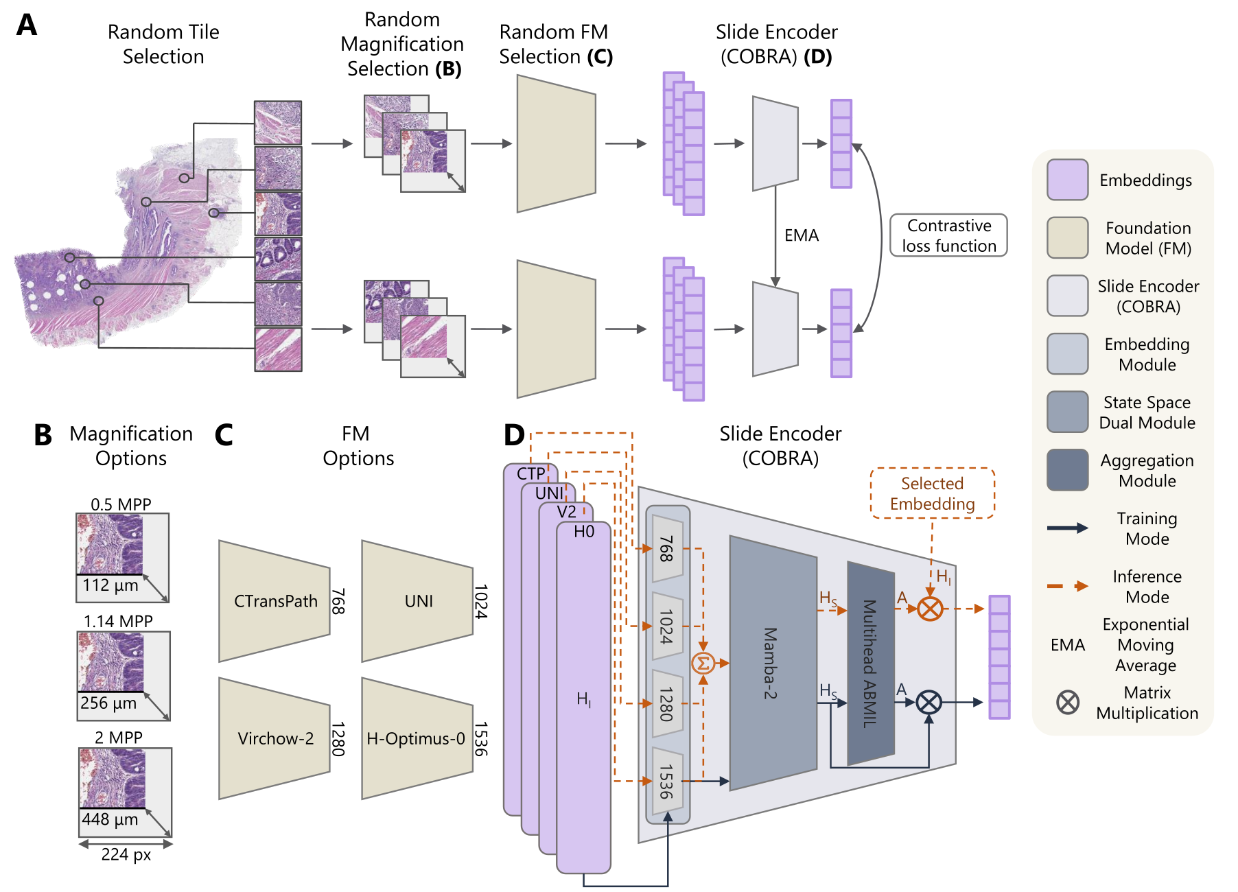
Figure 1: cobra overview for self-supervised slide representation learning (A). A wsi is tessellated into patches at different magnifications (B) and encoded using different foundation models (C) to produce tile embeddings. The magnifications (B) and foundation models (C) serve as feature space augmentations to pretrain the cobra slide encoder (D) using contrastive self-supervised learning.

In recent years, ssl has emerged as a foundational approach in cpath, providing the basis for weakly supervised models to achieve remarkable results in diagnostic, prognostic, and treatment response prediction tasks [3, 40, 26, 36, 18, 25, 4, 9, 38, 43, 23, 10, 46, 31, 27]. By capturing informative, low-dimensional representations from unannotated wsi, ssl has enabled weakly supervised models to use these features for downstream tasks, effectively bridging the gap between high-resolution data and the limited availability of fully annotated datasets. ssl excels in generating low-dimensional feature representations for gigapixel wsi, which can reach dimensions of $\text{150,000}\times\text{150,000}$ pixels, making them challenging to process with vit due to memory constraints. Consequently, most cpath approaches tessellate wsi into smaller patches and extract low-dimensional embeddings for these patches using pretrained histopathology fm [22]. Typically, these patch embeddings are used in weakly-supervised models for downstream classification tasks via mil [7, 15, 34].

In addition to patch-based representations, ssl can also generate slide-level embeddings without any human annotations [19, 20, 45]. Pretrained ssl models can be leveraged to achieve impressive results on downstream tasks with minimal labeled data for task-specific fine-tuning, offering practical advantages like reduced labeling costs, elimination of noisy labels inherent to inter-observer variability, and improved generalizability through label-free representations. Central to ssl is the alignment of multiple representations of wsi or related modalities (e.g., morphological text descriptions) into a shared latent space using contrastive learning or other similarity-based pretraining methods. However, generating effective augmentations to create these representations remains challenging. While image-level augmentations have been widely explored for patch-based learning, they may fail to produce diverse feature augmentations, as many modern FMs are designed to be invariant to these transformations [42, 28]. Other approaches, such as using different stainings (e.g., HE combined with IHC), have shown potential but are limited by the availability of multi-stained tissue samples [17]. Similarly, aligning multiple modalities, such as text or gene expression data, has produced promising results but is constrained by the limited availability of such datasets and requires additional compute to process the different modalities [33, 41, 16].

To address these challenges, we propose a novel ssl method for image-only slide representation learning called cobra. cobra integrates tile embeddings from multiple FMs to generate augmentations directly in feature space, which can then be used to train a slide- or patient-level encoder. By employing Mamba-2 [6] followed by multi-head gated attention [17] and a contrastive loss objective, cobra produces robust slide-level embeddings. Our contributions are summarized as follows:

• We propose an unsupervised single-modality contrastive slide encoder framework (cobra) that avoids the need for stochastic image augmentations as it is trained and deployed on frozen patch embeddings. Extensive evaluations across 15 downstream classification tasks on three tissue types with external validation demonstrate cobra superiority over existing slide encoders.

• Our patient level encoder produces sota unsupervised slide representations with unprecedented data efficiency, outperforming existing approaches with only a fraction of the pretaining data (3048 wsi across four tissue types).

• We show that cobra can turn patch level fm, including ones not encountered during training, into better slide level feature extractors without any additional finetuning, making it particularly valuable as new fm emerge.

• cobra can be deployed across different wsi magnifications, where lower magnifications yield significant gains in computational efficiency with minimal sacrifice of downstream classification performance.

2 Related work

Patch representation learning

Most works applying ssl focus on creating embeddings from image patches. Training a vit with an ssl method like Dino-v2 [29] is now the preferred approach for learning task-agnostic image representations in cpath. sota fm usually combine alignment- and reconstruction-based objectives trained with a student-teacher learning paradigm. These fm are trained on increasingly large datasets and architectures (e.g. vit-Giant [43] or trained on up to 3M wsi [46]). Besides image-only fm, vision-language pathology fm have recently emerged which rely on large-scale paired data [14, 23].

Multiple instance learning

The sota approach for wsi classification is generating tile embeddings using fm and then using these embeddings in a mil approach to train an aggregator model for a specific downstream task. In particular, Attention-based MIL (ABMIL) [15] and many extensions thereof have been proposed [22, 39, 9, 34, 44]. While MIL approaches are prevalent for WSI classification, they are typically supervised and tailored to specific tasks.

Slide representation learning

In contrast to mil, slide representation learning constructs embeddings in an unsupervised manner and is task-agnostic. This next frontier in representation learning of histology images has been proposed in several works. In early work, Chen et al. proposed a hierarchical self-distillation approach for learning unsupervised wsi-level representations [3]. Lazard et al. used augmented patches to create many embeddings of the same input image to enable contrastive learning with slide embeddings [20]. In GigaPath, Xu et al. trained a masked autoencoder on the embeddings of their patch encoder to obtain slide representations [43]. More recent work applied vast amounts of multimodal data to pretrain aggregation models [33, 41, 17]. Differing from previous methodologies, we achieve state-of-the-art wsi-patient-level encoding by performing self-supervised contrastive learning on frozen vision features with a fraction of the data volume. None of the mentioned studies used less than 10K wsi for WSI-level encoder pretraining [3, 20, 17, 41], while PRISM [33] and Gigapath [43] were trained on over 100K WSIs. cobra surpasses the performance of earlier work, even though it is trained on only 3K publicly available WSIs (see Table 1).

Table 1: Slide encoder overview. Abbreviations are as follows: # Ps refers to the number of Parameter and # WSI[K] refers to the number of wsi the slide encoder was pretrained on.

Model	# Ps[M]	# WSI[K]	Patch FM
Gigapath-SE [43]	86	171	Gigapath [43]
CHIEF [41]	1	60	CTransPath [40]
PRISM [33]	513	587	Virchow [38]
MADELEINE [17]	5	69	CONCH [23]
cobra	15	3	CTransPath [40],
			UNI [4],
			Virchow2 [46],
			H-Optimus-0 [31]

3 Method

cobra is an unsupervised slide representation learning framework. Given a set of wsi $\{\mathbf{X}_{i}|\mathbf{X}_{i}\in\mathbb{R}^{d_{x}\times d_{y}\times 3}\}$ belonging to a single patient, it produces a single $d$-dimensional feature vector $\bm{z}\in\mathbb{R}^{d}$ representing that patient. We provide a brief overview of cobra below and in Fig. 1, before going into detail in the following subsections.

cobra operates on preprocessed patch embeddings (Sec. 3.1) from a set of CPath fm. Its architecture consists of a Mamba-2 [6] encoding module, a multi-head attention-based pooling module for learning a patient-level slide embedding (Sec. 3.2) and an embedding module that learns to align multiple fm into the same embedding space. cobra can be deployed in various different modes, which makes it very flexible to adapt to different fm (see Sec. 3.3). We train cobra using a contrastive loss [37] (Sec. 3.4) and evaluate it on a variety of external validation tasks (Sec. 4).

3.1 Preprocessing

Given a histology slide $(\mathbf{X}_{i}\in\mathbb{R}^{d_{x}\times d_{y}\times 3})$, we tessellate the slide into ($224\times 224$) px patches and remove background tiles by employing Canny background detection [30]. Next, we extract patch embeddings with pretrained fm and pool the resulting feature vectors into a slide embedding. We use $fe_{n}$ to refer to the $n\textsuperscript{th}$ fm, $fe_{n}\in\{\text{CTP},\text{UNI},\text{V2},\text{H0}\}$ denoting CTransPath [40], UNI [4], Virchow2 [46], and H-optimus-0 [31], respectively. By integrating fm of different sizes and with different strengths, we aim to capture a diverse set of morphological features and ensure that our slide representations are robust and that cobra is adaptable to other fm. We obtain the patch embeddings $\bm{H}^{fe_{n}}\in\mathbb{R}^{N_{t}\times d_{n}}$ with $N_{t}$ and $d_{n}$ denoting the number of tiles and the embedding dimension $d_{n}\in ds=\{\text{768},\text{1024},\text{1280},\text{1536}\}$.

We extract patch embeddings at 0.5, 1.14 and 2 mpp using 3048 wsi from 2848 patients in tcga BRCA, CRC, LUAD, LUSC and STAD. The use of multiple magnifications acts as a form of data augmentation in feature space, enriching the model’s learning by providing multiscale contextual information. This approach enhances the model’s ability to learn scale-invariant representations and improves its generalization across different tasks.

3.2 Architecture

The slide encoder consists of individual embedding MLPs for the different fm and two Mamba-2 layers [6] followed by multihead gated attention [17, 15]. The embedding module is a layer norm [1] followed by an MLP with one hidden layer and SiLU activation [13]. It projects the different embedding dimensions of the fm to the shared embedding space of the slide encoder. Inspired by MambaMIL [44], we use two Mamba [11] layers to efficiently encode the feature embeddings. We opt for the Mamba-2 ssd modules as they scale substantially better for higher state-space dimensions compared to original Mamba modules [6]. Additional information about the used hyperparamters can be found in Appendix A.

Formally, the architecture may be described as follows:
Let $f_{SE}:\mathbb{R}^{N_{t}\times ds}\to\mathbb{R}^{d}$ denote the slide encoder consisting of three submodules $f_{E}:\mathbb{R}^{N_{t}\times ds}\to\mathbb{R}^{N_{t}\times d}$, $f_{S}:\mathbb{R}^{N_{t}\times d}\to\mathbb{R}^{N_{t}\times d}$ and $f_{A}:\mathbb{R}^{N_{t}\times d}\to\mathbb{R}^{d}$, given by

$$\bm{z}=f_{SE}(\bm{H}^{fe_{n}})=f_{A}(f_{S}(f_{E}(\bm{H}^{fe_{n}}))),~{}\bm{H}^{fe_{n}}\in\mathbb{R}^{N_{t}\times d_{k}},$$ (1)

where $f_{E}$,$f_{S}$,$f_{A}$ denote the embedding module, the state-space dual module and the aggregation module, respectively, and $d_{k}\in ds=\{\text{768},\text{1024},\text{1280},\text{1536}\}$ and $\bm{H}^{fe_{n}}$ refers to the patch embedding of the $n\textsuperscript{th}$ fm. The embedding module $f_{E}$ is defined as follows:

$$\bm{H}_{E}=f_{E}(\bm{H}^{fe_{n}})=\text{Lin}(\text{SiLU}(\text{Lin}(\text{LN}(\bm{H}^{fe_{n}})))),$$ (2)

where Lin denotes a linear layer and LN denotes layer norm. The state-space dual module $f_{S}$ is specified as:

$$\bm{H}_{S}=f_{S}(\bm{H}_{E})=\text{Lin}(\text{SSD}(\text{SSD}(\bm{H}_{E})+\bm{H}_{E})+\bm{H}_{E}).$$ (3)

The aggregation module $f_{A}$ consists of multi-head gated attention [17, 15] to aggregate the input embeddings into a single feature vector via a weighted average. For multi-head gated attention, the encoded embeddings are split into $M$ parts for the $M$ heads: $\bm{H}_{S}=\{\bm{H}_{S}^{m}\}_{m\in\{1,\dots,M\}}$ with $\bm{H}^{m}_{S}\in\mathbb{R}^{N_{t}\times\frac{d}{M}}$. The aggregation module $f_{A}$ is given by

$$\begin{split}\bm{z}=f_{A}(\bm{H}_{S})&=\sum\limits_{k=1}^{N_{t}}a_{k}(\bm{H}_{S,k})\cdot\bm{H}_{S,k};\\ a_{k}(\bm{H}_{S,k})&=\frac{1}{M}\sum\limits_{m=1}^{M}a^{m}_{k}(\bm{H}_{S,k}^{m}),\end{split}$$ (4)

with $\bm{H}_{S,k}\in\mathbb{R}^{d}$ and

$$a_{k}^{m}(\bm{H}_{S,k}^{m})=\hskip 184.9429pt$$

$$\quad\frac{\exp\bigg{(}\bm{w}_{m}^{\top}\Big{(}\tanh\big{(}\bm{V}_{m}(\bm{H}_{S,k}^{m\top})\big{)}\odot\sigma\big{(}\bm{U}_{m}\bm{H}_{S,k}^{m\top}\big{)}\Big{)}\bigg{)}}{\sum\limits_{i}^{N_{t}}\exp\bigg{(}\bm{w}_{m}^{\top}\Big{(}\tanh\big{(}\bm{V}_{m}\bm{H}_{S,i}^{m\top}\big{)}\odot\sigma\big{(}\bm{U}_{m}\bm{H}_{S,i}^{m\top}\big{)}\Big{)}\bigg{)}},$$ (5)

with $\sigma$ denoting the sigmoid function and $\bm{w}\in\mathbb{R}^{p\times 1},\bm{U}\in\mathbb{R}^{p\times d},\bm{V}\in\mathbb{R}^{p\times d}$ as learnable parameters and $p$ being the attention dimension.

3.3 Inference modes

During self-supervised pretraining, the slide encoder learns to map the patch embeddings ($\bm{H}^{fe_{n}}$) of different slides, patches, foundation models and magnifications from the same patient to be close in slide embedding space ($\bm{z}$). For this purpose, encoded embeddings are aggregated to a single feature vector.

Single-fm inference mode

In line with Wang et al. [41], we found it beneficial at inference time to compute the weighted average in Eq. 4 using the original patch embeddings ($\bm{H}^{fe_{n}}$) instead of the encoded embeddings ($\bm{H}_{S}$) to obtain the slide-level representation (see Tab. 6). Importantly, we still use the encoded embeddings to compute the weighting $a_{k}(\bm{H}_{S,k})$ of that average. Specifically, at inference time, Eq. 4 becomes

$$\bm{z}=f_{A_{\text{inf}}}(\bm{H}_{S},\bm{H}^{fe_{n}})=\sum\limits_{k}^{N_{t}}a_{k}(\bm{H}_{S,k})\cdot\bm{H}_{k}^{fe_{n}}.$$ (6)

We refer to this as the single-fm inference mode of cobra and provide an ablation for the choice of Eq. 4 vs. Eq. 6 in Tab. 6.

Combined-fm inference mode

Additionally, one can use feature vectors from all the different foundation models and average the embeddings after the embedding module to extract patient-level features which incorporate the knowledge of the different fm simultaneously with $f_{{SE}_{\text{inf}}}^{\dagger}:\mathbb{R}^{N_{t}\times ds}\times\mathbb{R}^{N_{t}\times d_{k}}\to\mathbb{R}^{d}$ ($d_{k}\in ds$):

$$\begin{split}\bm{z}^{\dagger}&=f_{{SE}_{\text{inf}}}^{\dagger}\big{(}\{\bm{H}^{fe_{n}}\}_{n\in\{1,\dots,N_{FM}\}},\bm{H}^{fe_{l}}\big{)}\\ &=f_{A_{\text{inf}}}\Bigg{(}f_{S}\bigg{(}\frac{\sum^{N_{FM}}_{n}f_{E}^{\dagger}(\bm{H}^{fe_{n}})}{N_{FM}}\bigg{)},\bm{H}^{fe_{l}}\Bigg{)}.\end{split}$$ (7)

Here, $N_{FM}$ denotes the number of foundation models used for pretraining and $\bm{H}^{fe_{l}}$ refers to the patch embeddings that are aggregated during inference.

Unless stated otherwise, we will denote as cobra the combined-fm inference mode version using Virchow2 patch embeddings as input, which is given by

$$\bm{z}^{\dagger}=f_{{SE}_{\text{inf}}}^{\dagger}\big{(}\{\bm{H}^{fe_{n}}\}_{n\in\{1,\dots,N_{FM}\}},\bm{H}^{V2}\big{)}.$$ (8)

3.4 Contrastive loss function

Following He et al. [12], we interpret contrastive learning as training an encoder for a dictionary look-up task:

Consider a set of encoded samples, denoted as $K=\{\bm{k}_{1},\bm{k}_{2},\dots,\bm{k}_{N}\}$, which represent the keys of a dictionary. For a given query $\bm{q}$, there exists exactly one matching key $\bm{k}^{+}\in K$. The contrastive loss is minimized when $\bm{q}$ closely matches $\bm{k}^{+}$ and diverges from all other keys. The InfoNCE [37] loss function is defined as

$$\mathcal{L}_{\mathbf{q}}=-\log\frac{\psi(\mathbf{q},\mathbf{k^{+}})}{\sum\limits_{i=1}^{N}\psi(\mathbf{q},\mathbf{k_{i}})},$$ (9)

where $\bm{q}$ and the corresponding $\bm{k}^{+}$ represent feature vectors produced by a randomly selected pretrained encoder, sampling patches from wsi of the same patient and $N$ is the batch size or the length of the memory queue. The function $\psi$ is defined as follows:

$$\psi(\mathbf{x_{1}},\mathbf{x_{2}})=\exp(\text{sim}(\mathbf{x_{1}},\mathbf{x_{2}})/\tau),$$ (10)

where $\tau$ denotes the temperature parameter and the cosine similarity function is depicted as $\text{sim}(\cdot)$. To avoid feature collapse, the keys and queries should be generated by distinct encoders. Let $\theta_{q}$ denote the parameters of the query encoder with the dense projection head, then the parameters of the key encoder $\theta_{k}$ are updated as follows:

$$\theta_{k}\leftarrow m\theta_{k}+(1-m)\theta_{q},$$ (11)

where $m\in[0,1)$ is the momentum coefficient. With the key encoder as the exponential average of the query encoder, the key representations stay more consistent, which enables a more stabilized training process. We adapted the public MoCo-v3 [5] repository for our experiments to align the embedding space of the slide embeddings generated with tile embeddings from different fm.

Table 2: Comparison of different slide encoder and mean baselines. AUC performance of downstream tasks trained on TCGA and deployed on CPTAC. Overline indicates mean over patch embeddings, ^† indicates that embeddings of all four training FMs were used to generate the weighting vector (Eq. 7). Bold indicates the best performance, and underline indicates the second-best performance. We report the mean score across the five folds in the target columns and the standard deviation as subscript.

AUC[%]

NSCLC

LUAD

BRCA

COAD

Average

Model

ST

STK11

EGFR

ESR1

PGR

ERBB2

PIK3CA

MSI

BRAF

LN

KRAS

Side

PIK3CA

$\overline{\text{Virchow}}$ [38]

$89.7_{1.0}$

$58.6_{8.0}$

$51.0_{5.0}$

$61.1_{5.1}$

$54.8_{3.1}$

$54.5_{5.8}$

$55.5_{7.4}$

$58.6_{4.0}$

$62.7_{2.7}$

$57.0_{5.2}$

$47.8_{9.6}$

$54.1_{1.6}$

$50.2_{3.3}$

$58.1_{5.3}$

$\overline{\text{CTransPath}}$ [40]

$89.0_{1.4}$

$57.7_{5.0}$

$52.5_{3.6}$

$62.8_{1.2}$

$63.4_{1.7}$

$49.3_{1.4}$

$54.9_{1.6}$

$68.1_{7.4}$

$58.8_{5.5}$

$58.7_{4.8}$

$52.5_{9.1}$

$51.2_{7.0}$

$51.7_{4.0}$

$59.3_{4.8}$

$\overline{\text{CONCH}}$ [23]

$96.4_{0.3}$

$69.6_{1.6}$

$57.2_{1.7}$

$78.1_{1.8}$

$75.5_{1.7}$

$64.3_{2.2}$

$57.8_{6.3}$

$71.6_{7.4}$

$59.4_{3.0}$

$\mathbf{61.5}_{5.6}$

$55.3_{6.1}$

$55.6_{3.2}$

$53.3_{9.4}$

$65.8_{4.7}$

$\overline{\text{H-Optimus}}$ [31]

$96.6_{0.6}$

$67.7_{3.8}$

$58.1_{7.6}$

$81.6_{2.1}$

$72.1_{2.8}$

$53.1_{4.3}$

$59.0_{5.1}$

$74.8_{2.9}$

$\underline{84.0}_{0.7}$

$57.9_{7.7}$

$49.6_{5.7}$

$56.9_{8.6}$

$55.5_{4.1}$

$66.7_{5.0}$

$\overline{\text{UNI}}$ [4]

$96.2_{0.8}$

$70.2_{5.6}$

$48.0_{3.6}$

$85.8_{5.0}$

$75.8_{3.3}$

$61.8_{4.5}$

$53.5_{5.1}$

$79.7_{5.1}$

$73.4_{3.1}$

$55.9_{8.4}$

$56.7_{4.5}$

$\mathbf{63.6}_{5.1}$

$51.0_{8.3}$

$67.0_{5.2}$

$\overline{\text{GigaPath}}$ [43]

$96.8_{0.6}$

$63.8_{3.5}$

$47.2_{10.0}$

$84.9_{1.7}$

$74.4_{1.9}$

$64.0_{3.4}$

$57.6_{9.9}$

$\underline{87.5}_{3.8}$

$76.7_{4.5}$

$59.2_{4.7}$

$\mathbf{61.4}_{8.1}$

$\underline{61.6}_{1.7}$

$50.0_{5.3}$

$68.1_{5.4}$

$\overline{\text{Virchow2}}$ [46]

$95.8_{0.5}$

$66.3_{2.8}$

$56.5_{3.6}$

$\underline{88.7}_{0.7}$

$\underline{79.0}_{1.9}$

$\mathbf{73.8}_{3.3}$

$57.3_{6.1}$

$78.4_{17.3}$

$83.0_{2.6}$

$59.2_{3.1}$

$\underline{60.9}_{1.8}$

$59.7_{2.1}$

$50.3_{5.8}$

$\underline{69.9}_{5.8}$

GigaPath-SE [43]

$79.0_{5.3}$

$54.1_{4.1}$

$53.9_{6.6}$

$48.2_{6.3}$

$45.9_{2.3}$

$52.2_{6.1}$

$54.0_{4.1}$

$48.7_{2.8}$

$50.0_{5.1}$

$47.5_{2.1}$

$51.8_{4.4}$

$53.5_{1.0}$

$\mathbf{59.6}_{5.5}$

$53.7_{4.6}$

MADELEINE [17]

$93.7_{0.3}$

$57.1_{14.9}$

$54.5_{8.8}$

$74.8_{2.4}$

$66.6_{10.8}$

$65.0_{1.9}$

$\mathbf{63.6}_{1.4}$

$67.6_{7.9}$

$58.4_{1.9}$

$59.3_{6.6}$

$53.6_{3.3}$

$50.2_{1.0}$

$51.2_{7.7}$

$62.7_{6.8}$

CHIEF [41]

$94.7_{0.6}$

$56.4_{5.9}$

$54.7_{7.3}$

$82.8_{0.6}$

$76.5_{0.3}$

$62.6_{1.7}$

$60.5_{6.7}$

$70.5_{8.8}$

$67.1_{5.1}$

$58.6_{10.4}$

$56.0_{8.7}$

$48.9_{2.3}$

$54.8_{3.2}$

$64.9_{5.8}$

PRISM [33]

$\mathbf{99.1}_{0.1}$

$\underline{70.5}_{3.3}$

$\underline{60.3}_{7.3}$

$\mathbf{91.0}_{0.4}$

$\mathbf{83.2}_{1.6}$

$69.9_{3.5}$

$\underline{61.8}_{7.3}$

$67.5_{9.7}$

$57.2_{1.9}$

$\underline{60.2}_{8.8}$

$57.1_{7.6}$

$49.4_{1.5}$

$53.6_{8.1}$

$67.8_{5.8}$

Cobra

$\underline{98.6}_{0.2}$

$\mathbf{70.7}_{5.5}$

$\mathbf{63.0}_{3.9}$

$87.7_{3.0}$

$78.5_{2.6}$

$\underline{71.6}_{3.0}$

$55.5_{10.4}$

$\mathbf{88.4}_{0.3}$

$\mathbf{86.2}_{2.8}$

$58.1_{6.0}$

$58.1_{6.9}$

$55.3_{5.5}$

$\underline{58.9}_{2.5}$

$\mathbf{71.6}_{4.9}$

4 Experiments & results

4.1 Dataset

TCGA

We collected 3048 WSIs from 2848 patients using the cohorts TCGA [35] Breast Invasive Carcinoma (TCGA-BRCA, 1112 wsi), TCGA Colorectal Carcinoma (TCGA-CRC, 566 wsi), TCGA Lung Adenocarcinoma (TCGA-LUAD, 524 wsi), TCGA Lung Squamous Cell Carcinoma (TCGA-LUSC, 496 wsi), and TCGA Stomach Adenocarcinoma (TCGA-STAD, 350 wsi). See Appendix B for detailed information. These cohorts were used for pretraining cobra and for training the downstream classifiers and linear regression models. We emphasize that neither cobra nor any FMs used in this study were pretrained on datasets included in the evaluation of the downstream tasks, precluding any data leakage.

CPTAC

We collected 1604 WSIs from 444 patients using the cohorts CPTAC [8] Breast Invasive Carcinoma (CPTAC-BRCA, 395 wsi), CPTAC Colon Adenocarcinoma (CPTAC-COAD, 233 wsi), CPTAC Lung Adenocarcinoma (CPTAC-LUAD, 498 wsi), and CPTAC Lung Squamous Cell Carcinoma (CPTAC-LUSC, 478 wsi). These cohorts were exclusively used for external validation.

4.2 Pretraining setup

We trained cobra on patch embeddings derived from slides of 2848 patients, using a batch size of 1024 across four NVIDIA A100 GPUs for 2000 epochs, which took approximately 40 hours. In total, we used 36576 extracted feature embeddings consisting of 3048 wsi for each of the four foundation models and each of the three magnifications included into the pretraining. Additional information about the hyperparameters used for the training of cobra can be found in the Appendix Tab. 5.

Table 3: Ablation over different inference modes. AUC performance of Cobra embeddings compared to mean embeddings of the FMs involved. Overline indicates mean over patch embeddings, ^† indicates that embeddings of all four training FMs were used to generate the weighting vector (Eq. 7). For the other cobra entries, we used the inference mode from (Eq. 6). Bold indicates the best performance, and underline indicates the second-best performance. The abbreviations are as follows: CTP: CTransPath [40], H0: H-Optimus-0 [31], V2: Virchow-2 [46], GP: GigaPath [43]. The different magnifications (5$\times$, 9$\times$, 20$\times$) indicate which magnification of the WSIs was used to extract the embeddings.

AUC[%]

NSCLC

LUAD

BRCA

COAD

Average

Model

ST

STK11

EGFR

ESR1

PGR

ERBB2

PIK3CA

MSI

BRAF

LN

KRAS

Side

PIK3CA

$\overline{\text{CTransPath}}$ [40]

$89.0_{1.4}$

$57.7_{5.0}$

$52.5_{3.6}$

$62.8_{1.2}$

$63.4_{1.7}$

$49.3_{1.4}$

$54.9_{1.6}$

$68.1_{7.4}$

$58.8_{5.5}$

$58.7_{4.8}$

$52.5_{9.1}$

$51.2_{7.0}$

$51.7_{4.0}$

$59.3_{4.8}$

$\overline{\text{H-Optimus}}$ [31]

$96.6_{0.6}$

$67.7_{3.8}$

$58.1_{7.6}$

$81.6_{2.1}$

$72.1_{2.8}$

$53.1_{4.3}$

$59.0_{5.1}$

$74.8_{2.9}$

$84.0_{0.7}$

$57.9_{7.7}$

$49.6_{5.7}$

$56.9_{8.6}$

$55.5_{4.1}$

$66.7_{5.0}$

$\overline{\text{UNI}}$ [4]

$96.2_{0.8}$

$70.2_{5.6}$

$48.0_{3.6}$

$85.8_{5.0}$

$75.8_{3.3}$

$61.8_{4.5}$

$53.5_{5.1}$

$79.7_{5.1}$

$73.4_{3.1}$

$55.9_{8.4}$

$56.7_{4.5}$

$\mathbf{63.6}_{5.1}$

$51.0_{8.3}$

$67.0_{5.2}$

$\overline{\text{GigaPath}}$ [43]

$96.8_{0.6}$

$63.8_{3.5}$

$47.2_{10.0}$

$84.9_{1.7}$

$74.4_{1.9}$

$64.0_{3.4}$

$57.6_{9.9}$

$87.5_{3.8}$

$76.7_{4.5}$

$59.2_{4.7}$

$\underline{61.4}_{8.1}$

$\underline{61.6}_{1.7}$

$50.0_{5.3}$

$68.1_{5.4}$

$\overline{\text{Virchow2}}$ [46]

$95.8_{0.5}$

$66.3_{2.8}$

$56.5_{3.6}$

$88.7_{0.7}$

$\underline{79.0}_{1.9}$

$\mathbf{73.8}_{3.3}$

$57.3_{6.1}$

$78.4_{17.3}$

$83.0_{2.6}$

$59.2_{3.1}$

$60.9_{1.8}$

$59.7_{2.1}$

$50.3_{5.8}$

$69.9_{5.8}$

Cobra-CTP

$96.5_{0.6}$

$56.1_{8.3}$

$58.8_{2.9}$

$76.3_{0.9}$

$69.2_{1.5}$

$60.3_{2.3}$

$60.4_{3.2}$

$72.7_{9.8}$

$74.6_{5.0}$

$60.7_{3.6}$

$57.8_{4.5}$

$52.2_{8.0}$

$52.7_{2.2}$

$65.3_{5.0}$

Cobra-UNI

$99.1_{0.1}$

$\mathbf{72.0}_{4.3}$

$55.4_{7.2}$

$87.9_{1.7}$

$78.9_{1.0}$

$64.6_{3.7}$

$62.0_{3.7}$

$85.5_{2.3}$

$76.9_{4.7}$

$53.5_{7.5}$

$57.2_{7.6}$

$58.4_{6.6}$

$53.3_{4.3}$

$69.6_{4.8}$

Cobra-H0

$\mathbf{99.4}_{0.2}$

$66.5_{7.7}$

$58.6_{16.1}$

$88.8_{1.1}$

$72.6_{4.0}$

$61.0_{3.1}$

$58.3_{2.9}$

$86.1_{2.2}$

$\mathbf{88.0}_{2.1}$

$60.2_{2.4}$

$54.6_{6.1}$

$58.5_{5.7}$

$\mathbf{61.2}_{2.9}$

$70.3_{5.9}$

Cobra-V2

$98.4_{0.2}$

$68.0_{5.1}$

$62.2_{3.8}$

$87.4_{3.4}$

$77.2_{1.1}$

$70.0_{2.8}$

$61.5_{5.1}$

$85.7_{5.2}$

$86.9_{1.7}$

$\underline{60.9}_{4.4}$

$58.7_{5.5}$

$55.2_{4.9}$

$56.7_{0.9}$

$\underline{71.4}_{3.8}$

Cobra†-CTP

$96.4_{0.6}$

$59.1_{7.3}$

$54.6_{13.2}$

$75.7_{0.9}$

$65.2_{6.2}$

$56.6_{3.8}$

$57.7_{1.8}$

$78.5_{5.1}$

$72.2_{5.4}$

$\mathbf{61.5}_{7.1}$

$56.0_{5.1}$

$53.6_{5.0}$

$51.8_{5.9}$

$64.5_{6.1}$

Cobra†-UNI

$\underline{99.3}_{0.1}$

$70.3_{4.8}$

$59.2_{4.3}$

$\underline{89.0}_{1.5}$

$77.6_{1.8}$

$58.7_{3.2}$

$62.1_{4.8}$

$76.7_{10.5}$

$79.1_{3.4}$

$52.9_{11.0}$

$60.5_{4.4}$

$60.6_{2.1}$

$52.3_{3.7}$

$69.1_{5.3}$

Cobra†-H0

$\underline{99.3}_{0.2}$

$64.8_{8.8}$

$\mathbf{65.4}_{7.6}$

$88.0_{1.3}$

$74.6_{3.6}$

$58.7_{4.6}$

$59.8_{2.5}$

$83.5_{3.0}$

$\underline{87.7}_{1.9}$

$49.6_{4.6}$

$57.7_{7.4}$

$55.7_{6.1}$

$57.8_{1.4}$

$69.4_{4.8}$

Cobra†-V2-5$\times$

$99.1_{0.1}$

$64.8_{11.5}$

$61.8_{3.9}$

$88.0_{1.0}$

$\mathbf{79.7}_{1.1}$

$65.6_{2.1}$

$62.1_{5.8}$

$87.1_{2.5}$

$84.1_{2.8}$

$57.4_{6.8}$

$\mathbf{67.7}_{2.2}$

$51.6_{3.1}$

$50.9_{8.5}$

$70.8_{5.1}$

Cobra†-V2-9$\times$

$99.0_{0.2}$

$70.1_{4.5}$

$61.9_{4.3}$

$\mathbf{89.7}_{1.0}$

$78.9_{1.7}$

$68.8_{2.7}$

$\mathbf{64.7}_{3.1}$

$\underline{89.1}_{1.9}$

$83.6_{1.3}$

$53.3_{3.4}$

$56.7_{12.2}$

$57.1_{2.8}$

$50.1_{4.7}$

$71.0_{4.4}$

Cobra†-V2-20$\times$

$98.6_{0.2}$

$\underline{70.7}_{5.5}$

$63.0_{3.9}$

$87.7_{3.0}$

$78.5_{2.6}$

$\underline{71.6}_{3.0}$

$55.5_{10.4}$

$88.4_{0.3}$

$86.2_{2.8}$

$58.1_{6.0}$

$58.1_{6.9}$

$55.3_{5.5}$

$\underline{58.9}_{2.5}$

$\mathbf{71.6}_{4.9}$

Cobra†-GP

$99.0_{0.3}$

$64.3_{6.1}$

$\underline{64.5}_{5.2}$

$87.2_{0.7}$

$75.9_{1.9}$

$64.2_{2.9}$

$\underline{63.2}_{4.5}$

$\mathbf{90.4}_{1.5}$

$82.3_{3.6}$

$58.7_{6.9}$

$54.8_{8.9}$

$59.2_{2.8}$

$54.3_{4.0}$

$70.6_{4.5}$

Table 4: Evaluation of the magnification augmentation during pretraining AUC performance of downstream tasks trained on TCGA and deployed on CPTAC ^† indicates that embeddings of all four training FMs were used to generate the weighting vector (Eq. 7), ^∗ indicates that cobra was only trained on 0.5 MPP. Bold indicates the best performance, and underline indicates the second-best performance.

	AUC[%]	NSCLC	LUAD		BRCA				COAD						Average
	Model	ST	STK11	EGFR	ESR1	PGR	ERBB2	PIK3CA	MSI	BRAF	LN	KRAS	Side	PIK3CA
5$\times$	Cobra∗-H0	$90.5_{1.0}$	$54.0_{7.4}$	$57.9_{4.5}$	$77.6_{2.0}$	$69.7_{2.3}$	$54.5_{3.2}$	$62.8_{3.6}$	$80.0_{4.5}$	$70.8_{3.3}$	$61.2_{4.2}$	$55.7_{6.3}$	$55.3_{3.6}$	$52.7_{7.5}$	$64.8_{4.5}$
	Cobra∗-CTP	$89.1_{0.8}$	$65.0_{2.4}$	$60.2_{3.6}$	$81.3_{1.3}$	$71.2_{9.8}$	$59.0_{4.5}$	$62.8_{5.8}$	$69.6_{13.3}$	$69.7_{3.7}$	$\underline{61.5}_{6.5}$	$56.4_{9.0}$	$51.6_{1.7}$	$51.2_{4.3}$	$65.3_{6.2}$
	Cobra†-CTP	$96.6_{0.3}$	$62.9_{7.2}$	$58.8_{4.6}$	$81.9_{0.8}$	$74.4_{1.4}$	$64.0_{3.1}$	$\mathbf{65.2}_{2.3}$	$77.4_{4.2}$	$70.3_{4.9}$	$57.9_{9.6}$	$53.3_{8.4}$	$46.2_{2.2}$	$48.4_{4.1}$	$65.9_{4.9}$
	Cobra†-H0	$97.5_{0.6}$	$60.5_{4.6}$	$59.7_{2.8}$	$80.0_{2.5}$	$70.9_{0.8}$	$55.1_{2.4}$	$64.4_{1.5}$	$78.2_{4.1}$	$71.2_{3.1}$	$60.3_{5.1}$	$58.3_{6.2}$	$51.7_{3.9}$	$54.0_{4.9}$	$66.3_{3.7}$
	Cobra†-UNI	$97.7_{0.4}$	$66.8_{4.4}$	$63.3_{2.2}$	$81.9_{1.8}$	$72.7_{1.2}$	$55.6_{2.0}$	$64.9_{5.1}$	$76.9_{2.0}$	$71.4_{2.1}$	$56.2_{11.2}$	$53.0_{4.9}$	$52.5_{4.6}$	$53.5_{9.3}$	$66.6_{5.0}$
	Cobra∗-UNI	$91.6_{1.0}$	$63.8_{5.1}$	$64.2_{4.4}$	$81.5_{2.0}$	$73.2_{2.1}$	$58.5_{2.4}$	$59.1_{12.1}$	$78.5_{4.0}$	$71.1_{3.6}$	$59.0_{2.4}$	$54.4_{6.1}$	$54.8_{3.9}$	$\mathbf{60.4}_{7.8}$	$66.9_{5.2}$
	Cobra†-V2	$99.1_{0.1}$	$64.8_{11.5}$	$61.8_{3.9}$	$88.0_{1.0}$	$\underline{79.7}_{1.1}$	$65.6_{2.1}$	$62.1_{5.8}$	$87.1_{2.5}$	$84.1_{2.8}$	$57.4_{6.8}$	$\mathbf{67.7}_{2.2}$	$51.6_{3.1}$	$50.9_{8.5}$	$70.8_{5.1}$
	Cobra∗-V2	$97.2_{0.4}$	$66.9_{5.5}$	$57.3_{4.9}$	$\mathbf{90.6}_{2.3}$	$\mathbf{80.3}_{1.9}$	$\underline{72.0}_{2.4}$	$61.8_{3.2}$	$87.9_{1.2}$	$81.3_{1.6}$	$60.2_{10.0}$	$63.7_{2.0}$	$57.2_{0.4}$	$51.4_{11.6}$	$\underline{71.4}_{5.0}$
9$\times$	Cobra∗-CTP	$93.8_{0.9}$	$62.1_{8.2}$	$64.9_{3.7}$	$78.7_{1.3}$	$72.0_{0.6}$	$50.7_{7.8}$	$53.3_{8.0}$	$65.5_{11.0}$	$67.7_{2.3}$	$56.1_{5.9}$	$51.7_{5.8}$	$52.3_{4.7}$	$55.0_{6.9}$	$63.4_{6.0}$
	Cobra∗-H0	$97.8_{0.4}$	$62.5_{5.0}$	$64.4_{3.5}$	$83.4_{2.5}$	$73.0_{3.7}$	$58.8_{8.7}$	$59.5_{3.5}$	$75.1_{3.6}$	$67.0_{10.2}$	$60.4_{6.4}$	$57.3_{10.7}$	$58.0_{4.5}$	$51.2_{9.4}$	$66.8_{6.4}$
	Cobra†-CTP	$96.5_{0.3}$	$65.5_{3.0}$	$63.9_{2.5}$	$80.6_{0.6}$	$73.7_{1.1}$	$64.6_{2.0}$	$62.0_{0.9}$	$79.9_{2.8}$	$75.5_{3.6}$	$\mathbf{63.6}_{5.3}$	$54.5_{6.4}$	$46.4_{3.3}$	$48.9_{5.7}$	$67.4_{3.5}$
	Cobra∗-UNI	$97.8_{0.6}$	$65.3_{5.1}$	$\underline{65.6}_{3.6}$	$86.0_{0.8}$	$76.0_{3.5}$	$58.4_{6.1}$	$62.8_{5.2}$	$70.5_{14.4}$	$71.6_{1.9}$	$56.6_{4.0}$	$\underline{66.6}_{2.4}$	$58.8_{2.3}$	$55.3_{6.0}$	$68.6_{5.5}$
	Cobra∗-V2	$97.6_{0.5}$	$61.8_{11.9}$	$57.1_{8.1}$	$88.4_{1.0}$	$78.2_{1.5}$	$67.8_{6.6}$	$57.5_{5.0}$	$82.7_{2.8}$	$73.4_{2.3}$	$50.3_{6.8}$	$64.7_{1.7}$	$57.1_{1.8}$	$56.5_{11.1}$	$68.7_{6.0}$
	Cobra†-UNI	$99.1_{0.2}$	$63.3_{5.7}$	$\mathbf{68.5}_{3.3}$	$86.7_{0.8}$	$76.2_{2.0}$	$60.1_{3.8}$	$\underline{65.0}_{4.2}$	$81.3_{1.7}$	$78.3_{4.6}$	$58.3_{7.5}$	$60.3_{5.3}$	$59.3_{2.0}$	$52.6_{4.3}$	$69.9_{4.0}$
	Cobra†-H0	$\underline{\mathbf{99.3}}_{0.3}$	$66.7_{5.1}$	$65.5_{3.0}$	$85.2_{0.7}$	$76.4_{1.4}$	$64.3_{3.7}$	$62.7_{3.5}$	$85.1_{2.4}$	$82.8_{4.6}$	$57.7_{10.8}$	$59.1_{8.4}$	$58.8_{5.1}$	$53.7_{3.1}$	$70.6_{4.9}$
	Cobra†-V2	$99.0_{0.2}$	$70.1_{4.5}$	$61.9_{4.3}$	$\underline{89.7}_{1.0}$	$78.9_{1.7}$	$68.8_{2.7}$	$64.7_{3.1}$	$\mathbf{89.1}_{1.9}$	$83.6_{1.3}$	$53.3_{3.4}$	$56.7_{12.2}$	$57.1_{2.8}$	$50.1_{4.7}$	$71.0_{4.4}$
20$\times$	Cobra∗-CTP	$95.2_{1.0}$	$54.0_{11.2}$	$61.7_{2.5}$	$73.4_{2.2}$	$67.1_{1.7}$	$59.2_{3.1}$	$53.0_{2.1}$	$76.6_{5.8}$	$70.3_{3.5}$	$54.8_{7.3}$	$53.6_{10.9}$	$56.7_{3.9}$	$56.3_{5.8}$	$64.0_{5.7}$
	Cobra†-CTP	$96.4_{0.6}$	$59.1_{7.3}$	$54.6_{13.2}$	$75.7_{0.9}$	$65.2_{6.2}$	$56.6_{3.8}$	$57.7_{1.8}$	$78.5_{5.1}$	$72.2_{5.4}$	$\underline{61.5}_{7.1}$	$56.0_{5.1}$	$53.6_{5.0}$	$51.8_{5.9}$	$64.5_{6.1}$
	Cobra∗-UNI	$98.3_{0.3}$	$\mathbf{73.2}_{8.9}$	$58.6_{5.2}$	$86.9_{2.5}$	$72.9_{3.0}$	$62.5_{2.9}$	$57.9_{5.4}$	$82.6_{3.0}$	$74.3_{1.5}$	$52.9_{6.2}$	$59.3_{11.3}$	$\underline{64.4}_{3.2}$	$44.0_{9.5}$	$68.3_{5.8}$
	Cobra†-UNI	$\underline{\mathbf{99.3}}_{0.1}$	$70.3_{4.8}$	$59.2_{4.3}$	$89.0_{1.5}$	$77.6_{1.8}$	$58.7_{3.2}$	$62.1_{4.8}$	$76.7_{10.5}$	$79.1_{3.4}$	$52.9_{11.0}$	$60.5_{4.4}$	$60.6_{2.1}$	$52.3_{3.7}$	$69.1_{5.3}$
	Cobra†-H0	$\underline{\mathbf{99.3}}_{0.2}$	$64.8_{8.8}$	$65.4_{7.6}$	$88.0_{1.3}$	$74.6_{3.6}$	$58.7_{4.6}$	$59.8_{2.5}$	$83.5_{3.0}$	$\mathbf{87.7}_{1.9}$	$49.6_{4.6}$	$57.7_{7.4}$	$55.7_{6.1}$	$57.8_{1.4}$	$69.4_{4.8}$
	Cobra∗-H0	$98.8_{0.1}$	$67.5_{7.9}$	$65.4_{6.4}$	$86.2_{1.9}$	$75.6_{1.8}$	$64.6_{3.6}$	$49.5_{3.5}$	$81.0_{3.6}$	$80.4_{2.3}$	$56.9_{2.2}$	$55.6_{5.7}$	$\mathbf{65.0}_{6.3}$	$56.3_{8.8}$	$69.4_{4.9}$
	Cobra∗-V2	$97.0_{0.2}$	$\underline{71.4}_{2.8}$	$61.3_{3.6}$	$88.1_{1.8}$	$78.1_{2.4}$	$\mathbf{72.7}_{3.3}$	$56.3_{4.0}$	$84.1_{2.6}$	$82.7_{1.8}$	$56.0_{4.2}$	$60.4_{5.6}$	$55.5_{8.9}$	$51.1_{8.1}$	$70.4_{4.5}$
	Cobra†-V2	$98.6_{0.2}$	$70.7_{5.5}$	$63.0_{3.9}$	$87.7_{3.0}$	$78.5_{2.6}$	$71.6_{3.0}$	$55.5_{10.4}$	$\underline{88.4}_{0.3}$	$\underline{86.2}_{2.8}$	$58.1_{6.0}$	$58.1_{6.9}$	$55.3_{5.5}$	$\underline{58.9}_{2.5}$	$\mathbf{71.6}_{4.9}$

4.3 Tasks

cpath is used for different task categories. One important such category is biomarker prediction. Here, we focused on STK11, EGFR, KRAS and TP53 mutation prediction in LUAD, ESR1, PGR and ERBB2 expression, and PIK3CA mutation prediction in BRCA, and MSI status, BRAF, KRAS, PIK3CA mutation prediction in COAD. We also included classification of phenotypic subtypes, Non-Small Cell Lung Cancer (NSCLC) Subtyping and Sidedness prediction of COAD. Finally, we added N-Status prediction in COAD, a task that goes beyond the tissue itself and tries to classify whether the tumor has infiltrated lymph nodes, thereby influencing prognostication. KRAS and TP53 in LUAD showed no predictive signal across all models. Therefore, these tasks were excluded from the main findings but are provided in Tab. 6 for completeness alongside the results on other evaluation metrics. We report auroc results in the main text, additional metrics like F1 score, auprc and the balanced accuracy for all experiments can be found in Appendix C. Unless indicated otherwise, all results are reported for 0.5 mpp (20$\times$ wsi magnification). Overall, we did our evaluation experiments for three different wsi magnifications: 0.5 mpp (20$\times$), 1.14 mpp (9$\times$) and 2 mpp (5$\times$). Additional information about the downstream experiments can be found in Sec. A.1.

4.4 Evaluation of patient embeddings

MLP downstream classification

We evaluate cobra patient-level slide embeddings following standard practice in cpath using 5-fold cross-validation on the tcga training cohort followed by deploying all five classifiers on the full external validation set CPTAC. The classifier is a simple MLP. Generating a slide embedding and then training a small MLP is much more efficient than current mil approaches using tile embeddings. We compare cobra to all mean patch embeddings of fm used in this study and to the slide encoders MADELEINE [17], PRISM [33], GigaPath [43] and CHIEF [41] (see Tab. 2). All slide encoders except GigaPath and MADELEINE manage to outperform the mean embeddings of the patch embeddings of the fm they are based upon, however, cobra is the only model that manages to reach a higher macro-AUC than Virchow2 mean patch embeddings. Nevertheless, it should be noted that MADELEINE was trained only on BRCA and Kidney slides where it improves over CONCH. However, cobra also substantially outperforms MADELEINE on the BRCA tasks on all targets but PIK3CA (ESR1: +12.9%, PGR +11.9%, ERBB2 +6.6%, PIK3CA -8.1% AUC). Overall, cobra improves over PRISM by +3.8% average auroc and over the mean of the patch embeddings of Virchow2 by +1.7%. Especially on the COAD downstream tasks, MSI and BRAF, cobra achieves substantial performance increases over the other slide encoders of at least +17.9% average AUC and +19.1% average AUC, respectively.

Linear probing few-shot classification

We also evaluate cobra in a few-shot setting across 10 runs for high-performance tasks, where the mean patch embeddings of at least one fm scores an average macro-AUC of $>$ 0.7 across the five folds of the full classification and where the tcga cohorts contain at least 50 cases per class. These tasks are NSCLC Subtyping, ESR1, PGR and ERBB2 expression prediction in BRCA, and BRAF mutation and MSI status in COAD (see Fig. 2).

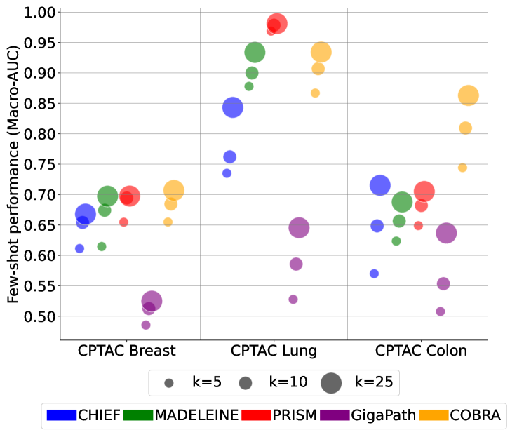
Figure 2: Few shot linear probing classification. Linear probing macro-AUC performance comparison for $k$ samples per class.

Even though cobra was only trained on very few samples and with only one modality, we observe that it is still robust enough to achieve high few-shot performance compared to the other slide encoders. On the BRCA tasks, it slightly outperforms the competition, while it substantially exceeds the results of the other models on the COAD tasks. We provide further results and information about the few shot experiments in Sec. C.2.

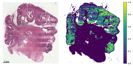
Figure 3: cobra Unsupervised Heatmap. Visualization of the weighting scores for the tiles of a WSI generated by Cobra for Patient-ID TCGA-CA-6716 from TCGA-CRC.

4.5 Inference ablations

Foundation models

As cobra is FM-agnostic, it can be used to enhance small, inferior tile level fm like CTransPath to achieve performances comparable to large sota tile level fm like H-optimus-0 and UNI (-1.4%, -1.7% average AUC) while cobra-CTP also improves over all slide encoders but PRISM (see Tabs. 3 and 2). This substantially improves efficiency, as CTransPath has approximately 30M parameters, compared to over 600M in Virchow2 and more than 1B in H-optimus-0.

Magnifications

Another way to achieve efficiency improvements is reducing the magnification of the wsi for the patch embeddings, which in turn significantly reduces the number of tiles that need to be extracted and embedded. Notably, this change does not result in a significant drop in performance as cobra^†-V2-5$\times$ and cobra^†-V2-9$\times$ achieve performance gains over PRISM of +3% and +3.2% average AUC, respectively (see Tabs. 3 and 2), which we attribute to our multiscale alignment during pretraining.

Combined inference and unseen FMs

In a combined inference mode (indicated by ^† in Tab. 3), where embeddings from all pretrained fm are used, performance is slightly better for larger models like H-optimus-0 and Virchow2, though it does not notably improve the downstream classification performance of UNI or CTransPath. Overall, the performance is comparable to the single-fm mode. Additionally, cobra remains useful for future fm as it can aggregate embeddings from unseen fm and improve their performance over the mean baseline. We show evidence for that by deploying cobra on GigaPath patch embeddings, which improves over PRISM on average by +2.8% AUC (Tabs. 3 and 2).

4.6 Pretraining ablation

Single-magnification architecture

We analyze single-magnification performance by training on only 0.5 mpp embeddings and find that using all three magnifications results in an average AUC improvement of +1.26% AUC across models. For specific scenarios, such as 9$\times$ magnifications in CTransPath and H-optimus-0, the improvement is particularly notable, with AUC increases of +4% and +3.8% AUC, respectively (Tab. 4). Additionally, the three-magnification setup yields substantial gains in NSCLC subtyping at 5$\times$ magnification, with improvements of +6.1% AUC for UNI, +7.5% for CTransPath, +7% for H-optimus-0, and +1.9% for Virchow2. These results indicate that using multiple magnifications can enhance performance in certain cases and does not negatively impact model performance.

4.7 Interpretability

cobra enables unsupervised interpretability as it is an aggregation method of patch embeddings that calculates a weighted average by assigning each tile a softmaxed value, which can be interpreted as an attention value. By visualizing these weightings for wsi, we observe that the model shows high attention values for the tumor regions in the slide (see Fig. 3). It is worth mentioning that for these heatmaps, no GradCam [32] is required, and they are generated only based on patch embeddings, so each tile only receives one value instead of pixel-level attention that can be achieved with other methods. However, this extremely simple approach is sufficient to identify the important tumor regions in detail without any supervision like targeted segmentation training. More examples and detailed explanations can be found in Appendix D.

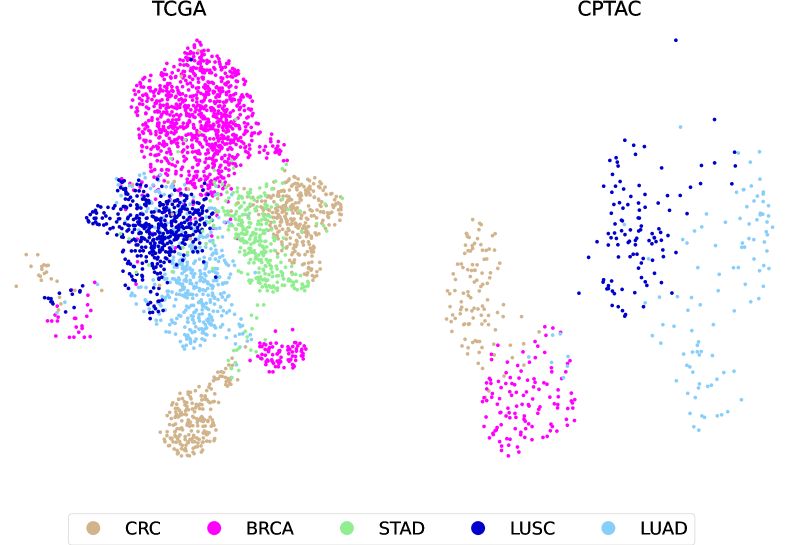
Figure 4: UMAP visualization of cobra’s patient-level slide embeddings for TCGA and CPTAC datasets at $0.5~{}$mpp. Each color represents a different tissue type, with five tissue types in total.

Furthermore, we visualized cobra’s embedding space using umap [24] plots of cobra’s patient-level slide embeddings extracted at $0.5~{}$mpp for TCGA and CPTAC (see Fig. 4). We observe decent separation between the different tissue types involved in this study, indicating that cobra learned meaningful representations that can distinguish between tissue types without supervision.

5 Conclusion

In this paper, we introduced cobra, a novel FM- and task-agnostic approach for slide representation learning. Trained on only 3048 wsi from tcga, cobra achieves sota performance, even surpassing multimodal slide encoders. This is particularly valuable for medical imaging, where acquiring large annotated datasets is challenging due to privacy concerns and annotation costs. While additional data might enhance performance, our results indicate that cobra is highly effective even in low-data regimes. These results highlight the potential of SSL in leveraging the strengths of histopathology FMs. Future work includes exploring SSL objectives that extend beyond contrastive approaches, as well as incorporating more cancer types, pretraining data and a larger variety of FMs into cobra.

Appendix

Appendix A Implementation details

FM pretraining

The detailed pretraining settings for cobra can be found in Tab. 5. We used 25% dropout in all MLPs.

Hyperparameter	Value
Heads	8
Number of Mamba-2 layers	2
Embedding dimension	768
Input dimensions	768, 1024, 1280, 1536
Dropout	0.25
Attention hidden dimension	96
Teacher momentum	0.99
Contrastive loss temperature	0.2
Optimizer	AdamW [21]
Learning rate	5e-4
Warmup epochs	50
Weight decay	0.1
Epochs	2000
Batch size	1024
Features per patient	768

Table 5: Hyperparameters for cobra pretraining

A.1 Additional information on evaluation

A.1.1 MLP downstream classification

An MLP classifier is implemented using a two-layer architecture, with an input layer of 768 dimensions and a hidden layer of 256 dimensions. The hidden layer employs SiLU activation, followed by a dropout layer for regularization. The output layer consists of a fully connected layer with the appropriate number of output classes. Cross-entropy loss with class weighting is applied to handle class imbalance. The classifier is trained using the AdamW optimizer with a learning rate of 0.0001 and weight decay of 0.01, employing a one-cycle policy for 32 epochs. Training is conducted in a 5-fold cross-validation setup, with early stopping and best model checkpoints monitored by validation loss.

A.1.2 Linear probing

Linear probing is implemented using a logistic regression objective based on sklearn. We use the default sklearn L2 regularization (set to 1.0) with an lbfgs solver. We set the maximum iterations to 10,000 and apply balanced class weights. Training is conducted in a stratified sampling setting with 10 random runs, using 5, 10, and 25 cases per class in each run.

Appendix B Data

Overall, our study comprises a total of 4,652 WSIs from 3,292 patients, including the organs lung, stomach, breast and colon. We use 3,048 WSIs for pretraining cobra and training the classifiers, and 1604 WSIs for external validation. The slides for TCGA are available at https://portal.gdc.cancer.gov/. The slides for CPTAC are available at https://proteomics.cancer.gov/data-portal. The molecular data for TCGA and CPTAC are available at https://www.cbioportal.org/[2].

TCGA BRCA (training)

We collected N=1,041 primary cases from the TCGA Breast Invasive Carcinoma (BRCA) cohort. For each case, we downloaded the corresponding molecular status: ER (N=1041; 770 positive, 271 negative), PR (N=1041; 704 positive, 337 negative), HER2 (N=1041; 125 positive, 916 negative), and PIK3CA driver mutation (N=1023; 687 WT, 336 MUT).

TCGA CRC (training)

We collected N=558 primary cases from the TCGA Colorectal Carcinoma (CRC) cohort. For each case, we downloaded the corresponding molecular status: MSI status (N=429; 368 MSS, 61 MSI), Lymph Node status (N=556; 318 N0, 238 N+), CRC sidedness (N=398; 230 left, 168 right), BRAF (N=501; 450 WT, 51 MUT), KRAS (N=501; 296 WT, 205 MUT), and PIK3CA driver mutation (N=501; 377 WT, 124 MUT).

TCGA LUAD (training)

We collected N=461 primary cases from the TCGA Lung Adenocarcinoma (LUAD) cohort. For each case, we downloaded the corresponding molecular status: STK11 (N=461; 394 WT, 67 MUT), EGFR (N=461; 411 WT, 50 MUT), KRAS (N=461; 317 WT, 144 MUT), and TP53 driver mutation (N=461; 239 MUT, 222 WT).

TCGA NSCLC (training)

We collected N=462 primary cases from the TCGA Lung Squamous Cell Carcinoma (LUSC) cohort and the aforementioned N=461 primary cases from the TCGA LUAD cohort.

TCGA STAD (training)

We collected N=326 primary cases from the TCGA Stomach Adenocarcinoma (STAD) cohort. They were only used for the training of cobra.

CPTAC BRCA (testing)

We collected N=120 primary cases from the CPTAC Breast Invasive Carcinoma (BRCA) cohort. For each case, we downloaded the corresponding molecular status: ER (N=120; 79 positive, 41 negative), PR (N=120; 70 positive, 50 negative), HER2 (N=120; 14 positive, 106 negative), and PIK3CA driver mutation (N=120; 82 WT, 38 MUT).

CPTAC COAD (testing)

We collected N=110 primary cases from the CPTAC Colon Adenocarcinoma (COAD) cohort. For each case, we downloaded the corresponding molecular status: MSI status (N=105; 81 MSS, 24 MSI), Lymph Node status (N=110; 56 N0, 54 N+), CRC sidedness (N=108; 51 left, 57 right), BRAF (N=106; 91 WT, 15 MUT), KRAS (N=106; 71 WT, 35 MUT), and PIK3CA driver mutation (N=106; 87 WT, 19 MUT).

CPTAC LUAD (testing)

We collected N=106 primary cases from the CPTAC Lung Adenocarcinoma (LUAD) cohort. For each case, we downloaded the corresponding molecular status: STK11 (N=106; 88 WT, 18 MUT), EGFR (N=106; 72 WT, 34 MUT), KRAS (N=106; 74 WT, 32 MUT), and TP53 driver mutation (N=106; 55 MUT, 51 WT).

CPTAC LUSC (testing)

We collected N=108 primary cases from the CPTAC Lung Squamous Cell Carcinoma (LUSC) cohort and the aforementioned N=106 primary cases from the CPTAC LUAD cohort.

Appendix C Results

C.1 Full Classification

Table 6: Classification performance comparison. AUC performance of models trained on TCGA deployed on CPTAC datasets. Overline indicates mean over patch embeddings, ^† indicates that embeddings of all four training FMs were used to generate the weighting vector (Eq. 7). For the other cobra entries, we used the inference mode from (Eq. 6). Bold indicates the best performance, and underline indicates the second-best performance.The abbreviations are as follows: CTP: CTransPath [40], H0: H-Optimus-0 [31], V2: Virchow-2 [46], GP: GigaPath [43].

AUC-20$\times$[%]	NSCLC	LUAD				BRCA				COAD						Average
Model	ST	STK11	EGFR	TP53	KRAS	ESR1	PGR	ERBB2	PIK3CA	MSI	BRAF	LN	KRAS	Side	PIK3CA
$\overline{\text{Virchow}}$ [38]	$89.7_{1.0}$	$58.6_{8.0}$	$51.0_{5.0}$	$46.2_{4.4}$	$47.2_{6.1}$	$61.1_{5.1}$	$54.8_{3.1}$	$54.5_{5.8}$	$55.5_{7.4}$	$58.6_{4.0}$	$62.7_{2.7}$	$57.0_{5.2}$	$47.8_{9.6}$	$54.1_{1.6}$	$50.2_{3.3}$	$56.6_{5.3}$
$\overline{\text{CTransPath}}$ [40]	$89.0_{1.4}$	$57.7_{5.0}$	$52.5_{3.6}$	$45.1_{12.1}$	$47.9_{1.3}$	$62.8_{1.2}$	$63.4_{1.7}$	$49.3_{1.4}$	$54.9_{1.6}$	$68.1_{7.4}$	$58.8_{5.5}$	$58.7_{4.8}$	$52.5_{9.1}$	$51.2_{7.0}$	$51.7_{4.0}$	$57.6_{5.5}$
$\overline{\text{CONCH}}$ [23]	$96.4_{0.3}$	$69.6_{1.6}$	$57.2_{1.7}$	$45.6_{15.1}$	$51.2_{4.7}$	$78.1_{1.8}$	$75.5_{1.7}$	$64.3_{2.2}$	$57.8_{6.3}$	$71.6_{7.4}$	$59.4_{3.0}$	$\underline{\mathbf{61.5}}_{5.6}$	$55.3_{6.1}$	$55.6_{3.2}$	$53.3_{9.4}$	$63.5_{6.0}$
$\overline{\text{H-Optimus}}$ [31]	$96.6_{0.6}$	$67.7_{3.8}$	$58.1_{7.6}$	$50.6_{3.8}$	$47.6_{5.5}$	$81.6_{2.1}$	$72.1_{2.8}$	$53.1_{4.3}$	$59.0_{5.1}$	$74.8_{2.9}$	$84.0_{0.7}$	$57.9_{7.7}$	$49.6_{5.7}$	$56.9_{8.6}$	$55.5_{4.1}$	$64.3_{4.9}$
$\overline{\text{UNI}}$ [4]	$96.2_{0.8}$	$70.2_{5.6}$	$48.0_{3.6}$	$\underline{51.2}_{5.3}$	$48.4_{7.9}$	$85.8_{5.0}$	$75.8_{3.3}$	$61.8_{4.5}$	$53.5_{5.1}$	$79.7_{5.1}$	$73.4_{3.1}$	$55.9_{8.4}$	$56.7_{4.5}$	$\mathbf{63.6}_{5.1}$	$51.0_{8.3}$	$64.7_{5.4}$
$\overline{\text{GigaPath}}$ [43]	$96.8_{0.6}$	$63.8_{3.5}$	$47.2_{10.0}$	$46.3_{8.7}$	$51.6_{6.8}$	$84.9_{1.7}$	$74.4_{1.9}$	$64.0_{3.4}$	$57.6_{9.9}$	$87.5_{3.8}$	$76.7_{4.5}$	$59.2_{4.7}$	$\mathbf{61.4}_{8.1}$	$\underline{61.6}_{1.7}$	$50.0_{5.3}$	$65.5_{5.8}$
$\overline{\text{Virchow2}}$ [46]	$95.8_{0.5}$	$66.3_{2.8}$	$56.5_{3.6}$	$43.9_{4.4}$	$49.0_{7.0}$	$88.7_{0.7}$	$\underline{79.0}_{1.9}$	$\mathbf{73.8}_{3.3}$	$57.3_{6.1}$	$78.4_{17.3}$	$83.0_{2.6}$	$59.2_{3.1}$	$\underline{60.9}_{1.8}$	$59.7_{2.1}$	$50.3_{5.8}$	$66.8_{5.8}$
GigaPath-SE [43]	$79.0_{5.3}$	$54.1_{4.1}$	$53.9_{6.6}$	$49.2_{3.6}$	$48.6_{3.7}$	$48.2_{6.3}$	$45.9_{2.3}$	$52.2_{6.1}$	$54.0_{4.1}$	$48.7_{2.8}$	$50.0_{5.1}$	$47.5_{2.1}$	$51.8_{4.4}$	$53.5_{1.0}$	$\underline{59.6}_{5.5}$	$53.1_{4.5}$
Cobra†-ENC	$93.2_{0.5}$	$60.7_{4.6}$	$53.1_{1.6}$	$\mathbf{52.3}_{8.2}$	$51.4_{3.3}$	$68.0_{3.1}$	$66.7_{2.5}$	$59.7_{3.9}$	$60.9_{2.0}$	$49.0_{3.8}$	$62.4_{4.9}$	$48.4_{3.8}$	$46.3_{4.3}$	$43.0_{1.7}$	$47.8_{2.7}$	$57.5_{3.8}$
MADELEINE [17]	$93.7_{0.3}$	$57.1_{14.9}$	$54.5_{8.8}$	$37.2_{4.1}$	$44.8_{3.1}$	$74.8_{2.4}$	$66.6_{10.8}$	$65.0_{1.9}$	$\mathbf{63.6}_{1.4}$	$67.6_{7.9}$	$58.4_{1.9}$	$59.3_{6.6}$	$53.6_{3.3}$	$50.2_{1.0}$	$51.2_{7.7}$	$59.8_{6.5}$
Cobra†-CTP	$96.4_{0.6}$	$59.1_{7.3}$	$54.6_{13.2}$	$36.5_{4.3}$	$44.1_{5.2}$	$75.7_{0.9}$	$65.2_{6.2}$	$56.6_{3.8}$	$57.7_{1.8}$	$78.5_{5.1}$	$72.2_{5.4}$	$\underline{\mathbf{61.5}}_{7.1}$	$56.0_{5.1}$	$53.6_{5.0}$	$51.8_{5.9}$	$61.3_{5.9}$
CHIEF [41]	$94.7_{0.6}$	$56.4_{5.9}$	$54.7_{7.3}$	$36.0_{2.9}$	$50.3_{3.3}$	$82.8_{0.6}$	$76.5_{0.3}$	$62.6_{1.7}$	$60.5_{6.7}$	$70.5_{8.8}$	$67.1_{5.1}$	$58.6_{10.4}$	$56.0_{8.7}$	$48.9_{2.3}$	$54.8_{3.2}$	$62.0_{5.5}$
Cobra-CTP	$96.5_{0.6}$	$56.1_{8.3}$	$58.8_{2.9}$	$39.6_{8.0}$	$52.4_{4.7}$	$76.3_{0.9}$	$69.2_{1.5}$	$60.3_{2.3}$	$60.4_{3.2}$	$72.7_{9.8}$	$74.6_{5.0}$	$60.7_{3.6}$	$57.8_{4.5}$	$52.2_{8.0}$	$52.7_{2.2}$	$62.7_{5.2}$
PRISM [33]	$99.1_{0.1}$	$70.5_{3.3}$	$60.3_{7.3}$	$48.7_{5.6}$	$51.1_{4.1}$	$\mathbf{91.0}_{0.4}$	$\mathbf{83.2}_{1.6}$	$69.9_{3.5}$	$61.8_{7.3}$	$67.5_{9.7}$	$57.2_{1.9}$	$60.2_{8.8}$	$57.1_{7.6}$	$49.4_{1.5}$	$53.6_{8.1}$	$65.4_{5.7}$
Cobra†-UNI	$\underline{99.3}_{0.1}$	$70.3_{4.8}$	$59.2_{4.3}$	$44.5_{10.0}$	$49.8_{4.3}$	$\underline{89.0}_{1.5}$	$77.6_{1.8}$	$58.7_{3.2}$	$62.1_{4.8}$	$76.7_{10.5}$	$79.1_{3.4}$	$52.9_{11.0}$	$60.5_{4.4}$	$60.6_{2.1}$	$52.3_{3.7}$	$66.2_{5.7}$
Cobra-UNI	$99.1_{0.1}$	$\mathbf{72.0}_{4.3}$	$55.4_{7.2}$	$44.2_{6.7}$	$49.7_{5.0}$	$87.9_{1.7}$	$78.9_{1.0}$	$64.6_{3.7}$	$62.0_{3.7}$	$85.5_{2.3}$	$76.9_{4.7}$	$53.5_{7.5}$	$57.2_{7.6}$	$58.4_{6.6}$	$53.3_{4.3}$	$66.6_{5.0}$
Cobra-H0	$\mathbf{99.4}_{0.2}$	$66.5_{7.7}$	$58.6_{16.1}$	$43.2_{3.7}$	$44.7_{5.4}$	$88.8_{1.1}$	$72.6_{4.0}$	$61.0_{3.1}$	$58.3_{2.9}$	$86.1_{2.2}$	$\mathbf{88.0}_{2.1}$	$60.2_{2.4}$	$54.6_{6.1}$	$58.5_{5.7}$	$\mathbf{61.2}_{2.9}$	$66.8_{5.7}$
Cobra†-H0	$\underline{99.3}_{0.2}$	$64.8_{8.8}$	$\mathbf{65.4}_{7.6}$	$49.3_{8.4}$	$\underline{53.3}_{7.1}$	$88.0_{1.3}$	$74.6_{3.6}$	$58.7_{4.6}$	$59.8_{2.5}$	$83.5_{3.0}$	$\underline{87.7}_{1.9}$	$49.6_{4.6}$	$57.7_{7.4}$	$55.7_{6.1}$	$57.8_{1.4}$	$67.0_{5.3}$
Cobra†-GP	$99.0_{0.3}$	$64.3_{6.1}$	$\underline{64.5}_{5.2}$	$42.4_{3.8}$	$51.6_{6.2}$	$87.2_{0.7}$	$75.9_{1.9}$	$64.2_{2.9}$	$\underline{63.2}_{4.5}$	$\mathbf{90.4}_{1.5}$	$82.3_{3.6}$	$58.7_{6.9}$	$54.8_{8.9}$	$59.2_{2.8}$	$54.3_{4.0}$	$67.5_{4.6}$
Cobra-V2	$98.4_{0.2}$	$68.0_{5.1}$	$62.2_{3.8}$	$40.4_{7.5}$	$50.2_{6.1}$	$87.4_{3.4}$	$77.2_{1.1}$	$70.0_{2.8}$	$61.5_{5.1}$	$85.7_{5.2}$	$86.9_{1.7}$	$60.9_{4.4}$	$58.7_{5.5}$	$55.2_{4.9}$	$56.7_{0.9}$	$\underline{68.0}_{4.4}$
Cobra†-V2	$98.6_{0.2}$	$\underline{70.7}_{5.5}$	$63.0_{3.9}$	$38.7_{4.9}$	$\mathbf{53.8}_{5.5}$	$87.7_{3.0}$	$78.5_{2.6}$	$\underline{71.6}_{3.0}$	$55.5_{10.4}$	$\underline{88.4}_{0.3}$	$86.2_{2.8}$	$58.1_{6.0}$	$58.1_{6.9}$	$55.3_{5.5}$	$58.9_{2.5}$	$\mathbf{68.2}_{4.9}$

Here, we provide the complete full classification results of our experiments for the metrics auroc, AUPRC, F1 score and balanced accuracy. Tables 6, 7, 8 and 9 compare all models at 20$\times$ including COBRA-ENC, which was computed using the encoded embeddings ($\bm{H}_{S}$) as shown in Eq. 4. In line with Wang et al. [41], using the original patch embeddings ($\bm{H}^{fe_{n}}$) is beneficial. Tabs. 10 and 11 show the complete AUC results at 5$\times$ and 9$\times$.

Table 7: Classification performance comparison. AUPRC performance of models trained on TCGA deployed on CPTAC datasets. Overline indicates mean over patch embeddings, ^† indicates that embeddings of all four training FMs were used to generate the weighting vector (Eq. 7). For the other cobra entries, we used the inference mode from (Eq. 6). Bold indicates the best performance, and underline indicates the second-best performance.The abbreviations are as follows: CTP: CTransPath [40], H0: H-Optimus-0 [31], V2: Virchow-2 [46], GP: GigaPath [43].

AUPRC-20$\times$[%]	NSCLC	LUAD				BRCA				COAD						Average
Model	ST	STK11	EGFR	TP53	KRAS	ESR1	PGR	ERBB2	PIK3CA	MSI	BRAF	LN	KRAS	Side	PIK3CA
$\overline{\text{Virchow}}$ [38]	$88.1_{1.3}$	$85.6_{3.1}$	$69.8_{3.4}$	$46.9_{4.3}$	$70.0_{5.0}$	$74.7_{3.4}$	$64.8_{2.1}$	$19.4_{5.7}$	$73.3_{3.8}$	$84.1_{2.2}$	$91.9_{1.0}$	$59.0_{6.0}$	$66.4_{6.7}$	$58.4_{3.0}$	$81.4_{2.4}$	$68.9_{3.9}$
$\overline{\text{CTransPath}}$ [40]	$86.4_{1.3}$	$87.7_{2.2}$	$71.7_{2.2}$	$46.5_{8.4}$	$70.4_{2.6}$	$76.2_{0.7}$	$72.0_{1.4}$	$11.9_{0.6}$	$71.7_{2.4}$	$85.6_{4.4}$	$89.4_{1.7}$	$62.3_{5.1}$	$69.9_{5.7}$	$56.0_{6.2}$	$84.4_{1.3}$	$69.5_{3.8}$
$\overline{\text{H-Optimus}}$ [31]	$96.5_{1.1}$	$90.3_{2.4}$	$75.1_{3.9}$	$\underline{52.8}_{5.1}$	$68.5_{3.4}$	$89.0_{1.7}$	$78.1_{2.4}$	$14.0_{1.0}$	$75.8_{2.4}$	$89.3_{1.6}$	$96.7_{0.2}$	$59.3_{6.0}$	$69.4_{3.8}$	$60.0_{7.5}$	$84.7_{2.4}$	$73.3_{3.6}$
$\overline{\text{CONCH}}$ [23]	$95.8_{0.7}$	$89.5_{1.5}$	$74.9_{1.8}$	$48.2_{12.3}$	$71.5_{3.4}$	$88.1_{0.9}$	$81.6_{0.8}$	$24.3_{1.8}$	$72.3_{2.8}$	$88.7_{2.9}$	$88.2_{1.7}$	$\underline{63.0}_{5.0}$	$71.3_{4.0}$	$61.6_{1.9}$	$84.1_{3.5}$	$73.5_{4.1}$
$\overline{\text{UNI}}$ [4]	$96.6_{0.7}$	$\underline{92.1}_{2.3}$	$69.1_{1.3}$	$51.2_{4.1}$	$69.9_{5.1}$	$91.9_{3.5}$	$79.3_{2.6}$	$18.2_{2.1}$	$73.7_{3.1}$	$92.0_{1.6}$	$94.4_{0.9}$	$57.0_{7.7}$	$70.4_{2.8}$	$\mathbf{66.9}_{3.4}$	$82.7_{2.9}$	$73.7_{3.4}$
$\overline{\text{GigaPath}}$ [43]	$97.0_{0.5}$	$89.8_{1.9}$	$67.8_{6.6}$	$47.7_{6.1}$	$71.3_{4.2}$	$91.9_{0.8}$	$78.6_{1.6}$	$20.9_{2.1}$	$74.7_{6.9}$	$95.8_{1.5}$	$95.0_{1.3}$	$58.6_{5.3}$	$\underline{75.2}_{4.1}$	$\underline{64.8}_{1.9}$	$81.5_{2.2}$	$74.0_{3.8}$
$\overline{\text{Virchow2}}$ [46]	$96.0_{0.5}$	$87.9_{2.5}$	$71.9_{1.6}$	$46.7_{4.8}$	$70.7_{3.6}$	$\mathbf{94.2}_{0.5}$	$81.9_{1.5}$	$\underline{32.4}_{4.2}$	$74.3_{3.9}$	$91.4_{8.6}$	$97.0_{0.5}$	$61.3_{2.1}$	$74.4_{3.1}$	$62.8_{3.5}$	$83.3_{2.9}$	$75.1_{3.6}$
GigaPath-SE [43]	$77.6_{4.5}$	$85.1_{1.6}$	$72.8_{3.7}$	$49.8_{3.4}$	$\mathbf{74.3}_{2.4}$	$66.0_{6.2}$	$55.3_{1.7}$	$17.5_{2.9}$	$73.7_{1.8}$	$76.7_{1.1}$	$86.3_{1.8}$	$52.1_{3.3}$	$70.0_{3.6}$	$57.9_{2.1}$	$\underline{87.3}_{2.0}$	$66.8_{3.1}$
Cobra†-ENC	$93.3_{0.6}$	$89.3_{1.2}$	$72.1_{0.5}$	$\mathbf{53.6}_{8.1}$	$71.0_{2.5}$	$78.9_{3.0}$	$75.9_{1.5}$	$24.6_{2.8}$	$77.6_{0.9}$	$78.5_{1.5}$	$90.6_{1.5}$	$53.0_{4.4}$	$67.1_{3.1}$	$48.3_{1.6}$	$83.9_{1.1}$	$70.5_{3.0}$
MADELEINE [17]	$93.1_{0.4}$	$84.6_{5.3}$	$71.9_{5.3}$	$41.5_{3.1}$	$67.3_{2.2}$	$85.5_{1.7}$	$75.0_{9.4}$	$30.0_{2.5}$	$74.9_{1.4}$	$85.2_{3.2}$	$87.8_{0.3}$	$61.6_{7.0}$	$71.0_{3.2}$	$55.8_{1.6}$	$83.6_{3.4}$	$71.3_{4.1}$
Cobra†-CTP	$96.0_{0.7}$	$88.1_{2.4}$	$73.0_{8.1}$	$40.8_{3.3}$	$67.9_{1.8}$	$84.2_{1.0}$	$72.7_{6.2}$	$19.1_{3.0}$	$73.4_{0.9}$	$89.7_{3.0}$	$93.3_{1.8}$	$61.5_{7.4}$	$74.3_{2.6}$	$58.3_{4.6}$	$83.3_{2.5}$	$71.7_{4.0}$
CHIEF [41]	$93.9_{0.5}$	$87.0_{2.5}$	$72.1_{4.5}$	$40.7_{3.0}$	$70.8_{2.0}$	$89.9_{0.5}$	$81.2_{0.9}$	$17.8_{1.9}$	$76.9_{2.9}$	$86.4_{4.1}$	$90.5_{2.3}$	$60.0_{7.7}$	$72.2_{6.1}$	$53.9_{2.1}$	$85.5_{1.2}$	$71.9_{3.4}$
Cobra-CTP	$96.4_{0.6}$	$87.4_{3.5}$	$75.5_{2.5}$	$43.3_{7.1}$	$72.8_{1.9}$	$85.7_{0.8}$	$76.9_{1.1}$	$18.1_{2.7}$	$74.8_{2.4}$	$88.5_{5.5}$	$94.2_{1.6}$	$61.1_{2.9}$	$73.7_{3.0}$	$55.8_{6.3}$	$84.1_{1.9}$	$72.6_{3.5}$
PRISM [33]	$98.9_{0.2}$	$90.6_{1.8}$	$74.9_{3.4}$	$47.8_{3.1}$	$69.3_{3.3}$	$93.4_{0.3}$	$\mathbf{85.8}_{1.7}$	$25.9_{2.9}$	$77.8_{4.4}$	$85.9_{5.5}$	$89.1_{1.0}$	$\mathbf{63.9}_{7.9}$	$71.0_{4.8}$	$58.7_{1.1}$	$85.3_{3.2}$	$74.6_{3.6}$
Cobra-UNI	$99.1_{0.1}$	$\mathbf{92.7}_{1.4}$	$73.8_{6.2}$	$46.6_{4.2}$	$71.6_{5.2}$	$92.7_{1.2}$	$82.4_{1.2}$	$20.1_{4.7}$	$77.5_{3.1}$	$94.8_{1.1}$	$95.4_{1.2}$	$55.0_{5.2}$	$72.1_{5.3}$	$61.5_{4.7}$	$83.6_{1.1}$	$74.6_{3.7}$
Cobra†-UNI	$\underline{99.3}_{0.1}$	$91.9_{2.1}$	$76.3_{3.0}$	$47.7_{8.5}$	$71.6_{1.4}$	$92.8_{1.3}$	$81.1_{1.0}$	$17.3_{1.8}$	$77.3_{4.3}$	$90.6_{5.3}$	$96.0_{0.8}$	$55.6_{8.9}$	$\mathbf{76.0}_{2.2}$	$64.0_{3.3}$	$82.7_{1.8}$	$74.7_{4.0}$
Cobra-H0	$\mathbf{99.4}_{0.2}$	$90.9_{2.8}$	$76.4_{9.7}$	$46.8_{3.0}$	$67.4_{4.1}$	$92.4_{0.6}$	$79.3_{3.3}$	$17.2_{2.6}$	$77.2_{2.1}$	$94.5_{1.2}$	$\underline{97.6}_{0.6}$	$59.3_{3.3}$	$71.9_{4.0}$	$63.1_{5.2}$	$\mathbf{88.3}_{1.5}$	$74.8_{3.7}$
Cobra†-H0	$\underline{99.3}_{0.2}$	$89.5_{3.6}$	$\mathbf{81.5}_{4.5}$	$51.1_{7.8}$	$\underline{73.1}_{4.6}$	$92.0_{0.8}$	$80.9_{2.5}$	$16.4_{2.9}$	$\underline{77.9}_{1.5}$	$93.7_{1.5}$	$97.5_{0.6}$	$52.0_{2.7}$	$72.8_{3.9}$	$61.0_{5.1}$	$84.9_{2.4}$	$74.9_{3.6}$
Cobra-V2	$98.5_{0.2}$	$90.2_{3.1}$	$77.7_{4.6}$	$43.7_{5.4}$	$70.3_{5.4}$	$93.0_{2.0}$	$80.5_{1.7}$	$31.8_{4.7}$	$76.0_{2.1}$	$95.3_{1.5}$	$\mathbf{97.7}_{0.3}$	$60.8_{5.1}$	$71.7_{3.5}$	$57.9_{4.3}$	$84.9_{1.4}$	$75.3_{3.5}$
Cobra†-GP	$99.0_{0.3}$	$90.1_{2.6}$	$\underline{79.8}_{4.1}$	$44.7_{4.1}$	$71.3_{4.3}$	$92.6_{0.8}$	$81.0_{1.5}$	$27.7_{3.4}$	$\mathbf{78.7}_{2.2}$	$\mathbf{96.6}_{0.5}$	$96.7_{0.8}$	$58.9_{4.6}$	$69.6_{5.9}$	$63.2_{1.8}$	$82.3_{1.4}$	$\underline{75.5}_{3.1}$
Cobra†-V2	$98.7_{0.2}$	$91.5_{1.7}$	$77.9_{4.2}$	$44.1_{4.1}$	$73.0_{3.1}$	$\underline{93.6}_{1.6}$	$\underline{82.5}_{1.0}$	$\mathbf{33.4}_{2.7}$	$74.2_{7.0}$	$\underline{96.0}_{0.3}$	$\underline{97.6}_{0.5}$	$58.2_{4.5}$	$72.6_{3.6}$	$60.3_{5.6}$	$86.1_{1.2}$	$\mathbf{76.0}_{3.4}$

Table 8: Classification performance comparison. F1 performance of models trained on TCGA deployed on CPTAC datasets. Overline indicates mean over patch embeddings, ^† indicates that embeddings of all four training FMs were used to generate the weighting vector (Eq. 7). For the other cobra entries, we used the inference mode from (Eq. 6). Bold indicates the best performance, and underline indicates the second-best performance.The abbreviations are as follows: CTP: CTransPath [40], H0: H-Optimus-0 [31], V2: Virchow-2 [46], GP: GigaPath [43].

F1-20$\times$[%]	NSCLC	LUAD				BRCA				COAD						Average
Model	ST	STK11	EGFR	TP53	KRAS	ESR1	PGR	ERBB2	PIK3CA	MSI	BRAF	LN	KRAS	Side	PIK3CA
$\overline{\text{CTransPath}}$ [40]	$79.4_{0.6}$	$49.4_{5.0}$	$49.3_{7.3}$	$39.7_{4.8}$	$41.0_{0.3}$	$44.1_{2.4}$	$50.2_{2.1}$	$46.9_{0.1}$	$43.4_{3.8}$	$46.0_{6.1}$	$56.2_{5.4}$	$38.1_{6.1}$	$42.3_{4.3}$	$33.9_{1.0}$	$45.1_{0.0}$	$47.0_{4.1}$
$\overline{\text{Virchow}}$ [38]	$81.1_{1.8}$	$37.1_{10.0}$	$40.3_{0.3}$	$36.4_{1.8}$	$43.0_{2.6}$	$51.1_{6.5}$	$52.8_{2.2}$	$48.9_{6.2}$	$48.7_{6.5}$	$50.3_{4.7}$	$41.1_{10.8}$	$47.5_{8.1}$	$39.0_{2.7}$	$44.8_{2.4}$	$44.2_{3.9}$	$47.1_{5.6}$
$\overline{\text{H-Optimus}}$ [31]	$88.3_{2.3}$	$49.4_{5.7}$	$52.3_{3.6}$	$\underline{49.1}_{4.2}$	$47.8_{8.0}$	$69.7_{6.0}$	$58.6_{8.7}$	$46.9_{0.0}$	$48.8_{10.8}$	$43.5_{0.0}$	$65.3_{6.8}$	$41.5_{10.2}$	$30.6_{5.8}$	$43.9_{9.6}$	$40.5_{12.8}$	$51.7_{7.3}$
$\overline{\text{UNI}}$ [4]	$80.9_{1.7}$	$52.5_{5.4}$	$45.4_{1.8}$	$44.3_{3.1}$	$47.0_{7.6}$	$75.4_{4.4}$	$68.1_{3.3}$	$49.9_{5.0}$	$48.3_{6.1}$	$58.2_{10.6}$	$47.0_{12.7}$	$43.3_{12.1}$	$49.1_{11.9}$	$50.4_{5.8}$	$40.1_{10.8}$	$53.3_{7.8}$
$\overline{\text{CONCH}}$ [23]	$90.4_{0.6}$	$59.0_{6.3}$	$49.6_{3.7}$	$37.8_{4.2}$	$45.1_{3.1}$	$62.3_{2.0}$	$64.2_{1.8}$	$55.3_{2.9}$	$52.4_{6.5}$	$54.2_{11.7}$	$46.9_{6.1}$	$\underline{50.0}_{8.5}$	$44.0_{10.9}$	$48.3_{6.4}$	$46.3_{6.4}$	$53.7_{6.3}$
$\overline{\text{Virchow2}}$ [46]	$85.8_{1.4}$	$\underline{59.3}_{2.3}$	$53.8_{4.7}$	$44.5_{4.0}$	$45.7_{5.5}$	$74.1_{5.0}$	$\mathbf{69.5}_{2.7}$	$52.9_{5.3}$	$50.2_{6.9}$	$44.1_{1.9}$	$63.1_{5.5}$	$44.6_{3.6}$	$33.9_{9.1}$	$44.4_{10.3}$	$40.5_{9.2}$	$53.8_{5.8}$
$\overline{\text{GigaPath}}$ [43]	$89.5_{2.1}$	$51.6_{2.9}$	$47.8_{4.9}$	$42.7_{5.8}$	$\underline{49.3}_{3.3}$	$75.3_{3.2}$	$66.5_{2.6}$	$52.4_{5.1}$	$41.4_{6.1}$	$58.5_{6.7}$	$53.7_{14.1}$	$48.6_{8.7}$	$41.0_{13.6}$	$48.7_{8.4}$	$42.1_{8.3}$	$53.9_{7.3}$
GigaPath-SE [43]	$69.6_{5.7}$	$46.0_{1.4}$	$40.4_{0.0}$	$36.9_{3.7}$	$41.1_{0.0}$	$40.3_{1.2}$	$39.8_{3.7}$	$46.9_{0.0}$	$41.9_{2.5}$	$43.5_{0.0}$	$45.5_{0.7}$	$38.2_{3.9}$	$43.6_{5.0}$	$46.8_{7.9}$	$45.0_{0.1}$	$44.4_{3.4}$
MADELEINE [17]	$84.0_{1.0}$	$49.0_{7.2}$	$47.2_{8.4}$	$38.5_{3.6}$	$44.1_{1.6}$	$55.7_{4.0}$	$55.2_{9.4}$	$\mathbf{60.4}_{3.3}$	$46.6_{5.8}$	$49.0_{11.1}$	$55.4_{6.1}$	$45.8_{11.6}$	$41.8_{6.2}$	$42.3_{6.0}$	$48.5_{4.1}$	$50.9_{6.7}$
Cobra†-ENC	$85.4_{1.5}$	$48.9_{4.4}$	$51.3_{2.8}$	$48.2_{3.8}$	$49.1_{3.4}$	$64.7_{2.7}$	$57.3_{3.7}$	$54.5_{2.0}$	$\mathbf{56.3}_{0.7}$	$38.6_{4.6}$	$43.0_{7.3}$	$45.2_{3.8}$	$45.5_{3.9}$	$43.6_{2.1}$	$35.1_{4.4}$	$51.1_{3.7}$
CHIEF [41]	$86.5_{0.8}$	$50.3_{3.5}$	$49.0_{5.6}$	$39.3_{1.0}$	$41.3_{1.0}$	$65.9_{3.8}$	$64.7_{2.7}$	$47.9_{1.8}$	$53.4_{7.8}$	$50.0_{8.0}$	$56.8_{7.6}$	$41.3_{8.6}$	$\underline{49.3}_{8.8}$	$34.8_{2.6}$	$46.7_{3.2}$	$51.8_{5.3}$
Cobra-CTP	$89.2_{1.3}$	$50.0_{4.3}$	$53.3_{1.4}$	$42.4_{4.3}$	$46.3_{7.4}$	$66.3_{1.5}$	$61.7_{0.8}$	$50.6_{2.1}$	$51.7_{7.7}$	$55.9_{10.3}$	$55.1_{5.7}$	$44.3_{9.6}$	$43.2_{6.4}$	$33.4_{1.8}$	$48.7_{3.1}$	$52.8_{5.5}$
Cobra†-CTP	$88.2_{1.6}$	$50.6_{4.6}$	$49.9_{8.0}$	$40.6_{4.4}$	$43.8_{5.3}$	$67.3_{0.9}$	$56.1_{9.6}$	$50.8_{4.0}$	$51.2_{6.7}$	$62.4_{7.8}$	$58.5_{3.2}$	$43.0_{10.5}$	$47.2_{5.7}$	$40.0_{5.9}$	$45.0_{0.1}$	$53.0_{6.0}$
Cobra†-H0	$94.2_{0.6}$	$47.8_{4.3}$	$\underline{54.7}_{8.5}$	$45.4_{2.0}$	$44.9_{2.1}$	$73.6_{9.9}$	$60.8_{5.9}$	$48.5_{2.8}$	$53.1_{3.2}$	$49.9_{5.4}$	$\mathbf{69.4}_{10.1}$	$41.5_{6.4}$	$33.8_{9.1}$	$43.5_{11.7}$	$47.7_{4.1}$	$53.9_{6.6}$
Cobra-V2	$91.5_{1.3}$	$55.4_{1.5}$	$53.7_{3.4}$	$41.8_{5.6}$	$46.9_{2.7}$	$66.2_{14.4}$	$67.8_{4.2}$	$\underline{56.6}_{3.1}$	$50.5_{4.7}$	$45.9_{3.1}$	$63.1_{5.9}$	$47.8_{9.1}$	$29.9_{6.4}$	$\underline{51.7}_{3.5}$	$46.3_{12.7}$	$54.3_{6.6}$
Cobra†-V2	$91.5_{0.6}$	$54.3_{4.8}$	$\mathbf{57.4}_{3.2}$	$40.2_{4.7}$	$47.2_{4.6}$	$62.9_{11.8}$	$\underline{68.6}_{4.8}$	$56.2_{3.3}$	$50.3_{5.1}$	$46.9_{1.7}$	$\underline{67.7}_{6.4}$	$46.8_{6.3}$	$29.7_{8.5}$	$46.1_{7.0}$	$\underline{50.0}_{6.0}$	$54.4_{5.9}$
Cobra-H0	$\underline{95.4}_{0.5}$	$48.7_{3.4}$	$52.4_{10.3}$	$46.1_{5.8}$	$46.1_{3.9}$	$74.7_{10.5}$	$60.9_{6.8}$	$48.0_{2.6}$	$49.6_{1.8}$	$53.1_{3.7}$	$61.4_{12.8}$	$\mathbf{51.9}_{3.2}$	$41.6_{9.0}$	$45.0_{9.2}$	$48.9_{6.7}$	$54.9_{7.0}$
Cobra†-GP	$94.4_{0.8}$	$52.7_{6.8}$	$51.4_{3.5}$	$43.0_{5.0}$	$\mathbf{49.6}_{5.3}$	$73.3_{3.8}$	$64.5_{4.9}$	$52.6_{3.6}$	$45.0_{8.6}$	$\mathbf{64.3}_{5.4}$	$61.4_{8.8}$	$44.5_{11.1}$	$42.1_{11.6}$	$49.9_{9.6}$	$49.2_{9.1}$	$55.9_{7.2}$
Cobra-UNI	$92.9_{1.9}$	$54.2_{6.8}$	$52.1_{3.4}$	$41.6_{3.4}$	$46.7_{3.6}$	$\underline{78.4}_{1.0}$	$68.1_{2.8}$	$53.7_{2.9}$	$53.3_{6.1}$	$\underline{64.0}_{9.0}$	$57.7_{10.1}$	$39.8_{7.7}$	$38.2_{13.5}$	$51.6_{8.3}$	$47.1_{7.6}$	$56.0_{6.8}$
PRISM [33]	$\mathbf{96.6}_{0.7}$	$\mathbf{61.3}_{2.5}$	$53.0_{7.2}$	$\mathbf{50.2}_{5.6}$	$48.0_{6.1}$	$64.0_{5.6}$	$64.2_{4.9}$	$54.4_{4.1}$	$50.9_{3.9}$	$54.6_{7.9}$	$51.4_{2.8}$	$48.6_{9.1}$	$48.7_{7.6}$	$45.7_{3.0}$	$\mathbf{50.5}_{2.1}$	$\underline{56.1}_{5.4}$
Cobra†-UNI	$92.4_{1.3}$	$54.1_{8.4}$	$53.8_{3.4}$	$41.4_{5.2}$	$47.9_{5.3}$	$\mathbf{78.6}_{1.8}$	$67.4_{3.6}$	$53.2_{3.2}$	$\underline{55.6}_{6.8}$	$58.4_{8.6}$	$55.2_{11.4}$	$45.0_{9.3}$	$\mathbf{51.1}_{8.5}$	$\mathbf{51.9}_{3.6}$	$46.3_{3.3}$	$\mathbf{56.8}_{6.3}$

Table 9: Classification performance comparison. Balanced accuracy of models trained on TCGA deployed on CPTAC datasets. Overline indicates mean over patch embeddings, ^† indicates that embeddings of all four training FMs were used to generate the weighting vector (Eq. 7). For the other cobra entries, we used the inference mode from (Eq. 6). Bold indicates the best performance, and underline indicates the second-best performance.The abbreviations are as follows: CTP: CTransPath [40], H0: H-Optimus-0 [31], V2: Virchow-2 [46], GP: GigaPath [43].

Balanced Acc-20$\times$[%]	NSCLC	LUAD				BRCA				COAD						Average
Model	ST	STK11	EGFR	TP53	KRAS	ESR1	PGR	ERBB2	PIK3CA	MSI	BRAF	LN	KRAS	Side	PIK3CA
$\overline{\text{CTransPath}}$ [40]	$79.6_{0.5}$	$53.0_{3.8}$	$53.5_{3.1}$	$44.6_{6.7}$	$49.7_{0.5}$	$54.8_{0.8}$	$56.2_{0.8}$	$49.9_{0.2}$	$50.5_{1.2}$	$50.7_{3.8}$	$58.1_{4.4}$	$51.9_{2.5}$	$51.7_{3.3}$	$48.1_{3.8}$	$50.0_{0.0}$	$53.5_{3.0}$
$\overline{\text{Virchow}}$ [38]	$81.2_{1.7}$	$51.0_{0.9}$	$49.7_{0.6}$	$47.8_{4.8}$	$50.2_{0.3}$	$55.0_{4.8}$	$53.1_{2.0}$	$52.0_{2.3}$	$53.5_{5.4}$	$51.7_{3.9}$	$57.6_{2.8}$	$53.4_{4.0}$	$48.7_{2.0}$	$53.0_{2.0}$	$49.9_{1.6}$	$53.9_{3.0}$
$\overline{\text{H-Optimus}}$ [31]	$88.3_{2.2}$	$61.8_{3.5}$	$54.7_{5.3}$	$\underline{50.8}_{5.8}$	$49.5_{7.8}$	$69.5_{5.4}$	$61.6_{5.4}$	$50.0_{0.0}$	$55.6_{6.2}$	$50.0_{0.0}$	$67.9_{8.1}$	$53.2_{4.3}$	$48.8_{3.9}$	$53.3_{5.4}$	$50.4_{1.6}$	$57.7_{4.9}$
$\overline{\text{UNI}}$ [4]	$81.3_{1.5}$	$60.0_{4.4}$	$46.2_{2.1}$	$48.5_{3.2}$	$50.1_{6.4}$	$75.2_{5.0}$	$68.4_{3.1}$	$52.3_{5.8}$	$51.7_{2.2}$	$58.7_{6.6}$	$63.2_{4.3}$	$53.6_{4.6}$	$\underline{54.5}_{3.9}$	$\underline{56.0}_{2.3}$	$50.9_{4.1}$	$58.0_{4.2}$
$\overline{\text{CONCH}}$ [23]	$90.4_{0.6}$	$61.5_{6.0}$	$52.8_{2.5}$	$44.5_{7.4}$	$49.6_{1.7}$	$68.2_{1.1}$	$66.1_{2.3}$	$55.4_{3.1}$	$55.3_{5.5}$	$57.1_{8.5}$	$56.0_{4.7}$	$55.6_{4.1}$	$52.6_{3.2}$	$53.2_{4.1}$	$53.6_{3.4}$	$58.1_{4.4}$
$\overline{\text{GigaPath}}$ [43]	$89.5_{2.1}$	$56.6_{3.8}$	$50.8_{2.2}$	$48.7_{3.3}$	$50.7_{2.6}$	$76.2_{4.9}$	$66.7_{1.8}$	$56.7_{4.9}$	$52.2_{4.7}$	$58.4_{4.8}$	$67.5_{6.7}$	$53.3_{4.6}$	$52.2_{4.2}$	$54.7_{3.6}$	$50.0_{2.8}$	$58.9_{4.0}$
$\overline{\text{Virchow2}}$ [46]	$85.9_{1.4}$	$64.8_{2.3}$	$55.3_{5.5}$	$46.8_{4.1}$	$50.6_{3.4}$	$74.1_{6.6}$	$\mathbf{69.9}_{2.9}$	$53.8_{3.6}$	$56.1_{6.1}$	$49.8_{1.7}$	$70.2_{9.4}$	$53.8_{1.4}$	$49.7_{0.3}$	$53.5_{4.3}$	$49.5_{3.0}$	$58.9_{4.4}$
GigaPath-SE [43]	$70.3_{5.4}$	$50.0_{0.3}$	$50.0_{0.0}$	$49.1_{2.1}$	$50.0_{0.0}$	$49.9_{0.3}$	$50.2_{0.8}$	$50.0_{0.0}$	$49.9_{0.3}$	$50.0_{0.0}$	$48.6_{1.3}$	$49.9_{0.6}$	$50.8_{1.2}$	$52.1_{1.4}$	$49.9_{0.2}$	$51.4_{1.6}$
Cobra†-ENC	$85.4_{1.5}$	$51.7_{5.6}$	$51.7_{2.7}$	$49.8_{5.6}$	$50.4_{2.2}$	$64.8_{2.2}$	$58.8_{3.4}$	$55.7_{2.3}$	$56.8_{1.2}$	$50.2_{1.0}$	$54.5_{5.8}$	$48.2_{1.9}$	$48.7_{3.2}$	$45.0_{1.3}$	$50.2_{2.2}$	$54.8_{3.2}$
MADELEINE [17]	$84.0_{0.9}$	$52.1_{4.2}$	$52.9_{3.8}$	$41.8_{5.0}$	$50.0_{1.0}$	$64.4_{2.7}$	$61.3_{5.9}$	$\mathbf{62.7}_{1.7}$	$53.0_{3.1}$	$53.9_{8.1}$	$59.0_{3.9}$	$54.9_{4.8}$	$50.6_{1.6}$	$49.1_{1.8}$	$51.5_{1.8}$	$56.1_{3.9}$
Cobra-CTP	$89.2_{1.3}$	$52.9_{3.8}$	$54.5_{1.7}$	$43.2_{4.4}$	$\underline{\mathbf{52.3}}_{3.8}$	$66.7_{1.7}$	$61.7_{0.7}$	$51.3_{1.2}$	$55.3_{3.8}$	$58.7_{7.4}$	$58.2_{7.0}$	$53.6_{4.4}$	$51.0_{2.5}$	$50.0_{0.6}$	$51.6_{1.3}$	$56.7_{3.7}$
CHIEF [41]	$86.5_{0.8}$	$52.9_{4.2}$	$53.2_{2.0}$	$39.7_{1.2}$	$48.7_{2.0}$	$72.0_{2.2}$	$66.9_{1.7}$	$49.8_{1.4}$	$56.4_{4.3}$	$55.5_{4.8}$	$61.7_{6.4}$	$52.6_{2.8}$	$54.1_{4.6}$	$50.6_{0.8}$	$50.7_{1.4}$	$56.8_{3.2}$
Cobra†-CTP	$88.3_{1.6}$	$53.6_{4.1}$	$53.9_{4.3}$	$41.3_{5.1}$	$47.6_{4.5}$	$67.5_{0.9}$	$58.9_{4.5}$	$51.7_{2.5}$	$55.1_{3.6}$	$\mathbf{64.9}_{6.7}$	$63.7_{4.0}$	$53.2_{3.9}$	$52.7_{2.6}$	$51.4_{0.7}$	$49.9_{0.2}$	$56.9_{3.7}$
Cobra-V2	$91.5_{1.3}$	$\underline{64.9}_{4.7}$	$54.1_{3.1}$	$42.2_{5.6}$	$49.0_{3.3}$	$67.8_{11.3}$	$68.9_{3.2}$	$56.1_{2.5}$	$54.7_{5.3}$	$51.1_{1.5}$	$70.1_{8.4}$	$54.1_{4.0}$	$49.7_{1.3}$	$53.6_{2.9}$	$54.0_{2.9}$	$58.8_{4.9}$
Cobra†-V2	$91.5_{0.6}$	$63.5_{5.3}$	$\mathbf{57.4}_{2.9}$	$41.1_{4.2}$	$\underline{\mathbf{52.3}}_{3.7}$	$64.3_{9.5}$	$\underline{69.3}_{4.0}$	$56.6_{2.3}$	$55.0_{5.2}$	$51.7_{0.8}$	$72.9_{9.3}$	$54.4_{3.1}$	$49.9_{0.5}$	$51.8_{3.1}$	$\mathbf{55.3}_{5.7}$	$59.1_{4.8}$
Cobra†-H0	$94.2_{0.6}$	$60.5_{6.6}$	$\underline{56.0}_{6.6}$	$48.1_{3.9}$	$50.8_{3.4}$	$73.5_{9.4}$	$62.9_{4.7}$	$50.1_{1.8}$	$55.4_{2.8}$	$53.3_{2.8}$	$\mathbf{78.4}_{9.1}$	$49.1_{3.2}$	$50.7_{2.1}$	$53.8_{6.5}$	$54.1_{4.1}$	$59.4_{5.2}$
PRISM [33]	$\mathbf{96.6}_{0.7}$	$\mathbf{67.7}_{5.1}$	$55.4_{4.4}$	$\mathbf{51.3}_{5.7}$	$50.9_{5.2}$	$71.7_{3.8}$	$68.3_{2.9}$	$\underline{62.1}_{5.4}$	$53.1_{3.1}$	$56.0_{4.7}$	$52.9_{2.8}$	$\mathbf{56.0}_{3.6}$	$53.2_{4.0}$	$47.7_{2.8}$	$52.9_{3.2}$	$59.7_{4.0}$
Cobra-H0	$\underline{95.4}_{0.5}$	$63.5_{3.2}$	$55.8_{6.9}$	$46.6_{5.5}$	$49.7_{3.9}$	$74.3_{9.9}$	$62.4_{5.2}$	$48.6_{2.3}$	$55.9_{3.4}$	$55.0_{2.1}$	$\underline{73.7}_{12.3}$	$\underline{55.8}_{1.5}$	$51.7_{2.2}$	$53.6_{3.8}$	$\underline{55.1}_{3.1}$	$59.8_{5.4}$
Cobra†-GP	$94.4_{0.8}$	$57.9_{6.9}$	$54.2_{2.5}$	$45.6_{5.9}$	$51.5_{3.6}$	$73.4_{4.6}$	$65.5_{3.2}$	$58.7_{1.3}$	$56.6_{3.0}$	$62.3_{3.7}$	$67.6_{9.1}$	$52.6_{4.9}$	$52.3_{5.9}$	$\mathbf{56.2}_{4.9}$	$53.6_{4.9}$	$60.2_{4.8}$
Cobra-UNI	$92.9_{1.8}$	$64.8_{3.4}$	$53.4_{3.5}$	$46.7_{1.4}$	$49.4_{0.6}$	$\underline{77.7}_{1.2}$	$68.6_{3.4}$	$56.6_{4.8}$	$\underline{57.5}_{3.6}$	$\underline{62.6}_{6.0}$	$64.4_{3.0}$	$51.8_{1.8}$	$53.1_{3.6}$	$54.9_{5.3}$	$51.0_{5.4}$	$\underline{60.4}_{3.6}$
Cobra†-UNI	$92.4_{1.3}$	$\underline{64.9}_{5.0}$	$54.8_{3.3}$	$46.8_{4.9}$	$49.9_{4.0}$	$\mathbf{79.2}_{1.8}$	$68.6_{2.7}$	$56.6_{2.9}$	$\mathbf{59.3}_{3.1}$	$58.5_{5.3}$	$67.5_{3.3}$	$52.5_{6.0}$	$\mathbf{55.6}_{2.4}$	$54.1_{3.0}$	$50.8_{2.0}$	$\mathbf{60.8}_{3.7}$

Table 10: Classification performance comparison. AUC performance of models trained on TCGA deployed on CPTAC datasets. Overline indicates mean over patch embeddings, ^† indicates that embeddings of all four training FMs were used to generate the weighting vector (Eq. 7). For the other cobra entries, we used the inference mode from (Eq. 6). Bold indicates the best performance, and underline indicates the second-best performance.The abbreviations are as follows: CTP: CTransPath [40], H0: H-Optimus-0 [31], V2: Virchow-2 [46], GP: GigaPath [43].

AUC-5$\times$[%]	NSCLC	LUAD				BRCA				COAD						Average
Model	ST	STK11	EGFR	TP53	KRAS	ESR1	PGR	ERBB2	PIK3CA	MSI	BRAF	LN	KRAS	Side	PIK3CA
$\overline{\text{Virchow}}$ [38]	$87.4_{1.8}$	$50.6_{7.5}$	$51.4_{2.6}$	$\mathbf{54.3}_{2.9}$	$39.6_{4.1}$	$69.8_{3.3}$	$69.1_{2.2}$	$54.6_{1.9}$	$55.8_{10.9}$	$75.9_{5.6}$	$63.9_{4.3}$	$51.2_{5.5}$	$62.7_{2.8}$	$48.0_{2.6}$	$\underline{56.1}_{6.0}$	$59.4_{4.9}$
$\overline{\text{CTransPath}}$ [40]	$91.7_{0.5}$	$65.5_{2.5}$	$56.1_{3.2}$	$42.9_{4.7}$	$45.7_{5.8}$	$72.0_{1.6}$	$71.1_{4.2}$	$53.3_{1.7}$	$57.2_{5.4}$	$74.8_{5.0}$	$64.4_{2.3}$	$58.7_{6.0}$	$53.5_{10.1}$	$49.0_{4.7}$	$46.3_{1.3}$	$60.1_{4.6}$
$\overline{\text{UNI}}$ [4]	$93.5_{1.3}$	$61.6_{3.4}$	$52.1_{9.4}$	$48.2_{11.1}$	$44.8_{3.3}$	$79.5_{1.6}$	$71.4_{1.1}$	$50.8_{1.1}$	$59.2_{7.4}$	$77.4_{4.9}$	$67.5_{1.2}$	$53.5_{6.1}$	$59.2_{4.2}$	$52.2_{4.3}$	$53.8_{7.1}$	$61.6_{5.4}$
$\overline{\text{GigaPath}}$ [43]	$96.3_{0.8}$	$62.7_{4.3}$	$54.4_{3.7}$	$47.9_{6.8}$	$47.4_{5.0}$	$78.8_{2.2}$	$71.7_{5.0}$	$54.7_{4.1}$	$58.3_{8.3}$	$74.6_{8.5}$	$60.3_{11.5}$	$59.7_{2.3}$	$61.1_{4.4}$	$53.3_{1.7}$	$50.1_{4.4}$	$62.1_{5.6}$
$\overline{\text{H-Optimus}}$ [31]	$93.1_{0.4}$	$57.2_{4.1}$	$55.5_{2.7}$	$\underline{53.3}_{6.6}$	$40.1_{2.3}$	$77.5_{1.0}$	$69.9_{1.1}$	$52.0_{3.4}$	$58.0_{3.3}$	$82.4_{3.3}$	$68.9_{2.8}$	$\underline{60.7}_{4.4}$	$60.3_{9.0}$	$48.6_{5.5}$	$54.0_{4.9}$	$62.1_{4.3}$
$\overline{\text{CONCH}}$ [23]	$97.7_{0.2}$	$66.9_{8.6}$	$59.5_{6.4}$	$38.4_{3.8}$	$\mathbf{56.8}_{8.6}$	$75.5_{1.5}$	$74.9_{1.7}$	$56.3_{7.5}$	$51.8_{10.0}$	$74.0_{5.4}$	$67.5_{2.3}$	$58.1_{6.3}$	$64.6_{8.1}$	$50.1_{4.8}$	$50.2_{3.1}$	$62.8_{6.0}$
$\overline{\text{Virchow2}}$ [46]	$98.4_{0.1}$	$\underline{69.9}_{2.7}$	$51.2_{3.1}$	$48.4_{5.3}$	$44.4_{5.5}$	$\mathbf{90.7}_{1.6}$	$\mathbf{80.5}_{2.0}$	$\mathbf{70.0}_{2.0}$	$60.6_{12.8}$	$\mathbf{87.8}_{1.2}$	$79.3_{5.0}$	$59.5_{7.3}$	$63.5_{2.2}$	$\mathbf{55.5}_{2.0}$	$\mathbf{59.6}_{4.4}$	$\underline{68.0}_{4.9}$
GigaPath-SE [43]	$90.6_{0.8}$	$51.0_{7.7}$	$52.2_{5.0}$	$43.1_{2.6}$	$43.7_{4.6}$	$69.4_{11.6}$	$72.1_{1.8}$	$58.2_{4.6}$	$61.6_{5.5}$	$71.7_{6.5}$	$65.9_{6.5}$	$51.3_{3.2}$	$52.0_{7.7}$	$49.5_{2.7}$	$44.8_{3.6}$	$58.5_{5.6}$
PRISM [33]	$91.9_{0.7}$	$49.8_{3.7}$	$53.1_{3.4}$	$35.3_{3.8}$	$\underline{54.2}_{4.6}$	$71.1_{2.5}$	$69.1_{2.7}$	$63.5_{1.9}$	$62.0_{4.7}$	$80.1_{2.8}$	$61.8_{7.6}$	$57.9_{1.4}$	$57.6_{6.5}$	$46.9_{2.0}$	$51.5_{7.0}$	$60.4_{4.2}$
MADELEINE [17]	$95.3_{0.3}$	$66.9_{4.4}$	$\underline{\mathbf{63.3}}_{5.0}$	$38.4_{6.4}$	$51.9_{13.2}$	$74.8_{1.5}$	$67.1_{13.1}$	$60.2_{3.3}$	$56.5_{5.0}$	$69.7_{11.9}$	$60.4_{3.4}$	$58.1_{8.5}$	$56.9_{10.1}$	$48.6_{2.5}$	$46.9_{5.9}$	$61.0_{7.5}$
Cobra-H0	$97.2_{0.4}$	$58.2_{5.3}$	$59.8_{1.2}$	$48.6_{9.8}$	$42.1_{4.4}$	$79.8_{2.9}$	$71.0_{1.8}$	$54.9_{1.8}$	$59.2_{3.3}$	$80.1_{3.7}$	$72.8_{3.6}$	$55.9_{6.6}$	$58.9_{3.5}$	$52.5_{6.5}$	$55.4_{8.1}$	$63.1_{4.9}$
Cobra-UNI	$97.7_{0.3}$	$61.3_{6.8}$	$62.2_{8.3}$	$40.8_{2.7}$	$47.9_{4.8}$	$84.0_{2.1}$	$72.5_{1.7}$	$56.2_{2.7}$	$63.0_{6.4}$	$77.5_{2.4}$	$70.1_{0.9}$	$55.3_{2.3}$	$55.3_{3.3}$	$50.8_{9.4}$	$54.6_{6.7}$	$63.3_{4.9}$
Cobra†-CTP	$96.6_{0.3}$	$62.9_{7.2}$	$58.8_{4.6}$	$44.3_{4.5}$	$47.9_{4.5}$	$81.9_{0.8}$	$74.4_{1.4}$	$64.0_{3.1}$	$65.2_{2.3}$	$77.4_{4.2}$	$70.3_{4.9}$	$57.9_{9.6}$	$53.3_{8.4}$	$46.2_{2.2}$	$48.4_{4.1}$	$63.3_{4.9}$
Cobra†-UNI	$97.7_{0.4}$	$66.8_{4.4}$	$\underline{\mathbf{63.3}}_{2.2}$	$44.7_{3.9}$	$48.6_{4.3}$	$81.9_{1.8}$	$72.7_{1.2}$	$55.6_{2.0}$	$64.9_{5.1}$	$76.9_{2.0}$	$71.4_{2.1}$	$56.2_{11.2}$	$53.0_{4.9}$	$52.5_{4.6}$	$53.5_{9.3}$	$64.0_{4.9}$
Cobra†-H0	$97.5_{0.6}$	$60.5_{4.6}$	$59.7_{2.8}$	$48.9_{12.1}$	$51.6_{4.7}$	$80.0_{2.5}$	$70.9_{0.8}$	$55.1_{2.4}$	$64.4_{1.5}$	$78.2_{4.1}$	$71.2_{3.1}$	$60.3_{5.1}$	$58.3_{6.2}$	$51.7_{3.9}$	$54.0_{4.9}$	$64.2_{4.8}$
Cobra-CTP	$96.5_{0.4}$	$64.5_{2.6}$	$58.3_{3.4}$	$47.4_{6.1}$	$48.0_{3.0}$	$82.1_{0.8}$	$75.4_{1.1}$	$59.5_{7.6}$	$63.3_{3.5}$	$78.7_{4.6}$	$71.0_{5.0}$	$60.5_{9.0}$	$59.7_{3.3}$	$48.0_{7.9}$	$51.8_{4.7}$	$64.3_{4.9}$
CHIEF [41]	$95.9_{0.5}$	$61.2_{8.4}$	$61.1_{2.3}$	$43.6_{10.0}$	$49.7_{2.9}$	$84.5_{0.7}$	$\underline{80.3}_{0.6}$	$\underline{67.7}_{1.6}$	$\mathbf{70.1}_{3.5}$	$77.8_{4.1}$	$67.5_{3.1}$	$\mathbf{63.0}_{8.7}$	$58.8_{6.3}$	$50.3_{1.3}$	$49.7_{4.2}$	$65.4_{4.9}$
Cobra†-V2	$\mathbf{99.1}_{0.1}$	$64.8_{11.5}$	$61.8_{3.9}$	$44.9_{6.2}$	$43.2_{3.1}$	$88.0_{1.0}$	$79.7_{1.1}$	$65.6_{2.1}$	$62.1_{5.8}$	$\underline{87.1}_{2.5}$	$\mathbf{84.1}_{2.8}$	$57.4_{6.8}$	$\underline{67.7}_{2.2}$	$51.6_{3.1}$	$50.9_{8.5}$	$67.2_{5.1}$
Cobra-V2	$\underline{99.0}_{0.2}$	$\mathbf{71.9}_{3.7}$	$59.2_{2.5}$	$39.4_{6.2}$	$46.2_{4.5}$	$\underline{88.9}_{0.5}$	$78.2_{1.2}$	$\underline{67.7}_{3.1}$	$\underline{65.8}_{2.6}$	$86.1_{1.6}$	$\underline{83.3}_{3.5}$	$59.1_{9.0}$	$\mathbf{70.0}_{2.8}$	$\underline{54.3}_{1.5}$	$55.6_{9.9}$	$\mathbf{68.3}_{4.5}$

Table 11: Classification performance comparison. AUC performance of models trained on TCGA deployed on CPTAC datasets. Overline indicates mean over patch embeddings, ^† indicates that embeddings of all four training FMs were used to generate the weighting vector (Eq. 7). For the other cobra entries, we used the inference mode from (Eq. 6). Bold indicates the best performance, and underline indicates the second-best performance.The abbreviations are as follows: CTP: CTransPath [40], H0: H-Optimus-0 [31], V2: Virchow-2 [46], GP: GigaPath [43].

AUC-9$\times$[%]	NSCLC	LUAD				BRCA				COAD						Average
Model	ST	STK11	EGFR	TP53	KRAS	ESR1	PGR	ERBB2	PIK3CA	MSI	BRAF	LN	KRAS	Side	PIK3CA
$\overline{\text{Virchow}}$ [38]	$93.1_{1.0}$	$55.8_{7.6}$	$54.1_{5.5}$	$\underline{48.6}_{6.5}$	$48.9_{9.3}$	$71.1_{3.0}$	$68.9_{2.5}$	$49.9_{2.9}$	$58.6_{2.9}$	$71.1_{12.6}$	$64.0_{1.7}$	$58.3_{9.1}$	$62.0_{1.1}$	$53.1_{2.3}$	$52.2_{3.8}$	$60.6_{5.9}$
$\overline{\text{CTransPath}}$ [40]	$90.6_{0.4}$	$65.4_{2.8}$	$58.0_{3.2}$	$44.8_{5.3}$	$47.2_{6.6}$	$70.5_{1.6}$	$68.6_{2.5}$	$53.0_{1.9}$	$57.0_{2.6}$	$75.6_{5.0}$	$67.3_{1.5}$	$58.9_{5.2}$	$52.8_{8.0}$	$52.5_{4.4}$	$51.3_{5.4}$	$60.9_{4.3}$
$\overline{\text{CONCH}}$ [23]	$97.8_{0.1}$	$68.1_{5.6}$	$55.7_{12.2}$	$42.0_{10.7}$	$\underline{53.6}_{6.7}$	$77.4_{0.8}$	$74.4_{0.9}$	$61.4_{4.5}$	$60.7_{5.1}$	$75.8_{8.3}$	$63.5_{2.2}$	$60.8_{6.4}$	$57.7_{8.1}$	$55.6_{3.9}$	$52.7_{4.6}$	$63.8_{6.3}$
$\overline{\text{UNI}}$ [4]	$96.7_{0.8}$	$55.2_{12.9}$	$57.9_{2.7}$	$40.0_{5.3}$	$50.2_{2.0}$	$85.9_{1.7}$	$76.5_{2.5}$	$59.8_{3.5}$	$57.8_{8.5}$	$80.0_{2.0}$	$70.2_{2.7}$	$54.8_{6.4}$	$\mathbf{62.7}_{10.4}$	$\mathbf{60.3}_{5.8}$	$53.6_{3.9}$	$64.1_{5.8}$
$\overline{\text{GigaPath}}$ [43]	$97.8_{0.7}$	$58.6_{3.8}$	$60.5_{3.3}$	$44.8_{5.0}$	$49.5_{7.0}$	$83.6_{1.3}$	$75.0_{1.7}$	$57.6_{6.0}$	$\mathbf{67.6}_{3.3}$	$77.8_{17.9}$	$62.1_{8.9}$	$58.4_{5.7}$	$59.1_{7.4}$	$58.5_{4.8}$	$52.5_{6.8}$	$64.2_{6.9}$
$\overline{\text{H-Optimus}}$ [31]	$96.7_{0.6}$	$59.4_{10.4}$	$56.1_{3.6}$	$\mathbf{49.4}_{5.6}$	$44.8_{5.5}$	$82.9_{2.1}$	$74.9_{2.0}$	$57.6_{2.9}$	$61.2_{6.2}$	$83.0_{3.3}$	$76.2_{3.0}$	$58.1_{10.4}$	$58.8_{7.9}$	$56.9_{4.9}$	$50.5_{7.6}$	$64.4_{5.8}$
$\overline{\text{Virchow2}}$ [46]	$97.6_{0.6}$	$\underline{69.2}_{2.5}$	$54.8_{2.5}$	$45.0_{7.0}$	$43.0_{7.9}$	$\mathbf{91.8}_{1.4}$	$\mathbf{80.4}_{1.8}$	$\mathbf{70.3}_{2.9}$	$61.2_{8.1}$	$86.0_{3.5}$	$78.9_{3.6}$	$52.1_{5.3}$	$\underline{62.4}_{2.2}$	$55.4_{4.3}$	$\mathbf{56.9}_{5.4}$	$67.0_{4.5}$
GigaPath-SE [43]	$91.2_{1.1}$	$57.4_{4.6}$	$49.2_{6.1}$	$48.3_{3.8}$	$48.3_{8.7}$	$74.8_{3.2}$	$68.5_{2.8}$	$62.3_{4.6}$	$57.3_{6.6}$	$71.4_{6.4}$	$60.6_{3.6}$	$50.3_{6.5}$	$56.5_{2.3}$	$48.5_{5.4}$	$43.3_{2.8}$	$59.2_{5.0}$
MADELEINE [17]	$95.5_{0.6}$	$67.0_{7.6}$	$59.7_{10.1}$	$40.2_{3.1}$	$42.0_{3.9}$	$74.0_{0.9}$	$72.3_{2.6}$	$65.1_{2.6}$	$61.0_{2.1}$	$77.4_{4.2}$	$60.7_{1.7}$	$59.9_{4.5}$	$55.1_{8.0}$	$48.9_{1.5}$	$47.0_{6.5}$	$61.7_{4.9}$
Cobra-CTP	$96.5_{0.4}$	$60.0_{10.4}$	$60.8_{3.3}$	$42.7_{3.9}$	$51.9_{9.5}$	$82.3_{0.9}$	$75.6_{0.8}$	$65.7_{1.9}$	$61.2_{4.7}$	$80.9_{1.8}$	$74.7_{4.7}$	$55.8_{14.6}$	$51.6_{7.6}$	$50.0_{4.6}$	$50.8_{4.5}$	$64.0_{6.3}$
Cobra†-CTP	$96.5_{0.3}$	$65.5_{3.0}$	$63.9_{2.5}$	$40.9_{5.3}$	$50.7_{5.9}$	$80.6_{0.6}$	$73.7_{1.1}$	$64.6_{2.0}$	$62.0_{0.9}$	$79.9_{2.8}$	$75.5_{3.6}$	$\mathbf{63.6}_{5.3}$	$54.5_{6.4}$	$46.4_{3.3}$	$48.9_{5.7}$	$64.5_{3.8}$
CHIEF [41]	$95.4_{0.6}$	$62.3_{3.7}$	$56.1_{5.5}$	$38.8_{4.1}$	$52.5_{4.8}$	$85.4_{1.2}$	$\underline{80.1}_{0.9}$	$\underline{69.7}_{2.1}$	$63.0_{5.5}$	$71.1_{7.8}$	$73.0_{2.9}$	$\underline{61.9}_{8.4}$	$56.6_{8.6}$	$49.7_{2.5}$	$\underline{54.1}_{6.6}$	$64.6_{5.1}$
PRISM [33]	$98.0_{0.4}$	$65.8_{4.2}$	$56.9_{7.7}$	$46.6_{4.9}$	$45.8_{4.5}$	$82.5_{1.7}$	$74.7_{2.3}$	$64.3_{2.0}$	$\underline{67.2}_{5.8}$	$84.5_{1.3}$	$65.6_{4.5}$	$61.6_{4.1}$	$56.9_{1.0}$	$54.8_{2.7}$	$51.8_{1.5}$	$65.1_{3.8}$
Cobra-H0	$\mathbf{99.4}_{0.3}$	$65.3_{4.4}$	$63.6_{4.0}$	$41.3_{3.1}$	$45.7_{5.6}$	$86.3_{0.4}$	$75.9_{2.2}$	$62.8_{2.7}$	$60.9_{2.1}$	$85.4_{1.9}$	$82.9_{3.7}$	$57.5_{10.8}$	$54.8_{4.2}$	$56.9_{6.0}$	$52.3_{5.5}$	$66.1_{4.6}$
Cobra-UNI	$99.0_{0.3}$	$69.1_{3.7}$	$\mathbf{70.0}_{3.1}$	$38.6_{4.8}$	$\mathbf{54.5}_{5.0}$	$88.1_{0.5}$	$77.3_{1.5}$	$63.7_{2.4}$	$65.1_{3.7}$	$74.7_{16.3}$	$75.4_{4.0}$	$58.8_{7.2}$	$62.1_{6.2}$	$55.3_{3.8}$	$51.7_{3.8}$	$66.9_{5.7}$
Cobra†-UNI	$99.1_{0.2}$	$63.3_{5.7}$	$\underline{68.5}_{3.3}$	$41.3_{1.0}$	$53.5_{5.5}$	$86.7_{0.8}$	$76.2_{2.0}$	$60.1_{3.8}$	$65.0_{4.2}$	$81.3_{1.7}$	$78.3_{4.6}$	$58.3_{7.5}$	$60.3_{5.3}$	$\underline{59.3}_{2.0}$	$52.6_{4.3}$	$66.9_{4.0}$
Cobra†-H0	$\underline{99.3}_{0.3}$	$66.7_{5.1}$	$65.5_{3.0}$	$39.2_{5.4}$	$47.1_{5.2}$	$85.2_{0.7}$	$76.4_{1.4}$	$64.3_{3.7}$	$62.7_{3.5}$	$85.1_{2.4}$	$82.8_{4.6}$	$57.7_{10.8}$	$59.1_{8.4}$	$58.8_{5.1}$	$53.7_{3.1}$	$66.9_{5.0}$
Cobra†-V2	$99.0_{0.2}$	$\mathbf{70.1}_{4.5}$	$61.9_{4.3}$	$40.5_{6.6}$	$44.9_{5.2}$	$\underline{89.7}_{1.0}$	$78.9_{1.7}$	$68.8_{2.7}$	$64.7_{3.1}$	$\mathbf{89.1}_{1.9}$	$\mathbf{83.6}_{1.3}$	$53.3_{3.4}$	$56.7_{12.2}$	$57.1_{2.8}$	$50.1_{4.7}$	$\underline{67.2}_{4.7}$
Cobra-V2	$99.0_{0.2}$	$65.9_{12.3}$	$60.8_{3.2}$	$43.7_{6.1}$	$51.0_{5.3}$	$88.8_{0.9}$	$79.2_{0.9}$	$\underline{69.7}_{4.9}$	$64.3_{7.9}$	$\underline{87.2}_{2.1}$	$\underline{83.2}_{3.5}$	$60.2_{7.2}$	$60.9_{7.1}$	$56.8_{2.3}$	$52.4_{1.2}$	$\mathbf{68.2}_{5.4}$

C.2 Linear probing few-shot classification

Tabs. 12, 13, 14, 15, 16, 17, 18, 19, 20, 21, 22 and 23 show the complete results of our linear probing few-shot classification experiments for the metrics AUC, AUPRC, F1 score and balanced accuracy with k=5,10 and 25 samples per class.

Table 12: Few shot performance comparison. AUC performance of models on CPTAC datasets with k=5 positive samples during training on TCGA. Overline indicates mean over patch embeddings, ^† indicates that embeddings of all four training FMs were used to generate the weighting vector (Eq. 7). Bold indicates the best performance, and underline indicates the second-best performance. The abbreviations are as follows: CTP: CTransPath [40], H0: H-Optimus-0 [31], V2: Virchow-2 [46], GP: GigaPath [43].

AUC[%]-k=5	LUNG	BRCA			COAD		Average
Model	ST	ESR1	PGR	ERBB2	MSI	BRAF
$\overline{\text{Virchow}}$ [38]	$72.3_{15.4}$	$53.9_{7.6}$	$49.1_{9.8}$	$48.3_{5.7}$	$52.8_{5.0}$	$50.3_{6.9}$	$54.4_{9.1}$
$\overline{\text{CTransPath}}$ [40]	$64.1_{13.5}$	$58.2_{9.0}$	$58.9_{5.4}$	$49.3_{4.7}$	$59.4_{5.1}$	$47.8_{12.8}$	$56.3_{9.2}$
$\overline{\text{H-Optimus}}$ [31]	$68.6_{17.1}$	$62.1_{9.7}$	$51.1_{8.4}$	$48.1_{5.2}$	$71.9_{8.2}$	$55.9_{15.9}$	$59.6_{11.6}$
$\overline{\text{UNI}}$ [4]	$67.8_{15.5}$	$61.9_{11.0}$	$59.8_{10.0}$	$53.6_{7.2}$	$67.4_{6.4}$	$53.8_{9.6}$	$60.7_{10.4}$
$\overline{\text{GigaPath}}$ [43]	$71.6_{13.9}$	$63.3_{11.0}$	$58.5_{6.8}$	$53.2_{7.1}$	$69.9_{9.4}$	$56.8_{10.1}$	$62.2_{10.0}$
$\overline{\text{CONCH}}$ [23]	$83.1_{8.8}$	$60.5_{12.7}$	$64.8_{9.3}$	$51.8_{9.0}$	$66.2_{7.1}$	$55.0_{5.8}$	$63.6_{9.0}$
$\overline{\text{Virchow2}}$ [46]	$72.4_{13.6}$	$65.6_{12.1}$	$62.2_{7.2}$	$56.9_{7.1}$	$78.0_{6.9}$	$59.7_{6.6}$	$65.8_{9.4}$
GigaPath-SE [43]	$52.8_{6.7}$	$48.5_{6.5}$	$45.8_{8.3}$	$51.4_{4.3}$	$52.1_{4.1}$	$49.5_{8.1}$	$50.0_{6.5}$
Cobra†-CTP	$77.5_{11.3}$	$61.7_{6.6}$	$60.2_{5.2}$	$51.8_{5.0}$	$61.7_{7.0}$	$53.2_{14.2}$	$61.0_{8.9}$
CHIEF [41]	$73.5_{13.1}$	$63.1_{7.9}$	$\mathbf{66.6}_{4.5}$	$53.7_{7.1}$	$64.2_{8.1}$	$49.8_{12.8}$	$61.8_{9.4}$
MADELEINE [17]	$87.8_{5.8}$	$62.6_{8.5}$	$62.5_{11.0}$	$\underline{59.3}_{7.6}$	$68.3_{4.2}$	$56.4_{7.1}$	$66.1_{7.7}$
Cobra†-H0	$\underline{88.6}_{7.6}$	$64.9_{10.8}$	$54.3_{7.9}$	$52.8_{8.3}$	$\underline{78.8}_{7.5}$	$\underline{61.7}_{14.3}$	$66.9_{9.7}$
Cobra†-UNI	$86.5_{8.4}$	$66.4_{10.2}$	$61.7_{9.1}$	$57.5_{11.6}$	$71.7_{8.1}$	$61.5_{10.5}$	$67.5_{9.7}$
PRISM [33]	$\mathbf{96.9}_{1.7}$	$\mathbf{73.0}_{10.3}$	$\underline{66.3}_{7.7}$	$57.1_{9.7}$	$71.2_{5.0}$	$58.6_{5.3}$	$\underline{70.5}_{7.3}$
Cobra†-V2	$86.7_{6.8}$	$\underline{71.7}_{10.4}$	$64.9_{6.3}$	$\mathbf{59.8}_{9.7}$	$\mathbf{82.2}_{8.5}$	$\mathbf{66.6}_{9.9}$	$\mathbf{72.0}_{8.7}$

Table 13: Few shot performance comparison. AUC performance of models on CPTAC datasets with k=10 positive samples during training on TCGA. Overline indicates mean over patch embeddings, ^† indicates that embeddings of all four training FMs were used to generate the weighting vector (Eq. 7). Bold indicates the best performance, and underline indicates the second-best performance. The abbreviations are as follows: CTP: CTransPath [40], H0: H-Optimus-0 [31], V2: Virchow-2 [46], GP: GigaPath [43].

AUC[%]-k=10	LUNG	BRCA			COAD		Average
Model	ST	ESR1	PGR	ERBB2	MSI	BRAF
$\overline{\text{Virchow}}$ [38]	$75.9_{8.8}$	$59.6_{12.4}$	$58.9_{8.4}$	$48.6_{5.7}$	$62.6_{8.1}$	$53.5_{4.0}$	$59.9_{8.3}$
$\overline{\text{CTransPath}}$ [40]	$63.8_{13.8}$	$66.0_{7.1}$	$60.9_{5.6}$	$49.7_{6.8}$	$66.6_{9.3}$	$54.6_{13.5}$	$60.3_{9.9}$
$\overline{\text{H-Optimus}}$ [31]	$74.6_{13.1}$	$71.6_{8.2}$	$59.8_{7.7}$	$51.1_{7.2}$	$77.7_{8.9}$	$62.5_{8.4}$	$66.2_{9.1}$
$\overline{\text{UNI}}$ [4]	$73.4_{14.8}$	$70.6_{10.8}$	$66.4_{5.6}$	$55.6_{8.7}$	$76.3_{7.4}$	$63.5_{8.3}$	$67.6_{9.7}$
$\overline{\text{CONCH}}$ [23]	$85.8_{7.4}$	$73.9_{7.9}$	$66.9_{9.5}$	$53.6_{7.5}$	$68.1_{6.0}$	$61.8_{5.8}$	$68.3_{7.5}$
$\overline{\text{GigaPath}}$ [43]	$78.7_{10.1}$	$72.1_{9.6}$	$62.6_{5.1}$	$56.6_{9.0}$	$78.1_{9.2}$	$65.2_{9.6}$	$68.9_{8.9}$
$\overline{\text{Virchow2}}$ [46]	$76.5_{7.1}$	$76.0_{8.3}$	$67.4_{6.1}$	$59.4_{5.1}$	$\underline{82.6}_{8.5}$	$70.0_{7.0}$	$72.0_{7.1}$
GigaPath-SE [43]	$58.6_{13.3}$	$51.5_{6.7}$	$51.6_{7.0}$	$50.7_{3.0}$	$57.6_{6.9}$	$53.0_{8.4}$	$53.8_{8.1}$
Cobra†-CTP	$82.1_{9.7}$	$67.2_{6.0}$	$61.0_{6.2}$	$54.3_{6.0}$	$71.3_{10.7}$	$61.7_{12.7}$	$66.3_{8.9}$
CHIEF [41]	$76.2_{12.0}$	$70.8_{8.1}$	$\underline{68.9}_{6.1}$	$56.6_{8.8}$	$71.8_{10.6}$	$57.9_{13.5}$	$67.0_{10.2}$
MADELEINE [17]	$90.0_{5.4}$	$74.5_{6.8}$	$64.7_{10.2}$	$\mathbf{63.0}_{6.2}$	$71.0_{6.7}$	$60.2_{4.7}$	$70.6_{6.9}$
Cobra†-H0	$\underline{92.7}_{4.3}$	$75.5_{5.9}$	$59.4_{9.1}$	$54.0_{8.8}$	$\underline{82.6}_{7.4}$	$67.5_{8.7}$	$72.0_{7.6}$
Cobra†-UNI	$91.0_{5.7}$	$\underline{77.1}_{6.3}$	$63.6_{6.6}$	$58.2_{8.4}$	$78.9_{5.9}$	$\underline{70.6}_{6.7}$	$73.2_{6.7}$
PRISM [33]	$\mathbf{97.8}_{0.7}$	$77.0_{7.7}$	$\mathbf{72.5}_{6.6}$	$58.7_{7.9}$	$74.4_{3.8}$	$62.0_{8.1}$	$\underline{73.7}_{6.4}$
Cobra†-V2	$90.7_{4.0}$	$\mathbf{78.2}_{6.1}$	$64.4_{7.8}$	$\underline{62.7}_{7.2}$	$\mathbf{85.3}_{5.5}$	$\mathbf{76.6}_{7.7}$	$\mathbf{76.3}_{6.5}$

Table 14: Few shot performance comparison. AUC performance of models on CPTAC datasets with k=25 positive samples during training on TCGA. Overline indicates mean over patch embeddings, ^† indicates that embeddings of all four training FMs were used to generate the weighting vector (Eq. 7). Bold indicates the best performance, and underline indicates the second-best performance. The abbreviations are as follows: CTP: CTransPath [40], H0: H-Optimus-0 [31], V2: Virchow-2 [46], GP: GigaPath [43].

AUC[%]-k=25	LUNG	BRCA			COAD		Average
Model	ST	ESR1	PGR	ERBB2	MSI	BRAF
$\overline{\text{Virchow}}$ [38]	$79.9_{9.3}$	$61.6_{13.1}$	$58.1_{9.9}$	$53.8_{6.9}$	$72.4_{10.8}$	$62.2_{5.8}$	$64.7_{9.6}$
$\overline{\text{CTransPath}}$ [40]	$71.8_{14.1}$	$67.6_{6.5}$	$62.3_{7.2}$	$50.3_{5.8}$	$76.2_{6.2}$	$63.9_{12.0}$	$65.3_{9.2}$
$\overline{\text{H-Optimus}}$ [31]	$82.4_{9.1}$	$74.5_{6.8}$	$58.6_{10.8}$	$49.1_{5.3}$	$85.3_{7.5}$	$70.5_{8.6}$	$70.1_{8.2}$
$\overline{\text{UNI}}$ [4]	$80.1_{10.6}$	$73.4_{11.2}$	$63.9_{6.7}$	$56.8_{6.8}$	$83.5_{5.0}$	$67.3_{8.3}$	$70.8_{8.4}$
$\overline{\text{GigaPath}}$ [43]	$82.2_{10.0}$	$75.2_{8.2}$	$62.6_{8.5}$	$59.5_{7.1}$	$82.5_{9.2}$	$68.8_{7.8}$	$71.8_{8.5}$
$\overline{\text{CONCH}}$ [23]	$91.3_{5.3}$	$76.4_{7.3}$	$66.7_{10.9}$	$56.4_{6.2}$	$77.8_{5.3}$	$68.1_{6.8}$	$72.8_{7.2}$
$\overline{\text{Virchow2}}$ [46]	$83.9_{7.7}$	$79.0_{5.5}$	$66.3_{10.2}$	$63.9_{6.2}$	$89.1_{4.6}$	$74.5_{6.1}$	$\underline{76.1}_{7.0}$
GigaPath-SE [43]	$64.5_{10.4}$	$52.8_{3.7}$	$52.9_{7.8}$	$51.7_{5.8}$	$63.8_{9.2}$	$63.5_{7.3}$	$58.2_{7.7}$
Cobra†-CTP	$88.6_{7.6}$	$72.5_{4.4}$	$63.7_{7.4}$	$51.9_{6.6}$	$80.1_{6.5}$	$68.6_{9.6}$	$70.9_{7.2}$
CHIEF [41]	$84.3_{11.0}$	$74.3_{5.9}$	$\mathbf{70.6}_{5.7}$	$55.5_{7.5}$	$78.0_{7.3}$	$65.0_{13.6}$	$71.3_{9.0}$
MADELEINE [17]	$93.4_{4.4}$	$77.7_{6.5}$	$65.2_{9.6}$	$\mathbf{66.3}_{3.2}$	$77.1_{4.0}$	$60.5_{3.4}$	$73.4_{5.7}$
PRISM [33]	$\mathbf{98.1}_{0.6}$	$\underline{79.1}_{6.8}$	$\underline{70.5}_{4.2}$	$59.7_{7.4}$	$78.2_{3.5}$	$62.9_{6.0}$	$74.7_{5.3}$
Cobra†-H0	$\underline{95.5}_{3.3}$	$75.7_{7.3}$	$60.0_{11.4}$	$51.8_{5.8}$	$\underline{89.6}_{4.3}$	$\underline{76.1}_{7.6}$	$74.8_{7.1}$
Cobra†-UNI	$94.2_{3.7}$	$77.6_{8.6}$	$66.6_{8.2}$	$57.3_{7.9}$	$84.5_{5.2}$	$75.1_{7.8}$	$75.9_{7.1}$
Cobra†-V2	$93.4_{4.9}$	$\mathbf{81.6}_{4.9}$	$65.7_{10.8}$	$\underline{64.8}_{5.7}$	$\mathbf{90.3}_{4.1}$	$\mathbf{82.2}_{5.2}$	$\mathbf{79.7}_{6.3}$

Table 15: Few shot performance comparison. AUPRC performance of models on CPTAC datasets with k=5 positive samples during training on TCGA. Overline indicates mean over patch embeddings, ^† indicates that embeddings of all four training FMs were used to generate the weighting vector (Eq. 7). Bold indicates the best performance, and underline indicates the second-best performance. The abbreviations are as follows: CTP: CTransPath [40], H0: H-Optimus-0 [31], V2: Virchow-2 [46], GP: GigaPath [43].

AUPRC[%]-k=5	LUNG	BRCA			COAD		Average
Model	ST	ESR1	PGR	ERBB2	MSI	BRAF
$\overline{\text{Virchow}}$ [38]	$72.2_{12.2}$	$67.6_{3.9}$	$59.8_{7.2}$	$13.1_{2.1}$	$81.0_{2.8}$	$87.9_{2.4}$	$63.6_{6.2}$
$\overline{\text{CTransPath}}$ [40]	$65.9_{11.2}$	$73.0_{5.8}$	$68.7_{4.8}$	$13.6_{1.9}$	$81.6_{3.3}$	$85.2_{4.0}$	$64.7_{6.0}$
$\overline{\text{H-Optimus}}$ [31]	$70.1_{15.4}$	$75.1_{7.2}$	$62.4_{6.4}$	$12.7_{1.8}$	$88.4_{3.9}$	$87.5_{5.4}$	$66.0_{7.9}$
$\overline{\text{UNI}}$ [4]	$69.9_{13.4}$	$75.7_{8.6}$	$67.9_{6.9}$	$16.4_{5.1}$	$86.8_{3.3}$	$87.6_{3.2}$	$67.4_{7.6}$
$\overline{\text{GigaPath}}$ [43]	$74.1_{11.6}$	$77.5_{8.0}$	$67.2_{5.7}$	$14.2_{2.5}$	$88.0_{4.7}$	$88.1_{3.3}$	$68.2_{6.7}$
$\overline{\text{CONCH}}$ [23]	$80.8_{6.7}$	$75.0_{9.2}$	$72.3_{6.3}$	$14.5_{4.4}$	$85.1_{4.1}$	$87.4_{2.1}$	$69.2_{5.9}$
$\overline{\text{Virchow2}}$ [46]	$72.5_{11.6}$	$78.0_{8.4}$	$69.7_{5.8}$	$16.1_{3.3}$	$\underline{91.7}_{3.4}$	$\underline{90.2}_{2.3}$	$69.7_{6.7}$
GigaPath-SE [43]	$53.6_{4.0}$	$64.9_{4.6}$	$56.2_{6.7}$	$18.9_{6.2}$	$78.8_{3.2}$	$86.1_{2.9}$	$59.8_{4.8}$
Cobra†-CTP	$77.2_{8.7}$	$75.2_{3.8}$	$69.3_{4.3}$	$15.1_{2.6}$	$83.6_{3.2}$	$87.1_{4.3}$	$67.9_{4.9}$
CHIEF [41]	$74.9_{9.7}$	$75.4_{4.9}$	$\mathbf{73.5}_{3.2}$	$14.5_{2.5}$	$83.6_{4.0}$	$86.0_{3.9}$	$68.0_{5.3}$
MADELEINE [17]	$86.1_{5.7}$	$77.5_{6.3}$	$70.9_{9.2}$	$\mathbf{20.5}_{6.6}$	$85.2_{2.2}$	$87.4_{2.4}$	$71.3_{5.9}$
Cobra†-H0	$\underline{89.1}_{6.5}$	$76.9_{7.6}$	$63.7_{6.5}$	$16.3_{4.5}$	$91.5_{3.8}$	$90.1_{4.5}$	$71.3_{5.7}$
Cobra†-UNI	$86.4_{7.4}$	$79.1_{7.2}$	$69.8_{7.3}$	$17.7_{6.4}$	$88.4_{4.3}$	$90.0_{3.9}$	$71.9_{6.3}$
Cobra†-V2	$86.1_{6.3}$	$\underline{82.3}_{7.0}$	$71.5_{5.7}$	$\underline{19.7}_{5.0}$	$\mathbf{93.1}_{3.9}$	$\mathbf{92.1}_{3.3}$	$\underline{74.1}_{5.4}$
PRISM [33]	$\mathbf{96.6}_{1.3}$	$\mathbf{83.3}_{7.1}$	$\underline{72.4}_{7.4}$	$18.1_{4.7}$	$87.5_{2.9}$	$88.8_{3.3}$	$\mathbf{74.5}_{5.0}$

Table 16: Few shot performance comparison. AUPRC performance of models on CPTAC datasets with k=10 positive samples during training on TCGA. Overline indicates mean over patch embeddings, ^† indicates that embeddings of all four training FMs were used to generate the weighting vector (Eq. 7). Bold indicates the best performance, and underline indicates the second-best performance. The abbreviations are as follows: CTP: CTransPath [40], H0: H-Optimus-0 [31], V2: Virchow-2 [46], GP: GigaPath [43].

AUPRC[%]-k=10	LUNG	BRCA			COAD		Average
Model	ST	ESR1	PGR	ERBB2	MSI	BRAF
$\overline{\text{CTransPath}}$ [40]	$64.9_{12.0}$	$78.9_{5.2}$	$70.1_{4.4}$	$13.7_{2.8}$	$86.4_{5.3}$	$87.3_{4.3}$	$66.9_{6.4}$
$\overline{\text{Virchow}}$ [38]	$73.6_{7.6}$	$74.4_{8.0}$	$66.6_{5.6}$	$13.3_{2.8}$	$85.7_{3.0}$	$88.3_{1.4}$	$67.0_{5.4}$
$\overline{\text{H-Optimus}}$ [31]	$73.9_{13.0}$	$82.7_{5.4}$	$68.3_{6.7}$	$14.8_{3.9}$	$90.6_{4.2}$	$89.4_{3.2}$	$70.0_{6.9}$
$\overline{\text{UNI}}$ [4]	$73.3_{15.1}$	$82.5_{7.1}$	$73.1_{3.8}$	$15.4_{4.4}$	$90.8_{3.8}$	$90.7_{2.4}$	$71.0_{7.4}$
$\overline{\text{GigaPath}}$ [43]	$78.8_{10.3}$	$83.5_{6.5}$	$69.7_{3.8}$	$18.0_{5.4}$	$90.6_{5.1}$	$90.8_{2.8}$	$71.9_{6.1}$
$\overline{\text{CONCH}}$ [23]	$84.6_{8.0}$	$84.9_{5.1}$	$73.9_{6.7}$	$15.7_{3.7}$	$86.5_{2.8}$	$88.8_{1.8}$	$72.4_{5.2}$
$\overline{\text{Virchow2}}$ [46]	$75.5_{8.5}$	$\underline{86.5}_{5.0}$	$74.0_{4.2}$	$18.2_{3.2}$	$93.1_{4.3}$	$\underline{93.2}_{1.6}$	$73.4_{4.9}$
GigaPath-SE [43]	$61.0_{11.7}$	$66.6_{4.8}$	$60.2_{6.8}$	$18.7_{5.6}$	$81.6_{3.6}$	$87.5_{3.0}$	$62.6_{6.6}$
Cobra†-CTP	$80.8_{9.1}$	$79.1_{4.1}$	$68.4_{5.1}$	$16.2_{4.0}$	$88.6_{4.7}$	$89.2_{4.2}$	$70.4_{5.5}$
CHIEF [41]	$76.5_{10.2}$	$81.6_{4.7}$	$\underline{75.1}_{5.9}$	$17.6_{4.6}$	$88.1_{5.3}$	$88.2_{4.8}$	$71.2_{6.2}$
MADELEINE [17]	$89.2_{6.0}$	$85.5_{3.8}$	$72.0_{8.1}$	$\underline{19.9}_{4.5}$	$86.6_{3.2}$	$87.7_{1.6}$	$73.5_{5.0}$
Cobra†-H0	$\underline{92.3}_{4.9}$	$84.1_{4.5}$	$68.5_{7.9}$	$16.6_{4.9}$	$\underline{93.2}_{3.3}$	$91.7_{2.8}$	$74.4_{5.0}$
Cobra†-UNI	$89.6_{7.6}$	$85.8_{4.5}$	$71.1_{5.2}$	$17.1_{4.4}$	$91.6_{3.0}$	$92.7_{2.1}$	$74.6_{4.8}$
PRISM [33]	$\mathbf{97.4}_{1.1}$	$85.8_{4.9}$	$\mathbf{76.1}_{5.4}$	$\underline{19.9}_{5.9}$	$89.4_{2.4}$	$90.2_{3.5}$	$\underline{\mathbf{76.5}}_{4.2}$
Cobra†-V2	$89.5_{4.9}$	$\mathbf{87.3}_{3.8}$	$72.1_{6.2}$	$\mathbf{21.0}_{5.1}$	$\mathbf{94.4}_{2.7}$	$\mathbf{94.5}_{1.9}$	$\underline{\mathbf{76.5}}_{4.4}$

Table 17: Few shot performance comparison. AUPRC performance of models on CPTAC datasets with k=25 positive samples during training on TCGA. Overline indicates mean over patch embeddings, ^† indicates that embeddings of all four training FMs were used to generate the weighting vector (Eq. 7). Bold indicates the best performance, and underline indicates the second-best performance. The abbreviations are as follows: CTP: CTransPath [40], H0: H-Optimus-0 [31], V2: Virchow-2 [46], GP: GigaPath [43].

AUPRC[%]-k=25	LUNG	BRCA			COAD		Average
Model	ST	ESR1	PGR	ERBB2	MSI	BRAF
$\overline{\text{CTransPath}}$ [40]	$71.2_{11.9}$	$79.6_{4.8}$	$70.5_{6.1}$	$13.3_{2.4}$	$90.2_{3.4}$	$90.4_{3.8}$	$69.2_{6.2}$
$\overline{\text{Virchow}}$ [38]	$78.5_{8.7}$	$75.8_{8.2}$	$65.9_{7.1}$	$16.6_{3.9}$	$90.0_{4.4}$	$91.1_{1.9}$	$69.6_{6.2}$
$\overline{\text{H-Optimus}}$ [31]	$82.9_{9.0}$	$85.4_{4.1}$	$66.2_{7.3}$	$16.1_{4.0}$	$94.1_{4.1}$	$92.4_{3.2}$	$72.9_{5.7}$
$\overline{\text{UNI}}$ [4]	$81.0_{10.3}$	$83.6_{8.0}$	$70.2_{5.1}$	$18.0_{6.4}$	$94.0_{2.2}$	$92.1_{2.5}$	$73.1_{6.4}$
$\overline{\text{GigaPath}}$ [43]	$82.3_{10.2}$	$85.3_{5.5}$	$69.2_{5.7}$	$18.9_{6.0}$	$92.2_{5.1}$	$92.2_{1.6}$	$73.4_{6.2}$
$\overline{\text{CONCH}}$ [23]	$90.2_{5.9}$	$85.7_{4.7}$	$72.7_{8.2}$	$17.1_{4.7}$	$90.9_{3.0}$	$91.0_{2.5}$	$74.6_{5.2}$
$\overline{\text{Virchow2}}$ [46]	$83.4_{8.7}$	$\underline{88.5}_{2.9}$	$72.5_{7.9}$	$22.3_{5.3}$	$\underline{96.3}_{1.9}$	$\underline{94.7}_{1.2}$	$76.3_{5.5}$
GigaPath-SE [43]	$66.4_{9.1}$	$66.6_{2.6}$	$60.9_{6.3}$	$19.0_{5.8}$	$85.1_{4.7}$	$91.5_{2.1}$	$64.9_{5.6}$
CHIEF [41]	$83.5_{10.3}$	$83.8_{4.2}$	$\mathbf{76.3}_{5.1}$	$16.6_{5.0}$	$91.2_{2.9}$	$90.4_{4.3}$	$73.6_{5.8}$
Cobra†-CTP	$86.8_{8.4}$	$83.2_{2.2}$	$71.1_{6.2}$	$16.7_{5.7}$	$91.9_{3.2}$	$91.9_{3.2}$	$73.6_{5.3}$
MADELEINE [17]	$92.4_{5.0}$	$86.7_{3.6}$	$72.6_{6.8}$	$\mathbf{24.1}_{6.7}$	$89.6_{2.4}$	$87.9_{1.7}$	$75.5_{4.8}$
Cobra†-H0	$\underline{95.4}_{3.7}$	$85.9_{5.1}$	$68.8_{10.0}$	$17.1_{4.7}$	$96.2_{1.9}$	$94.3_{2.8}$	$76.3_{5.4}$
PRISM [33]	$\mathbf{97.6}_{1.2}$	$86.9_{4.3}$	$\underline{75.1}_{3.6}$	$17.9_{3.6}$	$91.7_{1.9}$	$90.6_{2.2}$	$\underline{76.6}_{3.0}$
Cobra†-UNI	$94.0_{4.3}$	$86.2_{6.1}$	$72.6_{7.1}$	$18.9_{6.1}$	$94.1_{2.6}$	$94.1_{2.5}$	$\underline{76.6}_{5.1}$
Cobra†-V2	$92.9_{6.2}$	$\mathbf{89.7}_{2.4}$	$72.2_{8.9}$	$\underline{24.0}_{7.8}$	$\mathbf{96.8}_{1.5}$	$\mathbf{96.6}_{1.4}$	$\mathbf{78.7}_{5.6}$

Table 18: Few shot performance comparison. F1 performance of models on CPTAC datasets with k=5 positive samples during training on TCGA. Overline indicates mean over patch embeddings, ^† indicates that embeddings of all four training FMs were used to generate the weighting vector (Eq. 7). Bold indicates the best performance, and underline indicates the second-best performance. The abbreviations are as follows: CTP: CTransPath [40], H0: H-Optimus-0 [31], V2: Virchow-2 [46], GP: GigaPath [43].

F1[%]-k=5	LUNG	BRCA			COAD		Average
Model	ST	ESR1	PGR	ERBB2	MSI	BRAF
$\overline{\text{Virchow}}$ [38]	$45.3_{12.1}$	$45.6_{12.1}$	$41.6_{7.5}$	$35.4_{12.8}$	$34.6_{12.4}$	$29.0_{10.0}$	$38.6_{11.3}$
$\overline{\text{UNI}}$ [4]	$55.0_{10.1}$	$46.8_{10.0}$	$47.5_{6.8}$	$34.7_{14.1}$	$32.9_{16.2}$	$20.2_{10.6}$	$39.5_{11.7}$
$\overline{\text{H-Optimus}}$ [31]	$60.3_{11.3}$	$43.9_{13.7}$	$39.9_{6.7}$	$40.1_{11.0}$	$36.1_{18.4}$	$22.1_{12.7}$	$40.4_{12.8}$
$\overline{\text{CTransPath}}$ [40]	$55.4_{11.7}$	$48.0_{10.1}$	$\underline{50.9}_{7.1}$	$40.9_{14.2}$	$27.6_{9.9}$	$20.0_{9.7}$	$40.5_{10.7}$
$\overline{\text{GigaPath}}$ [43]	$59.7_{11.7}$	$39.9_{10.8}$	$42.4_{8.4}$	$37.1_{14.5}$	$38.4_{16.8}$	$29.6_{17.2}$	$41.2_{13.6}$
$\overline{\text{Virchow2}}$ [46]	$62.5_{11.5}$	$50.5_{11.4}$	$46.6_{10.0}$	$33.4_{14.8}$	$36.0_{19.2}$	$31.2_{15.0}$	$43.4_{14.0}$
$\overline{\text{CONCH}}$ [23]	$73.8_{12.3}$	$44.3_{10.9}$	$\mathbf{52.5}_{12.2}$	$33.5_{12.7}$	$37.7_{17.8}$	$32.4_{10.7}$	$45.7_{13.0}$
CHIEF [41]	$63.8_{12.1}$	$50.5_{9.7}$	$49.8_{11.7}$	$39.3_{13.2}$	$28.9_{11.5}$	$21.6_{10.9}$	$42.3_{11.6}$
GigaPath-SE [43]	$48.9_{4.0}$	$47.1_{4.5}$	$44.9_{5.6}$	$40.3_{13.5}$	$\underline{41.0}_{8.5}$	$37.0_{9.9}$	$43.2_{8.4}$
Cobra†-H0	$76.4_{10.1}$	$42.5_{14.6}$	$40.8_{9.8}$	$44.7_{8.8}$	$36.6_{20.5}$	$25.9_{15.5}$	$44.5_{13.8}$
MADELEINE [17]	$\underline{77.6}_{7.3}$	$49.0_{8.6}$	$48.2_{11.3}$	$24.7_{15.3}$	$37.0_{14.2}$	$35.1_{9.8}$	$45.3_{11.5}$
Cobra†-CTP	$65.9_{12.6}$	$49.4_{9.7}$	$48.7_{7.9}$	$45.2_{7.3}$	$38.0_{17.3}$	$27.2_{12.6}$	$45.7_{11.7}$
Cobra†-UNI	$71.1_{13.2}$	$47.1_{14.0}$	$49.6_{9.7}$	$\mathbf{46.2}_{8.2}$	$33.2_{13.5}$	$28.5_{15.2}$	$45.9_{12.5}$
Cobra†-V2	$76.8_{7.9}$	$\underline{51.8}_{10.5}$	$46.1_{11.9}$	$\underline{45.4}_{13.5}$	$38.9_{21.6}$	$\underline{37.4}_{15.3}$	$\underline{49.4}_{14.1}$
PRISM [33]	$\mathbf{91.7}_{3.5}$	$\mathbf{54.4}_{13.8}$	$49.2_{14.8}$	$40.2_{12.5}$	$\mathbf{52.7}_{14.7}$	$\mathbf{44.5}_{12.4}$	$\mathbf{55.4}_{12.6}$

Table 19: Few shot performance comparison. F1 performance of models on CPTAC datasets with k=10 positive samples during training on TCGA. Overline indicates mean over patch embeddings, ^† indicates that embeddings of all four training FMs were used to generate the weighting vector (Eq. 7). Bold indicates the best performance, and underline indicates the second-best performance. The abbreviations are as follows: CTP: CTransPath [40], H0: H-Optimus-0 [31], V2: Virchow-2 [46], GP: GigaPath [43].

F1[%]-k=10	LUNG	BRCA			COAD		Average
Model	ST	ESR1	PGR	ERBB2	MSI	BRAF
$\overline{\text{Virchow}}$ [38]	$53.9_{11.2}$	$47.6_{10.3}$	$47.9_{8.4}$	$35.4_{10.7}$	$36.8_{14.1}$	$28.8_{11.3}$	$41.7_{11.1}$
$\overline{\text{CTransPath}}$ [40]	$56.8_{10.3}$	$49.6_{8.2}$	$52.7_{6.8}$	$36.9_{12.0}$	$37.1_{16.2}$	$20.4_{9.6}$	$42.3_{10.9}$
$\overline{\text{H-Optimus}}$ [31]	$61.1_{13.5}$	$50.6_{13.9}$	$42.9_{9.9}$	$46.4_{5.2}$	$37.7_{20.7}$	$20.4_{15.2}$	$43.2_{13.9}$
$\overline{\text{UNI}}$ [4]	$61.9_{12.7}$	$52.5_{12.3}$	$52.8_{10.4}$	$38.0_{12.5}$	$36.5_{16.8}$	$24.6_{12.7}$	$44.4_{13.0}$
$\overline{\text{Virchow2}}$ [46]	$65.3_{9.4}$	$\underline{59.0}_{12.6}$	$49.7_{9.4}$	$37.4_{15.3}$	$41.6_{15.6}$	$28.8_{16.3}$	$47.0_{13.4}$
$\overline{\text{GigaPath}}$ [43]	$65.0_{9.5}$	$50.4_{12.8}$	$46.3_{11.0}$	$42.3_{8.9}$	$50.2_{18.9}$	$32.9_{17.4}$	$47.8_{13.6}$
$\overline{\text{CONCH}}$ [23]	$74.7_{10.7}$	$52.6_{13.4}$	$53.5_{12.1}$	$32.2_{16.8}$	$43.6_{13.6}$	$31.3_{14.5}$	$48.0_{13.6}$
MADELEINE [17]	$80.4_{6.1}$	$51.5_{12.1}$	$44.0_{10.2}$	$26.0_{15.1}$	$39.2_{10.4}$	$28.9_{10.9}$	$45.0_{11.1}$
GigaPath-SE [43]	$52.5_{6.9}$	$49.8_{6.2}$	$48.6_{4.5}$	$38.3_{10.5}$	$43.3_{8.1}$	$\underline{38.4}_{10.2}$	$45.1_{8.0}$
Cobra†-H0	$80.5_{6.0}$	$44.9_{13.1}$	$41.5_{5.5}$	$\underline{48.3}_{5.4}$	$45.0_{19.1}$	$23.8_{14.0}$	$47.3_{11.7}$
CHIEF [41]	$68.6_{11.0}$	$57.4_{9.2}$	$\underline{53.8}_{11.2}$	$42.2_{15.8}$	$40.3_{17.4}$	$22.9_{14.3}$	$47.5_{13.5}$
Cobra†-CTP	$73.9_{10.3}$	$52.7_{8.2}$	$50.9_{9.3}$	$44.4_{12.0}$	$44.6_{18.7}$	$29.9_{13.7}$	$49.4_{12.5}$
Cobra†-UNI	$78.6_{10.8}$	$50.7_{13.4}$	$48.8_{9.8}$	$42.1_{11.7}$	$46.5_{18.9}$	$\underline{38.4}_{18.5}$	$50.9_{14.3}$
Cobra†-V2	$\underline{81.3}_{6.6}$	$53.2_{9.0}$	$49.1_{12.4}$	$45.2_{8.9}$	$\underline{51.1}_{21.8}$	$38.2_{16.2}$	$\underline{53.0}_{13.5}$
PRISM [33]	$\mathbf{92.9}_{3.4}$	$\mathbf{61.0}_{10.2}$	$\mathbf{57.5}_{12.4}$	$\mathbf{48.6}_{6.0}$	$\mathbf{58.1}_{13.3}$	$\mathbf{49.3}_{7.0}$	$\mathbf{61.2}_{9.4}$

Table 20: Few shot performance comparison. F1 performance of models on CPTAC datasets with k=25 positive samples during training on TCGA. Overline indicates mean over patch embeddings, ^† indicates that embeddings of all four training FMs were used to generate the weighting vector (Eq. 7). Bold indicates the best performance, and underline indicates the second-best performance. The abbreviations are as follows: CTP: CTransPath [40], H0: H-Optimus-0 [31], V2: Virchow-2 [46], GP: GigaPath [43].

F1[%]-k=25	LUNG	BRCA			COAD		Average
Model	ST	ESR1	PGR	ERBB2	MSI	BRAF
$\overline{\text{Virchow}}$ [38]	$61.0_{11.1}$	$43.8_{11.8}$	$47.1_{9.1}$	$37.1_{11.9}$	$42.8_{15.8}$	$27.2_{13.3}$	$43.2_{12.3}$
$\overline{\text{CTransPath}}$ [40]	$63.3_{9.9}$	$53.7_{10.8}$	$49.6_{9.3}$	$38.7_{10.8}$	$38.9_{14.7}$	$18.3_{6.7}$	$43.8_{10.6}$
$\overline{\text{H-Optimus}}$ [31]	$69.8_{8.7}$	$44.3_{12.3}$	$41.1_{9.2}$	$43.4_{13.9}$	$47.9_{20.5}$	$25.1_{13.2}$	$45.3_{13.5}$
$\overline{\text{GigaPath}}$ [43]	$70.0_{10.7}$	$55.0_{13.0}$	$43.7_{10.4}$	$38.6_{13.7}$	$56.7_{14.1}$	$32.9_{14.4}$	$49.5_{12.8}$
$\overline{\text{UNI}}$ [4]	$68.9_{10.1}$	$56.7_{14.2}$	$53.3_{11.1}$	$40.2_{12.8}$	$52.2_{19.9}$	$25.8_{11.5}$	$49.5_{13.7}$
$\overline{\text{Virchow2}}$ [46]	$73.4_{6.5}$	$57.7_{13.8}$	$47.8_{9.6}$	$40.4_{18.2}$	$63.8_{19.7}$	$35.7_{17.4}$	$53.1_{15.0}$
$\overline{\text{CONCH}}$ [23]	$82.9_{6.9}$	$53.0_{15.1}$	$53.1_{9.3}$	$37.0_{11.5}$	$56.2_{15.0}$	$39.9_{18.0}$	$53.7_{13.2}$
GigaPath-SE [43]	$56.8_{8.4}$	$51.0_{6.6}$	$51.0_{6.0}$	$34.8_{10.4}$	$54.4_{7.8}$	$34.1_{13.1}$	$47.0_{9.0}$
CHIEF [41]	$76.9_{9.0}$	$59.1_{11.2}$	$\underline{54.5}_{12.9}$	$38.6_{14.6}$	$49.4_{16.9}$	$18.7_{7.4}$	$49.5_{12.4}$
MADELEINE [17]	$85.6_{4.8}$	$57.8_{14.0}$	$48.8_{9.0}$	$29.3_{12.5}$	$55.2_{13.8}$	$29.5_{12.5}$	$51.0_{11.6}$
Cobra†-H0	$\underline{86.4}_{5.0}$	$51.0_{15.1}$	$42.2_{10.2}$	$43.8_{14.2}$	$59.0_{20.0}$	$35.0_{17.0}$	$52.9_{14.4}$
Cobra†-CTP	$80.5_{6.7}$	$60.7_{8.4}$	$50.8_{7.9}$	$44.3_{9.7}$	$60.3_{12.3}$	$25.9_{12.4}$	$53.8_{9.8}$
Cobra†-UNI	$85.3_{5.4}$	$\mathbf{64.6}_{9.3}$	$53.6_{10.9}$	$43.6_{12.5}$	$63.2_{14.6}$	$44.7_{14.1}$	$59.2_{11.6}$
Cobra†-V2	$86.0_{5.0}$	$59.0_{12.4}$	$52.5_{13.2}$	$\underline{47.0}_{14.4}$	$\mathbf{71.8}_{14.5}$	$\mathbf{52.1}_{17.8}$	$\underline{61.4}_{13.5}$
PRISM [33]	$\mathbf{93.4}_{1.8}$	$\underline{63.2}_{11.5}$	$\mathbf{55.9}_{10.3}$	$\mathbf{47.3}_{8.4}$	$\underline{65.6}_{3.8}$	$\underline{48.9}_{11.1}$	$\mathbf{62.4}_{8.7}$

Table 21: Few shot performance comparison. BALANCED ACC. performance of models on CPTAC datasets with k=5 positive samples during training on TCGA. Overline indicates mean over patch embeddings, ^† indicates that embeddings of all four training FMs were used to generate the weighting vector (Eq. 7). Bold indicates the best performance, and underline indicates the second-best performance. The abbreviations are as follows: CTP: CTransPath [40], H0: H-Optimus-0 [31], V2: Virchow-2 [46], GP: GigaPath [43].

Balanced Acc.[%]-k=5	LUNG	BRCA			COAD		Average
Model	ST	ESR1	PGR	ERBB2	MSI	BRAF
$\overline{\text{Virchow}}$ [38]	$55.2_{8.3}$	$53.5_{6.3}$	$48.6_{3.8}$	$46.5_{3.7}$	$52.6_{2.1}$	$51.0_{3.7}$	$51.2_{5.1}$
$\overline{\text{CTransPath}}$ [40]	$58.7_{9.3}$	$53.5_{7.7}$	$54.3_{3.9}$	$51.0_{1.8}$	$51.3_{2.9}$	$48.4_{2.6}$	$52.9_{5.5}$
$\overline{\text{GigaPath}}$ [43]	$62.2_{9.7}$	$51.5_{4.0}$	$51.8_{3.6}$	$50.9_{4.7}$	$53.7_{4.9}$	$51.0_{6.0}$	$53.5_{5.8}$
$\overline{\text{UNI}}$ [4]	$58.9_{7.7}$	$53.4_{6.1}$	$53.3_{4.1}$	$51.9_{2.1}$	$54.9_{7.7}$	$48.9_{4.0}$	$53.5_{5.7}$
$\overline{\text{H-Optimus}}$ [31]	$63.0_{9.9}$	$54.2_{5.5}$	$49.7_{3.6}$	$50.2_{3.2}$	$54.8_{7.6}$	$50.7_{5.8}$	$53.8_{6.4}$
$\overline{\text{Virchow2}}$ [46]	$64.3_{9.9}$	$56.0_{8.0}$	$54.7_{3.3}$	$51.2_{4.4}$	$55.1_{6.5}$	$\underline{54.3}_{4.6}$	$55.9_{6.5}$
$\overline{\text{CONCH}}$ [23]	$74.9_{10.9}$	$54.3_{7.0}$	$\mathbf{58.0}_{7.3}$	$50.2_{6.7}$	$54.3_{6.4}$	$50.7_{4.6}$	$57.1_{7.4}$
GigaPath-SE [43]	$50.9_{4.6}$	$49.8_{3.7}$	$46.0_{5.2}$	$52.2_{3.8}$	$51.4_{4.3}$	$48.6_{7.7}$	$49.8_{5.1}$
CHIEF [41]	$65.4_{10.7}$	$54.5_{6.6}$	$57.1_{5.4}$	$51.7_{3.9}$	$52.1_{2.5}$	$48.9_{4.2}$	$54.9_{6.1}$
Cobra†-CTP	$67.7_{10.4}$	$55.1_{5.4}$	$53.5_{4.2}$	$50.9_{2.3}$	$54.7_{5.4}$	$50.4_{6.2}$	$55.4_{6.2}$
Cobra†-UNI	$73.1_{10.6}$	$54.2_{7.7}$	$56.4_{5.7}$	$\underline{53.0}_{7.0}$	$52.6_{4.9}$	$51.8_{4.8}$	$56.9_{7.1}$
Cobra†-H0	$77.2_{9.2}$	$54.6_{6.9}$	$52.7_{4.4}$	$51.4_{4.4}$	$54.5_{8.3}$	$52.1_{8.2}$	$57.1_{7.2}$
MADELEINE [17]	$\underline{78.1}_{6.9}$	$57.4_{5.9}$	$55.9_{5.9}$	$52.2_{3.7}$	$54.5_{6.1}$	$51.8_{7.4}$	$58.3_{6.1}$
Cobra†-V2	$77.2_{7.5}$	$\underline{58.0}_{6.4}$	$55.4_{4.7}$	$\mathbf{56.0}_{5.4}$	$\underline{56.6}_{11.8}$	$54.2_{6.7}$	$\underline{59.6}_{7.4}$
PRISM [33]	$\mathbf{91.7}_{3.5}$	$\mathbf{60.8}_{7.2}$	$\underline{57.7}_{7.2}$	$50.5_{3.8}$	$\mathbf{62.0}_{7.7}$	$\mathbf{55.5}_{3.6}$	$\mathbf{63.0}_{5.8}$

Table 22: Few shot performance comparison. BALANCED ACC. performance of models on CPTAC datasets with k=10 positive samples during training on TCGA. Overline indicates mean over patch embeddings, ^† indicates that embeddings of all four training FMs were used to generate the weighting vector (Eq. 7). Bold indicates the best performance, and underline indicates the second-best performance. The abbreviations are as follows: CTP: CTransPath [40], H0: H-Optimus-0 [31], V2: Virchow-2 [46], GP: GigaPath [43].

Balanced Acc.[%]-k=10	LUNG	BRCA			COAD		Average
Model	ST	ESR1	PGR	ERBB2	MSI	BRAF
$\overline{\text{Virchow}}$ [38]	$59.9_{7.2}$	$53.3_{7.2}$	$54.6_{4.6}$	$48.2_{3.1}$	$56.0_{3.5}$	$52.3_{4.6}$	$54.1_{5.3}$
$\overline{\text{CTransPath}}$ [40]	$58.5_{9.8}$	$56.7_{3.3}$	$56.4_{4.6}$	$49.6_{3.2}$	$56.8_{6.6}$	$50.3_{5.9}$	$54.7_{6.0}$
$\overline{\text{H-Optimus}}$ [31]	$64.7_{10.8}$	$57.4_{8.2}$	$52.8_{3.8}$	$51.1_{3.8}$	$57.0_{9.7}$	$50.3_{1.8}$	$55.6_{7.2}$
$\overline{\text{UNI}}$ [4]	$64.9_{9.9}$	$58.2_{7.4}$	$58.6_{6.2}$	$51.9_{8.4}$	$57.7_{8.1}$	$51.3_{2.6}$	$57.1_{7.5}$
$\overline{\text{GigaPath}}$ [43]	$67.1_{8.1}$	$58.6_{8.5}$	$54.1_{4.8}$	$52.7_{4.9}$	$60.2_{8.8}$	$54.9_{4.9}$	$57.9_{6.9}$
$\overline{\text{Virchow2}}$ [46]	$67.1_{7.7}$	$\underline{62.8}_{10.2}$	$57.2_{4.5}$	$53.3_{3.6}$	$60.0_{7.8}$	$53.7_{5.1}$	$59.0_{6.9}$
$\overline{\text{CONCH}}$ [23]	$75.9_{8.7}$	$61.3_{6.0}$	$58.9_{7.2}$	$52.3_{4.5}$	$57.1_{5.8}$	$54.3_{4.5}$	$60.0_{6.3}$
GigaPath-SE [43]	$53.8_{7.4}$	$51.7_{5.3}$	$50.7_{4.3}$	$50.9_{4.0}$	$53.1_{3.6}$	$51.8_{7.1}$	$52.0_{5.5}$
Cobra†-CTP	$74.3_{9.7}$	$58.2_{6.0}$	$55.4_{4.6}$	$52.2_{4.8}$	$58.4_{9.8}$	$52.0_{9.8}$	$58.4_{7.8}$
CHIEF [41]	$68.9_{10.9}$	$62.3_{5.3}$	$\underline{59.7}_{5.4}$	$52.3_{7.5}$	$58.1_{8.8}$	$50.4_{7.7}$	$58.6_{7.8}$
Cobra†-H0	$80.9_{5.6}$	$55.7_{6.1}$	$51.4_{3.3}$	$51.4_{4.1}$	$60.9_{10.1}$	$52.1_{2.3}$	$58.7_{5.8}$
MADELEINE [17]	$80.6_{5.9}$	$60.2_{7.7}$	$55.2_{5.0}$	$54.3_{4.7}$	$56.6_{5.4}$	$50.6_{4.4}$	$59.6_{5.6}$
Cobra†-UNI	$79.7_{8.7}$	$58.6_{6.2}$	$55.3_{3.8}$	$51.6_{6.5}$	$62.1_{10.9}$	$\underline{57.0}_{4.9}$	$60.7_{7.2}$
Cobra†-V2	$\underline{81.6}_{6.2}$	$59.2_{5.8}$	$56.5_{6.1}$	$\mathbf{56.2}_{4.5}$	$\underline{64.6}_{12.1}$	$\mathbf{59.2}_{9.2}$	$\underline{62.9}_{7.8}$
PRISM [33]	$\mathbf{92.9}_{3.3}$	$\mathbf{64.5}_{7.8}$	$\mathbf{62.8}_{6.8}$	$\underline{54.4}_{6.6}$	$\mathbf{65.7}_{6.9}$	$55.7_{4.6}$	$\mathbf{66.0}_{6.2}$

Table 23: Few shot performance comparison. BALANCED ACC. performance of models on CPTAC datasets with k=25 positive samples during training on TCGA. Overline indicates mean over patch embeddings, ^† indicates that embeddings of all four training FMs were used to generate the weighting vector (Eq. 7). Bold indicates the best performance, and underline indicates the second-best performance. The abbreviations are as follows: CTP: CTransPath [40], H0: H-Optimus-0 [31], V2: Virchow-2 [46], GP: GigaPath [43].

Balanced Acc.[%]-k=25	LUNG	BRCA			COAD		Average
Model	ST	ESR1	PGR	ERBB2	MSI	BRAF
$\overline{\text{Virchow}}$ [38]	$64.8_{7.0}$	$54.1_{7.4}$	$53.8_{5.2}$	$49.7_{5.1}$	$60.3_{7.9}$	$54.3_{4.3}$	$56.2_{6.3}$
$\overline{\text{CTransPath}}$ [40]	$64.2_{9.7}$	$59.9_{6.0}$	$55.9_{3.7}$	$50.4_{6.0}$	$57.9_{7.6}$	$52.2_{3.2}$	$56.8_{6.4}$
$\overline{\text{H-Optimus}}$ [31]	$71.4_{7.3}$	$54.0_{6.9}$	$51.1_{5.0}$	$52.2_{2.8}$	$61.8_{9.4}$	$54.9_{5.9}$	$57.6_{6.5}$
$\overline{\text{GigaPath}}$ [43]	$71.3_{9.7}$	$59.6_{7.7}$	$54.0_{4.2}$	$54.5_{6.3}$	$61.8_{8.3}$	$55.6_{7.4}$	$59.5_{7.5}$
$\overline{\text{UNI}}$ [4]	$70.4_{8.8}$	$61.1_{8.9}$	$58.1_{5.3}$	$51.9_{3.7}$	$65.1_{10.3}$	$54.9_{4.6}$	$60.2_{7.4}$
$\overline{\text{Virchow2}}$ [46]	$73.9_{6.3}$	$63.0_{10.0}$	$55.6_{4.9}$	$53.1_{4.3}$	$\underline{72.3}_{12.5}$	$58.5_{8.0}$	$62.7_{8.2}$
$\overline{\text{CONCH}}$ [23]	$83.1_{6.6}$	$62.3_{8.0}$	$58.3_{6.1}$	$52.5_{4.6}$	$67.0_{8.3}$	$58.6_{9.6}$	$63.6_{7.4}$
GigaPath-SE [43]	$58.4_{8.1}$	$52.8_{4.2}$	$51.8_{5.1}$	$50.9_{4.4}$	$58.6_{7.4}$	$58.0_{5.8}$	$55.1_{6.0}$
CHIEF [41]	$77.0_{8.9}$	$63.3_{6.8}$	$\underline{60.3}_{6.6}$	$53.1_{5.6}$	$61.5_{7.9}$	$50.0_{3.4}$	$60.9_{6.8}$
Cobra†-CTP	$80.7_{6.6}$	$62.8_{6.5}$	$56.4_{3.9}$	$50.0_{3.8}$	$67.1_{8.0}$	$53.2_{4.3}$	$61.7_{5.7}$
Cobra†-H0	$\underline{86.5}_{4.7}$	$58.3_{7.6}$	$51.5_{5.5}$	$51.5_{4.8}$	$68.9_{10.9}$	$60.8_{8.6}$	$62.9_{7.4}$
MADELEINE [17]	$85.6_{4.7}$	$64.7_{7.2}$	$57.1_{4.1}$	$\mathbf{55.7}_{3.2}$	$64.6_{6.9}$	$50.9_{4.8}$	$63.1_{5.3}$
Cobra†-UNI	$85.5_{5.3}$	$\underline{67.3}_{6.8}$	$58.7_{5.4}$	$53.9_{4.3}$	$69.6_{10.9}$	$\underline{64.6}_{8.7}$	$66.6_{7.3}$
PRISM [33]	$\mathbf{93.4}_{1.8}$	$\mathbf{68.0}_{8.2}$	$\mathbf{60.6}_{5.4}$	$\underline{55.0}_{6.2}$	$67.5_{3.1}$	$58.8_{4.6}$	$\underline{67.2}_{5.3}$
Cobra†-V2	$86.0_{4.8}$	$64.1_{10.1}$	$58.6_{7.8}$	$54.8_{2.6}$	$\mathbf{76.3}_{13.2}$	$\mathbf{67.4}_{8.4}$	$\mathbf{67.9}_{8.5}$

Appendix D Heatmaps

COBRA’s approach to interpretability in WSI analysis is based on an aggregation method where each tile embedding is assigned a weight through a softmax-normalized attention score. These attention scores are used directly to compute a weighted average of the tile embeddings, yielding a slide-level representation that reflects the importance of each tile without requiring complex, non-linear transformations. Unlike GradCam[32]-based interpretability methods used with tile embedding MIL approaches, COBRA’s attention scores are linearly applied to aggregate tile embeddings. This means that the attention scores correspond precisely to the actual weights used in generating the final slide embedding, allowing for direct interpretability without any intermediate non-linearities that might distort the contribution of each tile.

In Figs. 5, 6, 7 and 8, we provide interpretability heatmaps for slides from TCGA-CRC and in Figs. 9 and 10, we show interpretability heatmaps for slides from CPTAC-COAD. These heatmaps display the attention values across the slide, with tiles associated with higher attention scores consistently aligning with tumor regions. In contrast, non-tumorous areas and background regions receive lower attention values. This pattern demonstrates COBRA’s capability to emphasize diagnostically relevant areas based solely on the unsupervised training with tile embeddings.

While this tile-based attention approach lacks the spatial precision of pixel-level methods, it offers a computationally efficient way to highlight regions of model focus. By operating directly on tile embeddings, COBRA can produce interpretable heatmaps that outline primary areas of interest, indicating its utility in scenarios where rapid, general interpretability is more practical than fine-grained spatial resolution.

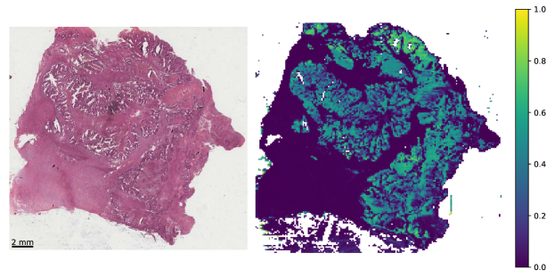
Figure 5: cobra Unsupervised Heatmap. Patient: TCGA-CA-6715

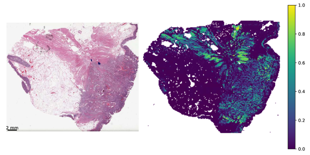
Figure 6: cobra Unsupervised Heatmap. Patient: TCGA-CM-5349

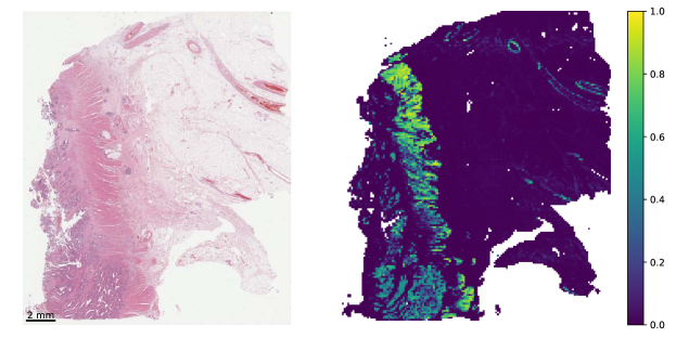
Figure 7: cobra Unsupervised Heatmap. Patient: TCGA-EI-6508

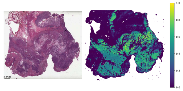
Figure 8: cobra Unsupervised Heatmap. Patient: TCGA-CM-4743

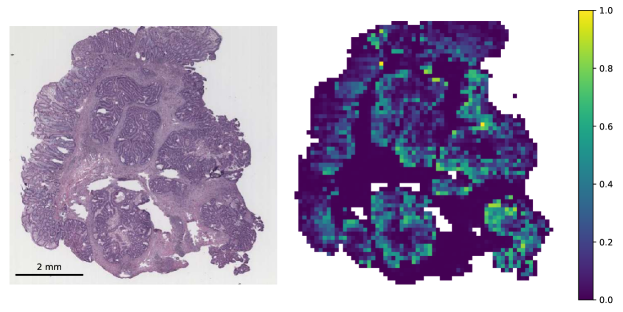
Figure 9: cobra Unsupervised Heatmap. Patient: CPTAC-20CO007

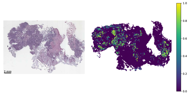
Figure 10: cobra Unsupervised Heatmap. Patient: CPTAC-11CO062

References

- Ba et al. [2016] Jimmy Lei Ba, Jamie Ryan Kiros, and Geoffrey E. Hinton. Layer normalization, 2016.
- Cerami et al. [2012] Ethan Cerami, Jianjiong Gao, Ugur Dogrusoz, Benjamin E Gross, Serdar O Sumer, Bülent A Aksoy, Anders Jacobsen, Christina J Byrne, Michael L Heuer, Erik Larsson, Yevgeniy Antipin, Boris Reva, Allen P Goldberg, Chris Sander, and Nikolaus Schultz. The cbio cancer genomics portal: an open platform for exploring multidimensional cancer genomics data. Cancer discovery, 2(5):401–404, 2012.
- Chen et al. [2022] Richard J. Chen, Chengkuan Chen, Yicong Li, Tiffany Y. Chen, Andrew D. Trister, Rahul G. Krishnan, and Faisal Mahmood. Scaling vision transformers to gigapixel images via hierarchical self-supervised learning. In 2022 IEEE/CVF Conference on Computer Vision and Pattern Recognition (CVPR), pages 16123–16134, 2022.
- Chen et al. [2024] Richard J Chen, Tong Ding, Ming Y Lu, Drew FK Williamson, Guillaume Jaume, Bowen Chen, Andrew Zhang, Daniel Shao, Andrew H Song, Muhammad Shaban, et al. Towards a general-purpose foundation model for computational pathology. Nature Medicine, 2024.
- Chen* et al. [2021] Xinlei Chen*, Saining Xie*, and Kaiming He. An empirical study of training self-supervised vision transformers. arXiv preprint arXiv:2104.02057, 2021.
- Dao and Gu [2024] Tri Dao and Albert Gu. Transformers are ssms: Generalized models and efficient algorithms through structured state space duality, 2024.
- Dietterich et al. [1997] Thomas G. Dietterich, Richard H. Lathrop, and Tomás Lozano-Pérez. Solving the multiple instance problem with axis-parallel rectangles. Artificial Intelligence, 89(1):31–71, 1997.
- Edwards et al. [2015] NJ Edwards, M Oberti, RR Thangudu, S Cai, PB McGarvey, S Jacob, S Madhavan, and KA Ketchum. The cptac data portal: A resource for cancer proteomics research. Journal of Proteome Research, 14(6):2707–2713, 2015. Epub 2015 May 4.
- El Nahhas et al. [2024] Omar S. M. El Nahhas, Marko van Treeck, Georg Wölflein, Michaela Unger, Marta Ligero, Tim Lenz, Sophia J. Wagner, Katherine J. Hewitt, Firas Khader, Sebastian Foersch, Daniel Truhn, and Jakob Nikolas Kather. From whole-slide image to biomarker prediction: end-to-end weakly supervised deep learning in computational pathology. Nature Protocols, 2024.
- Filiot et al. [2023] Alexandre Filiot, Ridouane Ghermi, Antoine Olivier, Paul Jacob, Lucas Fidon, Alice Mac Kain, Charlie Saillard, and Jean-Baptiste Schiratti. Scaling self-supervised learning for histopathology with masked image modeling. medRxiv, 2023.
- Gu and Dao [2024] Albert Gu and Tri Dao. Mamba: Linear-time sequence modeling with selective state spaces, 2024.
- He et al. [2020] Kaiming He, Haoqi Fan, Yuxin Wu, Saining Xie, and Ross Girshick. Momentum contrast for unsupervised visual representation learning. In 2020 IEEE/CVF Conference on Computer Vision and Pattern Recognition (CVPR), pages 9726–9735, 2020.
- Hendrycks and Gimpel [2023] Dan Hendrycks and Kevin Gimpel. Gaussian error linear units (gelus), 2023.
- Huang et al. [2023] Z. Huang, F. Bianchi, M. Yuksekgonul, et al. A visual–language foundation model for pathology image analysis using medical twitter. Nature Medicine, 29:2307–2316, 2023.
- Ilse et al. [2018] Maximilian Ilse, Jakub Tomczak, and Max Welling. Attention-based deep multiple instance learning. In Proceedings of the 35th International Conference on Machine Learning, pages 2127–2136. PMLR, 2018.
- Jaume et al. [2024a] Guillaume Jaume, Lukas Oldenburg, Anurag Vaidya, Richard J. Chen, Drew F. K. Williamson, Thomas Peeters, Andrew H. Song, and Faisal Mahmood. Transcriptomics-guided slide representation learning in computational pathology, 2024a.
- Jaume et al. [2024b] Guillaume Jaume, Anurag Jayant Vaidya, Andrew Zhang, Andrew H Song, Richard J. Chen, Sharifa Sahai, Dandan Mo, Emilio Madrigal, Long Phi Le, and Mahmood Faisal. Multistain pretraining for slide representation learning in pathology. In European Conference on Computer Vision. Springer, 2024b.
- Kang et al. [2023] Mingu Kang, Heon Song, Seonwook Park, Donggeun Yoo, and Sérgio Pereira. Benchmarking self-supervised learning on diverse pathology datasets. In 2023 IEEE/CVF Conference on Computer Vision and Pattern Recognition (CVPR), pages 3344–3354, 2023.
- Koohbanani et al. [2020] Navid Alemi Koohbanani, Balagopal Unnikrishnan, Syed Ali Khurram, Pavitra Krishnaswamy, and Nasir Rajpoot. Self-path: Self-supervision for classification of pathology images with limited annotations, 2020.
- Lazard et al. [2023] Tristan Lazard, Marvin Lerousseau, Etienne Decencière, and Thomas Walter. Giga-ssl: Self-supervised learning for gigapixel images. In 2023 IEEE/CVF Conference on Computer Vision and Pattern Recognition Workshops (CVPRW), pages 4305–4314, 2023.
- Loshchilov and Hutter [2019] Ilya Loshchilov and Frank Hutter. Decoupled weight decay regularization, 2019.
- Lu et al. [2021] Ming Y Lu, Drew FK Williamson, Tiffany Y Chen, Richard J Chen, Matteo Barbieri, and Faisal Mahmood. Data-efficient and weakly supervised computational pathology on whole-slide images. Nature Biomedical Engineering, 5(6):555–570, 2021.
- Lu et al. [2024] Ming-Yu Lu, Bo Chen, Drew F.K. Williamson, et al. A visual-language foundation model for computational pathology. Nature Medicine, 30:863–874, 2024.
- McInnes et al. [2018] Leland McInnes, John Healy, Nathaniel Saul, and Lukas Großberger. Umap: Uniform manifold approximation and projection. Journal of Open Source Software, 3(29):861, 2018.
- Mukashyaka et al. [2024] Patience Mukashyaka, Todd B. Sheridan, Ali Foroughi pour, and Jeffrey H. Chuang. Sampler: unsupervised representations for rapid analysis of whole slide tissue images. eBioMedicine, 99:104908, 2024.
- Nahhas et al. [2024] O. S. M. El Nahhas, C. M. L. Loeffler, Z. I. Carrero, et al. Regression-based deep-learning predicts molecular biomarkers from pathology slides. Nature Communications, 15:1253, 2024.
- Nechaev et al. [2024] Dmitry Nechaev, Alexey Pchelnikov, and Ekaterina Ivanova. Hibou: A family of foundational vision transformers for pathology, 2024.
- Neidlinger et al. [2024] Peter Neidlinger, Omar S. M. El Nahhas, Hannah Sophie Muti, Tim Lenz, Michael Hoffmeister, Hermann Brenner, Marko van Treeck, Rupert Langer, Bastian Dislich, Hans Michael Behrens, Christoph Röcken, Sebastian Foersch, Daniel Truhn, Antonio Marra, Oliver Lester Saldanha, and Jakob Nikolas Kather. Benchmarking foundation models as feature extractors for weakly-supervised computational pathology, 2024.
- Oquab et al. [2024] Maxime Oquab, Timothée Darcet, Théo Moutakanni, Huy Vo, Marc Szafraniec, Vasil Khalidov, Pierre Fernandez, Daniel Haziza, Francisco Massa, Alaaeldin El-Nouby, Mahmoud Assran, Nicolas Ballas, Wojciech Galuba, Russell Howes, Po-Yao Huang, Shang-Wen Li, Ishan Misra, Michael Rabbat, Vasu Sharma, Gabriel Synnaeve, Hu Xu, Hervé Jegou, Julien Mairal, Patrick Labatut, Armand Joulin, and Piotr Bojanowski. Dinov2: Learning robust visual features without supervision, 2024.
- Rong et al. [2014] Weibin Rong, Zhanjing Li, Wei Zhang, and Lining Sun. An improved canny edge detection algorithm. In 2014 IEEE international conference on mechatronics and automation, pages 577–582. IEEE, 2014.
- Saillard et al. [2024] Charlie Saillard, Rodolphe Jenatton, Felipe Llinares-López, Zelda Mariet, David Cahané, Eric Durand, and Jean-Philippe Vert. H-optimus-0, 2024.
- Selvaraju et al. [2019] Ramprasaath R. Selvaraju, Michael Cogswell, Abhishek Das, Ramakrishna Vedantam, Devi Parikh, and Dhruv Batra. Grad-cam: Visual explanations from deep networks via gradient-based localization. International Journal of Computer Vision, 128(2):336–359, 2019.
- Shaikovski et al. [2024] George Shaikovski, Adam Casson, Kristen Severson, Eric Zimmermann, Yi Kan Wang, Jeremy D. Kunz, Juan A. Retamero, Gerard Oakley, David Klimstra, Christopher Kanan, Matthew Hanna, Michal Zelechowski, Julian Viret, Neil Tenenholtz, James Hall, Nicolo Fusi, Razik Yousfi, Peter Hamilton, William A. Moye, Eugene Vorontsov, Siqi Liu, and Thomas J. Fuchs. Prism: A multi-modal generative foundation model for slide-level histopathology, 2024.
- Shao et al. [2021] Zhuchen Shao, Hao Bian, Yang Chen, Yifeng Wang, Jian Zhang, Xiangyang Ji, et al. Transmil: Transformer based correlated multiple instance learning for whole slide image classification. Advances in Neural Information Processing Systems, 34:2136–2147, 2021.
- The Cancer Genome Atlas Research Network et al. [2013] The Cancer Genome Atlas Research Network, J Weinstein, E Collisson, et al. The cancer genome atlas pan-cancer analysis project. Nature Genetics, 45:1113–1120, 2013.
- Unger and Kather [2024] Michaela Unger and Jakob Nikolas Kather. A systematic analysis of deep learning in genomics and histopathology for precision oncology. BMC Medical Genomics, 17(1):48, 2024.
- van den Oord et al. [2019] Aaron van den Oord, Yazhe Li, and Oriol Vinyals. Representation learning with contrastive predictive coding, 2019.
- Vorontsov et al. [2024] E. Vorontsov, A. Bozkurt, A. Casson, et al. A foundation model for clinical-grade computational pathology and rare cancers detection. Nature Medicine, 2024.
- Wagner et al. [2023] SJ Wagner, D Reisenbüchler, NP West, JM Niehues, J Zhu, S Foersch, GP Veldhuizen, P Quirke, HI Grabsch, PA van den Brandt, GGA Hutchins, SD Richman, T Yuan, R Langer, JCA Jenniskens, K Offermans, W Mueller, R Gray, SB Gruber, JK Greenson, G Rennert, JD Bonner, D Schmolze, J Jonnagaddala, NJ Hawkins, RL Ward, D Morton, M Seymour, L Magill, M Nowak, J Hay, VH Koelzer, DN Church, TransSCOT consortium, C Matek, C Geppert, C Peng, C Zhi, X Ouyang, JA James, MB Loughrey, M Salto-Tellez, H Brenner, M Hoffmeister, D Truhn, JA Schnabel, M Boxberg, T Peng, and JN Kather. Transformer-based biomarker prediction from colorectal cancer histology: A large-scale multicentric study. Cancer Cell, 41(9):1650–1661.e4, 2023. Epub 2023 Aug 30.
- Wang et al. [2022] Xiyue Wang, Sen Yang, Jun Zhang, Minghui Wang, Jing Zhang, Wei Yang, Junzhou Huang, and Xiao Han. Transformer-based unsupervised contrastive learning for histopathological image classification. Medical Image Analysis, 2022.
- Wang et al. [2024] X. Wang, J. Zhao, E. Marostica, et al. A pathology foundation model for cancer diagnosis and prognosis prediction. Nature, 2024.
- Wölflein et al. [2024] Georg Wölflein, Dyke Ferber, Asier R. Meneghetti, Omar S. M. El Nahhas, Daniel Truhn, Zunamys I. Carrero, David J. Harrison, Ognjen Arandjelović, and Jakob Nikolas Kather. Benchmarking pathology feature extractors for whole slide image classification, 2024.
- Xu et al. [2024] Hanwen Xu, Naoto Usuyama, Jaspreet Bagga, Sheng Zhang, Rajesh Rao, Tristan Naumann, Cliff Wong, Zelalem Gero, Javier González, Yu Gu, Yanbo Xu, Mu Wei, Wenhui Wang, Shuming Ma, Furu Wei, Jianwei Yang, Chunyuan Li, Jianfeng Gao, Jaylen Rosemon, Tucker Bower, Soohee Lee, Roshanthi Weerasinghe, Bill J. Wright, Ari Robicsek, Brian Piening, Carlo Bifulco, Sheng Wang, and Hoifung Poon. A whole-slide foundation model for digital pathology from real-world data. Nature, 2024.
- Yang et al. [2024] Shu Yang, Yihui Wang, and Hao Chen. MambaMIL: Enhancing Long Sequence Modeling with Sequence Reordering in Computational Pathology . In proceedings of Medical Image Computing and Computer Assisted Intervention – MICCAI 2024. Springer Nature Switzerland, 2024.
- Yu et al. [2023] Zhimiao Yu, Tiancheng Lin, and Yi Xu. Slpd: Slide-level prototypical distillation for wsis, 2023.
- Zimmermann et al. [2024] Eric Zimmermann, Eugene Vorontsov, Julian Viret, Adam Casson, Michal Zelechowski, George Shaikovski, Neil Tenenholtz, James Hall, David Klimstra, Razik Yousfi, Thomas Fuchs, Nicolo Fusi, Siqi Liu, and Kristen Severson. Virchow2: Scaling self-supervised mixed magnification models in pathology, 2024.